Statistical arbitrage under the efficient market hypothesis

Abstract

When a financial derivative can be traded consecutively and its terminal payoffs can be adjusted into a stationary time series, there might be a statistical arbitrage opportunity even under the efficient market hypothesis. In particular, we show the examples of selling put options of the three major ETFs (Exchange Traded Funds) in the U.S. market.

Keywords:

• Stationary process
• statistical arbitrage
• Black–Scholes model

1. Introduction

In economics, an arbitrage is the practice of taking advantage of a price difference between two or more markets: striking a combination of matching deals that capitalise upon the imbalance, the profit being the difference between the market prices. When used by academics, an arbitrage is the possibility of a risk-free profit after transaction costs. For instance, an arbitrage is present when there is the opportunity to instantaneously buy low and sell high.

The celebrated Black–Scholes–Merton's option pricing model (Black & Scholes, 1973; Merton, 1973) is under the efficient market hypothesis, under which there is no arbitrage. This assumption does not conflict with the fact that there are still insurance companies, casino games, etc., which have profits based on the ‘law of large numbers’, which can be considered as the examples of ‘statistical arbitrage’. The term of ‘Statistical Arbitrage’ has been used by various authors with various meanings (see Hogan, Jarrow, & Warachka, 2002; Pole, 2007, for example). In Wang and Zheng (2014), we gave the following general definition. Suppose that $\{X_1,X_2,X_3,\dots \}$ are the gains (may be negative) of a sequence of trades. If $\{X_1,X_2,X_3,\dots \}$ form a stationary sequence with time average asymptotically larger than a positive constant, we call this sequence of trades a ‘statistical arbitrage’. Since we need the realisation of the law of large numbers for the stationary sequence, it is relatively easier to find the examples in high-frequency trading cases, where thousand trades can be made within a not too long period (Wang & Zheng, 2014). Unfortunately, for an individual investor, it is too luxurious to involve in high-frequency trading. In this paper, we show a ‘statistical arbitrage’ opportunity in option trading with rigorous statistical argument, which is a low-frequency (once a week) trading.

In Black–Scholes–Merton's theory, the basic argument is that the seller can match the gap between their option price and the final payoff through hedging. Therefore, their option price is risk-free (also profit-free) to the seller when one ignores all transaction costs and the buyer takes the risk. However, in the real market, a trader has four possible choices of action: selling call option, buying call option, selling put option or buying put option. Therefore, we are wondering if there is some statistical arbitrage opportunity for those practices?

In the basic Black–Scholes's model, the stock price is assumed to be a geometric Brownian motion (Karatzas & Shreve, 1987; Loeve, 1977). That is, $S\left(t\right)=S\left(0\right)\exp \left\{\left(\mu -\frac{{\sigma }^2}{2}\right)t+\sigma W\left(t\right)\right\},$ where $\sigma >0$ is the volatility and μ is a positive constant which should be larger than the interest rate. According to Black–Scholes' formula, one can represent the payoff of a put option with mature time T and strike price K as $(K-S(t){)}^{+}=Q_0+{\int }_0^T{H}_t\mathrm{d}S(t)$ of which the form will not change when μ changes (Cameron–Martin–Girsanov's theorem). Thus if the seller sold this option at $Q_0$ and hedge according to $\left\{H_t\right\},$ he has exactly the money to pay at T. Therefore, one can choose the probability measure which makes the geometric Brownian motion a martingale ($\mu =0$) to get the option price $Q_0$ through taking the mathematical expectation of $(K-S(T){)}^{+}=Q_0+{\int }_0^{T}H(t\left)\mathrm{d}S\right(t).$ Thus the put option price is just the mathematical expectation of $(K-S(T){)}^{+}$ with respect to the risk neutral ($\mu =0$) probability measure. In that formula, the trading volume is 1 share, K and σ are fixed. Our idea is to get a stationary sequence of gains by changing the trading volume and K accordingly to make profit from the positivity of μ by the law of large numbers. More precisely, we may take T = 7 and trade at time $0,T,2T,3T,4T,\dots$ At the closing time of each Friday (time iT), sell put option in $C/S\left(iT\right)$ shares with $K=\kappa S\left(iT\right)$ where κ is fixed.

We actually do not need to assume that the logarithmic price should be a drifted Brownian motion. The only assumption we assumed is that the designed gains form a weakly stationary process with positive mean and asymptotically vanishing covariance, which are statistically tested in the last section.

We separate the remaining part of this paper into three sections: (see Section 2) Examples of statistical arbitrage in option trades; (see Section 3) Mathematical reason and (see Section 4) Statistical tests for our data.

2. Examples of statistical arbitrage in option trades

2.1. Data source and transaction simulation

We consider the option trades of the ETFs (Exchange Traded Funds) of the three major indices in the U.S. market: QQQ (Nasdaq-100 Index ETF), DIA (SPDR Dow Jones Industrial Average ETF) and SPY (SPDR S&P 500 ETF). The daily closing price data of these three major ETFs comes from the Yahoo Finance website. Thus the length of the data varies according to the data obtained. The time range of QQQ data is from 10 March 1999 to 21 February 2017, while DIA ranges from 20 January 1998 to 21 February 2017, and SPY ranges from 29 January 1993 to 21 February 2017. The option data of those three ETFs was bought from the historical option data website.

Since the data of the transaction is at the daily frequency, the slippage of the price has little effect on us. According to our strategy, we can always use the closing price of the week as the trading price to discuss our results, which has little effect to our results. The price spread of the market is ignorable in our cases. In fact, as long as the trading targets are active enough, the price spread is very narrow. In each transaction, we deduct the corresponding transaction fee according to the exchange regulations, which is about a tenth of the total gain in average.

2.2. Methods and results

Suppose that we repeatedly traded the weekly expired options for those three ETFs from the beginning of 2012 in the following way: we sell a volume which is inversely proportional to the current asset price of weekly expired PUT options with strike prices equal to k times the current asset prices. The following three figures show respectively the historical price (Line 1) of QQQ, DIA and SPY, with our accumulated gains for k = 0.99 (Line 2) and k = 1 (Line 3) with volume which is two times of the starting price divided by the current price for those three ETFs. One can do those trades safely as the maintenance requirement for selling those puts are $\frac{1}{6}$ of their current prices (Figures 1–9).

Figure 1. Accumulated gains of selling put options at true-market prices QQQ.

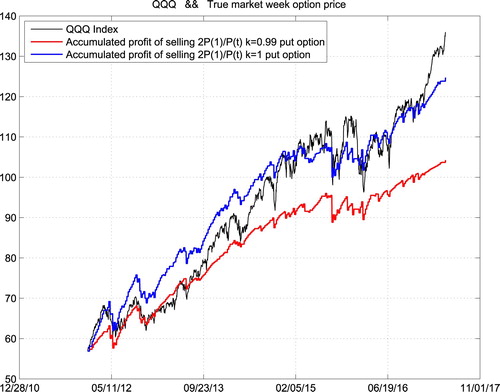
Figure 2. Accumulated gains of selling put options at true-market prices DIA.

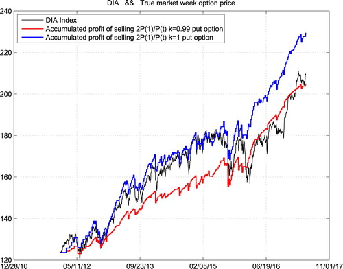
Figure 3. Accumulated gains of selling put options at true-market prices SPY.

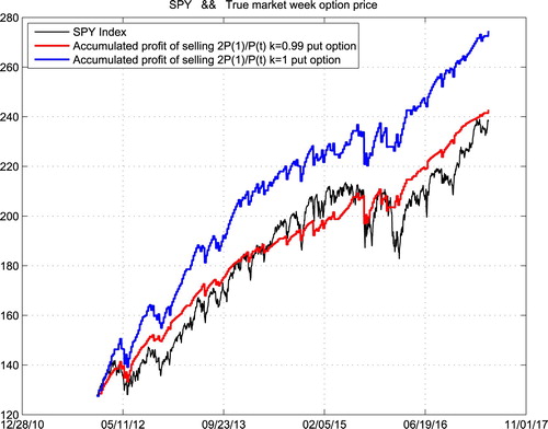
Figure 4. Accumulated gains of selling put options at B-S prices QQQ.

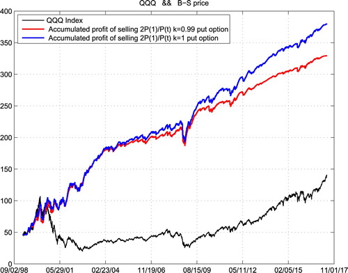
Figure 5. Accumulated gains of selling put options at B-S prices DIA.

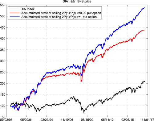
Figure 6. Accumulated gains of selling put options at B-S prices SPY.

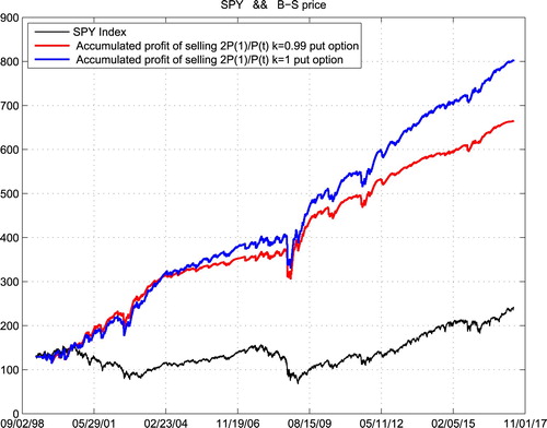
Figure 7. New accumulated gains of selling put options at B-S prices QQQ.

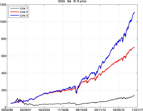
Figure 8. New accumulated gains of selling put options at B-S prices DIA.

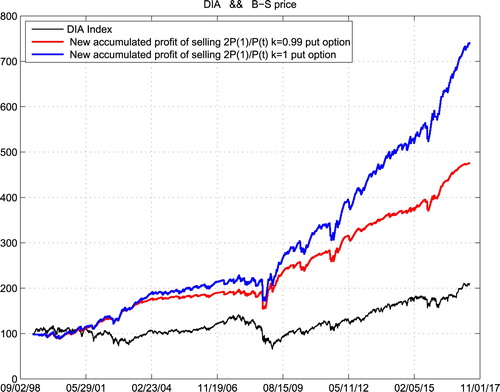
Figure 9. New accumulated gains of selling put options at B-S prices SPY.

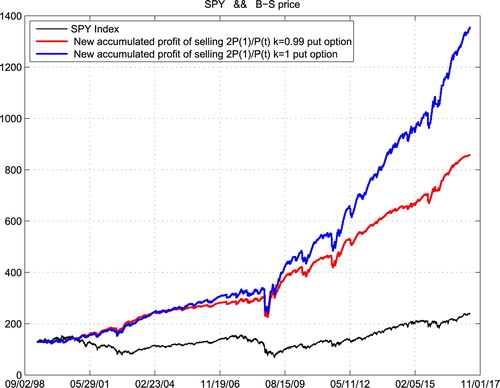
We can easily find that the accumulated profit of our strategy is more stable than operating a roulette machine. Someone may argue that our trading history is not long enough, as the weekly expired options only have 5 years of trading history in the U.S. market which is basically a bull one. Therefore, we show in the following space the accumulated profit of the same strategy for the last 19 years. However, there was no real weekly expired options before 2012. So we use Black–Scholes option prices instead.

In the above six cases, our investment capital was always the starting price $S\left(0\right)$ of the corresponding ETF. We just put aside the accumulated gains. If we reinvest the accumulated gain every 300 trading days as new capital, then we get even better results as the following.

3. Mathematical background of statistical arbitrage

Let us fix a positive integer T. The payoff of $a_i$ shares of European put option with purchasing time iT, mature time $(i+1)T$ and strike price $K_i$ ($i=0,1,2,3,\dots$) is $a_i(K_i-S((i+1)T){)}^{+}.$ The seller's profit at time $(i+1)T$ (without hedging) will be $a_i{Q}_0-a_i(K_i-S((i+1)T){)}^{+}.$ If we can find a sequence of $\left\{\right(K_i,a_i){\}}_i$ such that $\{a_i{Q}_0-a_i(K_i-S\left(\right(i+1\left)T\right){)}^{+}{\}}_i$ form a stationary sequence with a positive mean, then we can get a statistical arbitrage.

In order to get such a stationary sequence, we may choose (at time iT) $K_i=kS\left(iT\right)$ and $a_i=C/S\left(iT\right)$ where C is a fixed amount, k is a prefixed positive percentage constant. Denote $q_i=a_i{Q}_0,$ then the terminal payoff in the time interval $[iT,(i+1\left)T\right]$ will be (1) $C{\left(k-\frac{S\left(\right(i+1\left)T\right)}{S\left(iT\right)}\right)}^{+}$(1) and the seller's profit (without hedging) will be (2) $q_i-C{\left(k-\frac{S\left(\right(i+1\left)T\right)}{S\left(iT\right)}\right)}^{+}$(2) which can also be considered as the corresponding values percentage to the original asset prices. In practice, in order to get profit percentage continuously, we may fix a large constant C and just trade $C/S\left(jT\right)$ shares of options with strike price $kS\left(jT\right)$ (both rounded out to the nearest adequate digits). In Black–Scholes's model, $\{S\left(\right(i+1\left)T\right)/S\left(iT\right){\}}_i$ are just the exponential functions of the increments of Brownian motion, which are independent and identically distributed Gaussian random variables. So the price $q_i$ is the mean of $(S\left(\right(i+1\left)T\right)/S\left(iT\right)-k{)}^{+}$ under the risk-neutral measure, which is a constant. Therefore (1(1) $C{\left(k-\frac{S\left(\right(i+1\left)T\right)}{S\left(iT\right)}\right)}^{+}$(1) ) and (2(2) $q_i-C{\left(k-\frac{S\left(\right(i+1\left)T\right)}{S\left(iT\right)}\right)}^{+}$(2) ) are both independent identically distributed (so they are strongly stationary) in Black–Scholes' theory. If the seller hedges according to Black–Scholes' formula, (2(2) $q_i-C{\left(k-\frac{S\left(\right(i+1\left)T\right)}{S\left(iT\right)}\right)}^{+}$(2) ) is just equal to the hedge result and the seller has neither risk nor profit. Nevertheless, if the seller does not hedge, he will have some small risk like operating a roulette and his profit will be shown in the last three figures of the previous section with large probability.

Since the seller's payoffs (1(1) $C{\left(k-\frac{S\left(\right(i+1\left)T\right)}{S\left(iT\right)}\right)}^{+}$(1) ) are independent identically distributed with mean $Q_{\mu }=E\left[\right(k-\exp \left\{\right(\mu -{\sigma }^2/2)T+\sigma W(T\left)\right\}{)}^{+}]$ depending on μ, we have easily

Theorem 3.1

$Q_{\mu }$ is strictly decreasing in μ.

Proof.

When $\mu >{\mu }^{\prime },$ $\exp \left\{\right(\mu -{\mu }^{\prime }\left)T\right\}>1$. Thus $\begin{array}{rl}& {\left(k-\exp \left\{\left(\mu -\frac{{\sigma }^2}{2}\right)T+\sigma W\left(T\right)\right\}\right)}^{+}\\ & =\left(k-\exp \left\{\right(\mu -{\mu }^{\prime }\left)T\right\}\right.\\ & \times {\left.\exp \left\{\left({\mu }^{\prime }-\frac{{\sigma }^2}{2}\right)T+\sigma W\left(T\right)\right\}\right)}^{+}\\ & \le {\left(k-\exp \left\{\left({\mu }^{\prime }-\frac{{\sigma }^2}{2}\right)T+\sigma W\left(T\right)\right\}\right)}^{+}.\end{array}$ Denote $G(T,\mu )=(k-\exp \{\left(\mu -{\sigma }^2/2\right)T+\sigma W\left(T\right)\}{)}^{+}$, then $\begin{array}{rl}E\left[G\right(T,\mu \left)\right]& ={\int }_{G(T,\mu )>0}G(T,\mu )\\ & <{\int }_{G(T,{\mu }^{\prime })>0}G(T,{\mu }^{\prime })=E\left[G\right(T,\mu \left)\right].\end{array}$ Therefore $\begin{array}{rl}& E\left[{\left(k-\exp \left\{\left(\mu -\frac{{\sigma }^2}{2}\right)T+\sigma W\left(T\right)\right\}\right)}^{+}\right]\\ & <E\left[{\left(k-\exp \left\{\left({\mu }^{\prime }-\frac{{\sigma }^2}{2}\right)T+\sigma W\left(T\right)\right\}\right)}^{+}\right].\end{array}$

In the real market, we always assume that μ is larger than the bond interests. Thus $Q_{\mu }<Q_0$. When we sell the put option at price $Q_0,$ we get the average gain (3) $\begin{array}{rl}& \frac{1}{N}\sum _{i=0}^{N-1}\left\{Q_0-{\left(k-\frac{S\left(\right(i+1\left)T\right)}{S\left(iT\right)}\right)}^{+}\right\}\\ & \to Q_0-Q_{\mu }>0,\end{array}$(3) where the limit holds according to the law of large numbers.

In the real market, we may not have the geometric Brownian motion. However, as long as the sequence of gains is weakly stationary with vanishing covariance, we still may get similar result. We say $\left\{X_t\right\}$ is a ‘weakly stationary’ process, if (i) $E\left[X_t\right]$ is a constant; (ii) $\mathrm{C}\mathrm{o}\mathrm{v}(X_t,X_{t+a})=\mathrm{C}\mathrm{o}\mathrm{v}(X_0,X_a)$ for each t. Certainly, if a strongly stationary process $\left\{X_t\right\}$ has its second moments, then $\left\{X_t\right\}$ is weakly stationary.

Lemma 3.2

Suppose that $\left\{X_j\right\}$ is a weakly stationary sequence such that $\underset{n\to \mathrm{\infty }}{lim}\mathrm{C}\mathrm{o}\mathrm{v}(X_j,X_{j+n})=0,$ then for any $ϵ>0$ $\underset{N\to \mathrm{\infty }}{lim}P\left[\left|\frac{1}{N}\sum _{i=1}^N{X}_{j_i}-E\left[X_1\right]\right|\ge ϵ\right]=0.$

Proof.

$\begin{array}{rl}E{\left|\frac{1}{N}\sum _{i=1}^N{X}_{j_i}-E\left[X_1\right]\right|}^2& \le \frac{1}{N^2}\sum _{i=1}^N\mathrm{V}\mathrm{a}\mathrm{r}\left(X_{j_i}\right)\\ & +\frac{2}{N^2}\sum _{i<k}^N\mathrm{C}\mathrm{o}\mathrm{v}(X_{j_i},X_{j_k}).\end{array}$Thus we get the result by simplification and the classical Chebyshev's inequality.

Therefore, in the next section, we test the weak stationarity and vanishing covariance of gains by statistics.

4. Statistical tests

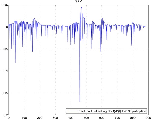
From the previous section and Lemma 3.2, we only need to test two things: (1) stationarity of sequence of gains; (2) covariance tends to 0. Take k = 0.99 for example, Figures 10–12 are the gains of weakly expired options for QQQ, DIA and SPY in the real market, which all pass the test for stationarity. Here, we test the stationarity of the data by the ADF (Augmented Dickey–Fuller) test with Matlab software package and the hypothesis that ‘the sequence has a unit root’ is rejected with 95% of confidence.

Figure 10. Each profit of selling put options at true-market prices QQQ.

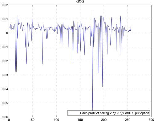
Figure 11. Each profit of selling put options at true-market prices DIA.

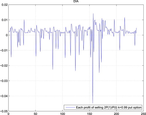
Figure 12. Each profit of selling put options at true-market prices SPY.

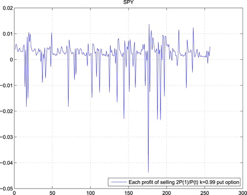
Moreover, Figures 13–15 show the gains of selling put options at Black–Scholes prices, which also pass the test for stationarity.

Figure 13. Each profit of selling put options at B-S prices QQQ.

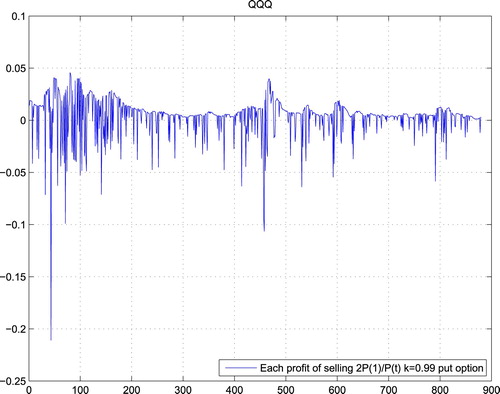
Figure 14. Each profit of selling put options at B-S prices DIA.

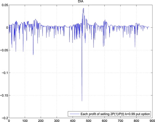
Figure 15. Each profit of selling put options at B-S prices SPY.

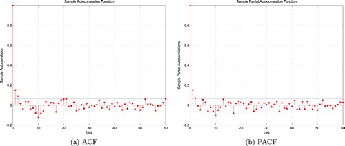
Furthermore, Figures 16–21 plot both the corresponding autocorrelation function (ACF) and sample partial autocorrelation function (PACF) of gains of the above cases. In each graph, the two horizontal lines show the upper and lower bounds of the 95% confidence interval of the corresponding correlation. For any given lag, if the calculated sample autocorrelation or sample partial autocorrelation takes value in this confidence interval, then it is supposed to be 0 under this given lag. Suppose the sample length is N, then, usually, the number of lags takes value of $\sqrt{N}$ or $\log \left(N\right)$, in this case, we take about twice the value. Since most of the sample autocorrelation and sample partial autocorrelation of each case takes value in its 95% confidence interval when lag is larger enough, we accept the hypothesis that the sample autocorrelation tends to 0 when the lag is large enough. That is a common practice in time series analysis (see, e.g., Chapter 4 of Hamilton, 1994).

Figure 16. ACF and PACF of selling QQQ true-market week option: (a) ACF and (b) PACF.

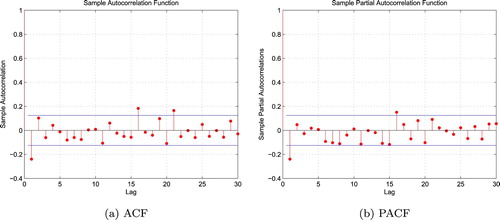
Figure 17. ACF and PACF of selling DIA true-market week option: (a) ACF and (b) PACF.

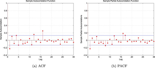
Figure 18. ACF and PACF of selling SPY true-market week option: (a) ACF and (b) PACF.

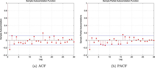
Figure 19. ACF and PACF of selling QQQ B-S week option: (a) ACF and (b) PACF.

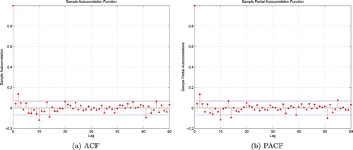
Figure 20. ACF and PACF of selling DIA B-S week option: (a) ACF and (b) PACF.

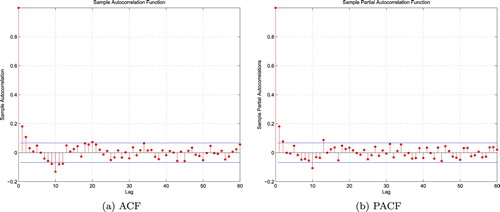
Figure 21. ACF and PACF of selling SPY B-S week option: (a) ACF and (b) PACF.

Disclosure statement

No potential conflict of interest was reported by the authors.

Additional information

Notes on contributors

Si Bao

Si Bao is now working in Xiangcai security Co., LTD. She studied for her Ph.D. in School of Statistics from ECNU.

Shi Chen

Shi Chen is a data scientist of PayPal Holding Inc. He received his Ph.D in statistics from ECNU in 2017.

Xi Wang

Xi Wang is a researcher of DCE Institute for Futures and Options, Beijing. He received his Ph.D in statistics from ECNU in 2018.

Wei An Zheng

Wei An Zheng is Professor of ECNU and Professor Emeritus of University of California, Irvine, USA.

Yu Zhou

Yu Zhou works in Guotai Junan Securities. He received his Ph.D in statistics from ECNU in 2016.

References

- Black, F., & Scholes, M. (1973). The pricing of options and corporate liabilities. Journal of Political Economy, 81(3), 637–654. doi: 10.1086/260062
- Hamilton, J. D. (1994). Time series analysis. Princeton, New Jersey: Princeton University Press.
- Hogan, S., Jarrow, R., & Warachka, M. (2002). Statistical arbitrage and tests of market efficiency. Singapore: Singapore Management University Pre-Prints.
- Karatzas, I., & Shreve, S. E. (1987). Brownian motion and stochastic calculus. Berlin: Springer-Verlag.
- Loeve, M. (1977). Probability theory II. Berlin: Springer-Verlag.
- Merton, R. C. (1973). Theory of rational option pricing. The Bell Journal of Economics and Management Science, 4(1), 141–183. doi: 10.2307/3003143
- Pole, A. (2007). Statistical arbitrage. Inc. Hoboken, New Jersey: John Wiley & Sons.
- Wang, Z. D., & Zheng, W. A. (2014). High frequency trading and probability theory. Singapore: World Scientific.