A resampling approach to estimation of the linking variance in the Fay–Herriot model

ABSTRACT

In the Fay–Herriot model, we consider estimators of the linking variance obtained using different types of resampling schemes. The usefulness of this approach is that even when the estimator from the original data falls below zero or any other specified threshold, several of the resamples can potentially yield values above the threshold. We establish asymptotic consistency of the resampling-based estimator of the linking variance for a wide variety of resampling schemes and show the efficacy of using the proposed approach in numeric examples.

KEYWORDS:

• Linking variance
• Prasad–Rao estimator
• paired bootstrap
• m-out-of-n bootstrap
• Bayesian bootstrap

1. Introduction

A typical survey on any aspect of human behaviour or natural phenomena is limited in scope by feasibility, ethics and cost constraints. Consequently, data are not always obtained in as fine a scale as required by stakeholders. In such cases, small area models are often useful for gathering resources across various domains and variables to obtain estimators and inferences with high precision. Detailed description of small area methods, principles and procedures may be found in the book (Rao & Molina, 2015), and in the papers (Chatterjee, Lahiri, & Li, 2008; Das, Jiang, & Rao, 2004; Datta, Hall, & Mandal, 2011; Datta, Rao, & Smith, 2005; Jiang & Lahiri, 2006; Jiang, Lahiri, & Wan, 2002; Li & Lahiri, 2010; Molina, Rao, & Datta, 2015; Pfeffermann, 2013; Pfeffermann & Glickman, 2004; Rao, 2015; Yoshimori & Lahiri,2014a, 2014b).

In small area studies, arguably the most popular choice of a model for the observed data is the Fay–Herriot model (Fay & Herriot, 1979). This model is described by the following two-layered framework:

1. Sampling model: Conditional on the unknown and unobserved area-level effects $\mathit{\theta }=({\theta }_1,\dots ,{\theta }_n{)}^T$, the sampled and observed data ${\mathbf{Y}}_n=(Y_1,\dots ,Y_n{)}^T$ follows a n-variate Normal distribution with mean $\mathit{\theta }$ and covariance matrix $\mathbf{D}$ with known diagonal entries $D_i>0$ and off-diagonal entries 0. This layer models the sampling level variability and distribution in the observations, conditional on the inherent characteristics $\mathit{\theta }$ of the different small areas.

2. Linking model: The unobserved area-level effects $\mathit{\theta }$ follows a n-variate Normal distribution with mean $X\text{β}$ for a known and non-random $n\times p$ matrix X and unknown but fixed vector $\text{β}\in {\mathbb{R}}^p$. The covariance matrix is $\psi {\mathbb{I}}_n$, where the matrix ${\mathbb{I}}_n$ is the n dimensional identity matrix and $\psi >0$ is an unknown positive-valued constant. This second layer of the Fay–Herriot model links the various small areas together by requiring that all the small areas share a common set of regression parameters $\text{β}\in {\mathbb{R}}^p$ and a common variance component. We assume henceforth that $\psi >\epsilon$ for some small known number ϵ.

Suppose $E\sim N_n(\mathbf{0},\mathbf{D})$ and $U\sim N_n(\mathbf{0},\psi {\mathbb{I}}_n)$ are mutually independent n-dimensional Gaussian random variables, respectively, denoting the errors and random effects. Then we may express the Fay–Herriot model as (1) ${\mathbf{Y}}_n=X\text{β}+U+E\sim N_n(X\text{β},\mathbf{D}+\psi {\mathbb{I}}_n).$(1) In the above Fay–Herriot model, the unknown parameters are the regression parameters $\text{β}\in {\mathbb{R}}^p$ and a common linking variance component $\psi >0$. The distribution of the area-level effects $\mathit{\theta }$, conditional on the data ${\mathbf{Y}}_n$, is the primary quantity of interest in the Fay–Herriot model, and this distribution depends on β and ψ. One traditional approach is to estimate these parameters from data, and then use the estimators in subsequent prediction of $\mathit{\theta }$, conditional on the data ${\mathbf{Y}}_n$.

To assess the quality of prediction in a small area context, we may compute the mean squared prediction error or obtain a prediction interval. The typically Monte Carlo computation-driven technique of resampling is quite popular method for obtaining such intervals and errors bounds and a variety of other purposes, see for example, Chatterjee et al. (2008), Datta et al. (2011), Kubokawa and Nagashima (2012). While most of these papers either use the parametric bootstrap or Efron's original bootstrap (Efron, 1979), other approaches to resampling are also viable, as discussed later in this paper.

One of the intermediate products in all such resampling computations are multiple copies of the estimators of β and ψ obtained from the resamples. The objective of this paper is to assess the quality of such resampling-driven estimators of the original parameters of the data, and we concentrate only on the linking variance parameter ψ here, since it is more critical in subsequent analysis. The immediate purpose of this study is to explore the possibility of using such resampling-based estimators of ψ in case the estimator from the original data takes too low a value.

We present new estimators of ψ, based on the resampling data in a Fay–Herriot model in Section 2, and related theoretical results in Section 3. Some simulation studies are presented in Section 4. Some concluding remarks are included in Section 5.

In the above description of the Fay–Herriot model and in the rest of this paper, we consider all vectors to be column vectors, and for any vector or matrix A, the notation $A^T$ denotes its transpose. For any vector a, the notation $|a|$ stands for its Euclidean norm. The notation $a_i$ will denote the ith element of vector a, similarly $A_{ij}$ will denote the $(i,j)$th element of matrix A. The notation $\mathrm{t}\mathrm{r}\left(A\right)$ denotes the trace of a matrix A, ${\mathcal{I}}_A$ is the indicator function of measurable set A, and $\mathbb{P},\mathbb{E},\mathbb{V}$ are symbols denoting probability, expectation and variance generically. Other notations will be introduced and described as they arise.

We assume that p is fixed and p<n holds, and X is full column rank. We use the notation ${\mathbf{x}}_i$ for the ith row of the matrix X, and ${\mathbf{P}}_{\mathbf{x}}$ for the projection matrix onto the columns of X. In fact, all our results are valid even when p increases with n as long as $p^2/n\to 0$, but the proofs require some additional technicalities. We assume that $n^{-1}{X}^{T}X$ tends towards a positive definite matrix. We also assume that $\underset{1\le i\le n}{max}{\mathbf{P}}_{{\mathbf{x}}_{ii}}=O\left(p/n\right),$ that is, the maximum of the diagonal entries of the projection matrix ${\mathbf{P}}_{\mathbf{x}}$ is of the order of $n^{-1}p$. These conditions are very traditional and standard. We use the notation ${\mathbf{D}}_{\mathbf{x}}$ for the diagonal matrix that has the ith diagonal element as ${\mathbf{P}}_{{\mathbf{x}}_{ii}}$, ie., ${\mathbf{D}}_{\mathbf{x}}$ and ${\mathbf{P}}_{\mathbf{x}}$ share the same diagonal elements but ${\mathbf{D}}_{\mathbf{x}}$ has all off-diagonal elements to be zero. Additionally, we assume that the sampling variances $D_i$'s are bounded above, and away from zero.

2. The resampling-based framework

In the Fay–Herriot model, we implement resampling by associating a non-negative random weight, generically referred to as a resampling weight ${\mathbb{W}}_i$, with the ith observed data point $(Y_i,{\mathbf{x}}_i,D_i)$, for $i=1,\dots ,n$. We assume that these weights are exchangeable and independent of the data, and $\mathbb{E}{\mathbb{W}}_1=\mu >0$ and $\mathbb{V}{\mathbb{W}}_1={\gamma }^2{\mu }^2>0$, where $\gamma >0$. Henceforth we use the notation ${\mathbb{E}}_r$ to denote resampling-expectation, that is, expectation with respect to the distribution of $\mathbb{W}$ conditional on the observed data.

Define $W_i={\gamma }^{-1}{\mu }^{-1}({\mathbb{W}}_i-\mu ),$ for the centred and scaled version of these resampling weights. In minor abuses of notation, we also define $\mathbb{W}$ as a diagonal matrix with the ith diagonal element being ${\mathbb{W}}_i$, and similarly W is a diagonal matrix whose ith diagonal element is $W_i$. Thus we may write $\mathbb{W}=\mu {\mathbb{I}}_n+\gamma \mu W.$

Let $\delta >0$ be a pre-specified constant, and ${\mathcal{A}}_n$ be the set on which the smallest eigenvalue of $X^T\mathbb{W}X$ is higher than δ. Under standard regularity conditions the probability of the set ${\mathcal{A}}_n^C$ is exponentially small, see for example, Chatterjee and Bose (2000). Nevertheless, it is useful to consider the cases ${\mathcal{A}}_n$ and ${\mathcal{A}}_n^C$ separately, since differences arise occasionally with specific choices of $\mathbb{W}$ in numeric computations with finite samples.

Using the resampling weights along with the observed data, the estimator for the regression slope parameters are ${\widehat{\text{β}}}_{nr}=\left\{\begin{array}{ll}(X^T\mathbb{W}X{)}^{-1}{X}^T\mathbb{W}{\mathbf{Y}}_n& \text{on the set }{\mathcal{A}}_n,\\ {\widehat{\text{β}}}_n& \text{otherwise.}\end{array}\right.$ In the above, the second subscript is to denote that this estimator is obtained in the resampling scenario. In the following we describe the case for the set ${\mathcal{A}}_n$ only for brevity, the asymptotically negligible case ${\mathcal{A}}_n^C$ can be addressed using routine algebra. The above leads to the resampling-based fitted values ${\hat{\mathbf{Y}}}_{nr}=X{\widehat{\text{β}}}_{nr}$, and the resulting residuals $\begin{array}{rl}{R}_{nr}& ={\mathbf{Y}}_n-{\hat{\mathbf{Y}}}_{nr}=({\mathbb{I}}_n-X(X^T\mathbb{W}X{)}^{-1}{X}^T\mathbb{W}){\mathbf{Y}}_n\\ & =({\mathbb{I}}_n-X(X^T\mathbb{W}X{)}^{-1}{X}^T\mathbb{W})(E+U).\end{array}$

In the rest of the paper, we study two different resampling-driven estimators of ψ. Let $T_{nr}=\frac{{\mathbb{E}}_r|R_{nr}{|}^2-\mathrm{t}\mathrm{r}({\mathbb{I}}_n+{\gamma }^2{\mathbf{D}}_{\mathbf{x}})({\mathbb{I}}_n-{\mathbf{P}}_{\mathbf{x}})\mathbf{D}({\mathbb{I}}_n-{\mathbf{P}}_{\mathbf{x}})}{\mathrm{t}\mathrm{r}({\mathbb{I}}_n+{\gamma }^2{\mathbf{D}}_{\mathbf{x}})({\mathbb{I}}_n-{\mathbf{P}}_{\mathbf{x}})}$

The resampling-based Prasad–Rao estimator for ψ is defined as (2) ${\hat{\psi }}_{nr}=T_{nr}{\mathcal{I}}_{\{T_{nr}>\epsilon \}}.$(2)

The above estimator is based on Prasad and Rao (1990), where we fit an ordinary least squares regression on the original data ${\mathbf{Y}}_n$ using the covariates X, thus obtaining ${\widehat{\text{β}}}_n=(X^{T}X{)}^{-1}{X}^T{\mathbf{Y}}_n$. Based on the above estimator for β, define the vector of residuals $R=({\mathbb{I}}_n-{\mathbf{P}}_{\mathbf{x}}){\mathbf{Y}}_n$. We use the notation $R_i$ for the ith element of R. The PR estimator for ψis given by (3) ${\hat{\psi }}_n=(n-p{)}^{-1}\left\{|R{|}^2-\sum _{i=1}^n{D}_i+\sum _{i=1}^n({\mathbf{P}}_{\mathbf{x}}\mathbf{D}{)}_i\right\}.$(3)

The second resampling-based estimator of ψ that we study is a variant of the above. Fix a small ${ϵ}_0>0$ that is smaller than the lower bound on ψ. Define the set $\begin{array}{rl}{\mathcal{A}}_{nr}& =\{n^{-1}|R_{nr}{|}^2\ge n^{-1}\mathrm{t}\mathrm{r}({\mathbb{I}}_n+{\gamma }^2{\mathbf{D}}_{\mathbf{x}})({\mathbb{I}}_n-{\mathbf{P}}_{\mathbf{x}})\mathbf{D}\\ & \times ({\mathbb{I}}_n-{\mathbf{P}}_{\mathbf{x}})+{ϵ}_0/2\}.\end{array}$ The alternative resampling-based estimator that we propose is ${\tilde{\psi }}_{nr}=\frac{\begin{array}{c}{\mathbb{E}}_r|R_{nr}{|}^2{\mathcal{I}}_{{\mathcal{A}}_{nr}}-\mathrm{t}\mathrm{r}({\mathbb{I}}_n+{\gamma }^2{\mathbf{D}}_{\mathbf{x}})({\mathbb{I}}_n-{\mathbf{P}}_{\mathbf{x}})\mathbf{D}\\ ({\mathbb{I}}_n-{\mathbf{P}}_{\mathbf{x}})\end{array}}{\mathrm{t}\mathrm{r}({\mathbb{I}}_n+{\gamma }^2{\mathbf{D}}_{\mathbf{x}})({\mathbb{I}}_n-{\mathbf{P}}_{\mathbf{x}})}.$ Note that on the set ${\mathcal{A}}_{nr}$, $|R_{nr}{|}^2$ is greater than $\mathrm{t}\mathrm{r}({\mathbb{I}}_n+{\gamma }^2{\mathbf{D}}_{\mathbf{x}})({\mathbb{I}}_n-{\mathbf{P}}_{\mathbf{x}})\mathbf{D}({\mathbb{I}}_n-{\mathbf{P}}_{\mathbf{x}})$, consequently ${\tilde{\psi }}_{nr}>0$ almost surely. Essentially, the cases where the rth resample has $n^{-1}|R_{nr}{|}^2\le n^{-1}\mathrm{t}\mathrm{r}({\mathbb{I}}_n+{\gamma }^2{\mathbf{D}}_{\mathbf{x}})({\mathbb{I}}_n-{\mathbf{P}}_{\mathbf{x}})\mathbf{D}({\mathbb{I}}_n-{\mathbf{P}}_{\mathbf{x}})+{ϵ}_0/2$ and take an average over the rest of the cases.

This PR estimator is positive almost surely when the intercept is the only covariate but may return a negative value under some circumstances. In fact, an often-encountered challenge in small area studies is to get an estimate of ψ that is positive since standard estimation techniques like the Prasad–Rao method discussed above may result in a potential negative value as an estimate of variance. To address this issue, several techniques have been proposed, see for example Li and Lahiri (2010), Yoshimori and Lahiri (2014a), Hirose and Lahiri (2017), Chatterjee (2018).

Our resampling-based proposed estimators achieve such positive values several times even when ${\hat{\psi }}_n<\epsilon$. We present some numeric examples in Section 4.

Multiple traditional resampling scheme may be realised as special cases of the above framework. Consider a probability experiment where we have n boxes, and n balls, and we allocate balls to boxes randomly and independently, with each ball having the equal probability of 1/n of being allocated to any of the n boxes. The n-dimensional random vector obtained by counting the number of balls in the ith box, for $i=1,\dots ,n$ may be considered as an example of $({\mathbb{W}}_1,\dots ,{\mathbb{W}}_n)$, with $\mu =1$ and $\gamma =(1-n^{-1}{)}^{1/2}$. This example is mathematically identical to the famous paired bootstrap of Efron.

If we modify the above probability experiment slightly, and consider the case where we have only m balls, the above framework obtains $({\mathbb{W}}_1,\dots ,{\mathbb{W}}_n)$ that corresponds to the m-out-of-n bootstrap (referred to as moon-bootstrap in the rest of this paper). If we consider the case where ${\mathbb{W}}_i$ are independent and identically distributed exponential random variables, we obtain variations of the Bayesian bootstrap of Rubin. Other interesting special cases and additional discussion on using resampling weights may be found in Præstgaard and Wellner (1993), Barbe and Bertail (1995), Chatterjee and Bose (2005) and multiple references therein, and in the related chapter of Shao and Tu (1995). The latter classic text, along with the other classic (Efron & Tibshirani, 1993) may be consulted for details about resampling in general.

3. Asymptotic consistency of proposed estimators

We assume that the cross moments on the centred and scaled resampling weights, as in ${\mathbb{E}}_r\prod _{j=1}^J{W}_j^{k_j}$ for small values of J and $\sum _{j=1}^J{k}_j$, do not grow very fast with n. Precise rate at which these grow are available in Chatterjee (1998), Chatterjee and Bose (2000), Chatterjee and Bose (2005) and in other places, and it can be shown easily that such conditions hold for the standard choices of resampling weights. Naturally, when the resampling weights are independent, and the above cross moments are bounded and are often zero, easily satisfy such requirements. We omit detailed discussion on these conditions. We assume that γ is bounded, which is also satisfied by several resampling schemes, but not by others like the moon-bootstrap. Our theoretical results are valid even when we use a controlled rate of growth of γ with n that is applicable to the moon-bootstrap, and our numeric studies validate this later in this paper. However, we discuss only the case of bounded γ to simplify some of the proofs. We now present our main results below.

Theorem 3.1

Under the conditions stated above, the resampling-based Prasad–Rao estimator is asymptotically consistent, that is ${\hat{\psi }}_{nr}\to \psi$ in probability, as $n\to \mathrm{\infty }$.

The different resampling-based estimator ${\tilde{\psi }}_{nr}$, constructed by only considering those resamples where $|R_{nr}{|}^2$ exceeds a threshold, is consistent as well, apart from being always positive. We present this result in the following Theorem:

Theorem 3.2

Under the conditions stated above, ${\tilde{\psi }}_{nr}\to \psi$ in probability, as $n\to \mathrm{\infty }$.

Proof of Theorem 3.1

We omit several algebraic details below, especially those relating to proving asymptotically negligible terms are indeed negligible. Thus, the proof below is a sketch of the main arguments. Below, we use $R_{nk}$ for $k=1,2,3,\dots$ as generic notation for negligible remainder terms. Also, we use c and K, with our without subscripts, as generic notation for constants.

Define $D=\left(X^{T}X{)}^{-1/2}{X}^{T}WX\right(X^{T}X{)}^{-1/2}$. Then $\begin{array}{rl}{X}^T\mathbb{W}X& =\mu (X^{T}X+\gamma X^{T}WX)\\ & =\mu (X^{T}X{)}^{1/2}({\mathbb{I}}_p+\gamma (X^{T}X{)}^{-1/2}{X}^{T}WX\\ & \times \left(X^{T}X{)}^{-1/2})\right(X^{T}X{)}^{1/2}\\ & =\mu (X^{T}X{)}^{1/2}({\mathbb{I}}_p+\gamma D)(X^{T}X{)}^{1/2}.\end{array}$ Thus, $\begin{array}{rl}(X^T\mathbb{W}X{)}^{-1}& ={\mu }^{-1}(X^{T}X{)}^{-1/2}({\mathbb{I}}_p+\gamma D{)}^{-1}\\ & \times (X^{T}X{)}^{-1/2}.\end{array}$ Now notice that $({\mathbb{I}}_p+\gamma D{)}^{-1}={\mathbb{I}}_p-\gamma D+{\gamma }^{2}D({\mathbb{I}}_p+\gamma D{)}^{-1}D.$ Thus $\begin{array}{rl}(X^T\mathbb{W}X{)}^{-1}& ={\mu }^{-1}\left(X^{T}X{)}^{-1/2}({\mathbb{I}}_p+\gamma D{)}^{-1}\right(X^{T}X{)}^{-1/2}\\ & ={\mu }^{-1}(X^{T}X{)}^{-1/2}\{{\mathbb{I}}_p-\gamma D\\ & +{\gamma }^{2}D({\mathbb{I}}_p+\gamma D{)}^{-1}D\}(X^{T}X{)}^{-1/2}\\ & ={\mu }^{-1}[(X^{T}X{)}^{-1}-\gamma (X^{T}X{)}^{-1}{X}^T\\ & \times WX(X^{T}X{)}^{-1}+{\gamma }^2(X^{T}X{)}^{-1}\\ & \left(X^{T}WX\right)(X^{T}X{)}^{-1/2}({\mathbb{I}}_p+\gamma D{)}^{-1}\\ & \times \left(X^{T}X{)}^{-1/2}\right(X^{T}WX\left)\right(X^{T}X{)}^{-1}].\end{array}$ Thus we have $\begin{array}{rl}X(X^T\mathbb{W}X{)}^{-1}{X}^T& ={\mu }^{-1}[{\mathbf{P}}_{\mathbf{x}}-\gamma {\mathbf{P}}_{\mathbf{x}}W{\mathbf{P}}_{\mathbf{x}}+{\gamma }^2{\mathbf{P}}_{\mathbf{x}}\\ & \times WX(X^{T}X{)}^{-1/2}({\mathbb{I}}_p+\gamma D{)}^{-1}\\ & \times (X^{T}X{)}^{-1/2}{X}^{T}W{\mathbf{P}}_{\mathbf{x}}]\\ & ={\mu }^{-1}[{\mathbf{P}}_{\mathbf{x}}-\gamma {\mathbf{P}}_{\mathbf{x}}W{\mathbf{P}}_{\mathbf{x}}+{\gamma }^2{R}_{n1}].\end{array}$

Here, we have $\begin{array}{rl}{R}_{n1}& ={\mathbf{P}}_{\mathbf{x}}WX(X^{T}X{)}^{-1/2}({\mathbb{I}}_p+\gamma D{)}^{-1}\\ & (X^{T}X{)}^{-1/2}{X}^{T}W{\mathbf{P}}_{\mathbf{x}}.\end{array}$ Note that for any non-zero $c\in {\mathbb{R}}^n$ $\begin{array}{rl}{\mathbb{E}}_r\frac{c^T{R}_{n1}c}{c^{T}c}& \le K\frac{c^T{\mathbf{P}}_{\mathbf{x}}{\mathbf{D}}_{\mathbf{x}}{\mathbf{P}}_{\mathbf{x}}c}{c^{T}c}\\ & =O\left(n^{-2}\right).\end{array}$ Thus all eigenvalues of the expectation of $R_{n1}$ are $O\left(n^{-2}\right)$.

This leads us to $\begin{array}{rl}& {\mathbb{I}}_n-X(X^T\mathbb{W}X{)}^{-1}{X}^T\mathbb{W}\\ & ={\mathbb{I}}_n-{\mu }^{-1}[{\mathbf{P}}_{\mathbf{x}}-\gamma {\mathbf{P}}_{\mathbf{x}}W{\mathbf{P}}_{\mathbf{x}}+{\gamma }^2{R}_{n1}]\\ & \times \{\mu ({\mathbb{I}}_n+\gamma W)\}\\ & ={\mathbb{I}}_n-[{\mathbf{P}}_{\mathbf{x}}-\gamma {\mathbf{P}}_{\mathbf{x}}W{\mathbf{P}}_{\mathbf{x}}+{\gamma }^2{R}_{n1}]\{{\mathbb{I}}_n+\gamma W\}\\ & ={\mathbb{I}}_n-{\mathbf{P}}_{\mathbf{x}}+\gamma {\mathbf{P}}_{\mathbf{x}}W{\mathbf{P}}_{\mathbf{x}}-{\gamma }^2{R}_{n1}-\gamma {\mathbf{P}}_{\mathbf{x}}W\\ & +{\gamma }^2{\mathbf{P}}_{\mathbf{x}}W{\mathbf{P}}_{\mathbf{x}}W-{\gamma }^3{R}_{n1}W\\ & =({\mathbb{I}}_n-{\mathbf{P}}_{\mathbf{x}})-\gamma {\mathbf{P}}_{\mathbf{x}}W({\mathbb{I}}_n-{\mathbf{P}}_{\mathbf{x}})\\ & -{\gamma }^2(R_{n1}+\gamma R_{n1}W-{\mathbf{P}}_{\mathbf{x}}W{\mathbf{P}}_{\mathbf{x}}W)\\ & =({\mathbb{I}}_n-\gamma {\mathbf{P}}_{\mathbf{x}}W)({\mathbb{I}}_n-{\mathbf{P}}_{\mathbf{x}})-{\gamma }^2{R}_{n2},\end{array}$ where $R_{n2}=R_{n1}+\gamma R_{n1}W-{\mathbf{P}}_{\mathbf{x}}W{\mathbf{P}}_{\mathbf{x}}W$. We can show that for any non-zero $c\in {\mathbb{R}}^n$ with $|c|=1$, we have $\mathbb{E}{c}^T{R}_{n2}^T{R}_{n2}c=O\left(n^{-4}\right)$. This is algebraic, we omit the details.

So that eventually we get $\begin{array}{rl}{R}_{nr}& =({\mathbb{I}}_n-\gamma {\mathbf{P}}_{\mathbf{x}}W)({\mathbb{I}}_n-{\mathbf{P}}_{\mathbf{x}})(U+E)\\ & -{\gamma }^2{R}_{n2}(U+E).\end{array}$

Hence we can write $\begin{array}{rl}|R_{nr}{|}^2& =\mathrm{t}\mathrm{r}\{({\mathbb{I}}_n-\gamma {\mathbf{P}}_{\mathbf{x}}W{)}^T({\mathbb{I}}_n-\gamma {\mathbf{P}}_{\mathbf{x}}W)\\ & \times ({\mathbb{I}}_n-{\mathbf{P}}_{\mathbf{x}})(U+E)(U+E{)}^T({\mathbb{I}}_n-{\mathbf{P}}_{\mathbf{x}})\}\\ & -2{\gamma }^2(U+E{)}^T{R}_{n2}^T({\mathbb{I}}_n-\gamma {\mathbf{P}}_{\mathbf{x}}W)\\ & \times ({\mathbb{I}}_n-{\mathbf{P}}_{\mathbf{x}})(U+E)+{\gamma }^2(U+E{)}^T\\ & \times R_{n2}^T{R}_{n2}(U+E)\\ & =\mathrm{t}\mathrm{r}\{({\mathbb{I}}_n-\gamma {\mathbf{P}}_{\mathbf{x}}W{)}^T({\mathbb{I}}_n-\gamma {\mathbf{P}}_{\mathbf{x}}W)\\ & \times ({\mathbb{I}}_n-{\mathbf{P}}_{\mathbf{x}})(U+E)(U+E{)}^T({\mathbb{I}}_n-{\mathbf{P}}_{\mathbf{x}})\}\\ & +{\gamma }^2{R}_{n3}\\ & =\mathrm{t}\mathrm{r}[\{{\mathbb{I}}_n-\gamma {\mathbf{P}}_{\mathbf{x}}W-\gamma W{\mathbf{P}}_{\mathbf{x}}+{\gamma }^{2}W{\mathbf{P}}_{\mathbf{x}}W\}\\ & \times \{({\mathbb{I}}_n-{\mathbf{P}}_{\mathbf{x}})(U+E)(U+E{)}^T({\mathbb{I}}_n-{\mathbf{P}}_{\mathbf{x}})\}]\\ & +{\gamma }^2{R}_{n3}.\end{array}$ The exact expression of $R_{n3}$ is available from the above expansion, we do not re-write it to avoid repetitions.

The resampling-expectation of the above is $\begin{array}{rl}{\mathbb{E}}_r|R_{nr}{|}^2& =\mathrm{t}\mathrm{r}{\mathbb{E}}_r[\{{\mathbb{I}}_n-\gamma {\mathbf{P}}_{\mathbf{x}}W-\gamma W{\mathbf{P}}_{\mathbf{x}}+{\gamma }^{2}W{\mathbf{P}}_{\mathbf{x}}W\}\\ & \times \{({\mathbb{I}}_n-{\mathbf{P}}_{\mathbf{x}})(U+E)(U+E{)}^T({\mathbb{I}}_n-{\mathbf{P}}_{\mathbf{x}})\}]\\ & +{\gamma }^2{\mathbb{E}}_r{R}_{n3}\\ & =\mathrm{t}\mathrm{r}[\{{\mathbb{I}}_n+{\gamma }^2{\mathbf{D}}_{\mathbf{x}}\}\{({\mathbb{I}}_n-{\mathbf{P}}_{\mathbf{x}})\\ & \times (U+E)(U+E{)}^T({\mathbb{I}}_n-{\mathbf{P}}_{\mathbf{x}})\}]\\ & +{\gamma }^2{\mathbb{E}}_r{R}_{n3}\\ & =\mathrm{t}\mathrm{r}[\{{\mathbb{I}}_n+{\gamma }^2{\mathbf{D}}_{\mathbf{x}}\}\{({\mathbb{I}}_n-{\mathbf{P}}_{\mathbf{x}})\\ & \times (U+E)(U+E{)}^T({\mathbb{I}}_n-{\mathbf{P}}_{\mathbf{x}})\}]\\ & +{\gamma }^2{\mathbb{E}}_r{R}_{n3}\\ & =\mathrm{t}\mathrm{r}[\{{\mathbb{I}}_n+{\gamma }^2{\mathbf{D}}_{\mathbf{x}}\}({\mathbb{I}}_n-{\mathbf{P}}_{\mathbf{x}})\\ & \times \{\mathbf{D}+\psi {\mathbb{I}}_n+(U{U}^T-\psi {\mathbb{I}}_n)\\ & +(E{E}^T-\mathbf{D})+U{E}^T+E{U}^T\}({\mathbb{I}}_n-{\mathbf{P}}_{\mathbf{x}})]\\ & +{\gamma }^2{\mathbb{E}}_r{R}_{n3}.\end{array}$

Also notice that $\begin{array}{rl}& \mathrm{t}\mathrm{r}({\mathbb{I}}_n+{\gamma }^2{\mathbf{D}}_{\mathbf{x}})({\mathbb{I}}_n-{\mathbf{P}}_{\mathbf{x}})\\ & =\mathrm{t}\mathrm{r}\{{\mathbb{I}}_n-{\mathbf{P}}_{\mathbf{x}}+{\gamma }^2{\mathbf{D}}_{\mathbf{x}}-{\gamma }^2\sum _{i=1}^n{{\mathbf{P}}_{{\mathbf{x}}_{ii}}}^2\}\\ & =O\left(n\right)\end{array}$ with the first term contributing $O\left(n\right)$, the second and third terms contributing $O\left(p\right)=O\left(1\right)$ and the last term contributing $O\left(n^{-1}{p}^2\right)=O\left(n^{-1}\right)$.

We can show, using the computations on $R_{n1}$ and $R_{n2}$ partially presented above, that $\mathbb{E}({\mathbb{E}}_r{R}_{n3}{)}^2=O\left(n\right).$ This computation is algebraic, we present a few instances of the main arguments we use for this step.

Consider the term $T_{n1}=\mathrm{t}\mathrm{r}\{{\mathbb{I}}_n+{\gamma }^2{\mathbf{D}}_{\mathbf{x}}\}({\mathbb{I}}_n-{\mathbf{P}}_{\mathbf{x}})U{E}^T({\mathbb{I}}_n-{\mathbf{P}}_{\mathbf{x}}).$ We have $\begin{array}{rl}{T}_{n1}& =E^T({\mathbb{I}}_n-{\mathbf{P}}_{\mathbf{x}})({\mathbb{I}}_n+{\gamma }^2{\mathbf{D}}_{\mathbf{x}})({\mathbb{I}}_n-{\mathbf{P}}_{\mathbf{x}})U\\ & =\sum _{a,b,c=1}^n\left({\mathbb{I}}_n-{\mathbf{P}}_{\mathbf{x}}{)}_{ab}\right({\mathbb{I}}_n+{\gamma }^2{\mathbf{D}}_{\mathbf{x}}{)}_{bb}({\mathbb{I}}_n-{\mathbf{P}}_{\mathbf{x}}{)}_{bc}{E}_a{U}_c\\ & =\sum _{a,i,c=1}^n({\mathbb{I}}_n-{\mathbf{P}}_{\mathbf{x}}{)}_{ai}(1+{\gamma }^2{\mathbf{P}}_{{\mathbf{x}}_{ii}}\left)\right({\mathbb{I}}_n-{\mathbf{P}}_{\mathbf{x}}{)}_{ic}{E}_a{U}_c.\end{array}$ Thus we have $\begin{array}{rl}\mathbb{E}{T}_{n1}^2& =\mathbb{E}\left\{\sum _{i=1}^n(1+{\gamma }^2{\mathbf{P}}_{{\mathbf{x}}_{ii}})\sum _{a=1}^n({\mathbb{I}}_n-{\mathbf{P}}_{\mathbf{x}}{)}_{ia}{E}_a\right.\\ & \times {\left.\sum _{c=1}^n({\mathbb{I}}_n-{\mathbf{P}}_{\mathbf{x}}{)}_{ic}{U}_c\right\}}^2\\ & =\mathbb{E}\left\{\sum _{i,j=1}^n(1+{\gamma }^2{\mathbf{P}}_{{\mathbf{x}}_{ii}})(1+{\gamma }^2{\mathbf{P}}_{{\mathbf{x}}_{jj}})\right.\\ & \times \sum _{a_1,a_2=1}^n({\mathbb{I}}_n-{\mathbf{P}}_{\mathbf{x}}{)}_{i{a}_1}({\mathbb{I}}_n-{\mathbf{P}}_{\mathbf{x}}{)}_{j{a}_2}{E}_{a_1}{E}_{a_2}\\ & \times \left.\sum _{c_1,c_2=1}^n({\mathbb{I}}_n-{\mathbf{P}}_{\mathbf{x}}{)}_{i{c}_1}({\mathbb{I}}_n-{\mathbf{P}}_{\mathbf{x}}{)}_{i{c}_2}{U}_{c_1}{U}_{c_2}\right\}\\ & =\psi \mathbb{E}\left\{\sum _{i,j=1}^n(1+{\gamma }^2{\mathbf{P}}_{{\mathbf{x}}_{ii}})(1+{\gamma }^2{\mathbf{P}}_{{\mathbf{x}}_{jj}})\right.\\ & \times \sum _{a=1}^n({\mathbb{I}}_n-{\mathbf{P}}_{\mathbf{x}}{)}_{ia}({\mathbb{I}}_n-{\mathbf{P}}_{\mathbf{x}}{)}_{ja}{D}_a\\ & \times \left.\sum _{c=1}^n({\mathbb{I}}_n-{\mathbf{P}}_{\mathbf{x}}{)}_{ic}({\mathbb{I}}_n-{\mathbf{P}}_{\mathbf{x}}{)}_{jc}\right\}.\end{array}$

As an example, consider the second component in the last term above. First, let us deal with the case i=j. Then this term becomes $\begin{array}{rl}\sum _{c=1}^n({\mathbb{I}}_n-{\mathbf{P}}_{\mathbf{x}}{)}_{ic}^2& =(1-{\mathbf{P}}_{{\mathbf{x}}_{ii}}{)}^2+\sum _{c=1}^{n(\ne i)}{{\mathbf{P}}_{\mathbf{x}}}_{ic}^2\\ & =(1-{\mathbf{P}}_{{\mathbf{x}}_{ii}}{)}^2-{\mathbf{P}}_{{\mathbf{x}}_{ii}}+\sum _{c=1}^n{{\mathbf{P}}_{\mathbf{x}}}_{ic}^2\\ & =(1-{\mathbf{P}}_{{\mathbf{x}}_{ii}}{)}^2=O(1).\end{array}$

For the $i\ne j$ case, we have $\begin{array}{rl}\sum _{c=1}^n({\mathbb{I}}_n-{\mathbf{P}}_{\mathbf{x}}{)}_{ic}({\mathbb{I}}_n-{\mathbf{P}}_{\mathbf{x}}{)}_{jc}& =-(1-{\mathbf{P}}_{{\mathbf{x}}_{ii}}){{\mathbf{P}}_{\mathbf{x}}}_{ij}\\ & -(1-{\mathbf{P}}_{{\mathbf{x}}_{jj}}){{\mathbf{P}}_{\mathbf{x}}}_{ij}\\ & +\sum _{c=1}^{n(\ne i,j)}{{\mathbf{P}}_{\mathbf{x}}}_{ic}{{\mathbf{P}}_{\mathbf{x}}}_{jc}\\ & =-{{\mathbf{P}}_{\mathbf{x}}}_{ij}-{{\mathbf{P}}_{\mathbf{x}}}_{ij}\\ & +\sum _{c=1}^n{{\mathbf{P}}_{\mathbf{x}}}_{ic}{{\mathbf{P}}_{\mathbf{x}}}_{jc}\\ & =-{{\mathbf{P}}_{\mathbf{x}}}_{ij}-{{\mathbf{P}}_{\mathbf{x}}}_{ij}+{{\mathbf{P}}_{\mathbf{x}}}_{ij}\\ & =-{\mathbf{P}}_{{\mathbf{x}}_{ij}}\end{array}$ Thus, we essentially repeatedly leverage the properties of a projection matrix for the algebraic computations. We omit further algebraic details, they are typically routine.

If we now write $R_{n4}=\frac{{\mathbb{E}}_r|R_{nr}{|}^2-\mathrm{t}\mathrm{r}({\mathbb{I}}_n+{\gamma }^2{\mathbf{D}}_{\mathbf{x}})({\mathbb{I}}_n-{\mathbf{P}}_{\mathbf{x}})\mathbf{D}}{\mathrm{t}\mathrm{r}({\mathbb{I}}_n+{\gamma }^2{\mathbf{D}}_{\mathbf{x}})({\mathbb{I}}_n-{\mathbf{P}}_{\mathbf{x}})}-\psi ,$ the above computations establish that $\mathbb{E}{R}_{n4}^2\to 0,$ as $n\to \mathrm{\infty }$, thus establishing the result.

Proof of Theorem 3.2

This proof contains several calculations in common with the proof of Theorem 3.1, consequently we only discuss the main ideas, and omit most algebraic details.

Recall from the proof of Theorem 3.1 that $\begin{array}{rl}{n}^{-1}|R_{nr}{|}^2& =n^{-1}\mathrm{t}\mathrm{r}[\{{\mathbb{I}}_n+{\gamma }^2{\mathbf{D}}_{\mathbf{x}}\}({\mathbb{I}}_n-{\mathbf{P}}_{\mathbf{x}})\\ & \times \{\mathbf{D}+\psi {\mathbb{I}}_n+(U{U}^T-\psi {\mathbb{I}}_n)\\ & +(E{E}^T-\mathbf{D})+U{E}^T+E{U}^T\}({\mathbb{I}}_n-{\mathbf{P}}_{\mathbf{x}})]\\ & +n^{-1}{\gamma }^2{\mathbb{E}}_r{R}_{n3}\\ & =X_1+Y_1,\left(\mathrm{s}\mathrm{a}\mathrm{y}\right).\end{array}$

For convenience, let us use the notation $\nu =n^{-1}\mathrm{t}\mathrm{r}({\mathbb{I}}_n+{\gamma }^2{\mathbf{D}}_{\mathbf{x}})({\mathbb{I}}_n-{\mathbf{P}}_{\mathbf{x}})\mathbf{D}({\mathbb{I}}_n-{\mathbf{P}}_{\mathbf{x}})$. We thus have $\begin{array}{rl}\mathbb{P}[{\mathcal{A}}_{nr}^C]& =\mathbb{P}[n^{-1}|R_{nr}{|}^2\le \nu +{ϵ}_0/2]\\ & \le \mathbb{P}[n^{-1}|R_{nr}{|}^2\le \nu +{ϵ}_0/2,|Y_1|>{ϵ}_0/2]\\ & +\mathbb{P}[n^{-1}|R_{nr}{|}^2\le \nu +{ϵ}_0/2,|Y_1|\le {ϵ}_0/2]\\ & \le \mathbb{P}[|Y_1|>{ϵ}_0/2]+\mathbb{P}[X_1\le \nu +{ϵ}_0].\end{array}$

Our previous computations from the proof of Theorem 3.1 now ensure that $\mathbb{E}\left(Y_1^2\right)=O\left(n^{-1}\right)$ as well as $\mathbb{V}\left(X_1\right)=O\left(n^{-1}\right)$, and hence both the above probabilities tend to zero, we omit some of the algebraic details here. Some additional algebraic details are then required to establish that the expectation of the square of the difference between ${\hat{\psi }}_{nr}$ and ${\tilde{\psi }}_{nr}$ is also $O\left(n^{-1}\right)$, thus concluding the proof.

4. Some simulation studies

To understand the finite sample performance of the proposed estimator of ψ, we conducted a simulation study. In this study, we consider a framework based closely on the studies of Datta et al. (2005). We use n=15 observations, and p=3 covariates, one of which is the intercept term, and the other two covariates are random generated in each replication of the experiment and fixed. We fix $\psi =1$ and $\text{β}=(2,3,4{)}^T$. We conduct the experiments with two different choices of the sampling variances. In Experiment 1, we fix the $D_i$'s to be 2.0, 0.6, 0.5, 0.4, 0.2, each repeated 3 times. In Experiment 2, we fix the $D_i$'s to be $20.0,0.6,0.5,0.4,0.2$, each repeated 3 times.

We consider three different resampling schemes in this study. First, we consider $\mathbb{W}$ to be the multinomial random variable corresponding to randomly assigning n balls in n boxes, each with equal probability. This corresponds to the paired bootstrap of Efron. Next, we consider $\mathbb{W}$ to be the multinomial random variable corresponding to randomly assigning $m=\left[n^{0.8}\right]$ balls in n boxes, each with equal probability, which corresponds to the moon-bootstrap. Third, we consider each element of $\mathbb{W}$ to have an exponential distribution with mean 1, thus realising the Bayesian bootstrap. The resampling Monte Carlo size is fixed at 1000 in all cases. The simulation experiment was replicated 200 times, and the results presented below are based on these 200 replications.

First, we enumerate the percentage of times estimators of ψ took values less than $\epsilon ={10}^{-4}$. This number varies on the various parameters used in the simulation experiment, and can approach even $80-90\mathrm{\%}$ when we change only a single $D_i$ value or a parameter value within reasonable range.

In Experiment 1, it can be seen from Table 1 that in approximately $5\mathrm{\%}$ of the simulated datasets, the Prasad–Rao estimator based on the original data obtained a value less than ϵ. In these $6\mathrm{\%}$ of the simulated datasets where the Prasad–Rao estimator took a value less than ϵ, different resampling schemes obtained between 19% and 25% cases where the Prasad–Rao estimator based on the resampling data were above ϵ. In the other $95\mathrm{\%}$ cases where the Prasad–Rao estimator from the original data was greater than ϵ, its resampling data-based versions were typically $93-99\mathrm{\%}$ times greater than ϵ as well. This suggests that using the Prasad–Rao estimator based on the resampling data may significantly improve the numeric performance of estimates of the conditional distribution of $\mathit{\theta }$ given ${\mathbf{Y}}_n$, or related prediction intervals, conditional expectations and so on. In Experiment 2, it can be seen from Table 2 that in approximately $52\mathrm{\%}$ of the simulated datasets, the Prasad–Rao estimator based on the original data obtained a value less than ϵ. Other details are consistent with the findings from Experiment 1.

Table 1. Percentages of cases where different estimators of ψ was below or above $\epsilon ={10}^{-4}$ in Experiment 1.

	Low ${\hat{\psi }}_n$	High ${\hat{\psi }}_n$
Orig.	5.50	94.50
${\hat{\psi }}_{nr}$	High	High
Efron	21.90	97.19
Moon	26.24	93.53
Bayesian	19.83	98.49

Note: The first row denotes the percentages based on the Prasad–Rao estimator applied to the original data, the other rows relate to different resampling techniques used.

Table 2. Percentages of cases where different estimators of ψ was below or above $\epsilon ={10}^{-4}$ in Experiment 2.

	Low ${\hat{\psi }}_n$	High ${\hat{\psi }}_n$
Orig.	52.00	48.00
${\hat{\psi }}_{nr}$	High	High
Efron	6.87	89.46
Moon	11.23	83.70
Bayesian	5.23	93.75

Note: The first row denotes the percentages based on the Prasad–Rao estimator applied to the original data, the other rows relate to different resampling techniques used.

We obtain several plots from Experiment 2. In Figure 1, in the top panel, we present in plot (1) the boxplot of ${\hat{\psi }}_n$ from the 200 replications of the simulation experiment. We also select two such replications at random, one corresponding to a dataset where ${\hat{\psi }}_n\le \epsilon$ and the other where ${\hat{\psi }}_n>\epsilon$. In the top panel of Figure 1, plots (2) and (3) are the resampling estimator ${\hat{\psi }}_{nr}$ obtained using multinomial weights corresponding to the paired bootstrap in the randomly selected dataset for which ${\hat{\psi }}_n\le \epsilon$. Plot (2) is from all resamples, and plot (3) is based on only the resamples where ${\hat{\psi }}_{nr}>\epsilon$. Plots (4) and (5) are ${\hat{\psi }}_{nr}$ obtained using multinomial weights corresponding to the paired bootstrap in the randomly selected dataset for which ${\hat{\psi }}_n>\epsilon$, respectively, based on all resamples and only the resamples where ${\hat{\psi }}_{nr}>\epsilon$. Plot (6) is from the ‘Mix’ estimator proposed by Rubin-Bleuer and You (2016), which is always guaranteed to be positive. While the Mix estimator is always positive, notice that is also seems quite biased.

Figure 1. Boxplots of the Prasad–Rao (PR) estimators from Experiment-2. In the top panel, plot (1) is the boxplot of ${\hat{\psi }}_n$ from the 200 replications of the simulation experiment. The rest of the boxplots are from two randomly selected instances of these replications. Plots (2) and (3) are ${\hat{\psi }}_{nr}$ obtained using multinomial weights corresponding to the paired bootstrap in a case where ${\hat{\psi }}_n\le \epsilon$. Plots (4) and (5) are ${\hat{\psi }}_{nr}$ obtained using multinomial weights corresponding to the paired bootstrap in a case where ${\hat{\psi }}_n>\epsilon$. Plot (6) is the Mix estimator. In the bottom panel, we consider a randomly selected case where ${\hat{\psi }}_n>\epsilon$. The first two boxplots, are from multinomial bootstrap, corresponding respectively to cases where we use all the resamples, and only the ones where ${\hat{\psi }}_{nr}>\epsilon$. The third and fourth are from moon bootstrap and fifth and sixth are from Bayesian bootstrap for all resamples and from resamples with ${\hat{\psi }}_{nr}>\epsilon$, respectively. Plot (7) is the Mix estimator.

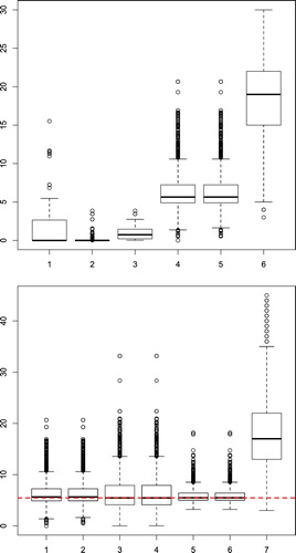
In the bottom panel of Figure 1, we consider a randomly selected case where ${\hat{\psi }}_n>\epsilon$. The first two boxplots are from multinomial bootstrap, corresponding, respectively, to cases where we use all the resamples, and only the ones where ${\hat{\psi }}_{nr}>\epsilon$. The third and fourth are from moon bootstrap and fifth and sixth are from Bayesian bootstrap for all resamples and from resamples with ${\hat{\psi }}_{nr}>\epsilon$, respectively. The last plot is from the Mix estimator, which is again quite biased. The red horizontal line is at the value of ${\hat{\psi }}_n$ for that dataset. It can be seen that all the resampling estimators perform well, especially in cases where ${\hat{\psi }}_n>\epsilon$. For the cases where ${\hat{\psi }}_n\le \epsilon$, the resampling-based estimators offer the alternative of obtaining a higher value of the estimator, while retaining their theoretical consistency properties. Plots from Experiment 1, which we do not present for brevity, are consistent with the above findings.

5. Conclusions

In this paper, we have only studied the resampling-based estimator for the Prasad–Rao formulation: further studies are needed for other choices of estimators. Considerable additional numeric studies are needed. Studies are needed, both from a theoretical as well as computational viewpoint, on the effect of the choice of a resampling-based ψ for prediction of $\mathit{\theta }$. One interesting special case of using resampling weights that needs additional exploration is when γ tends to zero with n, as in the case discussed in Chatterjee and Bose (2002).

Acknowledgments

The author thanks the reviewers and editors for their comments, which helped improve the paper.

Disclosure statement

No potential conflict of interest was reported by the author.

ORCID

Snigdhansu Chatterjee http://orcid.org/0000-0002-7986-0470

Additional information

Funding

This research is partially supported by the National Science Foundation (NSF) [grant numbers # DMS-1622483 and # DMS-1737918].

Notes on contributors

Snigdhansu Chatterjee

Dr. Snigdhansu Chatterjee is Professor in the School of Statistics, and the Director of the Institute for Research in Statistics and its Applications (IRSA, http://irsa.stat.umn.edu/) at the University of Minnesota.

References

- Barbe, P., & Bertail, P (1995). The weighted bootstrap, volume 98 of Lecture Notes in Statistics. New York, NY: Springer-Verlag.
- Chatterjee, S. (1998). Another look at the jackknife: Further examples of generalized bootstrap. Statistics and Probability Letters, 40(4), 307–319.
- Chatterjee, S. (2018). On modifications to linking variance estimators in the Fay-Herriot model that induce robustness. Statistics And Applications, 16(1), 289–303.
- Chatterjee, S., & Bose, A. (2000). Variance estimation in high dimensional regression models. Statistica Sinica, 10(2), 497–516.
- Chatterjee, S., & Bose, A. (2002). Dimension asymptotics for generalised bootstrap in linear regression. Annals of the Institute of Statistical Mathematics, 54(2), 367–381.
- Chatterjee, S., & Bose, A. (2005). Generalized bootstrap for estimating equations. The Annals of Statistics, 33(1), 414–436.
- Chatterjee, S., Lahiri, P., & Li, H. (2008). Parametric bootstrap approximation to the distribution of EBLUP and related prediction intervals in linear mixed models. The Annals of Statistics, 36(3), 1221–1245.
- Das, K., Jiang, J., & Rao, J. N. K. (2004). Mean squared error of empirical predictor. The Annals of Statistics, 32(2), 818–840.
- Datta, G. S., Hall, P., & Mandal, A. (2011). Model selection by testing for the presence of small-area effects, and application to area-level data. Journal of the American Statistical Association, 106(493), 362–374.
- Datta, G. S., Rao, J. N. K., & Smith, D. D. (2005). On measuring the variability of small area estimators under a basic area level model. Biometrika, 92(1), 183–196.
- Efron, B. (1979). Bootstrap methods: Another look at the jackknife. The Annals of Statistics, 7(1), 1–26.
- Efron, B., & Tibshirani, R. J. (1993). An introduction to the bootstrap. Boca Raton, FL: Chapman & Hall/CRC press.
- Fay III, R. E., & Herriot, R. A. (1979). Estimates of income for small places: an application of James-Stein procedures to census data. Journal of the American Statistical Association, 74(366), 269–277.
- Hirose, M. Y., & Lahiri, P (2017). A new model variance estimator for an area level small area model to solve multiple problems simultaneously. arXiv preprint arXiv:1701.04176.
- Jiang, J., & Lahiri, P. (2006). Mixed model prediction and small area estimation (with discussion). Test, 15(1), 1–96.
- Jiang, J., Lahiri, P., & Wan, S.-M. (2002). A unified jackknife theory for empirical best prediction with M-estimation. The Annals of Statistics, 30(6), 1782–1810.
- Kubokawa, T., & Nagashima, B. (2012). Parametric bootstrap methods for bias correction in linear mixed models. Journal of Multivariate Analysis, 106, 1–16.
- Li, H., & Lahiri, P. (2010). An adjusted maximum likelihood method for solving small area estimation problems. Journal of Multivariate Analysis, 101(4), 882–892.
- Molina, I., Rao, J. N. K., & Datta, G. S. (2015). Small area estimation under a Fay–Herriot model with preliminary testing for the presence of random area effects. Survey Methodology, 41(1), 1–19.
- Pfeffermann, D. (2013). New important developments in small area estimation. Statistical Science, 28(1), 40–68.
- Pfeffermann, D., & Glickman, H. (2004). Mean square error approximation in small area estimation by use of parametric and nonparametric bootstrap. ASA Section on Survey Research Methods Proceedings, Alexandria, VA, pp. 4167–4178.
- Prasad, N. G. N., & Rao, J. N. K. (1990). The estimation of the mean squared error of small-area estimators. Journal of the American Statistical Association, 85(409), 163–171.
- Præstgaard, J., & Wellner, J. A. (1993). Exchangeably weighted bootstraps of the general empirical process. The Annals of Probability, 21(4), 2053–2086.
- Rao, J. N. K. (2015). Inferential issues in model-based small area estimation: Some new developments. Statistics in Transition, 16(4), 491–510.
- Rao, J. N. K., & Molina, I. (2015). Small area estimation. New York, NY: Wiley.
- Rubin-Bleuer, S., & You, Y. (2016). Comparison of some positive variance estimators for the Fay–Herriot small area model. Survey Methodology, 42(1), 63–85.
- Shao, J., & Tu, D. (1995). The jackknife and bootstrap. New York, NY: Springer-Verlag.
- Yoshimori, M., & Lahiri, P. (2014a). A new adjusted maximum likelihood method for the Fay–Herriot small area model. Journal of Multivariate Analysis, 124, 281–294.
- Yoshimori, M., & Lahiri, P. (2014b). A second-order efficient empirical Bayes confidence interval. The Annals of Statistics, 42(4), 1233–1261.