Improving timeliness and accuracy of estimates from the UK labour force survey

ABSTRACT

Estimates of unemployment in the UK are based on data collected in the Labour Force Survey (LFS). The data is collected continuously and the survey design is structured in such a way as to provide quarterly estimates. These quarterly estimates are published each month as ‘rolling quarterly’ estimates. Currently the Office for National Statistics (ONS) publish rolling quarterly estimates, and these have been assessed to be of sufficient quality to be badged as ‘National Statistics’. ONS also publish monthly estimates of a selection of labour force variables, but these are designated ‘Experimental Statistics’ due to concerns over the quality of these data. Due to the sample design of the LFS, monthly estimates of change are volatile as there is no sample overlap. A state space model can be used to develop improved estimates of monthly change, accounting for aspects of the survey design. An additional source of information related to unemployment is administrative data on the number of people claiming unemployment related benefits. This data is more timely than survey data collected in the LFS and can be used to provide early estimates of monthly unemployment.

KEYWORDS:

• Unemployment
• rotation group bias
• state space models

1. Introduction

The Office for National Statistics publish monthly statistical bulletins on the UK labour market that include estimates of unemployment (see for example ONS, 2016b). For a statistical bulletin published in month t the latest available estimates of unemployment relate to the quarter covered by months t−4 to t−2, and estimates of changes for these variables look at the change from the quarter covered by months t−7 to t−5. The aim of this paper is to develop methods to improve estimates of monthly change in terms of two important quality measures, accuracy and timeliness.

The current Labour Force Survey (LFS) is designed to provide accurate quarter on quarter estimates of change due to a rotation pattern where given no non-response there is an 80 per cent overlap in respondents. There is user demand for more timely and higher frequency estimates of unemployment and possible options are considered by Steele (1997). As a result of those investigations a decision was made to publish rolling quarterly estimates, as a full redesign of the survey was considered to be too expensive to implement, as described by Werner (2006) who notes that the proposed monthly redesign would have cost an additional seven to eight million pounds. Therefore, while there is a regular monthly publication, the main headline data is essentially quarterly data.

The LFS is a continuous survey as respondents are interviewed each week of the year. Rather than changing the survey design an alternative option for monthly estimates is to account for the rotation pattern of the survey and derive monthly estimates from a state space model. State space models used for estimation in this paper are comprehensively discussed in texts such as Harvey (1990), Durbin and Koopman (2001) and Commandeur and Koopman (2007). Statistics Netherlands and the Bureau of Labor Statistics in the US both use state space models for estimation of some labour force variables such as unemployment (see for example, Tiller, 1992; van den Brakel & Krieg, 2015). Other authors have explored the use of state space models using LFS data from the Australian Bureau of Statistics (ABS), such as Pfeffermann, Feder, and Signorelli (1998), for the Brazilian LFS, Silva and Smith (2001) and also for the UK, such as Harvey and Chung (2000).

Pfeffermann et al. (1998) present a method for estimating the survey error autocorrelation from time series of panel estimates, that for the UK context are called wave-specific estimates. While the correlation of the survey errors could be estimated from the survey data, as is suggested in Tiller (1992) the pseudo-survey error autocorrelation method described by Pfeffermann et al. (1998) does not require this. The benefit of the pseudo-survey error autocorrelation method is the simplicity of the approach as the data required for direct estimation may not be readily available. However, alternative methods could be used, including direct estimation as part of a time series model.

Harvey and Chung (2000) develop bivariate state space models for estimating monthly changes in unemployment for the UK using LFS data and claimant count data (an administrative data source) with a simplified approximation for the correlation deriving it from estimated variances of levels and change. The models presented in Harvey and Chung (2000) demonstrate how using the claimant count, which does not measure the same thing as unemployment, along with survey estimates of unemployment can improve estimates of change due to correlation in the error terms of the modelled population processes.

van den Brakel and Krieg (2009) following the approach by Pfeffermann (1991) take a multivariate approach to develop state space models for monthly unemployment in the Dutch LFS, which has a very similar sample design to that of the UK LFS. Their models are further developed in van den Brakel and Krieg (2016) to include auxiliary administrative data related to unemployment, which as with Harvey and Chung (2000), they find improves the precision of monthly estimates. In the multivariate time series model developed in van den Brakel and Krieg (2009), monthly wave-specific design-based estimates and design-based estimates of variance are used as inputs into the model. The use of the design-based variances are to account for the changing variance over time. This is important in the UK context also, as survey months are either four or five weeks long, and therefore the sample sizes vary by month, and over time there has also been an increase in non-response.

Section 2 provides relevant information on the LFS that inform the structure of the models. Section 3 describes the methods used for estimation of the inputs into the model, and developments of the model from a simpler univariate model to more complex multivariate models that address particular issues in the data from survey error autocorrelation, potential bias, and incorporating administrative data to increase the timeliness as well as the accuracy of unemployment estimates. The models are evaluated in Section 4, while Section 5 concludes.

2. Labour force survey

The Labour Force Survey provides among other things estimates of the number of people in different categories of labour market status (employed, unemployed and inactive) for the target population of people resident in the UK. The LFS has collected data since 1973, although the survey has changed a number of times since then in terms of the data collected and also the frequency at which data is collected. Since 1992 the data collected has been essentially quarterly, although from April 1998 a monthly statistical release has been published which includes rolling-quarterly data for the variables studied here (employment, unemployment and inactivity), which is made possible due to the continuous collection. A history of the LFS can be found in ONS (2016a) and Werner (2006).

This section provides a brief overview of important aspects of the Labour Force Survey (LFS) that are relevant to the development of the time series models developed in later sections, in particular the LFS sample design and estimation methods which are used to create the input data (discussed further in Section 3). As one of the aims of developing models for monthly estimates is to improve their timeliness, the current publication schedule of the main LFS variables are also reviewed.

2.1. Sample design

The LFS is a quarterly survey with a rotating panel design. Respondents in a panel remain in the survey for five successive survey periods, where a survey period is composed of thirteen weeks (labeled ‘stints’, one to thirteen) and respondents asked for their labour market status in the same stint at each survey period. Any quarterly sample period covers the UK population; for samples at frequencies less than quarterly there is a clustering effect due to the survey stints. Assuming full response there should be an eighty per cent overlap in the sample at any thirteen week lag (or one quarter lag) and a twenty per cent overlap in the sample at a four quarter lag. One of the main reasons for this design is to use the sample overlap in order to reduce the variance of estimates of quarterly and annual changes. While in theory it is possible to create weekly or monthly estimates (with a month composed of either four weeks or five weeks and not a strict calendar month), given the smaller sample sizes and also the lack of sample overlap at a weekly or monthly lag, estimates of change at a frequency higher than quarterly are volatile.

As households are in the sample for five successive quarters, each quarter (month or week) it is possible to identify the number of periods the household has already been in the sample for. Grouping the data in this way wave 1 households are those that are selected for the first time, wave 2 households are included for the second time and were initially selected thirteen weeks prior to that date and so on. Therefore households in wave 5 will have been selected at four previous periods at thirteen week intervals. When drawing a sample for any particular quarter, households for waves 2 to 5 will have already been determined by the periods when they were selected to be in wave 1. The wave 1 sample is drawn using a fixed interval of a geographically ordered sampling frame. Further details of the sample design and selection can be found in ONS (2016a).

At wave 1 around 17,380 households are selected for the sample. Therefore, around either five and half or six and half thousand households are selected per survey month (either four or five weeks in length). Response rates in wave 1 tend to be slightly higher at around fifty five per cent and slightly lower for subsequent waves at around forty to forty five per cent (ONS, 2016a, Table 3.3). Responses are requested for all eligible people in the household.

Prior to quarter three 2010, the main LFS was an equal probability sample. However, since then some modifications to the design, such as rolling forward the wave 1 responses of households where all occupants are over the age of seventy five for all subsequent waves and interviewing only one household from addresses with multiple households means that this is no longer the case. Typically responders in wave 1 are interviewed face-to-face with a computer assisted personal interview (CAPI), and in waves 2 to 5 responders are telephoned for a computer assisted telephone interview (CATI).

The important aspects of the sample design and potential for possible forms of bias due to the mode of collection are used for the development of the time series models for survey error and observed systematic differences between wave-specific estimates.

2.2. Estimation methods

Estimates of employment, unemployment and inactivity use calibrated weights that, for the sample, sum to certain known population totals. The calibration groups used for the regular rolling-quarterly data are relatively detailed due to reasonable sample size available for groups. Three calibration groups are used for the LFS including, geographical groups based on Local Authority Districts, an age by sex classification and a cross-classification using sex, age and Government Office Regions. Full details of the calibration groups used can be found in ONS (2016a, Section 10). The calibration helps to deal with potential non-response bias and can also reduce the standard errors of estimators. Population totals are derived from population projections.

Where there is non-response by an individual in a particular wave a response is imputed from their response in the previous wave if a valid response was provided otherwise the case is ignored and weights are appropriately adjusted. This roll-forward imputation only occurs once. If non-response continues no imputation is done and the unit is ignored. Other than the calibration there is no additional non-response weighting in the LFS.

Estimates of accuracy are produced for the main LFS variables using a jacknife linearization method described by Skinner and Holmes (2011) rather than the methods described in ONS (2016a, Annex B). The jackknife estimation method is preferred by Skinner and Holmes (2011) as it may deal more effectively with increases in variance due to varying survey weights.

2.3. Publications

Each month a statistical bulletin on the UK labour market is published which provides estimates of employment, unemployment, inactivity and other employment related statistics, many of which are derived from the LFS, see for example ONS (2016b). The statistical bulletin starts with a section on the main points for the latest three months. The main points usually include the number of people estimated to be in employment and unemployment and how much more or less the latest three month estimate is compared to the three month period from three months previously and also a year ago. The figures presented are seasonally adjusted using the seasonal adjustment software X-13ARIMA-SEATS, Time Series Research Staff (2017). The method of seasonal adjustment used is the X-11 method.

Following the main points section a summary of the latest labour markets statistics is given, which again focuses on current level of variables, rates and also changes on previous periods (essentially quarterly and annual changes). Further on in the bulletin more detailed analysis of the variables is provided, for example, plots of the seasonally adjusted estimates over time with additional commentary.

Towards the end of the bulletin there is a section on accuracy of the estimates, which provides links to data sets on sampling variability with confidence intervals for estimates of levels, rates and changes. It should be noted that the estimates of sampling variability are for the non-seasonally adjusted series rather than the seasonally adjusted estimates that form the main headline figures. Standard errors for seasonally adjusted estimates are not published.

A separate article is published each month for experimental single month LFS estimates, for example see ONS (2017). The article stresses that due to the small sample sizes and no sample overlap the estimates of monthly change are not reliable estimates of current trends in the labour market. The stated main purpose of the single month estimates is to help interpret movements in the headline three-month average rolling quarterly data. As such the single month estimates are benchmarked to the rolling quarterly data and charts included in the article compare the single month with the three-month moving average data.

3. Methods

Estimation of the underlying parameters of interest involves initial estimates of input data for the model followed by the use of a time series model. The input data for the model include design-based monthly wave-specific estimates of unemployment and estimated variances and also estimates of the sample error autocorrelation. Time series models use the wave-specific estimates and their associated variances as input data for the models. The sample error autocorrelation can either be estimated as a hyperparameter in the model, or derived prior to the model using a design-based estimate or the pseudo-survey error autocorrelation approach of Pfeffermann et al. (1998). The models assume that the observed time series are comprised of unobserved components that are estimated with the Kalman filter in the state space framework.

3.1. Input data

Wave-specific time series are estimated using a simplified version of the calibration weighting used for the published rolling-quarterly data. Wave-specific estimates have been estimated from January 2002 onwards, due to the ease of access of the sample data. The wave-specific estimates can be averaged to provide single month time series. It should be noted that the averaged monthly wave-specific estimates differ slightly to the published single month estimates as the method of estimation differs. Information on the current methods for single month estimates can be found in ONS (2017). The sample at any time period less than a quarter is clustered. The variance estimation for the single month wave-specific estimates is done using the linearized jacknife estimator of Skinner and Holmes (2011) accounting for the clustering, stratification and calibration.

Due to the rotation pattern of the LFS, where in theory there should be an eighty per cent overlap in respondents between a survey reference week τ and survey reference week $\tau -13$, there is expected to be a correlation structure to the sampling error. The sampling error autocorrelation of an estimator $y_{\tau }$ from the LFS, is (1) $\begin{array}{r}\mathrm{C}\mathrm{o}\mathrm{r}(y_{\tau },y_{\tau -k})=\left\{\begin{array}{ll}{\rho }_{\tau ,k}& \mathrm{f}\mathrm{o}\mathrm{r}k\in \{0,13,26,39,52\}\\ 0& \mathrm{f}\mathrm{o}\mathrm{r}k\notin \{0,13,26,39,52\}\end{array}\right.\end{array}$(1) Monthly and quarterly estimates are averages of weekly estimates. A quarterly estimate is the average of a thirteen week period, while a monthly estimate is an average of either a four or five week period with three monthly estimates comprising a quarter following a four week plus four week plus five week pattern. If $z_{\tau }$ is an average of weeks $\tau$ to $\tau +l$ then if we assume that the sampling errors follow a stationary process with $\mathrm{V}\mathrm{a}\mathrm{r}\left(y_{\tau }\right)={\sigma }^2$ and $\mathrm{C}\mathrm{o}\mathrm{v}(y_{\tau },y_{\tau -k})={\sigma }_k$ then for monthly or quarterly estimates as $l\le 13$ and only considering lags $k>l$ (that is to say not considering overlapping rolling periods), (2) $\begin{array}{r}\mathrm{C}\mathrm{o}\mathrm{r}(z_{\tau },z_{\tau -k})=\left\{\begin{array}{ll}\frac{{\sigma }_k}{{\sigma }^2}={\rho }_k& \mathrm{f}\mathrm{o}\mathrm{r}k\in \{0,13,26,39,52\}\\ 0& \mathrm{f}\mathrm{o}\mathrm{r}k\notin \{0,13,26,39,52\}\end{array}\right.\end{array}$(2) The expected value of ${\rho }_k$ given no non-response and where there is no change in employment status for those respondents responding at τ and $\tau -k$ is given by the proportion of sample overlap at $k$; ${\rho }_{13}=0.8$. In practice there is non-response and the methods used for imputation as well as the probability of changing employment status between any two periods will mean that the estimated correlation is unlikely to be the theoretical sample overlap. Nevertheless, we may expect to see higher correlation in variables such as employment and inactivity, compared to unemployment, depending upon the labour market conditions. For example, those defined as unemployed should be actively seeking work, and they may be more likely to change labour market status than those who are employed, or those who are inactive (not actively seeking employment).

Pfeffermann et al. (1998) describe a method of estimating what they term pseudo-survey error autocorrelations. Correlation is calculated not directly from the sample data but from the estimated panel time series, that in this paper are referred to as wave-specific estimates. While we can calculate the pseudo-survey error autocorrelation for the series, ${\hat{\rho }}_k$, at lags $k$ it is also possible to estimate the cross correlation between wave-specific time series. For example, we may expect zero correlation at negative lags between the wave 1 sampling errors and other waves as this is the first time that those panel members are included in the sample. We would expect a correlation between wave 2 and wave 1 sampling errors at lags of three months due to the expected eighty per cent sample overlap, a slightly lower correlation between wave 3 and wave 1 sampling errors at lags of six months due to the expected sixty per cent over lap and so on. These pseudo-cross correlations will be used in the development of the multivariate time series models.

The Pfeffermann et al. (1998) method of estimating the pseudo survey error autocorrelation includes terms to address potential rotation group bias, whereby wave-specific time series may have a bias in the level, which could be due, for example, to the mode of data collection.

3.2. Time series models

Three models are compared; a univariate basic structural model of a single month estimate, accounting for survey error autocorrelation and a changing variance over time, a multivariate model using only wave-specific monthly data from the LFS, and an extension to this multivariate model that incorporates an administrative data source related to unemployment called the claimant count. A brief description of the models is given in this section with details on model specification in state space form provided in Appendix. Common to all of the models explored, it is assumed that the population process, $Y_t$, follows a basic structural model given by 4(4) $Y_t=L_t+S_t+I_t,$(4) , that allows for stochastic trend, stochastic seasonal and noise. Models for the survey errors are developed to account for the changing variance over time and also for the survey error correlation. For all models a generalised representation is given, but Section 4 assesses restrictions on the models, to test whether certain variables are required and whether a more parsimonious model is sufficient.

All models have been fitted using the KFAS package (Helske, 2017) in R (R Core Team, 2016). Non-stationary components have diffuse initialization of the Kalman filter, while the unobserved states for the sampling errors have a non-diffuse initialization with mean zero and variance of one. Hyperparameters for the models are estimated using maximum likelihood with the quasi-Newton method BFGS from the optim function in R. Uncertainty arising from the replacement of the unknown true hyperparameters with estimates from maximum likelihood are not accounted for in the standard errors of the estimated unobserved components.

3.2.1. Univariate model

Monthly wave-specific estimates, $y_t^{\left(i\right)}$, for $i=1,2,\dots ,5$, have independent samples at time $t$ across waves $i$, so can be averaged to give a single month estimate, $y_t$. It is assumed that this is comprised of an unobserved population process, $Y_t$, and an autocorrelated survey error process, $e_t$. The survey error is modelled as an AR([3]) process, which denotes an autoregressive process of order three where the coefficients on lag one and two are equal to 0. Design-based variance estimates, $k_t^2$, are also used as input data for the model to account for changing variance over time, in a similar way to the multivariate model discussed in van den Brakel and Krieg (2009). (3) $y_t=Y_t+e_t,$(3) where the population process follows a basic structural model given by (4) $Y_t=L_t+S_t+I_t,$(4) with the trend component, $L_t$ given by (5) $\begin{array}{rl}{L}_t& =L_{t-1}+R_{t-1}+w_t^{\mathrm{L}},w_t^{\mathrm{L}}\sim N(0,{\sigma }_{\mathrm{L}}^2),\end{array}$(5) (6) $\begin{array}{rl}{R}_t& =R_{t-1}+w_t^{\mathrm{R}},w_t^{\mathrm{R}}\sim N(0,{\sigma }_{\mathrm{R}}^2),\end{array}$(6) the seasonal component by (7) $S_t=\sum _{j=1}^{j=6}{S}_{jt}$(7) where for $i=1,\dots ,5$ $\begin{array}{rl}{S}_{jt}& =S_{j,t-1}\cos {\lambda }_j+S_{j,t-1}^{\ast }\sin {\lambda }_j+w_{jt}^{\mathrm{S}},\\ & w_{jt}^{\mathrm{S}}\sim N(0,{\sigma }_{{\mathrm{S}}_j}^2),\\ S_{jt}^{\ast }& =-S_{j,t-1}\sin {\lambda }_j+S_{j,t-1}^{\ast }\cos {\lambda }_j+w_{jt}^{{\mathrm{S}}^{\ast }},\\ & w_{jt}^{{\mathrm{S}}^{\ast }}\sim N(0,{\sigma }_{{\mathrm{S}}_j}^2),\end{array}$ and for j = 6 $S_{jt}=S_{j,t-1}\cos {\lambda }_j+w_{jt}^{\mathrm{S}},w_{jt}^{\mathrm{S}}\sim N(0,{\sigma }_{{\mathrm{S}}_j}^2),$ with $w_{jt}^{\mathrm{S}}$ and $w_{jt}^{{\mathrm{S}}^{\ast }}$ uncorrelated, and unless otherwise specified ${\sigma }_{{\mathrm{S}}_j}^2={\sigma }_{\mathrm{S}}^2$ for all $j$.

The irregular component is given by (8) $I_t=w_t^{\mathrm{I}},w_t^{\mathrm{I}}\sim N(0,{\sigma }_{\mathrm{I}}^2),$(8) and the survey error, assuming an AR([3]) process as (9) $e_t={\phi }_1{e}_{t-3}+{ϵ}_t,{ϵ}_t\sim N(0,(1-{\phi }^2\left){\sigma }_{ϵ}^2{k}_t^2\right).$(9) For the purpose of estimation in the state space framework a similar approach to that introduced by Pfeffermann (1991) and also described by van den Brakel and Krieg (2009) is used where $e_t=k_t{\tilde{e}}_t$, which leads to (10) ${\tilde{e}}_t={\phi }_1{\tilde{e}}_{t-3}+{ϵ}_t,{ϵ}_t\sim N(0,(1-{\phi }_1^2\left){\sigma }_{ϵ}^2\right)$(10) where an estimate of ${\sigma }_{ϵ}^2$ should be approximately equal to 1.

Alternative models for the error or population processes could also be experimented with. Under the assumption that any rotation group bias is approximately constant across time estimating the correlation with a univariate model should not be a problem as any bias should only effect the average level of the time series estimates. Note that ${\phi }_1$ can either be estimated as part of the model, or be estimated using the pseudo-survey error autocorrelation approach or directly from the survey data.

3.2.2. Multivariate model

The multivariate model using only LFS data assumes that the five wave-specific monthly estimates, $y_t^{\left(i\right)}$ for $i=1,2,\dots ,5$, are comprised of the common stochastic population process, $Y_t$, and wave-specific survey errors, $e_t^{\left(i\right)}$. For this model the wave-specific survey error terms are assumed to be comprised of a rotation group bias term, and sampling error which accounts for correlation in the error terms due to sample overlap. The rotation group bias terms are introduced as the observed wave-specific time series differ in level. Given no compelling evidence that the current level of variables are biased the model for the bias terms assumes that the wave-specific bias terms sum to zero.

Wave-specific design-based variance estimates, $(k_t^{\left(i\right)}{)}^2$ for $i=1,2,\dots ,5$, are also used as input data for the model to account for changing variance over time, as discussed in van den Brakel and Krieg (2009). The multivariate model is (11) $y_t^{\left(i\right)}=Y_t+e_t^{\left(i\right)}$(11) where (12) $\begin{array}{rl}{e}_t^{\left(i\right)}& =b_t^{\left(i\right)}+{\epsilon }_t^{\left(i\right)}\end{array}$(12) (13) $\begin{array}{rl}{b}_t^{\left(1\right)}& =-\sum _{i=2}^5{b}_t^{\left(i\right)}\end{array}$(13) (14) $\begin{array}{rl}{b}_t^{\left(i\right)}& =b_{t-1}^{\left(i\right)}+w_t^{\mathrm{b}\left(i\right)},w_t^{\mathrm{b}\left(i\right)}\sim N(0,{\sigma }_{\mathrm{b}\left(i\right)}^2),\\ & \mathrm{f}\mathrm{o}\mathrm{r}i=2,\dots ,5\end{array}$(14) (15) $\begin{array}{rl}{\epsilon }_t^{\left(i\right)}& ={\phi }_1^{\left(i\right)}{\epsilon }_{t-3}^{(i-1)}+{ϵ}_t^{\left(i\right)},\\ {ϵ}_t^{\left(i\right)}& \sim N(0,(1-{\phi }_i^2\left){\sigma }_{ϵ\left(i\right)}^2\right(k_t^{\left(i\right)}{)}^2).\end{array}$(15) Note that in the models ${\sigma }_{ϵ\left(i\right)}^2$ is estimated and should be approximately equal to 1 and with ${\phi }_1=0$, therefore ${\epsilon }_t^{\left(1\right)}={ϵ}_t^{\left(1\right)}$ and $\mathrm{V}\mathrm{a}\mathrm{r}\left({ϵ}_t^{\left(1\right)}\right)=(k_t^{\left(1\right)}{)}^2$.

The model for the wave-specific error is comprised of a wave specific bias term, $b_t^{\left(i\right)}$, which in this case we have assumed sums to zero over all waves, and a wave-specific sampling error. Part of the reason for this assumption is that this is the implicit assumption in the current method of estimation for rolling-quarterly data as no adjustment is made to data for particular waves and the estimator is not considered to be biased. This differs from the assumption made by van den Brakel and Krieg (2009) where wave one is assumed to have no bias and all subsequent waves have a potential bias due to systematic differences in the levels of wave-specific estimates. Alternative models for bias could be considered as discussed in Elliott, Zong, Greenaway, Lacey, and Dixon (2015), which provides some limited evidence that wave one estimates are not found to be biased for the UK. However, it is not possible to conclude from this that other waves are biased and so it is assumed that the bias sums to zero across all waves. The wave specific sampling error, ${\epsilon }_t^{\left(i\right)}$, follows an AR([3]) process which leads to $\mathrm{V}\mathrm{a}\mathrm{r}\left({ϵ}_t^{\left(i\right)}\right)=(1-({\phi }_1^{\left(i\right)}{)}^2\left)\right(k_t^{\left(i\right)}{)}^2$. For the purpose of estimation in the state space framework accounting for the design-based variances, $(k_t^{\left(i\right)}{)}^2$, the same approach as described by van den Brakel and Krieg (2009) is used where ${\epsilon }_t^{\left(i\right)}=k_t^{\left(i\right)}{\tilde{\epsilon }}_t^{\left(i\right)}$, which leads to (16) $\begin{array}{rl}{\tilde{\epsilon }}_t^{\left(i\right)}& ={\phi }_1^{\left(i\right)}{\tilde{\epsilon }}_{t-3}^{(i-1)}+{ϵ}_t^{\left(i\right)},\\ {ϵ}_t^{\left(i\right)}& \sim N(0,(1-\left({\phi }_1^{\left(i\right)}{)}^2\right){\sigma }_{ϵ\left(i\right)}^2)\end{array}$(16) where again estimates of ${\sigma }_{ϵ\left(i\right)}^2$ should be approximately equal to 1 for all $i$.

3.2.3. Multivariate model with claimant count

The multivariate model can be developed further, by incorporating additional administrative data that relates to the variable of interest, which is a similar extension performed by Harvey and Chung (2000) in developing a bivariate model. For example, claimant count data is a measure of those claiming out of work benefits, and while it is not a measure of unemployment based on ILO definitions there is the potential to gain additional accuracy in monthly changes by benefiting from any correlation in unobserved components as shown by Harvey and Chung (2000) for the case of a bivariate model. The multivariate model presented above can be extended to include observed claimant count data as part of the vector of observations ${\mathbf{y}}_t=(y_t^{\left(1\right)},y_t^{\left(2\right)},\dots ,y_t^{\left(5\right)},x_t)$.

If it is assumed that $x_t$ follows a basic structural model (not the common population process for $y_t^{\left(i\right)}$) then covariance terms for the errors in the trend and seasonal components can be incorporated to capture similar movements in the series. To distinguish between population process parameters for unemployment ($Y_t$) and claimant count, superscript $\mathrm{x}$ is used. Hence, Equation (4(4) $Y_t=L_t+S_t+I_t,$(4) ) for claimant count is given by (17) $x_t=L_t^{\mathrm{x}}+S_t^{\mathrm{x}}+I_t^{\mathrm{x}},{\mathrm{e}}_t^{\mathrm{x}}\sim N(0,{\sigma }_{I^{\mathrm{x}}}^2).$(17) Any relationship between the population process for unemployment and claimant count is based on the covariance in error terms, $\mathrm{C}\mathrm{o}\mathrm{v}(w^{\mathrm{L}},w^{{\mathrm{L}}^{\mathrm{x}}})={\sigma }_{\mathrm{L}{\mathrm{L}}^{\mathrm{x}}}$, $\mathrm{C}\mathrm{o}\mathrm{v}(w^{\mathrm{R}},w^{{\mathrm{R}}^{\mathrm{x}}})={\sigma }_{\mathrm{R}{\mathrm{R}}^{\mathrm{x}}}$, $\mathrm{C}\mathrm{o}\mathrm{v}(w^{\mathrm{I}},w^{{\mathrm{I}}^{\mathrm{x}}})={\sigma }_{\mathrm{I}{\mathrm{I}}^{\mathrm{x}}}$, and $\mathrm{C}\mathrm{o}\mathrm{v}(w^{\mathrm{S}},w^{{\mathrm{S}}^{\mathrm{x}}})={\sigma }_{\mathrm{S}{\mathrm{S}}^{\mathrm{x}}}$,.

4. Results

4.1. Survey error autocorrelation

Figure 1 shows the estimated pseudo-survey error autocorrelations and partial autocorrelations for each variable using UK data. Due to the periods of sample overlap, in the following descriptions a lag of l should be read as a lag of $3l$ months. The estimate of autocorrelation at lag 1 (three months) from the pseudo-survey error autocorrelation approach is 0.46. Similar values are obtained by estimating it as a hyperparameter in a univariate state space model (0.4) and the approximation from quarterly design-based variance estimates (0.42). This approximation from design-based estimates uses the approximation in Harvey and Chung (2000) where ${\hat{\rho }}_k\approx 1-\mathrm{v}\mathrm{a}\mathrm{r}(y_t-y_{t-k})/2\mathrm{v}\mathrm{a}\mathrm{r}\left(y_t\right)$. The patterns in the autocorrelation and partial autocorrelations are typical of an autoregressive process of order 1. It should be noted that estimating φ in the univariate model, or using the approximation from design-based estimates does not account for any rotation group bias. For this reason the multi-variate models use the pseudo-survey error autocorrelation. The alternatives methods in the univariate models are presented only to demonstrate the similarities in the estimates.

Figure 1. Pseudo-survey error autocorrelation and partial autocorrelation for UK unemployment ages 16 and over. Note a lag of one is three months as there is no sample overlap between month, so lag $l$, corresponds to a lag of $3l$ months.

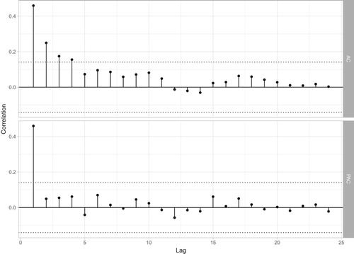
Table 1 shows estimates of wave-specific correlation. There is some evidence of correlation between waves two to five and wave one at the appropriate lag. The correlation between waves is not as high as suggested by sample overlap, which is not surprising as part of the definition of unemployment is actively seeking work. If similar calculations are done for employment or inactivity variables, the correlation tends to be greater. Note when the correlations are calculated on moving windows they are relatively stable over time.

Table 1. Pseudo survey error correlations for unemployment 16 plus by wave. Correlation at lag $l$ for wave $i$ is $\mathrm{C}\mathrm{o}\mathrm{r}({\mathrm{e}}_t^i,{\mathrm{e}}_{t-3l}^{i-l})$.

	Lag 1	Lag 2	Lag 3	Lag 4
Wave 2	0.57	–	–	–
Wave 3	0.54	0.45	–	–
Wave 4	0.52	0.20	0.31	–
Wave 5	0.63	0.32	0.13	0.24

4.2. Univariate models

Table 2 shows estimated hyperparameters for variations on the univariate model, while Table 3 presents standard diagnostics for these models. Other variations on model 1 were also tested but have not been included in the results (these included testing models that included variance parameters ${\sigma }_I^2$ and ${\sigma }_{ϵ}^2$ neither of which gave improvements to the models in Table 3). There is no evidence of lack of normality, heteroscedasticity or autocorrelation in the standardised one-step ahead forecast errors. AIC suggests a model without variance terms for the level or seasonal is preferred. Much of the volatility in the unemployment series is due to the sampling error, and seaosnality is not particularly strong in the series, although it appears to be stable.

Table 2. Estimated hyperparameters for variations on model 1 (univariate) for UK unemployment aged 16 and over.

Variables	Model1a	Model1b	Model1c
${\hat{\sigma }}_L^2$	2.213e−04
${\hat{\sigma }}_R^2$	5.229e−05	6.426e−05	6.426e−05
${\hat{\sigma }}_S^2$	4.208e−37	2.841e−37
φ	4.059e−01	3.716e−01	3.716e−01
AIC	−3.687e+02	−3.703e+02	−3.723e+02

Table 3. Diagnostics based on standardised one-step ahead forecast errors for variations of the univariate model of UK unemployment aged 16 and over including skewness (S), kurtosis (K), Bowman and Shenton test for normality (N), test for Heteroscedasticity (H(h), h indicates sample size), lags that are found to be significant at the 5% level using a Ljung-Box Q(k) test for serial correlation at lag k. See Durbin and Koopman (2001, Section 2.12.1) for test details.

	S	K	N	H(62)	lags Q(k) at 5%
Model 1a	−0.041	3.150	0.227	1.037
Model 1b	−0.053	3.125	0.211	1.002
Model 1c	−0.053	3.125	0.211	1.002

A univariate model was also tested for the claimaint count series to help test subsequent extensions to the multivariate model. The claimant count series follows a similar path to the unemployment data, but is siginficantly less volatile, and seasonality is more evident. Moreover, there is a steeper rise in claimant count than unemployment going into the Great Recession in particular the October 2008 to February 2009 period which causes significant problems for the model in terms of lack of normality, and residual autocorrelation. A sequential step-indicator saturation approach similar to Hendry, Doornik, and Pretis (2013) is used to identify shifts in the level of the series, which can be implemented as j impulse indicator variables ($d_{j,t}$) in the state equation for the trend component such that (18) $L_t^{\mathrm{x}}=L_{t-1}^{\mathrm{x}}+R_{t-1}^{\mathrm{x}}+\sum _j{\text{β}}_j{d}_{j,t-1}+w_t^{{\mathrm{L}}^{\mathrm{x}}}$(18) and coefficients ${\text{β}}_j$ are the magnitude of the level shifts. The variables $d_{j,t}$ are selected by testing the significance of the estimated coefficients by saturating the first half of the sample, followed by the second half of the sample, and then a sequential selection retaining only those variables that are found to be statistically significant at the 0.1% level. This step-indicator saturation approach indientified level shifts at October 2008 (of magnitude 48,234), November 2008 (40,206), January 2009 (104, 929) and February 2009 (31,944). Table 4 shows the improvements in the model diagnostics from including the level shift variables.

Table 4. Diagnostics based on standardised one-step ahead forecast errors for the univariate models of claimaint (without level shift variables, model 1d and with level shift variables, model 1e) including skewness (S), kurtosis (K), Bowman and Shenton test for normality (N), test for Heteroscedasticity (H(h), h indicates sample size), lags that are found to be significant at the 5% level using a Ljung-Box Q(k) test for serial correlation at lag k. See Durbin and Koopman (2001, Section 2.12.1) for test details.

Model	S	K	N	H(79)	lags Q(k) at 5%
Model 1d	0.505	7.487	208.909	1.616	3 to 24
Model 1e	0.022	3.273	0.758	1.286

The seasonality in the claimaint count series is not as stable as that found in the unemployment series. In order to capture the nature of the evolving seasonality sufficiently, frequency-specific seasonal variances are required, as described in Hindrayanto, Aston, Koopman, and Ooms (2013). Based on model selection using AIC, frequency-specific variances include ${\sigma }_{S_1}^2,{\sigma }_{S_2}^2,{\sigma }_{S_{3,4}}^2,{\sigma }_{S_{5,6}}^2$ where $i$ and $j$, in ${\sigma }_{S_{i,j}}^2$ indicate the seasonal frequencies that have been grouped. Further investigations of alternative models for capturing seasonality in the claimant could would be interesting, as it is a stock recorded on the second Thursday of a calendar month, but are not pursued here as the focus is unemployment, and the model for our purposes is sufficient.

4.3. Multivariate models

A similar model selection process to that used for the univariate model was used to identify variance parameters to include in a multivariate model for wave-specific estimates of unemployment, with the wave-specific correlation parameters estimated using the pseudo-survey error autocorrelation approach. The model is then estimated including the claimant count model described in the univariate results section and compared to alternative models that account for possible correlation between the population process for unemployment and claimant count. Three variations of the multivariate model are compared and the hyperparameters and AIC for each are given in Table 5.

Table 5. Estimated hyperparameters for multivariate models: model 2 (independence between unemployment and claimant count), model 3 (covariance terms for both level and slope errors) and model 4 (covariance between slope error terms only) of UK unemployment aged 16 and over and claimant count.

	Model 2	Model 3	Model 4
${\hat{\sigma }}_I^2$		3.079e−08
${\hat{\sigma }}_R^2$	9.024e−05	4.254e−05	4.255e−05
${\hat{\sigma }}_{I^x}^2$	3.995e−06	3.326e−06	3.268e−06
${\hat{\sigma }}_{R^x}^2$	4.034e−05	3.803e−05	3.826e−05
${\hat{\sigma }}_{S_1^x}^2$	5.781e−07	3.136e−06	3.155e−06
${\hat{\sigma }}_{S_2^x}^2$	1.404e−06	1.332e−06	1.333e−06
${\hat{\sigma }}_{S_{3,4}^x}^2$	2.456e−07	2.417e−07	2.417e−07
${\hat{\sigma }}_{S_{5,6}^x}^2$	5.753e−08	5.961e−08	5.930e−08
$\mathrm{C}\mathrm{o}\mathrm{r}(w_t^{\mathrm{I}},w_t^{{\mathrm{I}}^{\mathrm{x}}})$		−1.114e−01
$\mathrm{C}\mathrm{o}\mathrm{r}(w_t^{\mathrm{R}},w_t^{{\mathrm{R}}^{\mathrm{x}}})$		9.707e−01	9.708e−01
AIC	−2.367e+03	−2.407e+03	−2.407e+03

Model 2 treats the multivariate model for unemployemnt and the model for claimant count as independent, whereas model 3 and 4 include covariance terms. Note that in order to test for correlation between the error terms in the irregular component ($\mathrm{C}\mathrm{o}\mathrm{r}(w_t^{\mathrm{I}},w_t^{{\mathrm{I}}^{\mathrm{x}}})$) the population irregular variance for the claimant count (${\hat{\sigma }}_{I^x}^2$) has been moved into the state equation. The addition of covariance terms improves the model, but there is not strong evidence for including covariance terms for both the irregular and the slope. Similarly variance and covariance terms for other components have been tested and are not required. The AIC for model 3 and model 4 are very similar. However, using a likelihood ratio test there is no evidence that inclusion of the additional terms in model 3 is an improvement over model 4, and therefore a covariance term for the slope error terms only is included with an estimated correlation of 0.97.

Table 6 shows diagnostics for the standardised residuals of the multivariate model including claimant count (model 4) which suggests some slight evidence of heteroscedasticity in waves 2 to 3, some evidence of lack of normality for wave 2 and some residual autocorrelation for lags 18 to 24 for wave 1 and lags 21 to 24 in the claimant count. A plot of the cross-correlation of the residuals does not show any strong evidence of correlation at any lags between the different waves and the Doornik-Hansen test for multivariate normality on the standardised residuals from model 4 has a value of 13.61 (p-value of 0.33). Diagnostics for models 2 and 3 are very similar and so are not included here.

Table 6. Diagnostics for model 4 (multivariate) of UK unemployment aged 16 and over including claimant count for skewness (S), kurtosis (K), test for normality (N), test for Heteroscedasticity (H(h)), and lags k for which Ljung-Box Q(k) is significant at the 5% level from the first 24 lags. See Durbin and Koopman (2001, Section 2.12.1) for test details.

Wave	S	K	N	H(62)	lags Q(k) at 5%
1	0.012	3.006	0.005	0.972	18 to 24
2	−0.377	3.609	7.352	1.547
3	−0.271	2.932	2.345	0.645
4	−0.155	3.196	1.058	0.709
5	0.021	2.557	1.550	1.005
Claimant count	0.059	3.053	0.130	1.670	21 to 24

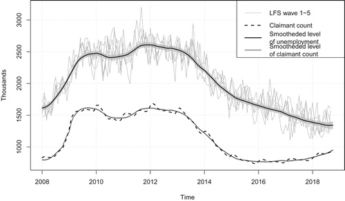
Figure 2 shows the wave-specific estimates for unemployment along with claimant count. The wave-specific estimates are more volatile than published rolling-quarterly data due to the smaller sample sizes. The claimant count is significantly smoother, and the seasonality is more evident. The level of the claimant count is lower than the estimates for unemployment (not all people who are defined as unemployed using the International Labour Organization definition are eligible to claim benefits), but follows similar movements in the trend. Figure 2 also shows the smoothed estimates of the level of unemployment, ${\hat{L}}_{t|T}$ (note that $T=\mathrm{O}\mathrm{c}\mathrm{t}\mathrm{o}\mathrm{b}\mathrm{e}\mathrm{r}2018$, although survey data is only available to September 2018) and claimant count (${\hat{L}}_{t|T}^{\mathrm{x}}$), from multivariate model 4, including claimant count, which as shown by the prediction interval provides a more accurate estimate of the underlying level of unemployment than using wave specific estimates.

Figure 2. LFS wave-specific estimates and smoothed estimate of the level of UK unemployment ages 16 and over from a multivariate model (model 4) including claimant count (grey shaded area is a ninety five percent prediction interval), and level of claimant count.

In a regular publication schedule for monthly data, there is often greater user interest in the latest estimates of change. With smoothed estimates, these will be revised for historical data as new input data become available. Therefore, in order to give an indication of the accuracy of estimates of change from the perspective of a regular monthly publication, the filtered estimates of change are examined. Figure 3 shows the filtered estimate of monthly change in unemployment from the multivariate model 4 which includes claimant count, and shows the gain in accuracy for estimates of change. Using filtered estimates of change in the level of the population process, $R_{t|t}$, much of the time for the period from 2008 onwards monthly change is not significantly different from zero at the five percent level. However, by August 2008 the filtered estimate of the level shows three consecutive periods of monthly increases that are significantly different from zero at the five per cent level. If seasonally adjusted single month estimates were used then there are no periods since 2008 where there are three consecutive monthly increases (or decreases) that are significantly different from zero at the five percent level (using the non-seasonally adjusted standard error as an approximate standard error for the seasonally adjusted series). It is interesting to note that using the rolling-quarterly data three consecutive periods of significant increases are observed a month later in September 2008, suggesting that the modelled single month estimates may be useful for more timely detection of turning points.

Figure 3. Month on month change for LFS single month estimate (seasonally adjusted) and filtered estimate of change of UK unemployment ages 16 and over from a multivariate model including claimant count (grey shaded area is a ninety five percent prediction interval), and monthly change in claimant count (seasonally adjusted).

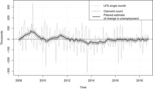
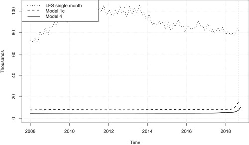
Figure 4 shows the gain in accuracy of the different models compared to the single month estimates. The inclusion of claimant count into the model improves the estimated accuracy of the change in the level component for unemployment. This is due to the correlation in the error terms for the slope components of unemployment and the claimant count. In Figure 4 the multivariate model provides an estimate one month ahead of the univariate model as survey data is not yet available and therefore the estimate from the Kalman filter for the multivariate model borrows some strength from the claimant count which is available one period on from current single month LFS data.

Figure 4. Standard errors of smoothed change in trend from univariate model (model 1c), multivariate model including claimant count (model 4) and original single month, of UK unemployment aged 16 plus.

5. Conclusions

The aim of using time series models is to improve the accuracy and timeliness of single month estimates of unemployment. A simple univariate model that accounts for the survey error autocorrelation structure makes an improvement in accuracy and increases the timeliness compared to the published rolling-quarterly data by one month. Further improvements in accuracy can be gained by using a multivariate model that accounts for both the survey error autocorrelation as well as rotation group bias. An extension to the multivariate model that includes claimant count also improves the accuracy further and also enables an arguably improved one-step ahead forecast of unemployment by drawing on the relationship between unemployment and the claimant count, which would provide an estimate of the level two months ahead of the current rolling-quarter. The gain in accuracy from all models, but particularly the multivariate models, improves the estimates of monthly change which can provide a more timely detection of turning points.

It is interesting to note that there appears to be very little gain in accuracy when extending the univariate model to a multivariate model excluding claimant count, with the larger gains in accuary occuring when claimant count is included. A more parsimonious model, that still benefits from the inclusion of the claimant count might therefore be a bivariate model of unemployment and claimant count as presented in Harvey and Chung (2000). This has not been explored in the current set of models as there is interest from some users and producers of the data in analysing the wave-specific series, and a multivariate model enables a decomposition of this data.

While the inclusion of claimant count appears promising, further research is required on possible discontinuities in the data that have not been picked up in the indicator saturation approach or analysis of the model residuals, as there has been a change to the administration of unemployment related benefits, which might explain the apparent closing of the gap between the average level of unemployment and claimant count.

Common to many of the papers cited throughout this paper, is the assumption that the population process to be measured follows a basic structural model and the sensitivity of this assumption and the implications for estimation of the survey error would be interesting to explore. Some of the papers attempt to deal with changing design-based variance, such as van den Brakel and Krieg (2009), with the assumption that the stochastic nature of the population process itself is not. Depending upon the periods over which the data is analysed, again this may or may not be true and could be difficult to assess what is changes in variance in the survey error and what is changes in variance due to the population process. As noted in the response to Harvey and Chung (2000) by Benoit Quenneville there is the danger than too much of the total variance is assumed to belong to the survey error.

As with many of the papers we find that there is a gain in precision from using the time series model. However, these do not allow for the uncertainty in the maximum likelihood estimates which if accounted for could reduce the impact of such estimated gains. An alternative method that would account for this uncertainty could be to use a Bayesian approach, or a replication technique for estimating the additional uncertainty, as explored for example by Pfeffermann and Tiller (2005).

Acknowledgments

Thanks to two anonymous referees who provided detailed and constructive comments on an earlier submission. Thanks to Danny Pfeffermann for constructive conversations on developing the models. Thanks also to Bethan Russ, Alastair Cameron, Greg Dixon, and Matthew Greenaway for their contributions to providing the wave-specific monthly estimates and variances used as input data for all the modelling.

Disclosure statement

No potential conflict of interest was reported by the authors.

Additional information

Notes on contributors

D. J. Elliott

D. Elliott and P. Zong are methodologists at the Office for National Statistics in the UK.

P. Zong

D. Elliott and P. Zong are methodologists at the Office for National Statistics in the UK.

Appendix. State space models

This appendix provides details of the structure of the univariate and multivariate state space model. State space models enable the estimation of unobserved components of univariate and multivariate time series. The models developed in this paper aim to estimate an underlying stochastic population process and survey error processes, all of which are unobserved. The models used are linear Guassian models.

A.1. State-space framework

The state space framework is comprised of an observation equation and transition equation. The observation equation shows how the unobserved components combine to form the observed values, while the transition equation shows how the unobserved components evolve over time following a first-order Markov process. Following the notation of Harvey (1990) and simplifying slightly to only show aspects that are relevant to the current study the observation and transition equation are respectively (A1) ${\mathbf{y}}_t={\mathbf{Z}}_t{\mathit{\alpha }}_t+{\mathit{ϵ}}_t,$(A1) and (A2) ${\mathit{\alpha }}_t={\mathbf{T}}_t{\mathit{\alpha }}_{t-1}+{\mathbf{R}}_t{\mathit{\eta }}_t,$(A2) where (A3) $\begin{array}{rl}& \mathrm{E}\left({\mathit{ϵ}}_t\right)=0,\mathrm{V}\mathrm{a}\mathrm{r}\left({\mathit{ϵ}}_t\right)={\mathbf{H}}_t,\end{array}$(A3) (A4) $\begin{array}{rl}& \mathrm{E}\left({\mathit{\eta }}_t\right)=0,\mathrm{V}\mathrm{a}\mathrm{r}\left({\mathit{\eta }}_t\right)={\mathbf{Q}}_t.\end{array}$(A4) The observations, ${\mathbf{y}}_t$, may be a multivariate time series with T elements. The state vector of unobserved components is given by ${\mathit{\alpha }}_t$ with dimension $m\times 1$. The observation matrix which combines the unobserved components, ${\mathbf{Z}}_t$ is of dimension $N\times m$ and the observation errors, ${\mathit{ϵ}}_t$, is an $N\times 1$ vector. In the transition equation, ${\mathbf{T}}_t$ is the $m\times m$ transition matrix which defines how that state vector changes over time, ${\mathbf{R}}_t$ is an $m\times q$ matrix determining which elements in the state vector are stochastic, and the transition error, ${\mathit{\eta }}_t$ is an $q\times 1$ vector. ${\mathbf{Z}}_t$, ${\mathbf{T}}_t$, ${\mathbf{R}}_t$, ${\mathbf{H}}_t$ and ${\mathbf{Q}}_t$ are system matrices that are non-stochastic. However they may change over time, hence the time subscript and can contain estimated values, for example the hyperparameters. For details on the estimation of unobserved components using the Kalman filter and methods for hyperparameter estimation see for example Harvey (1990), Durbin and Koopman (2001) or Commandeur and Koopman (2007).

The models in this paper are estimated using the KFAS package of Helske (2017) in the software R, R Core Team (2016). The optimiser used in R from the function optim provides various methods of optimization based on Nelder-Mead, quasi-Newton and conjugate-gradient functions. In this paper BFGS (a quasi-Newton method) is used.

A.2. Univariate model

The basic structural model (Equation (4(4) $Y_t=L_t+S_t+I_t,$(4) )) includes models for the trend (Equation (5(5) $\begin{array}{rl}{L}_t& =L_{t-1}+R_{t-1}+w_t^{\mathrm{L}},w_t^{\mathrm{L}}\sim N(0,{\sigma }_{\mathrm{L}}^2),\end{array}$(5) )) and seasonal component (Equation (7(7) $S_t=\sum _{j=1}^{j=6}{S}_{jt}$(7) )), an irregular component as white noise (Equation (8(8) $I_t=w_t^{\mathrm{I}},w_t^{\mathrm{I}}\sim N(0,{\sigma }_{\mathrm{I}}^2),$(8) )) and sampling error (Equation (9(9) $e_t={\phi }_1{e}_{t-3}+{ϵ}_t,{ϵ}_t\sim N(0,(1-{\phi }^2\left){\sigma }_{ϵ}^2{k}_t^2\right).$(9) )).These equations can be expressed in state space form for monthly data following a similar notation to van den Brakel and Krieg (2009) where ${\mathbf{r}}_{n\times m}$ is a matrix of dimension $n\times m$ where each element is equal to $\mathbf{r}$, ${\mathbf{I}}_n$ is an $n\times n$ identity matrix, $\mathbf{D}\mathbf{i}\mathbf{a}\mathbf{g}$ creates a diagonal matrix from the elements in parentheses, while $\mathbf{B}\mathbf{l}\mathbf{o}\mathbf{c}\mathbf{k}\mathbf{D}\mathbf{i}\mathbf{a}\mathbf{g}$ creates a block diagonal matrix from the elements in parentheses. The model is composed of a population process (θ) and sample error part (e), with the state vector and system matrices given by (A5) $\begin{array}{rl}{\mathit{\alpha }}_t& =({\mathit{\alpha }}_t^{\theta },{\mathit{\alpha }}_t^e{)}^{\mathrm{\prime }},\end{array}$(A5) (A6) $\begin{array}{rl}{\mathbf{Z}}_t& =({\mathbf{Z}}_t^{\theta },{\mathbf{Z}}_t^e),\end{array}$(A6) (A7) $\begin{array}{rl}{\mathbf{T}}_t& =\mathbf{B}\mathbf{l}\mathbf{o}\mathbf{c}\mathbf{k}\mathbf{D}\mathbf{i}\mathbf{a}\mathbf{g}({\mathbf{T}}_t^{\theta },{\mathbf{T}}_t^e),\end{array}$(A7) (A8) $\begin{array}{rl}{\mathbf{R}}_t& =\mathbf{B}\mathbf{l}\mathbf{o}\mathbf{c}\mathbf{k}\mathbf{D}\mathbf{i}\mathbf{a}\mathbf{g}({\mathbf{R}}_t^{\theta },{\mathbf{R}}_t^e),\end{array}$(A8) (A9) $\begin{array}{rl}{\mathbf{H}}_t& ={\sigma }_{ϵ}^2,\end{array}$(A9) (A10) $\begin{array}{rl}{\mathbf{Q}}_t& =\mathbf{D}\mathbf{i}\mathbf{a}\mathbf{g}({\mathbf{Q}}_t^{\theta },{\mathbf{Q}}_t^e),\end{array}$(A10) (A11) $\begin{array}{rl}{\mathit{\alpha }}_t^{\theta }& =(L_t,R_t,S_{1t},S_{1t}^{\ast },\dots ,S_{5t},S_{5t}^{\ast },S_{6t}),\end{array}$(A11) (A12) $\begin{array}{rl}{\mathbf{Z}}_t^{\theta }& =(1,0,1,0,1,0,1,0,1,0,1,0,1),\end{array}$(A12) (A13) $\begin{array}{rl}{\mathbf{T}}_t^{\theta }& =\mathbf{B}\mathbf{l}\mathbf{o}\mathbf{c}\mathbf{k}\mathbf{D}\mathbf{i}\mathbf{a}\mathbf{g}({\mathbf{T}}_t^L,{\mathbf{T}}_t^{S_1},\dots ,{\mathbf{T}}_t^{S_5},\cos {\lambda }_6),\end{array}$(A13) (A14) $\begin{array}{rl}{\mathbf{T}}_t^L& =\left(\begin{array}{cc}1& 1\\ 0& 1\end{array}\right),\end{array}$(A14) (A15) $\begin{array}{rl}{\mathbf{T}}_t^{S_j}& =\left(\begin{array}{cc}\cos {\lambda }_j& \sin {\lambda }_j\\ -\sin {\lambda }_j& \cos {\lambda }_j\end{array}\right),\end{array}$(A15) (A16) $\begin{array}{rl}{\mathbf{R}}_t^{\theta }& ={\mathbf{I}}_{13},\end{array}$(A16) (A17) $\begin{array}{rl}{\mathbf{H}}_t^{\theta }& ={\sigma }_{ϵ}^2,\end{array}$(A17) (A18) $\begin{array}{rl}{\mathbf{Q}}_t^{\theta }& =({\sigma }_L^2,{\sigma }_R^2,{\sigma }_{S_1}^2,{\sigma }_{S_1}^2,{\sigma }_{S_2}^2,{\sigma }_{S_2}^2,{\sigma }_{S_3}^2,{\sigma }_{S_3}^2,{\sigma }_{S_4}^2,{\sigma }_{S_4}^2,\\ & {\sigma }_{S_5}^2,{\sigma }_{S_5}^2,{\sigma }_{S_6}^2).\end{array}$(A18) Design-based variance estimates, $k_t^2$ can be used to account for the changing variance over time as discussed by van den Brakel and Krieg (2009) and used to help obtain estimates of the sampling error. (A19) $\begin{array}{rl}{\mathit{\alpha }}_t^e& =({\tilde{e}}_t,{\tilde{e}}_{t-1},{\tilde{e}}_{t-2}),\end{array}$(A19) (A20) $\begin{array}{rl}{\mathbf{Z}}_t^e& =(k_t,0,0)\end{array}$(A20) (A21) $\begin{array}{rl}{\mathbf{T}}_t^e& =\left(\begin{array}{ccc}0& 0& {\phi }_1\\ 1& 0& 0\\ 0& 1& 0\end{array}\right)\\ {\mathbf{R}}_t^e& =(1,0,0{)}^{\mathrm{\prime }}\end{array}$(A21) (A23) $\begin{array}{rl}{\mathbf{Q}}_t^e& ={\sigma }_{ϵ}^2.\end{array}$(A23)

A.3. Multivariate model

When the observed design-based estimates are monthly wave-specific estimates and assuming the wave-specific survey error and bias terms are combined with the basic structural model and combining with claimant count allowing potentially for correlation, a multivariate state space model can be specified for ${\mathbf{y}}_t=(y_t^{\left(1\right)},y_t^{\left(2\right)},\dots ,y_t^{\left(5\right)},x_t)$ with the state vector and system matrices are given by (A24) $\begin{array}{rl}{\mathit{\alpha }}_t& =({\mathit{\alpha }}_t^{\theta },{\mathit{\alpha }}_t^{\epsilon },{\mathit{\alpha }}_t^b,{\mathit{\alpha }}_t^{{\theta }_x}{)}^{\mathrm{\prime }},\end{array}$(A24) (A25) $\begin{array}{rl}{\mathbf{Z}}_t& =\mathbf{B}\mathbf{l}\mathbf{o}\mathbf{c}\mathbf{k}\mathbf{D}\mathbf{i}\mathbf{a}\mathbf{g}\left(\right(1_{5\times 1}\otimes ({\mathbf{Z}}_t^{\theta }{)}^{\mathrm{\prime }},{\mathbf{Z}}_t^{\epsilon },{\mathbf{Z}}_t^b),{\mathbf{Z}}_t^{\theta }),\end{array}$(A25) (A26) $\begin{array}{rl}{\mathbf{T}}_t& =\mathbf{B}\mathbf{l}\mathbf{o}\mathbf{c}\mathbf{k}\mathbf{D}\mathbf{i}\mathbf{a}\mathbf{g}({\mathbf{T}}_t^{\theta },{\mathbf{T}}_t^{\epsilon },{\mathbf{T}}_t^b,{\mathbf{T}}_t^{\theta }),\end{array}$(A26) (A27) $\begin{array}{rl}{\mathbf{R}}_t& =\mathbf{B}\mathbf{l}\mathbf{o}\mathbf{c}\mathbf{k}\mathbf{D}\mathbf{i}\mathbf{a}\mathbf{g}({\mathbf{R}}_t^{\theta },{\mathbf{R}}_t^{\epsilon },{\mathbf{R}}_t^b,{\mathbf{R}}_t^{\theta }),\end{array}$(A27) (A28) $\begin{array}{rl}{\mathbf{H}}_t& =\mathbf{B}\mathbf{l}\mathbf{o}\mathbf{c}\mathbf{k}\mathbf{D}\mathbf{i}\mathbf{a}\mathbf{g}(0_{5\times 5},{\sigma }_{e_x}^2),\end{array}$(A28) (A29) $\begin{array}{rl}{\mathbf{Q}}_t& =\left(\begin{array}{cc}\mathbf{\text{Diag}}({\mathbf{\text{Q}}}_t^{\theta },{\mathbf{\text{Q}}}_t^{\epsilon },{\mathbf{\text{Q}}}_t^b)& {\mathbf{\text{C}}}^{\mathrm{\prime }}\\ \mathbf{\text{C}}& {\mathbf{\text{Q}}}_t^{{\theta }_x^{\phantom{\int }}}\end{array}\right),\end{array}$(A29) where (A30) $\begin{array}{rl}{\mathit{\alpha }}_t^{\epsilon }& =({\tilde{\epsilon }}_t^{\left(1\right)},{\tilde{\epsilon }}_t^{\left(2\right)},\dots ,{\tilde{\epsilon }}_t^{\left(5\right)},{\tilde{\epsilon }}_{t-1}^{\left(1\right)},{\tilde{\epsilon }}_{t-1}^{\left(2\right)},\dots ,{\tilde{\epsilon }}_{t-1}^{\left(5\right)},\\ & {\tilde{\epsilon }}_{t-2}^{\left(1\right)},{\tilde{\epsilon }}_{t-2}^{\left(2\right)},\dots ,{\tilde{\epsilon }}_{t-2}^{\left(5\right)}),\end{array}$(A30)

(A31) $\begin{array}{rl}{\mathit{\alpha }}_t^b& =(b_t^{\left(2\right)},b_t^{\left(3\right)},b_t^{\left(4\right)},b_t^{\left(5\right)}),\end{array}$(A31) (A32) $\begin{array}{rl}{\mathbf{Z}}_t^{\epsilon }& =\left(\mathbf{D}\mathbf{i}\mathbf{a}\mathbf{g}\right(k_t^{\left(1\right)},k_t^{\left(2\right)},\dots ,k_t^{\left(5\right)}),0_{5\times 10}),\\ {\mathbf{Z}}_t^b& =\left(\begin{array}{cccc}-1& -1& -1& -1\\ 1& 0& 0& 0\\ 0& 1& 0& 0\\ 0& 0& 1& 0\\ 0& 0& 0& 1\end{array}\right),\end{array}$(A32) (A34) $\begin{array}{rl}{\mathbf{T}}_t^{\epsilon }& =\left(\begin{array}{ccccccccccccccc}0& 0& 0& 0& 0& 0& 0& 0& 0& 0& 0& 0& 0& 0& 0\\ 0& 0& 0& 0& 0& 0& 0& 0& 0& 0& {\phi }_1^{\left(2\right)}& 0& 0& 0& 0\\ 0& 0& 0& 0& 0& 0& 0& 0& 0& 0& 0& {\phi }_1^{\left(3\right)}& 0& 0& 0\\ 0& 0& 0& 0& 0& 0& 0& 0& 0& 0& 0& 0& {\phi }_1^{\left(4\right)}& 0& 0\\ 0& 0& 0& 0& 0& 0& 0& 0& 0& 0& 0& 0& 0& {\phi }_1^{\left(5\right)}& 0\\ 1& 0& 0& 0& 0& 0& 0& 0& 0& 0& 0& 0& 0& 0& 0\\ 0& 1& 0& 0& 0& 0& 0& 0& 0& 0& 0& 0& 0& 0& 0\\ 0& 0& 1& 0& 0& 0& 0& 0& 0& 0& 0& 0& 0& 0& 0\\ 0& 0& 0& 1& 0& 0& 0& 0& 0& 0& 0& 0& 0& 0& 0\\ 0& 0& 0& 0& 1& 0& 0& 0& 0& 0& 0& 0& 0& 0& 0\\ 0& 0& 0& 0& 0& 1& 0& 0& 0& 0& 0& 0& 0& 0& 0\\ 0& 0& 0& 0& 0& 0& 1& 0& 0& 0& 0& 0& 0& 0& 0\\ 0& 0& 0& 0& 0& 0& 0& 1& 0& 0& 0& 0& 0& 0& 0\\ 0& 0& 0& 0& 0& 0& 0& 0& 1& 0& 0& 0& 0& 0& 0\\ 0& 0& 0& 0& 0& 0& 0& 0& 0& 1& 0& 0& 0& 0& 0\end{array}\right),\end{array}$(A34) (A35) $\begin{array}{rl}{\mathbf{T}}_t^b& ={\mathbf{I}}_4,\end{array}$(A35) (A36) $\begin{array}{rl}{\mathbf{R}}_t^{\epsilon }& =\left(\begin{array}{c}{\mathbf{I}}_5\\ 0_{10\times 5}\end{array}\right),\end{array}$(A36) (A37) $\begin{array}{rl}{\mathbf{R}}_t^b& ={\mathbf{I}}_4,\\ {\mathbf{Q}}_t^{\epsilon }& =(1,(1-\left({\phi }_1^{\left(2\right)}{)}^2\right),(1-({\phi }_1^{\left(3\right)}{)}^2),(1-\left({\phi }_1^{\left(4\right)}{)}^2\right),\\ & (1-({\phi }_1^{\left(5\right)}{)}^2\left)\right),\end{array}$(A37) (A39) $\begin{array}{rl}{\mathbf{Q}}_t^b& =({\sigma }_{b2}^2,{\sigma }_{b3}^2,{\sigma }_{b4}^2,{\sigma }_{b5}^2).\\ {\mathit{\alpha }}_t^{{\theta }_x}& =(L_t^x,R_t^x,S_t^x,S_{1t}^{\mathrm{x}},S_{1t}^{\mathrm{x}\ast },\dots ,S_{5t}^{\mathrm{x}},S_{5t}^{\mathrm{x}\ast },S_{6t}^{\mathrm{x}}),\end{array}$(A39) (A41) $\begin{array}{rl}{\mathbf{Q}}_t^{{\theta }_x}& =\mathbf{D}\mathbf{i}\mathbf{a}\mathbf{g}({\sigma }_{L^x}^2,{\sigma }_{R^x}^2,{\sigma }_{S_1^{\mathrm{x}}}^2,{\sigma }_{S_1^{\mathrm{x}}}^2,{\sigma }_{S_2^{\mathrm{x}}}^2,{\sigma }_{S_2^{\mathrm{x}}}^2,{\sigma }_{S_3^{\mathrm{x}}}^2,{\sigma }_{S_3^{\mathrm{x}}}^2,{\sigma }_{S_4^{\mathrm{x}}}^2,{\sigma }_{S_4^{\mathrm{x}}}^2,\\ & {\sigma }_{S_5^{\mathrm{x}}}^2,{\sigma }_{S_5^{\mathrm{x}}}^2,{\sigma }_{S_6^{\mathrm{x}}}^2),\end{array}$(A41) (A42) $\begin{array}{rl}\mathbf{C}& =\mathbf{B}\mathbf{l}\mathbf{o}\mathbf{c}\mathbf{k}\mathbf{D}\mathbf{i}\mathbf{a}\mathbf{g}({\mathbf{C}}_{\theta },0_{11\times 20}),\end{array}$(A42) (A43) $\begin{array}{rl}{\mathbf{C}}_{\theta }& =\left(\begin{array}{cc}{\sigma }_{L{L}^x}& 0\\ 0& {\sigma }_{R{R}^x}\end{array}\right).\end{array}$(A43) Note that the multivariate model includes the population irregular term for the claimant count in the observation error. In the paper when correlation is tested between population irregular components, then the system matrices are modified and the irregular moved to the state vector, and an irregular term for the unemployment population process is also included in the state vector. Note also that no covariance terms are included for the seasonal components of unemployment and claimant count in the above equations, as there was no evidence that this was required, but this is also a straigtforward modification to the system matrices.

References

- Commandeur, J., & Koopman, S. (2007). An introduction to state space time series analysis. Oxford: OUP.
- Durbin, J., & Koopman, S. (2001). Time series analysis by state space methods. Oxford: Clarendon Press.
- Elliott, D., Zong, P., Greenaway, M., Lacey, A., & Dixon, G. (2015). A state space model for labour force survey estimates: Agreeing the target and dealing with wave specific bias.
- Harvey, A. (1990). Forecasting, structural time series models and the kalman filter. Cambridge: Cambridge University Press.
- Harvey, A., & Chung (2000). Producing monthly estimates of unemployment and employment according to the international labour office definition (with discussion). Journal of the Royal Statistical Society Series A, 160, 5–46.
- Helske, J. (2017). KFAS: Exponential family state space models in R. Journal of Statistical Software, 78(10), 1–39. doi: 10.18637/jss.v078.i10
- Hendry, D., Doornik, J. A., & Pretis, F. (2013, June). Step-indicator saturation.
- Hindrayanto, I., Aston, J. A., Koopman, S. J., & Ooms, M. (2013). Modelling trigonometric seasonal components for monthly economic time series. Applied Economics, 45(21), 3024–3034. Retrieved from https://doi.org/10.1080/00036846.2012.690937
- ONS (2016a). Labour force survey user guide: Volume 1 - lfs background and methodology 2016. Retrieved from https://www.ons.gov.uk/file?uri=/employmentandlabourmarket/peopleinwork/employmentandemployeetypes/methodologies/labourforcesurveyuserguidance/volume12016.pdf
- ONS (2016b). Uk labour market: Nov 2016. Retrieved from https://www.ons.gov.uk/employmentandlabourmarket/peopleinwork/employmentandemployeetypes/bulletins/uklabourmarket/november2016/pdf
- ONS (2017). Single month labour force survey estimates: Jan 2017. Retrieved from https://www.ons.gov.uk/employmentandlabourmarket/peopleinwork/employmentandemployeetypes/articles/singlemonthlabourforcesurveyestimates/jan2017/pdf
- Pfeffermann, D. (1991). Estimation and seasonal adjustment of population means using data from repeated surveys. Journal of Business & Economic Statistics, 9, 163–175.
- Pfeffermann, D., Feder, M., & Signorelli, D. (1998). Estimation of autocorrelations of survey errors with application to trend estimation in small areas. Journal of Business & Economic Statistics, 16, 339–348.
- Pfeffermann, D., & Tiller, R. (2005, November). Bootstrap approximation to prediction mse for state-space models with estimated parameters. Journal of Time Series Analysis, 26, 893–916. doi: 10.1111/j.1467-9892.2005.00448.x
- R Core Team (2016). R: A language and environment for statistical computing [Computer software manual]. Vienna, Austria. Retrieved from https://www.R-project.org/
- Silva, D., & Smith, T. (2001). Modelling compositional time series from repeated surveys. Survey Methodology, 27(2), 205–215. Retrieved from http://uos-app00353-si.soton.ac.uk/30037/
- Skinner, H., & Holmes, D. (2011). Variance estimation for Labour Force Survey estimates of level and change: GSS Methodology Series 21. Retrieved from http://www.ons.gov.uk/ons/guide-method/method-quality/specific/gss-methodology-series/index.html
- Steele, D. (1997). Producing monthly estimates of unemployment and employment according to the international labour office definition (with discussion). Journal of the Royal Statistical Society Series A, 160, 5–46. doi: 10.1111/1467-985X.00044
- Tiller, R. (1992). Time series modeling of sample survey data from the US current population survey. Journal of Official Statistics, 8(2), 149–166.
- Time Series Research Staff (2017). X-13arima-seats reference manual [Computer software manual]. Washington DC, US. Retrieved from https://www.census.gov/ts/x13as/docX13AS.pdf
- van den Brakel, J. A., & Krieg, S. (2009, February). Estimation of the monthly unemployment rate through structural time series modelling in a rotating panel design. Survey Methodology, 35, 177–190.
- van den Brakel, J. A., & Krieg, S. (2015, December). Dealing with small sample sizes, rotation group bias and discontinuities in a rotating panel design. Survey Methodology,, 41, 267–296.
- van den Brakel, J. A., & Krieg, S. (2016). Small area estimation with state space common factor models for rotating panels. Journal of the Royal Statistical Society: Series A (Statistics in Society), 179(3), 763–791. Retrieved from https://rss.onlinelibrary.wiley.com/doi/abs/10.1111/rssa.12158
- Werner, B. (2006). Reflections on fifteen years of change in using the labour force survey. Retrieved from http://www.ons.gov.uk/ons/rel/lms/labour-market-trends–discontinued-/volume-114–no–8/reflections-of-fifteen-years-of-change-in-using-the-labour-force-survey.pdf?format=hi-vis