
 ?Mathematical formulae have been encoded as MathML and are displayed in this HTML version using MathJax in order to improve their display. Uncheck the box to turn MathJax off. This feature requires Javascript. Click on a formula to zoom.
ABSTRACT
We consider multivariate small area estimation under nonignorable, not missing at random (NMAR) nonresponse. We assume a response model that accounts for the different patterns of the observed outcomes, (which values are observed and which ones are missing), and estimate the response probabilities by application of the Missing Information Principle (MIP). By this principle, we first derive the likelihood score equations for the case where the missing outcomes are actually observed, and then integrate out the unobserved outcomes from the score equations with respect to the distribution holding for the missing data. The latter distribution is defined by the distribution fitted to the observed data for the respondents and the response model. The integrated score equations are then solved with respect to the unknown parameters indexing the response model. Once the response probabilities have been estimated, we impute the missing outcomes from their appropriate distribution, yielding a complete data set with no missing values, which is used for predicting the target area means. A parametric bootstrap procedure is developed for assessing the mean squared errors (MSE) of the resulting predictors. We illustrate the approach by a small simulation study.
1. Introduction, models and assumptions
Let represent the data in a finite population of
units, belonging to
areas, with
units in area
,
, where
is the vector of outcome values for unit
in area
and
is a vector of corresponding
covariates. Note that the use of a single vector
for the covariates accommodates situations where in fact different covariates, possibly of different dimension, apply to different observations. We assume that the covariates are known for every unit in the population, from a recent census or some administrative files. Suppose that the outcome values follow the generic two-level population model:
(1)
(1)
where
is a K-dimensional latent random effect.
In the present article we assume that a noninformative sample has been drawn from the above population, but the observed data is incomplete because of not missing at random (NMAR) nonresponse. By noninformative sampling we mean that the sampling probabilities are not related to the outcome variable of interest after conditioning on the model covariates, such that the conditional distribution of the outcome variable in the sample, given the covariates, is the same as the corresponding distribution in the population from which the sample is taken.
In practice, the observed data in a sample are almost never complete due to non-response. The extent of the non-response may differ from unit to unit within an area, with some units providing all the requested information, while others only providing part of it, with different units answering different questions. And to make matters worse, the non-response is NMAR, that is, the probability of some target component of a unit being missing may depend, at least in part, on the missing target value, as well as the other target values for that unit, whether observed or missing. See e.g., Equation (10) for a simple example. As a consequence, approaches that ignore the non-response and just use the complete responses or those that model the non-response only as functions of the observed covariates may yield biased small area predictors. See the simulation study in Section 5.
As a practical example, consider the Household Expenditure Survey (HES) carried out by Israel's Central Bureau of Statistics. The survey collects information on socio-demographic characteristics, as well as information on income and expenditure. The sample consists of households selected with equal probabilities by a two-stage sampling design. Three important questions asked in this survey (and in other similar surveys across the world) relate to the salary in each of the three months preceding the month of the interview. Table presents the distribution of the observed response patterns of the three variable in the 2017 survey, with “1” defining response and “0” nonresponse. The first position to the left defines the response regarding the salary in the month preceding the interview, the middle position defines the response regarding the salary 2 months before the interview, and the third position defines the response regarding the salary 3 months ago.
Table 1. Response patterns on 3 salary variables in Israel's HES. 2017.
Pfeffermann and Sikov (Citation2011) found that the response to salary questions is informative but they did not consider SAE and restricted to a single target variable. For further discussion and illustrations of NMAR nonresponse and related concepts, see, Rubin (Citation1976), Little (Citation1982), Little and Rubin (Citation2002), Pfeffermann and Sikov (Citation2011), and references therein.
Returning to the present article, the target is to impute the missing data and use the observed and missing data for estimating the small area means, or other summary measures of interest. It may come as a surprise, but we are not familiar with published articles considering small area estimation under NMAR nonresponse, except for Sverchkov and Pfeffermann (Citation2018), which treats the case of univariate outcomes. The present paper extends the methodology developed in that article. See Pfeffermann and Sikov (Citation2011) and Riddles, Kim, and Im (Citation2016) for reviews and many references addressing the problem of NMAR nonresponse when fitting models to survey data, but with no attention to SAE applications.
Define the response indicator if
is observed (unobserved), and let
.
Assumption 1.1:
(1a) The response occurs independently between the units,
(1b) .
As noted in Sverchkov and Pfeffermann (Citation2018), Assumption 1b is very reasonable. In particular, it states that the probability to respond to the target variable does not depend on the corresponding random effect given
,
. Furthermore, it guarantees the identification of the response model. See Remark 2.2 in Section 2 for further discussion.
Note that under (1) and Assumption 1.1,
(2)
(2)
We assume a parametric form for the completely observed outcomes,
(3)
(3)
Note that in general,
and
are different if the nonresponse is NMAR.
Assumption 1.2:
The subset is not empty for every sampled area, such that the parameters
can be estimated by restricting to the fully observed data (units with no missing data), using classical small area estimation (SAE) procedures.
Remark 1.1:
Assumption 1.2 is for convenience and it is sufficient for our present approach to have fully observed data in only sufficient number of areas to allow efficient estimation of the parameters . Additionally, for a general response model under which the response to any given component of the multivariate target variable
may depend on the component itself as well as the other components, with possibly different coefficients for each component, (see for example Equation (10) in Section 4), we also require sufficient number of observations for each response pattern
, thus allowing efficient estimation of the response model for each component.
Denote by the estimate of
obtained that way. For known
, the best predictor of the random effect
given the completely observed data,
, is
. We predict,
.
Our proposed procedure to deal with the multivariate informative (NMAR) nonresponse consists of the following steps:
1. Fit a parametric model for the completely observed outcomes, (Equation (3)).
2. Fit an appropriate parametric model for the response probabilities, which may depend on the outcome and the covariates (Assumption 1b), indexed by the unknown vector parameter ;
, with
differentiable with respect to
. See Section 2 for details.
3. Impute the missing outcomes from their appropriate distribution with the unknown parameters replaced by their sample estimates, and then use the ‘complete’ sample data (observed and imputed values), to predict the small area means or other area measures of interest. See Section 3 for the imputation equations under the model. Since we assume noninformative sampling such that if there was no nonresponse, the sample data would follow the same model as in the population, in what follows we do not distinguish between the population and sample data and consider the population data as our sample. The results of the present study can easily be generalised to the case where first a sample is selected from the finite population by some non-informative or informative sampling scheme, and then nonresponse occurs. In this case one can use the estimated distribution (3) and the estimated response model for imputation of the missing sample data as defined in the present article. Once the missing sample data are imputed, the small area means of interest can be estimated using the approach of Pfeffermann and Sverchkov (Citation2007).
In the next section, we apply the MIP principle for estimating the response model parameters and discuss some related questions. In Section 3, we develop the imputation equations for the missing data, which, when combined with the observed data, permit simple estimation of the small area means or other area parameters of interest. In Section 4, we propose a parametric bootstrap procedure for estimating the prediction Root MSE of the resulting predictors. We illustrate our approach with a small simulation study in Section 5 and conclude with a summary of the main outcomes in Section 6.
2. Estimation of response model parameters
If the missing outcome values were actually observed, the vector parameter , indexing the response probabilities model, could be estimated by solving the likelihood equations:
(4)
(4)
where the external summation is over all the K-dimension vectors with 0,1 elements.
In practice, the missing data are unobserved for and hence the likelihood equations (4) are not operational. However, one may apply in this case the missing information principle (MIP; Cepillini, Siniscialco, & Smith, Citation1955; Orchard & Woodbury, Citation1972). See, in particular, Sverchkov (Citation2008), Sverchkov and Pfeffermann (Citation2018), and Riddles et al. (Citation2016) for recent applications of the principle to handle univariate NMAR nonresponse.
Missing Information Principle: Let denote all the observed data. Since no observations are available for elements
, solve instead the best predictor of (4) given the observed data:
(5)
(5)
The expectation
can be approximated and solved as follows: Let
denote the set of indexes with observed values
and
denote the complement of
, i.e.,
,
. Denote,
,
and define by
the corresponding unit vectors of respective dimensions. By Assumption (1b),
(6)
(6)
Finally, solve (5) with respect to
by substituting
for
, replacing
by
and dropping the external expectation. See Sverchkov and Pfeffermann (Citation2018) for a similar approximation in the univariate case.
The last equality (product) in (6) extends to the multivariate case the following fundamental relationship between the sample and sample-complement distributions, derived in Sverchkov and Pfeffermann (Citation2004) for the univariate case:
(7)
(7)
Equation (7) and its multivariate extension in Equation (6) form the basis for our proposed approach. It states that the distribution of an unobserved (missing) value
is defined mathematically by the distribution of
if it was observed, and the response model. Notice that under NMAR nonresponse, the distribution of
given that the unit responded is different from the distribution of
given that the unit did not respond, and also different from the population distribution of
, before nonresponse takes place. The proof of the multivariate extension applied in (6) follows the same simple steps of the proof of (7) in Sverchkov and Pfeffermann (Citation2004), utilising Bayes theorem. See also Sverchkov (Citation2008) and Riddles et al. (Citation2016).
In the Appendix, we illustrate the construction of Equation (6) under the mixed logistic model for the outcome variable.
Remark 2.1:
The dimension of the set of equations in (5) is equal to the dimension of indexing the response model and hence it is impossible to estimate the parameters
and the parameters
of the outcome model defined by (3), by solely solving this set.
Remark 2.2:
A fundamental question regarding the use of the MIP equations (5) is the existence of a unique solution, or more generally, the identifiability of the response model. For the univariate case, Riddles et al. (Citation2016) deal with NMAR nonresponse in the general context of sample surveys by following an approach proposed by Sverchkov (Citation2008), which is similar to our present approach. Riddles et al. (Citation2016) established the following fundamental condition for the response model identifiability: the covariates can be decomposed as
, with
, such that
. In other words, the covariates in
that appear in the outcome model do not affect the response probabilities, given the outcome and the other covariates. Covariates of this property may or may not exist in a general set up, but interesting enough, SAE models actually contain such a variable, namely, the random effects. The random effects play a fundamental role in SAE models so the outcome clearly depends on them, but it is reasonable to assume that the response probabilities do not depend on the random effects, given the outcome value, (which depends on the random effects). In practice, the random effects are unobservable but we estimate them and then solve the equations (5) by conditioning on the estimated effects. So, it is actually the estimated random effects that play the role of the covariates
. In practice, other covariates that are predictive of the outcome but not of the response might exist as well.
3. Imputation of the missing data.
Once the parameters and
are estimated, the estimates can be substituted (together with
) into the model holding for the missing data, using the relationship used in (6), yielding the following estimated distribution. Let
define, as before, the unobserved data.
(8)
(8)
Note again that the distribution
is of the observed data and can thus be estimated from the data using standard SAE model fitting procedures.
Imputation of the missing data can be carried out by drawing at random from the distribution (8). One may draw a single observation or multiple observations.
Once the missing observations are imputed, prediction of the true population mean of the outcome variable or other measures of interest is carried out by application of standard procedures. See the empirical study in Section 5.
Remark 2.3:
By Assumption 1.1, the response occurs independently between units.
4. Estimation of prediction MSE
As in any other statistical inference problem, one has to assess the error of the resulting predictors. In SAE applications under the frequentist paradigm, it is common to estimate the Root Prediction Mean Squared Error (RPMSE). It is quite obvious that no analytic expression of the RPMSE can be derived, given the complexity of the prediction procedure, and we therefore propose a bootstrap procedure. As before, we assume for convenience no sampling, such that the sample consists of all the population units. See Remark 4.1 below. The proposed bootstrap procedure consists of the following steps:
B0. Impute the missing values as developed in Section 3. Consider the pseudo-population of complete responses as the ‘true’ population and calculate the corresponding true-pseudo area means.
B1. For each unit
with complete observation
B2. Apply all estimation and imputation procedures described in Sections 2 and 3 to the observed sample obtained in Step B1. Estimate all the area means.
B3. Repeat Steps B1 and B2 independently B times (B large) and compute for each area
Remark 4.1:
The bootstrap procedure outlined above is partly design-based in the sense that we consider a single pseudo population and the models are used only for estimating the response probabilities and the model holding for the completely observed data. The procedure can easily be extended in two ways. First, we may generate a new pseudo population for each bootstrap sample, thus accounting also for the variability induced by the random generation of the population values. Second, we may extended the procedure to the case where a sample is selected from the population and nonresponse occurs in the sample, by first obtaining complete sample observations as in Step B0 and then generating a pseudo population using the procedure of Sverchkov and Pfeffermann (Citation2004). Thereafter, a sample is drawn from the pseudo population with the same sampling design that was used for drawing the original sample. The other steps follow Steps B1-B3 above (with or without accounting for the generation of the pseudo population, i.e., by generating only one pseudo population or generating a new population each time).
5. Simulation study
In this section we describe the results of a simulation experiment when applying the procedures proposed in Sections 2, 3 and 4 (assuming no sampling and a single pseudo population).
The experiment consists of the following steps:
S1. Generation of population values: generate for each area and for each unit
binary covariate values
with
, random effects
,
, and corresponding independent outcome values from the mixed logistic model,
(9)
(9)
Remark 5.1:
The random effects are generated independently but they are not assumed to be independent in the estimation process.
S2. Response mechanism: compute response probabilities for unit in area
as:
(10)
(10)
Clearly, the nonresponse is NMAR since the response probabilities depend on the outcomes. Notice that the response for
is generated independently between units.
Remark 5.2:
We generated a single (finite) population and hence, a single set of response probabilities.
S3. Generating responses: generate responses from the (single) population generated in S1, with response probabilities defined in S2 (Equation (10)).
S4. Fitting respondents’ model: estimate ,
by fitting the mixed logistic model (9), using PROC NLMIX in SAS with default options. Notice that the model (9) is not the true respondents’ model under the response model (10), because of the NMAR nonresponse.
S5. Estimation of response probabilities: assume the parametric response model (10), compute the expectations in (6) under the estimated models ,
in Step S4 and estimate
, using the procedure described in Section 2. See Sverchkov and Pfeffermann (Citation2018) for numerical details.
S6. Imputation of missing data: impute the unobserved data from the distribution of the missing data defined in Section 3, which in the present case reduces to:
Remark 5.3:
We imputed a single value for each missing value but one may impute several values, using a multiple imputation approach.
Repeat Steps S3–S6 independently 500 times.
Predictors considered: compute the following predictors for each area on each simulation.
The predictors
ignore the response process and ‘assume’ that the population distribution holds also for the observed outcomes.
2. ,
, where
if
is observed, and
is the imputed value from Step S6 if
is missing (
).
The estimators are our proposed estimators, accounting for the multivariate NMAR nonresponse.
Statistics considered for assessment of the of predictors’ performance
Denote by the true mean of area
on the r-th simulation (for first or second coordinate, k = 1 or 2), and let
represent the first or second predictors defined above,
.
We calculated for each area the average (over the 500 simulations) of the number of complete responses and ordered the areas by these averages (the smallest mean number of complete responses is 2.3, the largest is 28.1).
S7. Estimation of the Root Prediction MSE (RPMSE): compute bootstrap estimates of RPMSE following the steps B0–B3 in Section 4.
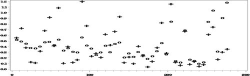
In the following four figures we show the results for and
,
for each area, with the areas ordered as above, starting with the area with the smallest number of complete responses.
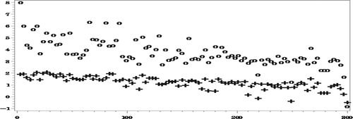
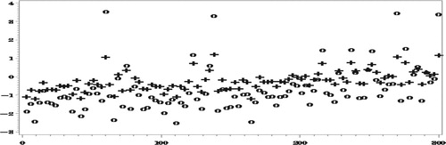
Figures and show how the proposed method reduces very significantly the bias due to NMAR nonresponse. As expected, the bias of both set of predictors decreases as the number of complete responses increases but our proposed predictors are seen to be much less biased.
Figure 1. of
(‘o’) and
(‘+’).
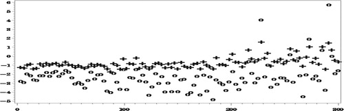
Figure 2. of
(‘o’) and
(‘+’).
The reduction in RelRMSE by accounting for the NMAR nonresponse in Figure is not big, which is explained by the fact that the bias of the predictors that ignore the nonresponse is not very high in this case. Notice in this respect that the average number of missing values over the 500 simulations is 5531.5, compared to an average number of 6014.6 missing values of
. Nonetheless, when averaging the
over all the areas we find that,
When estimating
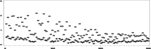
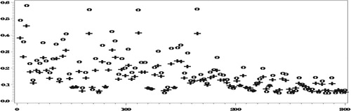
in Figure , the reduction in the
by use of the proposed procedure is much more drastic, particularly in the areas with small numbers of complete responses, due to the large bias when ignoring the NMAR nonresponse.
Next, we study the sensitivity of the proposed approach to correct specification of the response model. For this, we repeated the same simulation study, but by computing the response probabilities as:
(11)
(11)
with the same coefficients as in (10).
Figure 3. of
(‘o’) and
(‘+’).
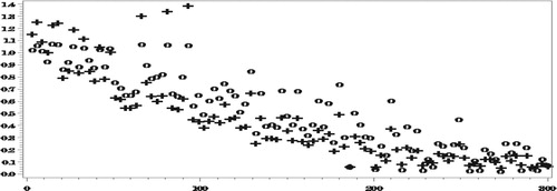
Figure 4. of
(‘o’) and
(‘+’).
With these response probabilities, the number of complete responses in an area (averaged over the 500 simulations), is in the range [9.3, 18.3].
When estimating the response model parameters in Step S5 of the simulation, we still use the model (10) as the working model, so that the model for the response is misspecified, and so is the model estimated for the missing data. (As mentioned before, the model estimated for the completely observed outcomes is also not correct).
Table compares the true response probabilities (Equation (11)) with the average of the estimated response probabilities over the 500 simulations under the misspecified response model (Equation (10)). Notice that except in a few cases, the averages of the estimated response probabilities under the misspecified model are close to the true response probabilities, already illustrating lack of sensitivity of our proposed approach to correct specification of the response model, although the differences between the true response probabilities and their estimates are occasionally larger for any given sample.
Table 2. True response probabilities, , and average of estimated response probabilities, under misspecified response model, for different response patterns .
As seen in Figures and , with the misspecified response model (and the model for the completely observed data), there are no big biases even when ignoring the NMAR nonresponse. Nonetheless, even in this case, when averaging over all the areas, ,
,
,
.
Figure 5. of
(‘o’) and
(‘+’), response model misspecified.
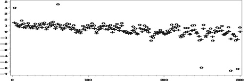
Figure 6. of
(‘o’) and
(‘+’), response model misspecified.
Next we compare the RelRPMSEs of the two estimators.
Figures and show reduction in the RelRPMSEs when accounting for the NMAR nonresponse in the areas with small number of complete responses. When averaging over all the areas,
We conclude that even under the misspecified models, our approach generally yields predictors with smaller RelRMSEs than when ignoring the NMAR nonresponse (Figures and ). Clearly, the predictors obtained under this approach have larger variances than when ignoring the NMAR nonresponse, due to all the complex computations involved, so that the large differences in the bias do not always translate into corresponding large differences in the RelRMSEs.
Figure 7. of
(‘o’) and
(‘+’), response model misspecified.
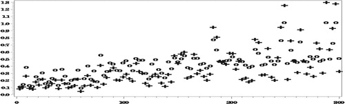
Figure 8. of
(‘o’) and
(‘+’), response model misspecified.
Finally, we report the results of RelRPMSE estimation. Due to time limitation, the results so far are based on only 100 parent samples and 50 bootstrap samples for each parent sample. Figures and compare the ‘true’ (empirical) RelRPMSEs over the 100 parent samples, with the mean of the corresponding bootstraps estimates.
Figure 9. of
(‘+’), and bootstrap estimates (‘o’).
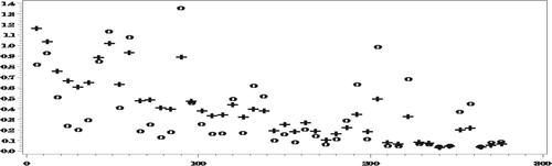
Figure 10. of
(‘+’), and bootstrap estimates (‘o’).
The results in Figures and show for most areas good performance of the bootstrap estimators and we believe that with more parent samples and bootstrap samples, the results will look even better. Even with the current runs, when averaging over all the areas,
illustrating the unbiasedness of the bootstrap estimators when averaging over all the areas.
We compared the empirical RelRPMSE’s with the bootstrap estimates also for the case of the misspecified response model and obtained similar results. To save in space, we don’t show the corresponding figures.
6. Summary
In this paper we propose a general approach for multivariate SAE under NMAR nonresponse within the selected areas. The approach consists of fitting a model for the observed data and using this model for estimating a postulated multivariate response model by application of the missing information principle. Once the response model is estimated, we derive the model holding for the missing data, which is used for imputing the missing data, thus obtaining a complete file of sample data that is used for estimating the unknown small area parameters. A bootstrap procedure is proposed for estimating the root prediction mean squared errors of the small area predictors, which consists of generating a pseudo population with similar behaviour to the behaviour of the true underlying population, and selecting many samples from the pseudo population and many sets of responses for each sample.
A simulation study shows good performance of our approach in terms of point and RPMSE estimation. The simulation study also illustrates certain robustness to misspecification of the response model. The empirical study in this paper considers the case where the models that are fitted for the responding units and the response probabilities are logistic, but the theoretical derivations assume general models for the observed data and the response mechanism. Thus, we encourage researchers of SAE to apply the procedure to simulated and real data sets, with possibly different models assumed for the observed data and the response probabilities.
Disclosure statement
No potential conflict of interest was reported by the authors.
Additional information
Notes on contributors
Danny Pfeffermann
Danny Pfeffermann is currently the National Statistician and General Director of the Central Bureau of Statistics of Israel. His main research areas are analytic inference from complex sample surveys and in particular, informative samples with non-ignorable nonresponse, small area estimation, seasonal adjustment and trend estimation and recently, accounting for mode effects and proxy surveys.
Michael Sverchkov
Michael Sverchkov is a Research Mathematical Statistician at the US Bureau of Labor Statistics. His main research areas are analytic inference from complex sample surveys and in particular, informative samples with non-ignorable nonresponse, small area estimation, seasonal adjustment.
Notes
* The opinions expressed in this paper are of the authors and do not necessarily represent the policies of the U.S. Bureau of Labor Statistics and the Israel Central Bureau of Statistics.
References
- Cepillini, R., Siniscialco, M., & Smith, C. A. B. (1955). The estimation of gene frequencies in a random mating population. Annals of Human Genetics, 20, 97–115. doi: 10.1111/j.1469-1809.1955.tb01360.x
- Little, R. J. A. (1982). Models for nonresponse in sample surveys. Journal of the American Statistical Association, 77, 237–250. doi: 10.1080/01621459.1982.10477792
- Little, R. J. A., & Rubin, D. B. (2002). Statistical analysis with missing data (2nd ed.). New York: Wiley.
- Orchard, T., & Woodbury, M. A. (1972). A missing information principle: Theory and application. Proceedings of the 6th Berkeley Symposium on Mathematical Statistics and Probability, 1, 697–715.
- Pfeffermann, D., & Sikov, N. (2011). Imputation and estimation under nonignorable nonresponse in household surveys with missing covariate information. Journal of Official Statistics, 27, 181–209.
- Pfeffermann, D., & Sverchkov, M. (2007). Small-area estimation under informative probability sampling of areas and within selected areas. Journal of the American Statistical Association, 102, 1427–1439. doi: 10.1198/016214507000001094
- Riddles, K. M., Kim, J. K., & Im, J. (2016). A propensity-score adjustment method for nonignorable nonresponse. Journal of Survey Statistics and Methodology, 4, 215–245. doi: 10.1093/jssam/smv047
- Rubin, D. B. (1976). Inference and missing data. Biometrika, 63, 581–590. doi: 10.1093/biomet/63.3.581
- Sverchkov, M. (2008). A new approach to estimation of response probabilities when missing data are not missing at random. Joint statistical Meetings. Proceedings of the section on survey research methods (pp. 867–874).
- Sverchkov, M., & Pfeffermann, D. (2004). Prediction of finite population totals based on the sample distribution. Survey Methodology, 30, 79–92.
- Sverchkov, M., & Pfeffermann, D. (2018). Small area estimation under informative sampling and not missing at random nonresponse. Journal of the Royal Statistical Society JRSS-SA, 181, 981–1008. doi: 10.1111/rssa.12362
Appendix. Illustration of the use of Equation (6) for Estimation of the response probabilities:
Mixed logistic model for the outcome variables with a single covariate.
Consider bivariate variables , and suppose that the model fitted to the observed data of the respondents is the mixed generalised logistic model,
(A1)
(A1)
Suppose a generic response model,
=
.
We assume that and
are independent given
, and that
.
Then, for example, for , the components of (6) can be written as,
Similar expressions are obtained for and
.