Using state space models as a statistical impact measurement of survey redesigns: a case study of the labour force survey of the Australian Bureau of Statistics

ABSTRACT

The goals of any major business transformation programme in an official statistical agency often include improving data collection efficiency, data processing methodologies and data quality. However, the achievement of such improvements may have transitional statistical impacts that could be misinterpreted as real-world changes if they are not measured and handled appropriately.

This paper describes a development work that sought to explore the design and analysis of a times-series experiment that measured the statistical impacts that sometimes occur during survey redesigns. The Labour Force Survey (LFS) of the Australian Bureau of Statistics (ABS) was used as a case study. In the present study:

1. A large-scale field experiment was designed and conducted that allowed the outgoing and the incoming surveys to run in parallel for some periods to measure the impacts of any changes to the survey process; and

2. The precision of the impact measurement was continuously improved while the new survey design was being implemented.

The state space modelling (SSM) technique was adopted as the main approach, as it provides an efficient impact measurement. This approach enabled sampling error structure to be incorporated in the time-series intervention analysis. The approach was also able to be extended to take advantage of the availability of other related data sources (e.g., the data obtained from the parallel data collection process) to improve the efficiency and accuracy of the impact measurement. As stated above, the LFS was used as a case study; however, the models and methods developed in this study could be extended to other surveys.

KEYWORDS:

• Intervention analysis
• survey sampling
• structural time series modelling
• labour force
• survey
• Kalman filter

1. Introduction

It is common practice for national statistical offices to employ a repeated sampling scheme. This practice enables changes in the total aggregate (or population) and different cross-sections to be estimated. The time series produced under a repeated survey scheme over time creates a basis for social, economic, environmental analysis and policy making.

Any changes to a survey process could potentially have a systematic effect on the outcomes of a survey. Such systematic differences are referred to as discontinuities or impact and affect the continuity of the estimated time series obtained by a repeated survey. This creates difficulties for users in interpreting movements in the data when making policy decisions, as it may not be clear if the period-to-period change in the estimates represent real-world changes or if they are the result of differences in measurement biases introduced by the changeover to a new survey design. Thus, any changes in survey methodology have to be well managed. Further, the effects of methodological change need to be identified, measured and adjusted, if necessary, to provide a coherent picture before and after the change and to mitigate the risk of the changes being misinterpreted.

The Australian Bureau of Statistics (ABS) is embarking on a transformation programme, which includes, among other changes, the application of different collection modes for survey data and the use of different, but more efficient, sampling frames and estimation methods for official statistics. This transformation is expected to deliver positive changes to official statistics; however, there is a risk that such changes could have a statistical impact on some ABS time series. Consequently, methodologies need to be developed to measure, and where necessary adjust for, statistical impacts.

The first and the most straightforward approach to assessing the effects of survey changes is to conduct times-series experiments. In such experiments, data are collected under the old (control) and new (treatment) survey approach simultaneously. Preferably, such data should be based on randomised experiments. The data can be used to obtain a direct accurate estimate of the impacts, depending on the size of the available sample at one survey period and the number of periods. In the present paper, this approach is referred to as a parallel run (see, for example, Van den Brakel, 2008).

Various intervention analyses of time-series models have also been widely used to measure possible time-series discontinuities with or without using the information from a parallel run. For example, Glass, Willson, and Gottman (2008) provide a general framework of the methodological aspects of control groups in time series. Similarly, in Chapter §8.6, Harvey (1989) also provides a general Seemingly Unrelated Time Series Equations (SUTSE) model for intervention analysis with control groups, while Van den Brakel and Krieg (2015) describe how they used multivariate STM to measure the statistical impact induced by the Dutch Labour Force Survey (LFS) redesign. Van den Brakel et al. (2017, Van den Brakel, Zhang, & Tam, 2019) also described a general framework for a statistical impact measurement (SIM).

In this paper, we explore a number of impact measurement strategies that could be applied to surveys redesigns, such as that planned for the Australian LFS. In relation to the parallel-run design, this paper primarily focused upon a methodology that could ascertain the pre-determined statistical accuracy of the minimum detectable impact (MDI) (in terms of Type I and II errors). State space modelling (SSM) techniques were used to address some special characteristics of the ABS LFS.

Section 2 of this paper provides a brief introduction to the characteristics of the current ABS LFS survey, outlines possible future changes and considers the options for measuring statistical impact. Section 2 also considers a number of general STMs and their state space presentation for measuring statistical impact. Section 3 describes the methods and models that could be used for the LFS parallel-run design and discusses the simulated results. Section 4 evaluates a number of options and suggests a hybrid option to balance different priorities in terms of costs, accuracy and revisions. Finally, Section 5 discusses the implications of different options and avenues for future research.

All the calculations reported in this paper were undertaken using programmes written in the SSM procedure in software packages: SAS, SsfPack (see Koopman, Shephard, & Doornik, 2008) and R.

2. Australian Bureau of Statistics labour force survey

2.1. Australian Bureau of Statistics labour force survey design

The LFS is based on a multi-stage area sample of dwellings and covers approximately 0.32% of the civilian population of Australia aged 15 years and over (ABS, 2016). Households selected for the LFS are interviewed using face-to-face, telephone or web forms each month for eight consecutive months and one-eighth of the sample is replaced each month. The LFS sample can be thought of as comprising eight sub-samples (or rotation groups [RGs]). Each RG remains in the survey for eight months; one RG is ‘rotated out’ each month and replaced by a new group that is ‘rotated in’. This high overlap of respondents from month-to-month induces strong serial correlations in the sampling errors.

A composite estimator is used to obtain monthly estimates for the employed and unemployed labour force (Bell, 2001). This estimator combines the monthly general regression (GREG) estimates for the eight waves observed in the last six months into an approximate design unbiased estimate for the current month.

2.2. Options for measuring statistical impacts

As part of the present study, three general options (discussed further below) were examined in relation to the precision of the SIM, the risks and the costs related to the practical implementation.

Option A: A 100% control sample to maintain the production quality of the current LFS during the parallel run. This option would enable optimal combinations of the treatment sample size and length of parallel run to be ascertained. This option would have the lowest levels of risk for the continuation of the official publications but would be costly.

Option B: Reduce the size of the control sample and make the treatment sample size equal to the control sample size (e.g., have a control group and a treatment group equal to 75% of the regular sample size of the current LFS). Such a balanced design would enable the statistical impact to be estimated as precisely as possible; however, this would be done at the cost of accepting less precise and less regular LFS estimates for official publication purposes during the parallel-run period. Additionally, this option might not be accepted by external users due to the increase of sampling errors in the regular survey estimates.

Option C: Phase-in a new process where by one group is rotated in each month. After 8 months, the existing process could be fully changed to reflect the new process. This strategy would not allow for a period of parallel data collection; thus, the SIM would rely fully on a times-series model to estimate the statistical impact. A potentially large revision may result and have to be accepted after the changeover had begun. This option carries the highest risks.

Finally we propose a hybrid option. This combines the information obtained with a small parallel run with the information observed before and after the parallel run with a structural time series model. The information obtained with the parallel run is used as a-priori information in the time-series model. The observations obtained before and after the parallel run are in the time-series model used to further improve the precision of the initial estimate for the discontinuity obtained with the parallel run. The details are explained in Subsection 4.2.

2.2.1. Reasons for measuring statistical impact using general regression estimates at the rotation group level

Our main objective was to measure the statistical impact at the level of composite estimates. The composite estimator applied in the ABS LFS combines monthly GREG estimates for the eight waves over the last six months. Consequently, any abrupt statistical impact at the current end of the series due to the changeover to a new design should be smoothed out over a longer period. To avoid such an effect and to achieve an accurate and timely SIM, the statistical impact was measured at the monthly GREG estimates in the separate rotation group levels. The corresponding impacts to the composite LFS estimates were then derived accordingly.

A number of potential changes to the LFS must be considered and their statistical impacts assessed. It would be unrealistic to assume that a statistical impact would be uniformly equal across all waves, as the proposed changes may have different impacts on different waves. Such differences are referred to as ‘wave sensitive’ differences in this paper. For example, the use of e-collection as the primary collection mode could produce changes in respondent induction and the strategy for promoting web-form adoption could potentially lead to a wave sensitive effect.

2.3. Using structural time-series models at the rotation group level to measure statistical impact

Assume ${\hat{y}}_{i,t}$ is a GREG estimate of the main LFS variables (e.g., number of employed persons and number of unemployed persons from the rotation group that in the current month t has been observed i times [i = 1, … 8]) (referred to hereafter as ‘wave i’). Without losing generality, the structural measurement errors for the wave i at time t are:

1. time invariant rotation group bias (RGB) $b_i$ for wave i; and

2. sampling error, $e_{i,t}$ for wave i in period t.

The rotation group bias, $b_1,\dots ,b_8$, showed a permanent wave sensitive level shift (LS) compared to the reference wave (in this study, Wave 7 was the reference wave; thus, without loss of generality, we set $b_7=0$).¹ The following equation (Pfeffermann, 1991) describes the relationship between an observed estimate, ${\hat{y}}_{i,t}$ and the unobserved components, y_t, $b_i$, $e_{i,t}$ and ${\alpha }_i$. In this paper, all the modelling work uses a logarithmic scale. Thus, the additive components are multiplicative in the original scale. Standard Error (SE) is equivalent to Relative Standard Error (RSE) in the original scale. It should be noted that these terms are used interchangeably in this paper. Thus: (1) $\left(\begin{array}{c}{\hat{y}}_{1,t}\\ ⋮\\ {\hat{y}}_{8,t}\end{array}\right)=1_{\left[8\right]}{y}_t+\left(\begin{array}{c}{b}_1\\ ⋮\\ b_8\end{array}\right)+\left(\begin{array}{c}{e}_{1,t}\\ ⋮\\ e_{8,t}\end{array}\right)$(1) where y_t is a true population value, $1_{\left[8\right]}$ is the eight-dimensional vector with elements equal to one.

The target variable, $y_t$, can be expressed by a STM: (2) $y_t=T_t+S_t+I_t,$(2) where T_t, S_t, and I_t denote the smooth trend model, the seasonal model and the irregular component, which is often assumed to be white noise that represents unexplained variations in the population parameter (see Durbin & Koopman, 2012 for further details). The sampling error stochastic process, $e_t$ can be modelled as white noise for Wave 1 (assuming there was no correlations with estimates from the previous panel): (3) $e_{1,t}=u_{1,t},u_{1,t}\cong NID\left(0,{\sigma }_{1,u}^2\right)$(3) as an AR(1) process for Wave 2 (4) $e_{2,t}={\phi }_{2,1}{e}_{1,t-1}+u_{2,t},u_{2,t}\cong NID\left(0,{\sigma }_{2,u}^2\right)$(4) and as an AR(2) process for the other waves (i = 3, 4, … 8) (5) $\begin{array}{rl}{e}_{i,t}& ={\phi }_1{e}_{i-1,t-1}+{\phi }_2{e}_{i-2,t-2}+u_{i,t},\\ u_{i,t}& \cong NID\left(0,{\sigma }_{i,u}^2\right)\end{array}$(5) where coefficients ${\phi }_1$ and ${\phi }_2$ and the sampling error disturbance variance, ${\sigma }_u^2$, can be pre-defined with the LFS data (see Pfeffermann, Feder, & Singnorelli, 1998).

3. A parallel-run design

3.1. Design considerations in the labour force survey context

The objectives of any LFS parallel-run design are to:

• measure the direct statistical impacts induced by the ABS process change to the published ABS LFS outputs;

• identify statistical impacts in a timely manner to support statistical risk management; and

• obtain an accurate SIM with a minimum treatment sample for the agreed accuracy level and a feasible parallel-run design.

3.1.1. Working assumptions

For this study, the following hypothetical accuracy criterion² was set to detect a significant statistical impact: One SE of population³ estimates (43,750 and 19,500 employed and unemployed persons, respectively) with conventional Type I and II errors less than 5% and 50%, respectively.

The MDI was defined as the minimum size of the impact, $\alpha$, that could be detected based on the above stated accuracy criterion. Its value was calculated as the SE of the estimated statistical impact, $SE\left(\hat{\alpha }\right)$, times a multiplier, which was derived from the predefined Type I and II errors. The multiplier of 1.96 corresponds to Type I and II errors of 5% and 50%, respectively.

The ratio of the MDI to one SE of the population estimate, $SE\left(\hat{y}\right)$ (the MDI ratio), $1.96\times SE\left(\hat{\alpha }\right)/SE\left(\hat{y}\right)$, indicates that a SIM method is successful when its value is less than or equal to one. The MDI ratio provides a uniform measure and makes comparisons of the SIMs of different variables easier.

The SIM, as described in this study, was primarily designed to identify a permanent LS induced by a new LFS design with additional consideration of sampling error properties.

The following two parameters for a parallel-run design must meet the accuracy criterion and operational feasibility:

1. The size of the treatment sample; and

2. The duration of the parallel run.

From an operational feasibility perspective, the duration of any parallel run in this study was limited to less than two years.

3.2. State space model formulation

Equations (1–5) describe a general SSM framework for GREG estimates of the LFS at the rotation group level with interventions. With or without a control group, this model reflects a common approach in the literature (Harvey, 1989) that is used to measure the statistical impact as the intervention component. However, such a conventional model has to estimate many hyper-parameters, as it needs to estimate the ‘true’ population, y_t, in the STM Equation (2). Basically, the differences between the model’s predicted value and observed value provide a source for measuring the statistical impact. Such relatively complicated model identification and prediction can be vulnerable to rapid real-world changes. Further, the model may be unable to account for rapid real-world changes during the parallel-run period. As the sole goal of this study was to estimate the statistical impact rather than produce a ‘true’ population estimate, the model was simplified for the parallel-run scenario.

In the case of the LFS, the existing composite estimator continued to be used to produce the ‘true’ labour force population estimates. Consequently, the conventional intervention analysis was simplified by modelling the differences between the estimates produced under the current design and the estimates produced under the new design conducted in parallel. This reduced the risks of rapid changes or outliers affecting the estimation and improved robustness by reducing model complexity. The difference SSM for estimating statistical impact is developed further below.

3.2.1. The conceptual decomposition of a statistical impact on the general regression estimate

Suppose a new LFS design (n) starts from time $t_1$. Then model (1) can be extended for the observations obtained at months $t\ge t_1$ by adding a vector that contains level shifts for the separate waves to model the systematic difference due to the change-over to a new survey design. This results into the following model: (6) $\left(\begin{array}{c}{\hat{y}}_{1,t}^{\left(n\right)}\\ ⋮\\ {\hat{y}}_{8,t}^{\left(n\right)}\end{array}\right)=1_{\left[8\right]}{y}_t+\left(\begin{array}{c}{b}_1\\ ⋮\\ b_8\end{array}\right)+\left(\begin{array}{c}{\alpha }_1{x}_{1,t}\\ ⋮\\ {\alpha }_8{x}_{8,t}\end{array}\right)+\left(\begin{array}{c}{e}_{1,t}^{\left(n\right)}\\ ⋮\\ e_{8,t}^{\left(n\right)}\end{array}\right)$(6) where ${\hat{y}}_{i,t}^{\left(n\right)}$ denotes the new GREG estimate for wave i, $e_{i,t}^{\left(n\right)}$ is sampling error of the new LFS design and $x_i$ is an intervention dummy variable denoted as $\begin{array}{rl}{x}_{i\text{,}t}& =\left\{\begin{array}{ll}\text{1,}& \text{if observations are obtained under}\\ & \text{the new design of wave }i\text{ at time }t\text{,}\\ \text{0,}& \text{otherwise}\text{. }\end{array}\right.\end{array}$The regression coefficients, α_i, are the LSs induced by the redesign of the survey process and are the measurement of the statistical impact (Van den Brakel & Roels, 2010; Van den Brakel, Smith, & Compton, 2008). To identify the model, the LSs and the coefficients for the RGB were assumed to be time invariant.⁴

In the case of a parallel run, the statistical impact for each wave is obtained by taking the difference between (6) and (1): (7) $\underset{\text{difference in estimates}}{\underbrace{\left(\begin{array}{c}{\hat{y}}_{1,t}^{\left(n\right)}-{\hat{y}}_{1,t}\\ ⋮\\ {\hat{y}}_{8,t}^{\left(n\right)}-{\hat{y}}_{8,t}\end{array}\right)}}=\underset{\text{difference in RGB}}{\underbrace{\left(\begin{array}{c}{\alpha }_1{x}_{1,t}\\ ⋮\\ {\alpha }_8{x}_{8,t}\end{array}\right)}}+\underset{\text{difference in SE}}{\underbrace{\left(\begin{array}{c}{e}_{1,t}^{\left(n\right)}-e_{1,t}\\ ⋮\\ e_{8,t}^{\left(n\right)}-e_{8,t}\end{array}\right)}}$(7) The structural changes come from:

1. A permanent LS presented in the ‘difference in RGB’; and

2. A dynamic sampling error change presented in the ‘difference in SE’.

The ‘true’ population $y_t$ cancels out under the difference model formulation and was thus excluded from the estimation.

3.2.2. Estimating the statistical impact during a parallel run

In practice, a new design will usually be introduced by each successive rotation group. Assuming a parallel run is conducted for $t_0\le t<t_1$ a new series ${\hat{y}}_t^{\left(\tau \right)}$ can be constructed⁵ as: (8) $\begin{array}{r}{\hat{y}}_{i,t}^{\left(\tau \right)}=\left\{\begin{array}{ll}{\hat{y}}_{i,t}^{\left(n\right)}& t_0\le t<t_1\text{ and wave }i\\ & \text{ has a treatment sample}\\ {\hat{y}}_{i,t}& \text{otherwise }\end{array}\right.,\\ i=1,\dots ,8\end{array}$(8) (9) ${\hat{y}}_{i,t}^{\left(\tau \right)}=y_t+b_i+{\alpha }_i{x}_{i,t}+e_{i,t}+\left(e_{i,t}^{\left(n\right)}-e_{i,t}\right)x_{i,t}$(9) with an intervention dummy variable $x_{i,t}$ (10) $x_{i,t}=\left\{\begin{array}{ll}1& t_0\le t<t_1\text{ and wave }i\\ & \text{ has a treatment sample}\\ 0& \text{otherwise }\end{array}\right.$(10) Thus, the permanent LS ${\alpha }_i$ for Wave $i$ can be estimated from the parallel run with a combined sampling error process ${\eta }_{i,t}=e_{i,t}^{\left(n\right)}-e_{i,t}$: (11) ${\hat{y}}_{i,t}^{\left(\tau \right)}-{\hat{y}}_{i,t}^{}={\alpha }_i{x}_{i,t}+{\eta }_{i,t}{x}_{i,t}{t}_0\le t<t_1$(11) Assuming the sample rotation design continues, both $e_{i,t}$ and $e_{i,t}^{\left(n\right)}$ follow the same Auto-Regressive (AR) model (see Equations [3–5]) process, but with a different disturbance variance, ${\sigma }_{\eta ,\delta }^2$. Thus: (12) $\begin{array}{rl}{\eta }_{i,t}& ={\phi }_1{\eta }_{i,t-1}+{\phi }_2{\eta }_{i,t-2}+{\delta }_{i,t}\\ {\delta }_{i,t}& \cong NID(0,{\sigma }_{i,\delta }^2)\end{array}$(12) (13) $\begin{array}{rl}{\sigma }_{i,\delta }^2& ={\sigma }_{i,(e,u)}^2+{\sigma }_{i,(e^{\left(n\right)},u)}^2\\ & -2corr(e_{.,.}^{\left(n\right)},e_{.,.}){\sigma }_{i,(e,u)}{\sigma }_{i,(e^{\left(n\right)},u)}\end{array}$(13) ${\phi }_1$, ${\phi }_2$ and ${\sigma }_{i,(e,u)}^2$ can be estimated from the existing LFS sample design. ${\sigma }_{i,(e^{\left(n\right)},u)}^2$ can be determined by the new treatment sample design. A more accurate estimate of ${\alpha }_i$ from Equations (11) and (12) can be achieved by maximising correlation $\rho =corr\left(e_{.,.}^{\left(n\right)},e_{.,.}\right)$ in Equation (13). This relies on the working assumptions made earlier; that is, that the existing and new LFS designs have the same sampling error stochastic process (i.e., the same autoregressive coefficients of the AR(2) model). Thus, ${\sigma }_{i,\delta }^2\approx ({\sigma }_{i,(e^{\left(n\right)},u)}-{\sigma }_{i,(e,u)}{)}^2$ when $\rho \approx 1$.

The difference between the RGB of the existing design and new design can be estimated from the following state space model presentation.

The observation equation is: (14) ${\hat{y}}_{i,t}^{\left(\tau \right)}-{\hat{y}}_{i,t}^{}={\alpha }_i{x}_{i,t}+{\eta }_{i,t}{x}_{i,t}i=1,\cdots ,8$(14) The state equation is:⁶ (15) $\left(\begin{array}{c}{\mathit{\eta }}_{\mathbf{\text{t}}}\\ {\mathit{\eta }}_{\mathbf{\text{t}}-1}\end{array}\right)=\left(\begin{array}{cc}{\mathrm{\Theta }}_1& {\mathrm{\Theta }}_2\\ \mathbf{\text{I}}& \mathbf{\text{0}}\end{array}\right)\left(\begin{array}{c}{\mathit{\eta }}_{\mathbf{\text{t}}-1}\\ {\mathit{\eta }}_{\mathbf{\text{t}}-2}\end{array}\right)+\left(\begin{array}{c}{\mathit{\delta }}_{\mathbf{\text{t}}}\\ \mathbf{\text{0}}\end{array}\right)$(15) Where $\begin{array}{rl}{\mathit{\eta }}_t& =({\eta }_{1,t},{\eta }_{2,t},\dots ,{\eta }_{8,t}{)}^{\mathrm{\prime }},{\mathit{\delta }}_t=({\delta }_{1,t},{\delta }_{2,t},\dots ,{\delta }_{8,t}{)}^{\mathrm{\prime }},\\ {\mathbf{\Theta }}_1& =\left(\begin{array}{cc}{{\mathbf{0}}^{\mathrm{\prime }}}_{\left[7\right]}& 0\\ {\phi }_1{\mathbf{I}}_{\left[7\right]}& {\mathbf{0}}_{\left[7\right]}\end{array}\right),{\mathbf{\Theta }}_2=\left(\begin{array}{cc}{\mathbf{0}}_{[2\times 6]}& {\mathbf{0}}_{[2\times 2]}\\ {\phi }_2{\mathbf{I}}_{\left[6\right]}& {\mathbf{0}}_{[6\times 6]}\end{array}\right).\end{array}$${\mathbf{0}}_{\left[j\right]}$ is a j-dimensional vector with each element equal to zero, ${\mathbf{0}}_{[p\times q]}$ a p × q matrix with each element equal to zero, and ${\mathbf{I}}_{\left[j\right]}$ is a j × j identity matrix.

3.2.3. An analytical solution for the parallel-run parameters

The estimated coefficients ${\hat{\alpha }}_i(i=1,\cdots ,8)$ are the permanent LSs and the RGB of the new LFS design can be derived by $b_i+{\hat{\alpha }}_i(i=1,\cdots ,8)$, where $b_i$ is the RGB of the existing LFS design.

The null hypothesis for no statistical impact is H₀: ${\alpha }_i=0(i=1,\cdots ,8)$. Based on classical statistical theory, we sought to determine the sample size needed to test whether the mean of the treatment samples differed to the means of the control samples where the control was regarded as the true value and the difference was the statistical impact.

The variance of the sampling error disturbance ${\sigma }_{i,\mu }^2$ from Equations (12) and (13) was rewritten as: (16) $\begin{array}{rl}{\sigma }_{i,\delta }^2& ={\sigma }_{i,(e,u)}^2+{\sigma }_{i,(e^{\left(n\right)},u)}^2-2\rho {\sigma }_{i,(e,u)}{\sigma }_{i,(e^{\left(n\right)},u)}\\ & ={\gamma }_i\left({\sigma }_{i,e}^2+{\sigma }_{i,e^{\left(n\right)}}^2-2\rho {\sigma }_{i,e}{\sigma }_{i,e^{\left(n\right)}}\right)\\ & ={\gamma }_i\left(\frac{1}{n_C}+\frac{1}{n_T}-\frac{2\rho }{\sqrt{n_C{n}_T}}\right){\sigma }^2\\ & ={\gamma }_i\left(1+\frac{1}{\kappa }-\frac{2\rho }{\sqrt{\kappa }}\right){\left(\frac{\sigma }{\sqrt{n_C}}\right)}^2\\ & ={\gamma }_i\left(1+\frac{1}{\kappa }-\frac{2\rho }{\sqrt{\kappa }}\right){\sigma }_{i,e}^2\end{array}$(16) where ${\sigma }_{i,e}^2$ and ${\sigma }_{i,e^{\left(n\right)}}^2$ are the variance of the control and treatment sampling errors of Wave i and $\kappa =n_T/n_C$ is the sample size ratio between treatment and control samples. Finally: $\begin{array}{rl}{\gamma }_i& =\left\{\begin{array}{ll}1,& i=1({\phi }_1=0,{\phi }_2=0)\\ 1-{\phi }_1^2,& i=2({\phi }_1\ne 0,{\phi }_2=0)\\ (1+{\phi }_2)[{(1-{\phi }_2)}^2& \\ -{\phi }_1^2\left]/\right(1-{\phi }_2),& i\ge 3({\phi }_1\ne 0,{\phi }_2\ne 0)\end{array}\right.\end{array}$was derived from the sampling error AR process.

With some algebras (for further details see Zhang, Van den Brakel, Honchar, Wong, & Griffiths, 2017), the SE of ${\alpha }_i$ can be derived at any point of time t: (17) $SE\left({\alpha }_i|\kappa \right)=SE\left({\delta }_{i,t}\right)={\sigma }_{i,\delta }=\sqrt{{\gamma }_i\left(\frac{1}{\kappa }+1-\frac{2\rho }{\sqrt{\kappa }}\right)}{\sigma }_{i,e}$(17) We can also derive that the improvement is the gain: (18) $\frac{SE\left({\alpha }_i|\kappa \right)}{{\sigma }_{i,e}/\sqrt{\kappa }}=\sqrt{{\gamma }_i\left(\text{1 }+\kappa -2\rho \sqrt{\kappa }\right)}$(18) in terms of the proportional reduction to the SE of ${\alpha }_i$ by considering the sampling error process and intra-cluster correlation using the SSM model. The smaller the gain value, the bigger the reduction of the SE. This gain decreases with increasing intra-cluster correlation $\rho$. Notably, when $\rho$ = 0 (there is no intra-cluster correlation), the gain is $\sqrt{{\gamma }_i(1+\kappa )}$. For example, when $\kappa$ = 0.5, then the gains are 0.64 and 0.96 for the employed and unemployed labour forces of the LFS, respectively.

For a parallel run, with a treatment sample over periods {T}, the SE of ${\alpha }_i$ is: (19) $\begin{array}{rl}SE\left({\alpha }_i|\kappa ,n\right)& =\sqrt{\frac{1}{n}{\sigma }_{i,\delta }^2}=\sqrt{\frac{{\gamma }_i}{n}\left\{\frac{1}{\kappa }+1-\frac{2\rho }{\sqrt{\kappa }}\right\}}{\sigma }_{i,e}\\ & \text{because}{\delta }_{i,t}\cong NID(0,{\sigma }_{i,\delta }^2)\end{array}$(19) where $n$ is the number of times that Wave i was observed over the periods of {T}.

3.3. Simulation study

Equation (17) provides a theoretical solution to determine the SE of the statistical impact {${\alpha }_i$}. It can be used to allocate the treatment sample size by optimising $n$ (the number of times each wave is included in the periods of a parallel run) and $\kappa$ (treatment sample size proportion to control sample size) to meet the statistical accuracy criteria with the predefined parameters, ${\gamma }_i$, $\rho$ and ${\sigma }_{i,e}$ (which are specific to the employed and unemployed estimates). For this simulation study, an equal sampling error was assumed for the eight waves; that is, ${\sigma }_{i,e}^2={\sigma }_e^2(i=1,\cdots ,8)$. The sampling error disturbance variance of Wave i, ${\sigma }_{\delta ,i}^2$ can be derived from ${\sigma }_{i,\delta }^2={\gamma }_i\left(1+\frac{1}{\kappa }-\frac{2\rho }{\sqrt{\kappa }}\right){\sigma }_e^2$.

A simulation study was undertaken with the following two objectives:

1. To verify whether the theoretical solution was correct, and

2. To evaluate the Kalman filter performance of the SSM on a relatively short time series derived from a parallel run.

Model (7) is proposed as a parsimonious SSM as a tool to analyse a short time series obtained with a parallel run. Generally, the Kalman filter requires a relatively long time series, particularly in the case of Model (1) and (6), which contain many nonstationary state variables that require a diffuse Kalman filter initialisation. Since Model (7) uses the contrasts between the new and old design as the input series, most of the nonstationary state variables cancel out at the cost of having a short series. One objective of the simulation is to investigate whether this approach is an alternative for the hybrid option, discussed in Subsection 4.2, where the information of the parallel run is used for an exact initialisation of the regression coefficients of the level shifts in the Kalman filter.

Due to operational constraints, only one treatment RG was able to be introduced each month. Figure 1 presents a 15-month parallel-run scheme; each treatment RG was run in parallel for a full eight (=15–17) months. The shaded cells represent treatment RGs.

Figure 1. A scheme for 15 months parallel run.

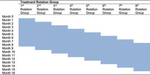
One hundred replicates were generated for different combinations of:

• parallel durations (11, 13, 15, and 19 months, where each separate wave was conducted in parallel for 4, 6, 8, and 12 months, respectively);

• treatment sample sizes ($\kappa$ = 30%, 50%, 80% and 100%); and

• intra-cluster correlations ($\rho$ = 0, 0.3, 0.5 and 0.8).

The RG level wave sensitive impacts {${\alpha }_i$} ($i=1,\cdots ,8$) were set for a combined impact size, $\alpha$, of one SE, $SE\left(\hat{y}\right)$, of the national LFS employment and unemployment, respectively (i.e., $\alpha =SE\left(\hat{y}\right)$). Appendix 1 describes how the simulated data at the RG level were generated for the simulation study.

This model is stationary with stability and observability. Thus, an unconditional mean and covariance were able to be used as the initial condition of the state variables (Aoki, 1987). Zhang et al. (2017) also showed that the analytical solution of the corresponding state correlation matrix can be derived as the sum of the serial cross-correlation of sampling errors {$e_i$}.

The following initialisations of the Kalman filter were used:

1. A diffuse initialisation for the state {${\alpha }_i$} with values of zero and large variances with a known correlation structure; and

2. An exact initialisation for the sampling error state {$e_i$} with zero expectations, estimated variance and zero correlations.

The SEs of {${\alpha }_i$} were estimated and were consistent over different waves (i = 1, 2, … 8) regardless of the true value of {${\alpha }_i$}. Thus, the precision of the impact estimates was not dependent on the size of the chosen impacts in the simulation.

The top panel of Figure 2 shows the average SE of ${\alpha }_i$ (avg.se⁷) against different combinations of intra-cluster correlation, (ρ), parallel-run duration, (n) and treatment sample size, (κ). The results were consistent with our expectations for both the employed and unemployed labour forces (i.e., the larger intra-cluster correlation or the longer parallel-run duration or larger the treatment sample size, the smaller of the SE of ${\alpha }_i$).

Figure 2. Average SE against treatment sample size, intra-cluster correlation and parallel duration.

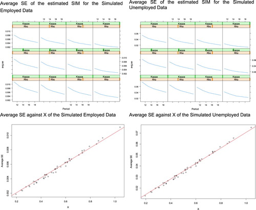
Variable $X=\sqrt{\frac{1}{n}\left(1+\frac{1}{\kappa }-\frac{2\rho }{\sqrt{\kappa }}\right)}$ was also created to examine its relationship with the SE of ${\alpha }_i$. The lower panel of Figure 2 shows the simulated results (dots) against the results (regression line) derived by regressing avg.se on X. This graphical presentation clearly demonstrates that there was a very strong linear relationship between avg.se and X.

Table 1 shows the regression analysis results. The high R-squre values (R²) values confirm that avg.se can be predicted from X.

Table 1. Average SE Regress on X.

	Employed	Unemployed
Coefficient of X	1.035e-02 (5.482e-05)	0.0706435 (0.0002898)
Null deviance	1.6335e-03	7.6127e-02
Residual deviance	2.1526e-06	6.0167e-05
R^2	0.9987	0.9992

From this analysis, it can be confidently concluded that the theoretical articulation of Equation (17) is correct. Thus, it appears that the Kalman filter performed well in estimating ${\alpha }_i$ with an expected SE.

In the context of the parallel-run design, from the structure of X, we confirmed that:

• Intra-cluster correlation is the most powerful variable in reducing the SE of estimated ${\alpha }_i$;

• The treatment sample size was the second most important variable. Notably, when the treatment sample size was the same as the control sample size (i.e., $\kappa$ = 1), this provided the most efficient balanced design for minimising the SE of the estimated ${\alpha }_i$; and

• The duration of the parallel run was the least powerful factor among the three to reduce the SE of the estimated ${\alpha }_i$.

The coefficients of X in Table 1 can be used with any combination of parallel-run duration, treatment sample size and intra-cluster correlation to predict the SE of ${\alpha }_i$ for both employed and unemployed persons in the LFS. Thus, an optimised parallel-run design was able to be achieved. However, the intra-cluster correlation between the control and treatment samples is usually unknown, unlike the sampling error and the rotation panel design induced AR sampling error dynamics, which can be estimated from the sample data (see Pfeffermann et al., 1998).

4. Evauation of the options for measuring statistical impact and change implementation

In this section, we evaluate the three different design options (described in Section 2) in relation to a parallel run based on the methodology developed in Section 3. The remainder of this section assesses the three options and proposes a hybrid option if an additional revision is acceptable 12 months after the introduction of a new LFS survey.

4.1. Evaluations of the three options

Using the formulae developed in Section 3, the parallel-run parameters can be calculated based on a given set of scenarios. As a new LFS design was hypothetical at this stage, it was assumed that the intra-cluster correlation between the control and treatment samples was zero (i.e., $\rho =0$). In relation to our simulation study, Table 2 shows the length of the parallel run required to meet the predefined accuracy criterion (see Section 3) for the unemployment scenarios of Option A with 100% and 50% treatment samples (A100 and A50, respectively) and Option B with 75% (B75) across both the control and treatment samples. It should be noted that none of the options appeared to meet the defined accuracy criterion with the operational feasibility constraints of a parallel run shorter than 24 months.

Table 2. Sample size and the length of the parallel run required for unemployment Options A and B.

	A100	A50	B75
Control sample size %	100	100	75
Treatment sample size %	100	50	75
SE on published estimates	Current	Current	1.15 times larger
Duration	32 months	>44	36 months
Risk	Low	Low	Moderate

Options A50 and B75 have the same total samples per month and their costs should be similar. However, B75 is a balanced design and is more efficient than A50 at measuring statistical impact. Thus, a shorter parallel run is sufficient; however, due to the sample size reduction for the control samples, the published LFS unemployment estimates during parallel-run periods are (1.15 times) more volatile.

In relation to the unemployment example with a 24-month parallel run, the estimated relative SEs of the statistical impacts for the composite estimates were 1.65%, 2.02% and 1.91% for each of the three options (A100, A50 and B75), respectively. These options detect a one SE (2.6%) statistical impact with a 5% Type I error and 53%, 64% and 61% Type II errors, respectively. The alternative interpretation may be that the three options can detect the size of the statistical impact of the MDI ratios 1.24, 1.52 and 1.43 times the current survey SE (2.6%) with the pre-defined precision.

The phase-in (i.e., Option C) implementation strategy did not use parallel data collection and was not designed for accurate SIM. This approach has a high risk, as there is limited opportunities to assess the impacts before implementation.

A one SE statistical impact is not detectable with the required accuracy within the 8-month phase-in period, as the statistical impact is wave sensitive and there are incomplete or insufficient observations of new samples. Table 3 shows our simulation results with a one SE statistical impact for the LFS unemployed (2.6%). In this table, the impact was measured at 3, 5 and 8 months for 100 replicates (there was an untested assumption of wave insensitive impact; that is, that the impact was uniform to all the waves).

Table 3. Total level shift detected by SSM across 100 replicates (Unemployed).

Periods after the first new design rotation group is introduced (month)	Overall impact %	MDI ratio
Simulated	2.60
3	1.86	4.1
5	2.23	4.0
8	2.34	3.9

The estimated impacts at 3 and 5 months (1.856% and 2.232%, respectively) were obviously not accurate (given that the true impact was 2.6%). The MDI ratio indicates that an impact greater than 3.9 SEs in the unemployed population estimate can be detected with the required precision. In such circumstances, there are two choices as to how the situation can be addressed if only this option is applied:

1. Ignore the impact, as the measured impact cannot meet the accuracy criterion. However, the statistical impact will appear in the published estimates and could be misinterpreted as real-world changes; or

2. Apply an ad-hoc manual adjustment based on the estimated impact. This action is not scientific and could potentially be subject to large revisions later⁸

Neither of these choices were deemed acceptable. Therefore, the phase-in represents a very high risk option.

Table 3 also shows that the estimated impact is close to the real impact after the end of the phase-in (i.e., at 8 months). However, the impact cannot be measured accurately even after 24 months. Further information is provided in the next sub-section.

4.2. Simulation studies for different options and a hybrid option

The advantage of a large parallel run (i.e., Option A) is that such an approach minimises the risks related to regular publications during the changeover. If unexpected results are observed using the new process during the parallel run, the old approach could still be adopted. Further, as a large parallel run can estimate the statistical impact directly and with high precision, another advantage of this option is that it facilitates the implementation of the new survey without further revision of the impact measurements after the changeover. However, this approach is expensive, as significant data collection effort is required.

The opposite approach (i.e., Option C) involves no parallel run and requires a times-series model be used to estimate the impact. The major advantages of this approach include that it is inexpensive and avoids the additional fieldwork that would be required by a parallel run. However, skipping a period of parallel data collection and relying on a times-series model to estimate the statistical impact also has several disadvantages and risks. First, it is not clear in advance if the times-series estimates for the statistical impact will have the required levels of precision. Further, any estimates of the impact could be unreliable directly after the changeover and will likely have to be revised after new observations become available under the new survey design. Consequently, revisions must be expected and accepted. Implementing the changeover without a period of parallel data collection also increases risks during the changeover. If the new survey design is a failure or has a significant impact, the old approach will have to be adopted; however, if this occurs, there will be a period for which no data or less reliable data are available for the production of official statistics.

An intermediate option is to have a small parallel run and combine the information derived from this run with the adoption of a times-series modelling approach. For example, a parallel run could be conducted with 20% or 50% of the regular sample size for a period of 12 months. The results obtained from the parallel run could be used as a-priori information in the times-series model. This could be done by using the direct estimates for the impact and their SEs obtained with the parallel run as initial values for the state variables of the interventions in the Kalman filter. As an alternative, the parallel run could be analysed with SSM Equation (7) and these results could be used as a-priori information in the times-series model. The information from the time series observed before the start of the parallel run and the information that becomes available under the new approach after finalising the parallel run could be used in the times-series model to further improve the precision of the impact estimates. It should be noted that this option directly reduces the risk of having a period without official figures after the changeover and also reduces the amount of revisions.

As per the simulation approach described in Section 3.2, more simulations for the national unemployed and employed persons from the rotation group level estimates were conducted to illustrate the precision of the impact estimates.⁹ The simulations were run using the times-series model approach without a parallel run and with five different parallel-run scenarios of reduced sample sizes (see Table 4). The SEs in Table 4 refer to the statistical impact estimates at the rotation group level obtained with the control sample, the treatment sample and the specified parallel-run periods. The sample size percentages refer to the current sample size of the regular LFS. The MDI ratios were calculated for the overall composite estimates.

Table 4. Different parallel-run scenarios used in the simulation^a.

	Sample size			Unemployed			Employed
				Standard error			Standard error
Scenario	Control sample	Treatment sample	Parallel-run period month	% points	total	MDI ratio	% points	total	MDI ratio
1	100%	20%	18	7.9	61,620	4.05	1.08	135,000	5.25
2	100%	50%	12	5.6	43,680	2.87	0.81	101,250	3.94
2	100%	20%	24	5.6	43,680	2.87	0.81	101,250	3.94
3	100%	50%	18	3.9	30,420	2.00	0.54	67,500	2.63
4	100%	100%	12	3.7	29,016	1.90	0.54	67,500	2.63
5	100%	25%	24	4.7	36,348	2.41	0.68	85,000	3.31
6	100%	100%	18	2.5	19,500	1.28	0.44	55,000	2.14

^aIt should be noted that in relation to employed persons, Scenario 4 equals Scenario 3.

The SEs obtained with the times-series model without a parallel run and the five different scenarios were aggregated for the different periods observed after the changeover to the new design. The MDI ratio values obtained directly after the parallel run were all greater than one except for Unemployed Scenario Six. This suggests that none of the parallel-run results from the first five scenarios met the predefined precision.

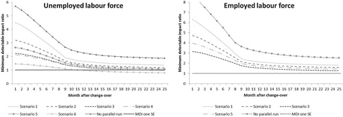
Figure 3 shows the MDI ratios of the different scenarios in relation to different periods after the changeover for the unemployed and the employed. For the unemployed, a sixth scenario was added to illustrate the effect of the times-series model if it is applied after the full parallel run of 100%–100% for a period of 18 months. The MDI ratio for the scenario without a parallel-run converged to a value of approximately 2 and 3 for the unemployed and employed labour forces, respectively. Thus, under this scenario, detecting an impact of one SE cannot be achieved. For example, in relation to the unemployed series of Scenario 1, a one SE impact still cannot be achieved with the predefined accuracy criterion after 24 months. Conversely, in relation to Scenario 4, this precision can be obtained after 19 months and in relation Scenario 6, this precision can be obtained after 11 months.

Figure 3. Minimum detectable impact ratio at the 5% significance level and 50% power obtained with the times-series model for different periods after the changeover among the unemployed labour force (left panel) and the employed labour force (right panel).

The results showed that if the results of a relatively small parallel run are improved with a times-series model, the initial estimates of the statistical impact obtained with the parallel run are likely to be revised after, for example, a period of 12 months. The simulation study was also used to estimate the expected amount of revisions between the estimates obtained for the parallel runs under the five scenarios and the times-series model 12 months after finalising the parallel run. As expected, the size of the revisions decreased with the sample size of the parallel run. The expected revision (see the ‘Average’ column of Table 5) is approximately 5.8% under Scenario 1, 4% under Scenario 2 and 2.7% under Scenario 3.

Table 5. The relative SEs for the impact measurement estimates and revisions for the unemployed labour force in percentage points after 12 months under different parallel-run options.

	RG1	RG2	RG3	RG4	RG5	RG6	RG7	RG8	Average
SE of impact
No PR	3.18	3.35	3.45	3.52	3.58	3.63	3.66	3.69	3.5
Scenario 1	2.36	2.47	2.51	2.54	2.57	2.63	2.67	2.74	2.6
Scenario 2	2.05	2.13	2.15	2.17	2.19	2.23	2.29	2.37	2.2
Scenario 3	1.74	1.79	1.79	1.79	1.81	1.84	1.91	2.00	1.8
Scenario 4	1.70	1.75	1.74	1.75	1.77	1.80	1.86	1.95	1.8
Scenario 5	1.88	1.95	1.96	1.97	1.99	2.03	2.09	2.18	2.00
Scenario 6	1.42	1.44	1.43	1.43	1.44	1.47	1.52	1.61	1.47
Revision
Scenario 1	5.62	6.13	5.88	6.53	4.71	5.71	5.54	5.93	5.8
Scenario 2	3.97	4.22	3.93	4.57	3.29	3.89	3.82	4.02	4.0
Scenario 3	2.73	2.83	2.59	3.11	2.23	2.56	2.58	2.65	2.7
Scenario 4	2.60	2.69	2.45	2.95	2.12	2.43	2.45	2.51	2.52
Scenario 5	3.29	3.46	3.17	3.77	2.71	3.15	3.13	3.25	3.24
Scenario 6	1.69	1.72	1.55	1.88	1.38	1.54	1.58	1.56	1.61

Table 6 provides the final SEs and revisions of the SIM estimates for the employed labour force across the different scenarios in terms of the percent points 12 months after finalising the parallel run.

Table 6. The relative SEs for the impact measurement estimates and revisions for the employed labour force in percentage points after 12 months under different parallel-run options.

	RG1	RG2	RG3	RG4	RG5	RG6	RG7	RG8	Average
SE of impact
No PR	0.57	0.58	0.58	0.61	0.64	0.63	0.63	0.65	0.61
Scenario 1	0.37	0.36	0.35	0.36	0.38	0.37	0.37	0.40	0.37
Scenario 2	0.31	0.30	0.29	0.30	0.31	0.31	0.31	0.33	0.31
Scenario 3	0.25	0.23	0.22	0.22	0.23	0.23	0.24	0.26	0.27
Scenario 4	0.25	0.23	0.22	0.22	0.23	0.23	0.24	0.26	0.27
Scenario 5	0.27	0.28	0.28	0.29	0.29	0.30	0.31	0.33	0.29
Revision
Scenario 1	0.77	0.87	0.81	0.90	0.67	0.78	0.78	0.83	0.80
Scenario 2	0.58	0.63	0.59	0.67	0.50	0.57	0.57	0.61	0.59
Scenario 3	0.38	0.41	0.37	0.44	0.32	0.36	0.36	0.37	0.38
Scenario 4	0.38	0.41	0.37	0.44	0.32	0.36	0.36	0.37	0.38
Scenario 5	0.48	0.52	0.48	0.56	0.41	0.47	0.47	0.49	0.49

Revisions were calculated as the mean over the absolute value of the difference between the initial estimate of the parallel run and the times-series estimate 12 months after finalising the parallel run. A comparison of the size of the revisions to the SE of the SIM shows that the revisions were still substantial, particularly in cases of small parallel runs. As expected, the size of the revision decreased as the size of the parallel run increased. As illustrated with Scenario 6 in relation to the unemployed labour force, the times-series model still produced revisions after a full parallel run designed to observe a SIM of one SE at a 5% significance level and a power level of 50%.

4.3. Revision analysis for the hybrid option

The purpose of this analysis is to understand the properties of the hybrid option. This option uses the initial estimates of statistical impacts (in Figure 4, ini SE has been shown in light grey) from a small parallel run, which may not be as accurate as desired, as inputs to a times-series model (SSM) to improve the accuracy 12 months after finalising the parallel run. Specifically, we sought to explore the relationships between the SEs of the initial estimates (ini SE), the SEs of the final statistical impacts (SE 12 months after changeover) and revision size 12 months after the changeover.

Figure 4. Comparisons of the initial SE from parallel run, final SE and revision after the 12-month changeover.

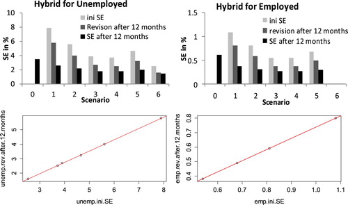
It appears that the regression lines fit the simulated results very well in relation to both employed and unemployed labour forces. Table 7 shows regression results and performance. Both the coefficients of the ini SE for the unemployed and employed were 0.78. This suggests that the hybrid option reduces approximately 80% of errors regardless of the quality of the ini SE.

Table 7. Revision size regressing on ini SE.

	Unemployed	Employed
Intercept	–0.367054 (0.021980)	–0.0395645 (0.0008405)
ini SE	0.779785 (0.004307)	0.7774410 (0.0010967)
Null deviance	10.9734000	1.2628e-01
Residual deviance	0.0016739	1.0051e-06
R^2	0.99984	0.999992

Table 8 shows the results of regressing the SE of the final estimates from the hybrid option 12 months after the changeover onto the initial SE (ini SE) from the parallel run. The coefficients of ini SE for the unemployed and employed series were 0.21 and 0.18, respectively. This suggests that the hybrid option still retains approximately 20% of the errors in the final estimates after the 12-month changeover regardless of the quality of ini SE.

Table 8. SE of final estimates regressing on ini SE.

	Unemployed	Employed
Intercept	0.99578 (0.05123)	0.169087 (0.009134)
ini SE	0.20939 (0.01004)	0.180600 (0.011918)
Null deviance	0.8002000	0.0069333
Residual deviance	0.0090932	0.0001187
R^2	0.988636	0.98288

As Tables 7 and 8 show, the results were consistent across both the unemployed and employed labour forces. The ini SE figures were not exactly equal to the Revision plus SE of final estimates; however, it can confidently be concluded from the coefficients of ini SE that the hybrid option reduces the errors by 80% over the 12 months after the changeover regardless of the quality of the ini SEs. Some errors (approximately 20%) are still likely to remain in the final estimates.

5. Discussion and future research

This paper presented a set of SSM models and evaluations for a range of options that measured the statistical impacts of a survey redesign. In this study, the ABS LFS redesign was used as a case study. The paper showed that by modelling the differences of the GREG estimates for the control and treatment groups at the rotation group level, the model for measuring statistical impact from a parallel run simplified the conventional SSM intervention analysis. This proposed model should be more robust than the conventional SSM intervention approach against rapid real-world changes. Additionally, as there is no need to model the ‘true’ population, the proposed model has a number of advantages over the conventional SSM intervention approach. Notably, the proposed model:

• Eliminates possible complications related to modelling the ‘true’ population during parallel-run periods;

• Avoids the smoothing effect because of the lagged composite weights;

• Takes account of the dynamics of the sample rotation induced process more effectively; and

• Exact (rather than diffuses) initialision of the Kalman filter with a-priori information, as the model is stationary and the expected variances (covariances) of the states are used to speed up the Kalman filter convergence rate.

Theoretical deliberation and the empirical simulation study provided us with an understanding of the relationship between the precision of detecting a statistical impact and:

1. the parallel-run parameters (i.e., the intra-cluster correlation between the treatment and control groups, the sample size and the duration of the parallel run);

2. the effect of sampling errors (i.e., the correlation structure of statistical impacts at the rotation group level and how it affects the statistical impact on the final composite estimate); and

3. the improvement and revision properties of the hybrid option after the changeover.

The information presented in this paper shows how the survey parallel parameters, the characteristics of the LFS survey (e.g., intra-cluster correlation and sampling errors) and the properties of the SSM affect the precision of an estimated statistical impact. Insight in the accuracy obtained with the various options are in combination with cost calculations very helpful for the top management to make a dedicated decision between the different strategies to quantify discontinuities.

In relation to the options considered for measuring impact and implementing change, while a scenario without a parallel run is relatively inexpensive, it has major disadvantages in terms of the risks related to the quality of the published times-series data (particularly coherence and interpretability) during the changeover period. In addition, in the absence of a designed experiment, there is no control over the accuracy requirements for the minimum detectable differences. Thus, the required accuracy criterion that a difference of one SE should be detected at a 5% significance level and a power of 50% is unlikely to be achievable with this approach. For a critically important survey such as the LFS, a large-scale parallel run is required (assuming a low appetite for accepting statistical impacts on the time series).

There are two possible ways to reduce the costs of a parallel run. Either the precision goal that an impact of one SE must be detectable would have to be relaxed or revisions to the estimated impact would have to be acceptable. In the latter case, the times-series modelling approach could be combined with a smaller sample size for the parallel run (as illustrated by the six different scenarios investigated in Section 4).

However, it should be noted that in relation to small parallel runs, there is a large risk that the revision of the initial estimates for the SIM is substantial, as the small parallel run does not produce precise initial estimates. This suggests that the decision to make the changeover would be based on an imprecise initial estimate. In a worst case scenario, the initial SIM estimates might suggest a small impact but the final SIM estimates could be substantially larger 12 months after the changeover. Notably, this risk would decline by increasing the size of the parallel run and could be visualised by looking at the ratio of the revision and the SE of the final SIM estimates (see Figure 3).

Our study of the hybrid option suggests that useful information obtained from the SIM in Phase 1 activities, such as small experiments, field tests and dress rehearsals, could be used as priors for the SSM of a parallel run. Thus, using the SSM modelling approach, the SIM information obtained from a current phase could be used as the priors and input to the SSM of the next phase via an exact initialisation of the states of the level breaks in the Kalman filter. The SIM precision could also be continually improved over the three phases.

We conclude that the hybrid option is the preferred method for statistical impact measurement. This is because this approach uses all available information obtained from the parallel run, the information from the time series observed under the old design before the parallel run and the time series observed under the new design after finalising the parallel run. The method has the flexibility to find the best trade-off between additional costs and increased risk by simulating with which accuracy a statistical impact can be assessed under parallel runs of different length and size.

Further research is required to build on the findings of this study. Some areas for future research include:

• The use of other data sources: The SSM model (Equations 1–5) used for the hybrid option could be extended to include related data sources in a multivariate SUTSE model to improve SIM precision by better predicting the true population. For example, Zhang and Honchar (2016) used unemployment benefit claimant counts (CC) is such a related series for LFS unemployment, and the ANZ job advertisement (ANZadv) and the Department of Employment Internet Job Vacancy index (DoEIVI) are too.

• An alternate SSM formulation: Further study needs to be undertaken to explore alternative SSM model formulations to use the historical data to better improve the Kalman filter convergence rate for shortening parallel-run periods and to reduce the SE of the estimated statistical impact.

Acknowledgements

The authors would especially like to thank the unknown referees and the Associate Editor for careful reading of the manuscript and providing constructive comments as well as Oksana Honchar and Cedric Wong for their valuable contributions to this study, and Sybille McKeown, Professor James Brown, Kristen Stone, Annette Kelly, Rosalynn Mathews, Bruce Fraser, Jacqui Jones and Bjorn Jarvis for their constructive and valuable suggestions and comments. It should be noted that the views expressed in the paper do not necessarily represent those of the ABS and Statistics Netherlands. Any errors in this paper those of the authors.

Disclosure statement

No potential conflict of interest was reported by the authors.

Additional information

Notes on contributors

Xichuan (Mark) Zhang

Dr. Xichuan (Mark) Zhang is a statistical methodology specialist in the areas of time series analysis, econometric and survey methodology at Methodology Division of Australian Bureau of Statistics.

Jan A. van den Brakel

Dr. Jan A. van den Brakel is an extraordinary professor of survey methodology at Maastricht University and works as senior statistician at the Methodology Department of Statistics Netherlands.

Siu-Ming Tam

Dr. Siu-Ming Tam is the former chief methodologist and general manager of Methodology Division of Australian Bureau of Statistics, and honorary professorial fellow of University of Wollongong.

Notes

1 There is anecdotal evidence that Wave 7 contained is less biases and more stable among the eight waves.

2 There was no official accuracy criterion at the time at which the paper was written. A hypothetical accuracy criterion was used purely to assist discussion in this paper.

3 In the context of this paper, population refers to employed or unemployed persons.

4 Further elaboration of this simple model may be needed if evidence emerges that this assumption needs revision (see our discussion of future avenues of research in Section 5).

5 It should be noted that the sampling error for the treatment sample may be larger due to the smaller sample size of the treatment sample.

6 Without losing generality, the state equation is written as an AR(2) process but Waves 1 and 2 follow a white noise process and an AR1 process, respectively.

7 The estimated SE of ${\alpha }_i$ for each replicate appeared to be consistent regardless of the waves and the size of ${\alpha }_i$. avg.se was calculated as the average of all replicates across the eight waves; that is, $avg.se=\text{(}1/8\times 100\text{)}{\sum }_{i=1}^8{\sum }_{j=1}^{100}{\hat{\sigma }}_{i,j}$ where ${\hat{\sigma }}_{i,j}$ is the estimated SE of ${\alpha }_i$ (Wave i) for replicate j.

8 A scientific adjustment is described as a hybrid option in Section 4.2.

9 Most of the precision discussions in this section focused on the rotation group level, as the SE of a statistical impact to the overall composite estimates can be approximated as the SE at the rotation level times a multiplier.

Appendix: Simulated data generation

Data generation description

The observations from the simulated data set followed the following structure, ${\hat{y}}_{i,t}^g=y_t+b_i^g+e_{i,t}^g$and $e_{i,t}^g={\phi }_1{e}_{i-1,t-1}^g+{\phi }_2{e}_{i-2,t-2}^g+{\delta }_{i,t}^g{\delta }_{i,t}^g\sim NID(0,{\sigma }_{\delta }^2)$Note: The above equations are referenced from equation 1, 3–5

where,

$i\in (1,2,\dots ,8)$ is the wave index

$g\in (1,2)$ is the group index where 1 = control group and 2 = treatment group

t is the time period

$y_t$ is the ‘true’ population estimate used in the simulation for employment and unemployment at time t

$b_i^g$ is the rotation group bias (RGB) for the ith wave of the control and treatment group, note that the rotation group bias is time-invariant

$e_{i,t}^g$ is the sampling error for the ith wave of the control and treatment group at time t. It follows an autoregressive process of order 2, AR(2) with the disturbance term ${\mu }_{i,t}^g$,which is normally and independently distributed.

‘True’ population estimate $y_t$

It was estimated by using state space models on the LFS national level estimate. The final estimate was obtained by excluding the standard error component in the state space model.

The rotation group bias $b_i^g$

Each wave had a predefined rotation group bias value subject to a specific employment and unemployment simulation scenario.

AR(2) sampling error $e_{i,t}^g$

For the purposes of this simulation study, $e_{i,t}^g$ and ${\delta }_{i,t}^g$ were required to satisfy a predefined variance covariance structure subject to a specific employment and unemployment simulation scenario.

In order to achieve this, the variance covariance of the AR(2) sampling error disturbance term $Cov\left(e_{i,t}^g\right)$, we generated bivariate time series, $({\delta }_{i,t}^1,{\delta }_{i,t}^2{)}^{\mathrm{\prime }}$ with covariance matrix $Cov\left({\delta }_{i,t}^g\right)$ ($1\le i\le 8$) to reflect the rotation panel design using a standard Gaussian white noise generator.

$e_{i,t}^g$ could then be generated by calculating ${\phi }_1{e}_{i-1,t-1}^g+{\phi }_2{e}_{i-2,t-2}^g+{\delta }_{i,t}^g$ in a cyclical way ($1\le i\le 8$) described below:

Sampling error for wave i = 1 and $mod(t,8)=1$, control and treatment group,

Table

$e_{i,t}^g={\delta }_{i,t}^g$

No AR process

Sampling error for wave i = 2 and $mod(t,8)=1$, control and treatment group,

Table

$e_{i,t}^g={\phi }_1{e}_{i-1,t-1}^g+{\delta }_{i,t}^g$

AR(1) process

Sampling error for wave $3\le i\le 8$ and $3\le mod(t,8)\le 8$, control and treatment group,

Table

$e_{i,t}^g={\phi }_1{e}_{i-1,t-1}^g+{\phi }_2{e}_{i-2,t-2}^g+{\delta }_{i,t}^g$

AR(2) process

Table A1 presents the some key parameters for both control and treatment samples.

Table A1. Parameters for Simulation data generation

	Employed	Unemployed
Sample size per month	30,000
Sampling error AR1 for wave 2	0.835	0.589
Sampling error AR2 for wave 3–8	0.585, 0.3	0.466, 0.208
	RGB Control
RSE at RGB	0.94%	6.60%
b1	0.007	0.058267930
b2	0.001	0.019303798
b3	−0.0044	0.006714512
b4	−0.0044	0.000405143
b5	0.0005	0.017966054
b6	0.0001	0.019514134
b7	0	0
b8	0.0002	0.046400917
	RGB Treatment
b1 + α1	0.6	0.7
b2 + α2	0.001	0.2
b3 + α3	−0.001	0.2
b4 + α4	−0.001	−0.02
b5 + α5	0.001	−0.02
b6 + α6	0	−0.02
b7 + α7	0	0
b8 + α8	−0.6	−0.68

The following pseudo code illustrates the data simulation process

Table

Set RSE RG control sample

Iterate replicates 1–100

Iterate parallel run duration: 11, 13, 15 19

Iterate Kappa: 0.3. 0.5. 0.8, 1

Derived Treatment sample RSE from Kappa.

Iterate intra cluster correlation: 0, 0.3, 0.5, 0.8

Generate both control and treatment sample

End

End

End

End

Note: The simulation programme required the input parameters, ${\phi }_1$ for wave 2, ${\phi }_1$ and ${\phi }_2$ for wave 3 to wave 8, standard error of control and treatment group (reflects $\kappa$), $\rho$, and RGB control and treatment parameters.

In the data simulation, the AR(1) parameter ${\phi }_1$ for wave 2 was different to the AR(1) parameter ${\phi }_1$

A different seed was used to generate the white noise component in each replication and therefore, the simulated observations differed only in the sampling error component.

References

- Aoki, M. (1987). State space modelling of time series. Heidelberg, Berlin: Springer-Verlag.
- Australian Bureau of Statistics (ABS). (2016). Labour force, Australia, April 2016. (ABS Category Number 6202.0). Canberra, ACT: ABS. Retrieved from http://www.abs.gov.au/AUSSTATS/[email protected]/Lookup/6202.0Explanatory%20Notes1Apr%202016?OpenDocument.
- Bell, P. (2001). Comparison of alternative labour force survey estimators. Survey Methodology, 27(2), 53–63.
- Durbin, J., & Koopman, S. J. (2012). Time series analysis by state space methods. Oxford: Oxford University.
- Glass, G. V., Willson, V. L., & Gottman, J. M. (2008). Design and analysis of time-series experiments. Charlotte, NC: Information Age.
- Harvey, A. (1989). Forecasting, structural time series models and the Kalman filter. Cambridge: Cambridge University Press.
- Koopman, S. J., Shephard, N., & Doornik, J. A. (2008). Ssfpack 3.0 statistical algorithms for models in state space form. London: Timberlake Consultants Ltd.
- Pfeffermann, D. (1991). Estimation and seasonal adjustment of population means using data from repeated surveys. Journal of Business and Economic Statistics, 9(2), 163–175.
- Pfeffermann, D., Feder, M., & Singnorelli, D. (1998). Estimation of autocorrecations of survey errors with application to trend estimation in small areas. Journal of Business and Economic Statistics, 16, 339–348.
- Van den Brakel, J. A. (2008). Design-based analysis of embedded experiments with applications in the Dutch labour force survey. Journal of the Royal Statistical Society, Series A, 171(3), 581–613. doi: 10.1111/j.1467-985X.2008.00532.x
- Van den Brakel, J. A., Griffiths, G., Surzhina, T., Wise, P., Blanchard, J., Zhang, X., & Honchar, O. (2017). A framework for measuring the impact of transitions in official statistics. Australian Bureau of Statistics, Research paper 1351.0.55.158, Canberra, Australia.
- Van den Brakel, J. A., & Krieg, S. (2015). Dealing with small sample sizes, rotation group bias and discontinuities in a rotating panel design. Survey Methodology, 41(2), 267–296.
- Van den Brakel, J. A., & Roels, J. (2010). Intervention analysis with state-space models to estimate discontinuities due to a survey redesign. Annals of Applied Statistics, 4(2), 1105–1138. doi: 10.1214/09-AOAS305
- Van den Brakel, J. A., Smith, P. A., & Compton, S. (2008). Quality procedures for survey transitions, experiments, time series and discontinuities. Journal for Survey Research Methods, 2(3), 123–141.
- Van den Brakel, J. A., Zhang, X. (Mark), & Tam, S.-M. (2019). Measuring discontinuities in time series obtained with repeated sample surveys. International Statistical Review, forthcoming.
- Zhang, X., & Honchar, O. (2016). Predicting survey estimates by state space models using multiple data sources. (ABS Category Number 1351.0.55.159). Retrieved from http://www.abs.gov.au/AUSSTATS/[email protected]/DetailsPage/1351.0.55.159August%202017.
- Zhang, X., Van den Brakel, J. A., Honchar, O., Wong, C., & Griffiths, G. (2017). Using state space models for statistical impact measurement of survey redesigns. (ABS Category Number 1351.0.55.160). Retrieved from http://www.abs.gov.au/AUSSTATS/[email protected]/DetailsPage/1351.0.55.160October%20201.