Model-based small area estimation with no samples within the areas, by benchmarking to marginal cross-sectional and time-series estimates

ABSTRACT

Official monthly U.S. labour force estimation at the sub-State level (mostly counties) is based on what is known as the ‘Handbook’ (HB) method, one of the earliest uses of administrative data for small area estimation. The administrative data, however, are poor in coverage and have conceptual deficiencies. Past attempts to correct for the resulting bias of the HB estimates by informal (implicit) modelling have not been successful, due to the absence of regular direct monthly survey estimates at the sub-State level. Benchmarking the sub-State HB estimates each month to the State model dependent estimates helps to correct for an overall bias, but not in individual areas. In this article we propose benchmarking additionally to the annual model-dependent area estimates. The annual models include known administrative data as covariates, and are used to define corresponding monthly sub-State models, which in turn enable producing monthly synthetic estimates as possible substitutes for the HB estimates in real time production. Variance estimates, which account for sampling errors and the errors of the model dependent estimators are developed. Data for sub-State areas in the State of Arizona are used for illustration. Although the methodology developed in this article stems from a particular (but very important) application, it is general and applicable to other similar problems.

KEYWORDS:

• Benchmarking
• Denton method
• mixed models
• variance estimation

1. Introduction

The Bureau of Labor Statistics (BLS) in the U.S.A. produces each month local area employment and unemployment estimates at the sub-State level, known as the Handbook (HB) estimates, formally developed in 1960 (U.S. Bureau of Labor Statistics, 1960; U.S. Bureau of Labor Statistics, Handbook of Methods, 2019). There are over 4,000 sub-State areas in the 50 States of the U.S.A. for which monthly labour force estimates are produced. No monthly survey estimates are available for most of these areas due to high cost of data collection. The American Community Survey (ACS) collects data for the sub-States on a monthly basis, but it is designed to produce annual, rather than monthly estimates.

The monthly HB estimates depend heavily on local area administrative data, obtained from the Unemployment Insurance (UI) system. The data contains current monthly counts of the number of workers receiving UI benefits at the sub-State level, and local monthly payroll employment data from business establishments, with a reporting delay of 4–6 months. Conceptual differences and incomplete coverage prevent the use of the administrative data as adequate substitutes for a proper survey. In fact, except for the decennial census long form data, no direct labour force survey data were collected for the purpose of producing estimates at the local level, until the advent of the American Community Survey (ACS). In an attempt to correct for the deficiencies in the administrative data, the HB method uses implicit models that combine national, regional and State relationships through a series of synthetic methods and special adjustments. (U.S. Bureau of Labor Statistics, 1960; U.S. Bureau of Labor Statistics, Handbook of Methods, 2019). However, large biases remain because of the lack of regular monthly survey information at the appropriate level of geography (county level in most cases).

Unlike at the sub-State area level, monthly State estimates are produced each month by the BLS, based on the Current Population Survey (CPS), conducted by the U.S. Census Bureau. The CPS is a nationwide household survey, collecting data on the labour force characteristics of the civilian noninstitutionalized population, 16 years of age and over. An important feature of the CPS is the 4-8-4 rotating panel design by which households are interviewed for 4 successive months, are dropped from the sample for the next 8 months and then they are interviewed again for 4 additional months. This rotation pattern induces high correlations between the monthly direct estimators even at long lags. To meet national (and State) reliability criteria, about 60,000 housing units are drawn from 824 CPS sample areas. The reliability criterion at the national level is a coefficient of variation no greater than 1.9 percent, assuming an unemployment rate of 6% for the national monthly estimates of the unemployment rate. The reliability criterion for allocating samples to each State is a coefficient of variation no greater than 8% for annual State estimates of unemployment level, assuming an unemployment rate of 6%.

For large (national) samples, the direct survey estimators are used as the official estimates. However, the direct monthly survey estimates of unemployment are not considered reliable at the State level. (There is no explicit reliability criterion for employment.) Consequently, in order to reduce the sampling errors at the State level, time series models have been developed, independently for each State. The models consist of two components: a model for the signal, which is the sum of a stochastic trend, seasonal effects and irregular variations, and a model for the CPS sampling error, with the covariance matrix estimated externally from the individual survey responses. In order to protect (robustify) against sudden national shocks, the State models are combined into a multivariate model with monthly benchmark constraints which force each month the sum of the State model-based estimates of the signal to equal the national CPS direct estimate. Estimators of the variances of the benchmarked estimators that account for all sources of errors have also been developed and are published along with the monthly estimates. (Pfeffermann & Tiller, 2006).

To partly deal with the bias of the monthly sub-State HB estimates, and to ensure consistency with the State model-based estimates, the sub-State HB estimates are ratio adjusted each month to the corresponding model-based State estimate. The resulting adjusted estimates define what is known as the official Local Area Unemployment Statistics (LAUS) estimates. As commented above, the monthly benchmarking reduces the overall bias of the monthly HB estimators in a given State, but it is not effective in eliminating the bias of the estimators for any given local area as illustrated in the empirical results in Section 6.

Starting in 2005, the ACS provides direct annual labour force estimates at the sub-State level of interest. The ACS is the largest, timely and most geographic detailed household survey in the U.S. It collects data on labour force status and other socioeconomic, demographic and housing characteristics in over 4,000 counties or county equivalents, as well as for minor civil divisions, with an overall sampling fraction of 2.5%. Each year a survey questionnaire is mailed out to 3.5 million addresses, with each address sampled for one month during the year, and not considered again for sampling until five years later. Annual estimates are published for areas with at least 20,000 persons. For smaller areas, only five-year moving period estimates are currently published. The annual series are available 9 months after data collection. The 5-year moving period estimates become available after 12 months.

In this article, we develop a methodology that allows estimation of monthly labour force characteristics at the sub-State level, by combining information from three separate sources: Administrative data known monthly at the area level, the annual survey estimates at the area level based on the ACS, and the monthly State-wide estimates based on the CPS. The general idea is to model the annual ACS estimates as functions of the known administrative data, develop monthly models for each area, which are consistent with the annual model, produce synthetic monthly estimates for each area from the monthly models and then obtain final monthly sub-State estimates by two-way benchmarking of the monthly synthetic estimates to the annual model-based ACS estimates and to the monthly model-based CPS estimates. Ratio adjusting the monthly synthetic estimates to the monthly CPS estimates, as a substitute to the HB/LAUS method, produces estimates close to the final benchmarked estimators even during the current year, before the annual ACS data are available. Appropriate variance estimates, which account for the main sources of error are developed. Data for sub-State areas in the State of Arizona are used for illustration.

Section 2 presents the two-way benchmarking of the monthly local area estimates to known cross-sectional and time-series benchmarks. A procedure for preserving the monthly movements in the original monthly series being benchmarked is discussed and applied. Section 3 discusses issues with the use of the direct ACS estimates for benchmarking. These issues are addressed in Section 4 by modelling the annual estimates. In Section 5 we develop the monthly models and use them for producing synthetic monthly sub-State estimates, which are benchmarked to the model-based CPS and ACS estimates. Section 6 illustrates the application of the proposed procedure using data from the State of Arizona. In Section 7 we consider variance estimation. We conclude with a short summary and discussion of remaining work in Section 8, followed by four technical Appendices.

In what follows we refer for convenience to the CPS and ACS estimates as benchmarks for the local sub-State estimates, but as already mentioned in the abstract, the procedure is applicable to other small area estimation problems where no sample data are available at the area level.

2. Benchmarking local area monthly estimates to the ACS and CPS aggregates

2.1. Benchmarking procedure

Table 1 describes schematically the two-way benchmarking in a given year, for areas $c=1,\dots ,C$ of a given State S, where the two benchmarks are (1)- the monthly CPS State estimates (column totals) and (2)- the annual ACS area estimates (row totals).

Table 1. Benchmarked monthly area estimates $w_{c,m}$. ${\mathit{S}}_{\mathit{m}}=\text{monthly}$ CPS State estimates, ${\mathit{A}}_{\mathit{c}}=\text{annual}$ ACS area estimates.

	Months				Year (y)
Areas(c)	1	2	…	12	ACS totals
1	$w_{1,1}$	$w_{1,2}$	…	$w_{1,12}$	$A_1$
$⋮$	$⋮$	$⋮$	$⋮$	$⋮$	$⋮$
C	$w_{C,1}$	$w_{C,2}$	…	$w_{C,12}$	$A_C$
CPS totals	$S_1$	$S_2$	…	$S_{12}$

$\sum _{c=1}^C{w}_{c,m}=S_m,m=1,\dots ,12,\sum _{m=1}^{12}{w}_{c,m}=A_c,c=1,\dots ,C$.

The two-way benchmarking system can be formulated, similar to the calibration procedure of Deville and Särndal (1992) as follows. Denote by n_c,m the true (unknown) count (estimand) in area c at month m, and by d_c,m any initial monthly estimate (say, the HB estimate). The benchmarking consists of finding new estimates, ${\hat{n}}_{c,m}=w_{c,m}$, which are as close as possible to the initial estimates, subject to satisfying the constrains, (1) $\begin{array}{rl}\sum _{c=1}^C{w}_{c,m}& =S_m,m=1,\dots ,12,\\ \sum _{m=1}^{12}{w}_{c,m}& =A_c,c=1,\dots ,C,\end{array}$(1) where ‘as close as possible’ is defined by minimising, (2) $D(d,w)=\sum _{c=1}^C\sum _{m=1}^{12}{(w_{c,m}-d_{c,m})}^2/d_{c,m}.$(2) (More than one year can be considered simultaneously. Below we also consider the case of moving 5-year benchmarks.)

Remark 2.1:

The use of this distance function provides explicit expressions for the benchmarked estimates {$w_{c,m}$}. See Appendix 1. Other distance functions can be used but the resulting estimates do not necessarily have explicit expressions, which can be important for subsequent analysis like variance estimation.

DISCUSSION. When proposing a new statistical estimation procedure, it is common to justify its use by considering theoretical properties such as bias, consistency, optimality, etc. Can we claim any of these properties under our proposed approach? The answer is largely negative. To begin with, Pfeffermann and Barnard (1991) proved that even with the availability of unbiased estimators at the small area level, and with known model hyper-parameters, there exist no uniformly best linear unbiased predictor (BLUP) (for every area), satisfying random benchmark constraints. Isaki, Tsay, and Fuller (2000) commented that by application of benchmarking with random benchmarks, some of the benchmarked small area predictors will be better than the not benchmarked predictors, but other will be worse. In our case the situation is even worse, as no unbiased sub-State estimators exist.

Are our benchmarked predictors unbiased? The state-space models for the monthly CPS predictors have been tested and found to fit the data well, see e.g. Tiller (1992) and Pfeffermann and Tiller (2006). In Sections 4 and 6 we provide some diagnostics validating the generalised linear mixed model (GLM) we fit to the annual ACS estimates. Thus, both of these models can be assumed to provide empirical BLUP (EBLUP) of the benchmarks (with estimated hyper-parameters). In Section 5 we propose the use of initial sub-State model-based predictors and in Appendix 1 we obtain the explicit expression of the final benchmarked predictors as a function of the three sets of predictors. Consequently, and as stated more rigorously in Lemma A1 in Appendix 1, if the model assumed for the true sub-State means is correct, then the benchmarked predictors are approximately unbiased and consistent for the true means but as noted above, they are generally not ‘best’ for every area. The situation is clearly different with non-random benchmarks, since in this case the benchmarks provide new information about the area means.

Benchmarking to known margins, whether random or fixed, is not new and goes back to Iterative Proportional Fitting proposed by Deming and Stephan (1940). Purcell and Kish (1980) propose the use of what is known as Structure Preserving Estimation (SPREE), later extended by Zhang and Chambers (2004) to Generalised SPREE (GSPREE). All these methods assume reliable cell estimates (sub-States in our case) and attempt to preserve interactions, measured in terms of ratios of counts, observed for these estimates (either exactly or proportionally). See Rao and Molina (2015, Chapter 3) for discussion of these and other related methods, with illustrations. In a recent article, Dostal, Gabler, Ganninger, and Münnich (2016) likewise use the Chi-square distance function in (2) subject to two-way constraints as in (1), for enhancing the German census estimates in small domains. Their set-up differs from ours in some key elements:

1. The margins $\left\{S_m\right\}$ and $\left\{A_c\right\}$ are considered as fixed known values, whereas in our case they are random, model-based estimators,

2. Their initial cell estimates $\left\{d_{c,m}\right\}$ are sample estimators obtained from a sample drawn by a proper sampling design, whereas in our case no sample estimates are available for the sub-State areas,

3. The authors propose variance estimators which only partly account for the variances of their sample estimators.

As already stated, no reliable sub-State estimates are available and our benchmarks are random, obtained from models fitted to the marginal sample estimates. Our approach provides explicit benchmarked estimates and as discussed below and shown in Appendix 2, it generalises to the case where only 5-year moving totals are available, a situation not considered in the literature other than in Sverchkov and Tiller (2016). For the case of annual ACS totals, we propose in Section 7 and Appendix 4 a bootstrap procedure for estimating the variance of the final benchmarked predictors.

2.2. The case of moving 5-year benchmarks

Next consider the case of small sub-States for which only moving 5-year ACS estimates are available. Denote by $n_{cym}$ the true (unknown) count in area c at month m of year y, and by $d_{cym}$ the corresponding initial estimate. The benchmarking consists in this case of finding new estimates, ${\hat{n}}_{cym}=w_{cym}$, minimising, (3) $\begin{array}{rl}D(d,w)& =\sum _{y=1}^Y\sum _{c=1}^C\sum _{m=1}^{12}{\left(w_{cym}-d_{cym}\right)}^2/d_{cym},\text{s.t.}\\ \sum _{c=1}^C{w}_{cym}& =S_{ym},m=1,\dots ,12;y=1,\dots ,\text{Y};\\ \sum _{y=k+1}^{y=k+5}\sum _{m=1}^{12}{w}_{cym}& =A_{c,y}^{y+5},k=0,\dots ,\mathrm{Y}-\text{5; }\\ c& =1,\dots ,C.\end{array}$(3) In this formulation, S_ym denotes the State total in month m of year y, $A_{c,y}^{y+5}=\sum _{j=1}^5{A}_{c,y+j},y=0,1,\dots ,(Y-5)$ are the five year totals, and $Y$ defines the last year.

See Appendix 2 for derivation of the benchmarked estimators obtained in this case.

Remark 2.2:

Large and small sub-States can be combined in a single benchmarking exercise, see Sverchkov and Tiller (2016), but our empirical estimates obtained this way are not satisfactory and we need to study this option further. A possible explanation is that as shown by Nagaraja and McElroy (2015), five years ACS total estimates are not the sum of one-year estimates. In particular, the five-year samples are drawn differently from the one-year samples. Hereafter we focus on benchmarking the monthly sub-State area estimates in areas with single year ACS estimates, plus an artificially constructed balance-of-State area with an annual ACS estimate, defined as the difference between the State ACS estimate and the sum of the annual estimates for areas with single year estimates.

Remark 2.3:

Since the benchmarking for any given year is independent of other years, one can benchmark each year separately which is simpler computationally than benchmarking all the years simultaneously. This is not true with moving five-year totals.

2.3. Denton corrections

A potential problem with the application of the procedure described so far is the possibility of producing breaks in the series, when large year-to-year changes occur in the annual ACS estimates. A possible solution to this problem is to use a benchmarking approach designed to preserve movements in the original time series. Denton (1971) proposed minimising the magnitude of such distortions when benchmarking a single time series by minimising the sum of squares of the monthly changes in the proportional differences to the initial estimates, that is; (4) $\begin{array}{rl}& \text{Minimize}{D}_{den}\left(w,d\right)\\ & =\sum _{t=2}^T{\left[\frac{(w_{c,t}-d_{c,t})}{d_{c,t}}-\frac{(w_{c,t-1}-d_{c,t-1})}{d_{c,t-1}}\right]}^2,\\ & \text{s}\text{.t}.\sum _{m=1}^{12}{w}_{c,m}=A_c,c=1,\dots ,C.\end{array}$(4) Since the Denton method does not necessarily satisfy the State monthly constraints, we first apply the method to the initial estimates in each area separately, and then benchmark the Denton adjusted series by application of the two-way benchmarking procedure described before, satisfying simultaneously the monthly CPS and annual ACS constraints. This approach tends to preserve relative monthly movements in the initial estimates. Bikker, Daalmans, and Mushkudiani (2013) use a combination of Chi-square distance and Denton distance simultaneously.

3. Issues in relying on (Direct) ACS estimates for benchmarking

There are a number of issues (concerns) in using the direct ACS estimates for benchmarking: conceptual and measurement differences compared to the CPS, lower reliability, long delays in publication, and missing values. In what follows we discuss these issues in some detail.

While the employment and unemployment definitions in the ACS and CPS are similar, there are differences in the way the two surveys are designed and conducted, which may generate differences in the estimated values: mode of data collection (Mail and Internet $\to \mathrm{C}\mathrm{A}\mathrm{T}\mathrm{I}\to \mathrm{C}\mathrm{A}\mathrm{P}\mathrm{I}$ at ACS, CAPI and CATI at CPS, where CATI and CAPI define, respectively, Computer Assisted Telephone Interview and Computer Assisted Personal Interview); reference week (week prior to the date of filling out the questionnaire in the ACS, week including the 12th of the month in the CPS) and response rates (much higher in CPS). Additionally, the CPS uses the 4-8-4 rotation scheme described in the Introduction, with 1st and 5th time interviews carried out by CAPI and the other interviews conducted by CATI, while the households sampled for the ACS are included in the sample only once.

Figure 1 indicates non-negligible differences between the ACS and CPS estimates at the national level. The ACS unemployment rates tend to be significantly higher than the CPS rates (with the exception of 2008–2009). On the other hand, the ACS employment counts are significantly lower than the CPS counts until 2008. Since 2008, the ACS employment counts are much closer to the CPS counts, following a change in the questionnaire, designed to improve the measurement of employment status. The change enabled the ACS to capture more employed persons, particularly those with irregular work arrangements (Kromer & Howard, 2011). However, the change in questionnaire did not reduce the overestimation of the unemployment rates compared to the CPS rates.

Figure 1. Annual ACS & CPS estimates, 2002–2016.

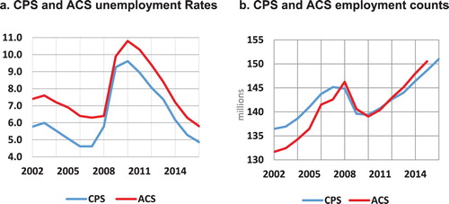
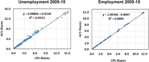
While there are clear differences between the CPS and ACS estimates (especially for unemployment), the ACS and CPS shares of the various States out of the corresponding national totals are surprisingly close. This is seen in Figure 2, where the annual ACS State shares of the ACS national totals are regressed against the annual CPS State shares of the CPS national totals. (Similar results hold for major metropolitan areas as shares of their respective State totals.)

Figure 2. Annual ACS (y) and CPS(x) State shares of annual national totals.

To reconcile the ACS estimates with the model-based State CPS estimates in our benchmarking process, we modify the annual ACS sub-State estimates so that their sum equals the annual CPS State model estimate. This is accomplished by computing adjusted annual ACS sub-State estimates, obtained by multiplying the areas’ share of the annual total State ACS by the annual model-based State CPS; (5) ${\tilde{A}}_{cy}=\frac{A_{cy}}{\sum _{c=1}^C{A}_{cy}}\times S_y,y=1,2,\dots ,Y;$(5) ${\tilde{A}}_{cy}$ is the adjusted annual ACS estimate for an area c in a given year y within a State, and $S_y=\sum _{m=1}^{12}{S}_{my}$ is the annual total of the monthly State CPS model estimates.

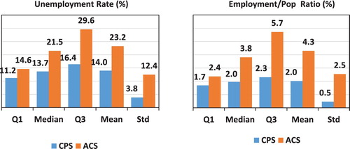
A second major issue is the relatively low reliability of the ACS estimates at the sub-State level. Even though the ACS sample is of substantial size (2.5% sampling rate, with oversampling in small areas), there are nonetheless major reliability problems. Figure 3 compares the direct monthly CPS coefficients of variation (CVs), with the annual ACS CVs, separately for employment and unemployment. The monthly CPS estimates are not considered to be sufficiently reliable for direct use as official statistics. Since the ACS CVs are even higher, their direct use is highly problematic. Large variation in area population sizes lead to large variation in sample sizes and hence large differences in reliability of the estimates.

Figure 3. Monthly State CPS CVs (before modelling) and annual ACS CVs, 2005–2016.

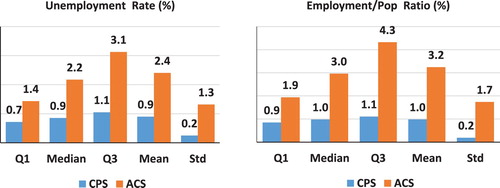
The reliability of the annual changes in the ACS is even worse than the reliability of the level estimates. Unlike the CPS where 75% of the households are retained in the sample from month-to-month and 50% from year-to-year, an entirely new sample of ACS households is drawn each year, which basically doubles the variance of a change estimate compared to the variance of a level estimate. Figure 4 shows that the ACS annual changes are much less reliable than the changes in the monthly direct CPS estimates.

Figure 4. Standard errors of change in monthly CPS and annual ACS, 2005–2016.

A third problem with the annual ACS estimators is that they are not available for a current year, thus preventing benchmarking the monthly estimates in real time. The annual ACS estimates are released only 9 months after data collection due to processing requirements.

Finally, there is a practical problem of dealing with missing values. It happens occasionally that areas which have been eligible for publication of annual estimates drop in size below the 20,000 mark, in which case the annual estimates are no longer published. Also, data may be suppressed due to special circumstances, (confidentiality, data quality, table suppression,). In order to benchmark all the area estimates in a consistent manner, it is necessary to impute the missing values before benchmarking.

For all the above reasons, it is imperative to model the adjusted annual ACS estimates. Section 4 details the model specification.

4. Enhancing the utility of ACS by modelling the annual estimates

We fit a generalised linear mixed (GLM) model to produce better quality estimates for annual ACS, using the annual ACS estimates as the dependent variable and data from two main sources of area specific information, currently used in the LAUS programme as known regressors: UI- unemployment insurance claims, and QCEW- the Quarterly Census of Earnings and Wages (annual average of monthly counts of persons on payroll). For a total of C areas and Y years, we fitted the following cross-sectional – time series mixed model: (6) $\begin{array}{rl}{r}_{cy}& =R_{cy}+e_{cy}=(\alpha +{\alpha }_c)+x_{cy}(\text{β}+{\text{β}}_c)+e_{cy};\\ c& =1,\dots ,C,y=1,\dots ,Y,\end{array}$(6) where $R_{cy}$ is the (unknown) true ratio of employment (unemployment) to the population aged 16+ in area c at year y, $r_{cy}$ is the sample (ACS) estimate, $e_{cy}=(r_{cy}-R_{cy})$ is the sampling error, independent across time and areas with ‘known’ variances ${\sigma }_{cy}^2$ (estimated externally), $x_{cy}$ represents the known regressor; ($x_{cy}=U{I}_{cy}/Po{p}_{cy}$ for the unemployment model, $x_{cy}=QCE{W}_{cy}/Po{p}_{cy}$ for the employment model, with $Po{p}_{cy}$ denoting the population size), $\alpha ,\text{β}$ are fixed intercept and slope parameters and ${\alpha }_c,{\text{β}}_c$ are random area intercept and slope. The model assumes normality of the error terms; $e_{cy}\sim N(0,{\sigma }_{cy}^2),{\alpha }_c\sim N(0,V_{\alpha }),{\text{β}}_c\sim N(0,V_{\text{β}})$.

In the empirical results of Section 6, we fit the model using SAS Proc Mixed, with Restricted Maximum Likelihood (REML) option for estimating the model parameters, and Empirical Best Linear Unbiased Prediction (EBLUP) to predict the random intercepts, (random effects in small area estimation terminology). The computations require matrices of high dimension. An alternative approach is based on a state-space representation, which provides an efficient recursive approach for likelihood calculation and estimation. Appendix 3 describes this approach and presents results of applying it to data from Arizona. As expected and illustrated in Appendix 3, the use of the two approaches yields the same predictions.

Remark 4.1:

In the empirical study we tried adding fixed and random time effects to the model, but it did not improve the goodness of fit in any significant way for the series considered.

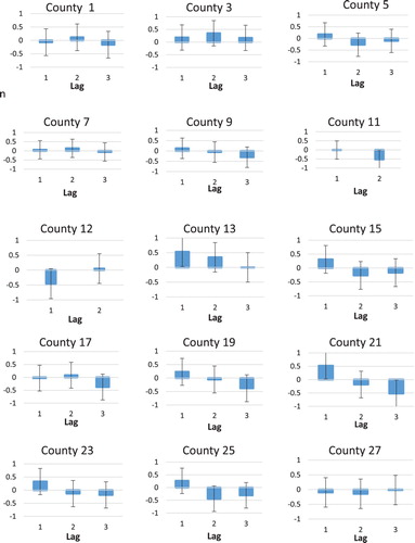
An examination of the correlograms for each of the 15 time series for the mixed model residuals in the 15 counties of ARIZONA (see Section 6 for more details), shows no evidence of large autocorrelations except in a few cases, providing further evidence for the goodness of fit of the model. (The autocorrelations refer to the estimated residuals based on a small number of annual estimates). Figure 5 shows the estimated autocorrelations along with approximate 95% confidence intervals. The number of annual estimates ranged from 12 for areas with no missing data during the observation period 2005–2016, to 9 estimates for areas with missing data. The number of lags computed is equal to one fourth of the number of observations per area.

Figure 5. Autocorrelations of model residuals with approximate 95% confidence intervals.

For benchmarking, we convert the predicted ratios ${\hat{r}}_{cy}$ under the model to levels; ${\hat{L}}_{cy}={\hat{r}}_{cy}\times Po{p}_{cy}$, and ratio adjust the levels to the State annual controls, producing model based annual ACS benchmarks (controls), $\begin{array}{rl}{\tilde{A}}_{cy}& =\frac{{\hat{L}}_{cy}}{\sum _{c=1}^C{\hat{L}}_{cy}}\times S_y,y=1,2,\dots ,Y,\\ c& =1,\dots ,C,\text{see}\text{Equation}\text{(5)}.\end{array}$

5. Synthetic predictors for monthly data

As pointed out in Section 3, a major problem with the use of the annual ACS estimates is that they are released only 9 months after data collection due to processing requirements. In particular, no ACS benchmarks are available for a current year. While this problem can be resolved by imputing the missing ACS estimates under the model, another related problem is that no HB or LAUS estimates are available to initialise the benchmarking before the end of a current year.

In order to deal with this problem, we propose to produce synthetic monthly predictors from a model that is consistent with the annual ACS model defined in Section 4. For this, we first seasonally adjust (SA) the monthly covariates and then use the annual model and parameter estimates to generate the monthly (ratio) estimates, (7) $\begin{array}{rl}{\hat{r}}_{cym}& =(\hat{\alpha }+{\hat{\alpha }}_c)+SA(x{)}_{cym}(\widehat{\text{β}}+{\widehat{\text{β}}}_c);\\ c& =1,\dots ,C;m=1,\dots ,12;\text{y}=1,\dots ,Y.\end{array}$(7) We seasonally adjust the covariates because the models for the annual ACS estimates (employment and unemployment) use annual versions of the covariates, which are free of seasonal effects. We also found in our empirical study that when using the original (seasonal) covariates, the model can generate unrealistically large fluctuations, as happens with the unemployment models where the slope coefficients are greater than one. As before, the resulting monthly ratio estimates are converted to levels, which are then ratio adjusted to the monthly State controls, before applying the Denton adjustment and the two-way benchmarking (See Remark 5.2 below.)

Remark 5.1:

In practice, we use the initial synthetic predictors for all the years and not just for the last current year, because the use of the synthetic predictors yields much better final predictors than when initialling the process with the HB or LAUS estimates, in the sense of minimising the extent of revision when ACS controls become available. See the empirical results in Section 6.

Remark 5.2:

By ratio adjusting the monthly synthetic sub-State estimates, which by our model are not seasonal, to the monthly State estimates, which are seasonal, part of the State seasonality is added to the sub-State estimates, but it does not imply the same seasonal pattern for each of the sub-States. For example, although not shown in the article, the seasonality featuring in Figure 8 for the Yuma county is much weaker than the seasonality of the monthly State control.

Remark 5.3:

It may be argued that the model holding for the annual ACS estimates does not define uniquely the models holding for the monthly sub-States. This is true in principle, known as the ecological fallacy, but in the absence of reliable monthly estimates at the sub-State level, this is the best we can do. On the other hand, and as already stated in Section 2.1, if the model assumed for the sub-States is correct (as far as a model is ever ‘correct’), the final two-way benchmarked predictors are approximately unbiased and consistent. See Appendix 1.

Remark 5.4:

One could ask why we don’t use the monthly State CPS model for each of the sub-State areas, as an alternative procedure to obtain synthetic monthly estimates. Notice, however, that the CPS State models account for the complex rotation pattern of the CPS samples described in the Introduction, whereas the monthly ACS samples are independent cross-sectionally and over time, so that they obey a very different model. Moreover, the State model does not contain the geographically detailed information in the ACS data (the area covariates) which is critical for reducing the model bias. See Section 6 for illustration.

6. Empirical illustrations- State of Arizona

In this section we apply our estimation procedure to the 15 counties comprising the State of Arizona. Table 2 contains information for this State for the years 2005–2016.

Table 2. Information about counties (sub-States) in the State of Arizona.

Total number of counties	15
Counties of size 20k ≤ Pop < 65k	6
Counties of size Pop ≥ 65k	9
Number of missing ACS estimates	14

We start by presenting in Table 3 the model hyper-parameter estimates as obtained when fitting the model (6) by application of SAS Proc Mixed procedure, using restricted maximum likelihood (REML) for estimating the fixed model parameters, and empirical best linear unbiased prediction (EBLUP) for predicting the random effects. The procedure enables inputting the externally estimated ACS variances for each year.

Table 3. Model (6) parameter estimates, Arizona.

Coefficients, Unemployment/Pop16+				Coefficients, Employment/Pop16+
Coefficient	Estimate	t-value	Pr> |t|	Coefficient	Estimate	t-value	Pr> |t|
Intercept	0.02255	8.97	<.0001	Intercept	0.3300	8.74	<.0001
UI/Pop	2.5354	9.92	<.0001	QCEW/Pop	0.4451	4.32	<.0001
*Yr10	9.3 × 10^−3	15.16	<.0001	*Yr10	0.02979	1.96	<.0001
Variances, Unemployment/Pop				Variances, Employment/Pop
Variance	Estimate	z-value	Pr >| z|	Variance	Estimate	z-value	Pr > |z|
Intercept	5.5 × 10^−5	1.60	0.0549	Intercept	0.01105	1.32	0.0929
UI/Pop	0.6135	1.91	0.0282	QCEW/Pop	0.08421	1.27	0.1026

*Yr10 is a dummy variable controlling for the introduction of new ACS estimates in 2010.

Figure 6 shows the Conditional Pearson Residuals (CPR), defined as the difference between the observed dependent variable and the predicted value, divided by the square root of the corresponding ACS variance. The Figure contains four panels: 1- plot of the CPR against the predicted values, 2- histogram of the CPR, with the normal density overlaid, 3- Q-Q plot of the CPR, 4- summary results.

Figure 6. Diagnostics based on Conditional Pearson Residuals (CPR).

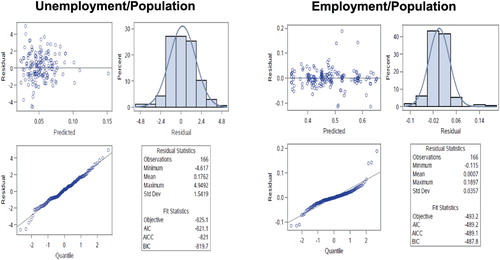
The residuals are fairly well behaved. The plots show some long tails at both ends of the data distribution, suggesting the presence of outliers.

Next we focus on Yuma County, located on the southwestern corner of Arizona, bordering Mexico. There has been considerable public questioning of Yuma’s HB and LAUS monthly unemployment figures, which appear unusually high (up to 30%, highest in the nation), even though its population has grown continuously by 20% (Bare, 2012). As a border community there are large flows of workers from across the border which raises the possibility that many UI claimants may reside in Mexico or even California, but counted as Yuma residents. As we now show, by benchmarking to the ACS annual estimates, we succeed in eliminating or at least reducing very significantly the apparent bias of the HB and LAUS estimates.

Figure 7 compares the annual unemployment LAUS rates, the ACS rates ratio adjusted to the annual model-based State controls (Ratio adjusted ACS), and the model-based ACS rates (Model-Based ACS). The LAUS annual rates are as high as 25% in some years, compared to a high of about 13% for the ACS.

Figure 7. Annual unemployment rates for Yuma where the ACS estimates and the model-based ACS predictions are adjusted to the annual model-based CPS.

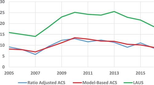
The LAUS annual rates in Figure 7 are as high as 25% in some years, compared to a high of about 13% for the ACS.

Figures 8 and 9 illustrate our benchmarking process. Figure 8 shows for Yuma county the HB estimates, the LAUS estimates obtained by ratio adjusting the HB estimates to the monthly State, model-based CPS estimates (the State controls), the LAUS estimates after benchmarking to the model-based ACS estimates using the Denton method to preserve the proportional monthly change in the series (DLAUS), and the final estimates obtained by applying the two-way benchmarking process to the DLAUS series (BMK DLAUS). The DLAUS and BMK DLAUS for the YUMA series are seen to be virtually equal, suggesting that after applying the Denton adjustment to the LAUS estimates, both the monthly and the annual constraints are practically satisfied for this county, with no need for further adjustments by the two-way benchmarking process.

Figure 8. Unemployment rate estimates for Yuma County as obtained by HB, LAUS, Denton LAUS (DLAUS) and benchmarked Denton LAUS (BMK DLAUS). 2005–2016.

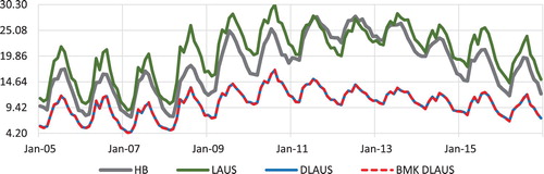
Figure 9. Unemployment Rate estimates for Yuma county: Synthetic, Dsynthetic, BMK Dsynthetic and BMK DLAUS. 2005–2016.

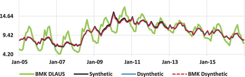
Figure 9 compares the synthetic unemployment rates with the Denton adjusted synthetic series (Dsynthetic), the two-way benchmarked Denton adjusted synthetic series (BMK Dsynthetic) and the BMK DLAUS series (same as in Figure 8). It is interesting to note that the three series – synthetic (generated from the model), Dsynthetic and BMK Dsynthetic are virtually indistinguishable. In other words, the synthetic estimates are, by construction, very close to the final benchmarked estimates. On the other hand, the synthetic estimates are far less seasonal than the BMK DLAUS estimates since the covariates are seasonally adjusted. Benchmarking the HB series to the monthly State model-based CPS estimates to produce the LAUS series, sometimes introduces weak seasonal variation. When the series are all seasonally adjusted (not shown), the resulting series are very close to each other.

Finally, Table 4 indicates that the findings for Yuma extend to the other counties in Arizona. The table shows how much the input (initial) series has to be changed in magnitude on average, over all the months and across all the counties, to satisfy both the annual and the monthly constraints. We consider two alternative annual constraints: the (ratio adjusted) ACS controls and the model-based ACS controls.

Table 4. Average absolute percent change between input series and benchmarked estimates. Arizona, all counties. 2005–2016.

	Unemployment		Employment
Input Series	ACS Controls	Model-based ACS Controls	ACS Controls	Model-based ACS Controls
HB	44.05%	34.60%	8.97%	7.42%
DHB	4.58%	4.57%	0.90%	0.90%
LAUS	26.39%	16.92%	7.44%	5.68%
DLAUS	0.79%	0.76%	0.01%	0.01%
SYNTH	19.06%	0.31%	4.47%	0.08%
DSYNTH	0.05%	0.01%	0.00%	0.00%

The use of HB requires by far the largest revisions. The LAUS is second, while initialising with the synthetic model estimates and applying the Denton corrections virtually requires no further benchmarking. Initialising with the Denton corrected LAUS estimates also yields very satisfactory results, as explained by the fact that these estimates are first ratio adjusted to satisfy the monthly State controls and then adjusted to satisfy the annual controls. Notice also that the size of the revisions is uniformly reduced when replacing the ratio adjusted ACS estimates by the model-based ACS controls.

7. Variance estimation

In Appendix 4 we develop a parametric bootstrap (BS) procedure for estimating the variance of the two-way benchmarked predictors, as obtained when initialising the estimation process with the synthetic predictors defined in Equation (7). As discussed before and illustrated in the empirical study in Section 6, initialising the estimation process with the synthetic estimators yields much better final sub-State estimates, compared to the final estimates obtained when initialising the benchmarking with the HB or the LAUS estimates. In fact, since no variances can be computed for the HB or the LAUS estimates unless when conditioning on the wrong HB estimates, no variances can be developed for the final sub-State predictors when initialising the estimation process with the HB or LAUS estimates.

In Table 5 we compare the BS variance estimators with the corresponding model-based estimators of the variances of synthetic predictors, as produced by Proc mixed in SAS. We are interested in 3 types of estimates:

Table 5. Model and Bootstrap (BS) Standard Errors (SE), and Coefficients of Variation (CV) for Arizona Unemployment by county, averaged over all monthly values. 10,000 Bootstrap samples. 2005–2016.

		SE BS					CV BS
Column/County	SE Model ${\hat{L}}_{cym}$	${\hat{L}}_{cym}$	${\hat{L}}_{cym}^{\ast }$	${\hat{L}}_{cym}^{\ast \ast }$	Synthetic, Columns (2/3)	CV Model ${\hat{L}}_{cym}$	${\hat{L}}_{cym}$	${\hat{L}}_{cym}^{\ast }$	${\hat{L}}_{cym}^{\ast \ast }$
1	2	3	4	5	6	7	8	9	10
1	217	197	264	264	1.10	0.07	0.06	0.10	0.10
3	419	381	442	443	1.10	0.09	0.08	0.10	0.10
5	451	411	500	499	1.10	0.08	0.07	0.10	0.10
7	182	165	193	194	1.10	0.08	0.08	0.10	0.10
9	120	119	119	120	1.01	0.11	0.11	0.12	0.12
11	32	31	32	32	1.04	0.11	0.10	0.12	0.12
12	76	68	77	78	1.11	0.09	0.08	0.11	0.11
13	12,691	11,919	8,195	8,198	1.06	0.10	0.10	0.08	0.08
15	704	651	815	816	1.08	0.08	0.07	0.10	0.10
17	344	313	423	422	1.10	0.07	0.06	0.10	0.10
19	3,269	3,019	3,477	3,478	1.08	0.08	0.07	0.09	0.09
21	1,152	1,120	1,404	1,404	1.03	0.07	0.07	0.10	0.10
23	146	154	166	166	0.95	0.09	0.09	0.12	0.12
25	753	742	924	923	1.02	0.07	0.07	0.10	0.10
27	649	629	1,255	1,254	1.03	0.04	0.04	0.09	0.09

Estimators: ${\hat{L}}_{cym}={\hat{R}}_{cym}^{b}Po{p}_{cym},{\hat{L}}_{cym}^{\ast }=\text{ratio}$ adjusted ${\hat{L}}_{cym},{\hat{L}}_{cym}^{\ast \ast }=\text{Calibrated}$ ${\hat{L}}_{cym}^{\ast }$

Model Standard Error =$Po{p}_{cym}\sqrt{Var\left({\hat{R}}_{cym}^b\right)}$ (computed for every BS sample); $Var\left({\hat{R}}_{cym}^b\right)=Var\left({\hat{\alpha }}_c^{\ast b}\right)+S{A}^2\left(x_{cym}\right)Var\left({\widehat{\text{β}}}_c^{\ast b}\right)+2SA\left(x_{cym}\right)Cov\left({\hat{\alpha }}_c^{\ast b},{\widehat{\text{β}}}_c^{\ast b}\right);$ ${\hat{\alpha }}_c^{\ast b}=\left({\hat{\alpha }}^b+{\hat{\alpha }}_c^b\right),{\widehat{\text{β}}}_c^{\ast b}=\left({\widehat{\text{β}}}^b+{\widehat{\text{β}}}_c^b\right)$.

Bootstrap (BS) Standard Errors:

BS ${\hat{L}}_{cym}=\sqrt{\left(1/B\right)\sum _{b=1}^B{\left({\hat{L}}_{cym}^b-{\overline{\hat{L}}}_{cym}^b\right)}^2}$, BS ${\hat{L}}_{cym}^{\ast }$= $\sqrt{\left(1/B\right)\sum _{b=1}^B{\left({\hat{L}}_{cym}^{\ast b}-{\overline{\hat{L}}}_{cym}^{\ast b}\right)}^2}$, BS ${\hat{L}}_{cym}^{\ast \ast }=\sqrt{\left(1/B\right)\sum _{b=1}^B{\left({\hat{L}}_{cym}^{\ast \ast b}-{\overline{\hat{L}}}_{cym}^{\ast \ast b}\right)}^2}$. See Appendix 4 for more details.

${\hat{L}}_{cym}-$Model estimate of the signal converted to level, ${\hat{L}}_{cym}={\hat{R}}_{cym}\ast Po{p}_{cym}$; ${\hat{R}}_{cym}$ is the synthetic predictor (Equation (7)), $Po{p}_{cym}$ is the population size for sub-State area c at month m of year y.

${\hat{L}}_{cym}^{\ast }-$ Ratio adjusted ${\hat{L}}_{cym}$ to monthly State controls $\left(S_{my}\right)$, ${\hat{L}}_{cym}^{\ast }=\left({\hat{L}}_{cym}/\sum _c{\hat{L}}_{cym}\right)\ast S_{my}$,

${\hat{L}}_{cym}^{\ast \ast }-$Benchmarked ${\hat{L}}_{cym}^{\ast }$ to monthly and annual controls.

The Table contains the model-based and BS standard errors (SE), and Coefficients of Variation (CV) for each of the 15 counties in Arizona, using 10,000 bootstrap replications. See Appendix 4 for details. The figures in the table are averages over all simulated monthly values.

When comparing the average SEs and CVs of the synthetic estimators, the model SEs and CVs in columns 2 and 7 tend to be a bit higher, but generally close to the corresponding bootstrap estimates in columns 3 and 8. (The CVs are virtually the same.)

The picture is different when comparing the model-based SEs and CVs of the synthetic estimators (columns 2 and 7), to the BS SE’s and CVs of the benchmarked estimators in columns 4, 5 and 9, 10 respectively. As can be seen, except for County 13 with the very extreme SEs, the BS SEs are larger, and occasionally considerably larger than the corresponding model-based and BS SE’s of the synthetic estimators. This outcome is easily explained by the fact that the sub-State benchmarked estimators depend also on the random benchmarks, which adds to the variances of the benchmarked estimators. On the other hand, there is basically no difference between the SEs of the predictor ${\hat{L}}_{cym}^{\ast },$ which only ratio adjusts to the monthly CPS predictor, and the corresponding SEs of the final predictor $,{\hat{L}}_{cym}^{\ast \ast }$, based on the two-way benchmarking. This latter result provides additional support to the use of the synthetic model during a current year when calibration to the annual ACS estimates is not (yet) possible.

Remark 7.1:

The results in Table 5 raise, what looks a priori like a legitimate question, of why one should benchmark the synthetic predictors, given that the benchmarked predictors have larger SEs than the synthetic predictors. Recall, however, that the monthly synthetic predictors are the result of a model that matches the annual ACS model, with no way to ascertain its correctness, having no samples at the sub-State level. Benchmarking increases the variance of the final monthly predictors, but it guaranties that they agree with the reliable annual ACS predictors and more so, with the reliable monthly CPS predictors. As discussed in Section 2, benchmarking to random benchmarks generally increases the variances of the benchmarked predictors.

Remark 7.2:

The BS procedure potentially accounts for all sources of variance, but it is much more computationally intensive, which could be an issue, given that we aim to produce variance estimates for all the U.S. sub-State areas simultaneously, in real time. Development of a linearization-based procedure for variance estimation that similarly accounts for all (or at least the most important) variance components is tempting, but it seems formidable to account properly for all the covariances involved, which cannot be ignored. Recall that the two-way benchmarked predictors are functions of three sets of predictors, obtained from two different surveys, with the synthetic estimators being generated from the ACS model such that for each county their annual sum is close to the corresponding ACS annual total.

8. Conclusions and further work

The monthly ratio adjusted LAUS estimates and the synthetic model-based estimates have similar levels and hence, both reduce the bias of the HB estimates in current use by about the same magnitude. The big difference between the two series is in the size of the revisions from the not benchmarked to the benchmarked series. The revisions required for the synthetic estimates are much smaller.

The monthly synthetic model estimates provide a natural way to produce real time estimates when annual ACS benchmarks for the current year are not available. Benchmarking the LAUS estimates is an ex-post operation that would require some kind of additional work such as forecasting the annual ACS benchmarks for the current year. Benchmarking the monthly series with the model based ACS controls produces much smoother monthly series and reduces the size of the benchmarked revisions, compared to the original (not-modeled) ACS controls.

Our next major task is to apply our proposed procedure to the small counties for which only moving five year ACS estimates are available (Section 2.2 and Appendix 2). One of the problems with the moving five year estimates is that while the annual ACS sampling errors are independent over time, the 5-year sampling errors are highly autocorrelated by construction. Sampling error variances for 5 period estimates are available but not the autocovariances. Another problem is how to obtain monthly synthetic estimators from the model fitted to the moving five year estimates. A possible way to deal with this problem is to fit an annual state-space model to the 5-year ACS estimates, which will allow prediction of the annual estimates, and then proceed as with the larger sub-State areas.

Remark 8.1:

There is a possibility that we shall obtain single year estimates for the small counties in the near future, in which case we may not need to benchmark the estimates for these counties separately.

Disclosure statement

No potential conflict of interest was reported by the authors.

Additional information

Notes on contributors

Danny Pfeffermann

Danny Pfeffermann is the National Statistician and Head of the Central Bureau of Statistics of Israel. He is a Professor of Statistics at the Hebrew University of Jerusalem, Israel, and at the University of Southampton, UK. His main research areas are analytic inference from complex sample surveys, small area estimation, seasonal adjustment and trend estimation, non-ignorable nonresponse and more recently, mode effects and proxy surveys. He is the recipient of several prestigious awards, most recently the Julius Shiskin Award. When receiving this award, he gave a lecture which forms the basis for the present paper.

Michael Sverchkov

Michael Sverchkov is a Research Mathematical Statistician at the U.S. Bureau of Labor Statistics, Washington DC. His main research areas are analytic inference from complex sample surveys and in particular, informative samples with non-ignorable nonresponse, small area estimation and seasonal adjustment.

Richard Tiller

Richard Tiller is a Mathematical Statistician at the U.S. Bureau of Labor Statistics, Washington DC. His main research areas are small area estimation, with emphasis on problems related to modelling continuous survey series with complex sampling error correlation structure and strong seasonality. He also works on issues in seasonal adjustment.

Lizhi Liu

Lizhi Liu is a Mathematical Statistician at the U.S. Bureau of Labor Statistics, Washington DC. She works on developing statistical software for small area estimation research, as well as maintaining and improving Local Area Unemployment Statistics (LAUS). She also works on issues in seasonal adjustment.

Appendices

Appendix 1. Benchmarking of Initial estimates to State and Annual estimates

In what follows we consider a single year and hence we drop the subscript y (defining the year) from the notation. (As mentioned before, we apply the two-way benchmarking for the large sub-States for every year separately. See Appendix 2 for the two-way benchmarking in the case of the small sub-States.) For consistency with Appendix 4 on variance estimation, we consider the case where we initialise the benchmarking with the synthetic estimators ${\hat{R}}_{cm},c=1,\dots C$ (areas), $m=1,\dots ,M$ ($M=12$, months) defined by (7), but the same procedure applies to any other set of initial estimates and other dimensions of the two-way table. See also Table 1 in Section 2. Similarly to Section 4, we convert the ratios ${\hat{R}}_{cm}$ to levels; ${\hat{L}}_{cm}={\hat{R}}_{cm}\times Po{p}_{cm}$ ($Po{p}_{cm}$ is the population size). Denote by $L_{cm}$ the true value in cell (c,m), which under the model (7) equals, $L_{cm}=\left[\right(\alpha +{\alpha }_c)+SA(x{)}_{cm}(\text{β}+{\text{β}}_c\left)\right]Po{p}_{cm}$. Denote by $T_1,\dots ,T_C$ the true row totals ($A_1,,,A_C$ in the notation of Table 1), and by $T_{C+1},\dots ,T_{C+M}$ the true column totals ($S_1,\dots ,S_M$ in the notation of Table 1. In our application $M=12$.) Define $\mathbf{\text{T}}=(T_1,\dots ,T_C,T_{C+1},\dots ,T_{C+M}{)}^{\mathrm{\prime }}$ (a column vector).

For every cell $(c,m)$, define the column vector ${\mathbf{\text{x}}}_{cm}=(x_{cm1},\dots ,x_{cm(C+M)}{)}^{\mathrm{\prime }}$, where $x_{cmi}=1$ if $i=c$ or $i=C+m$, and 0 otherwise, such that ${\mathbf{\text{x}}}_{cm}=(\underset{c-1}{\underbrace{0,\dots ,0}},1,\underset{C-c}{\underbrace{0,\dots ,0}},\underset{m-1}{\underbrace{0,\dots ,0}},1,\underset{M-m}{\underbrace{0,\dots ,0}}{)}^{\mathrm{\prime }}$. With $\left\{L_{cm}\right\}$ defining the true area totals, it follows that $\sum _{c=1}^C\sum _{m=1}^M{L}_{cm}{\mathbf{\text{x}}}_{cm}=\mathbf{\text{T}}$ (the true marginal totals).

We wish to benchmark the synthetic estimates ${\hat{L}}_{cm}$ to the model-based ACS and CPS totals, $\widehat{\mathbf{\text{T}}}=({\hat{T}}_1,\dots ,{\hat{T}}_C,{\hat{T}}_{C+1},\dots ,{\hat{T}}_{C+M}{)}^{\mathrm{\prime }}$. Following Deville and Särndal (1992), the benchmarked predictors $\left\{w_{cm}\right\}$ under the loss function (2) are: (A1) $\begin{array}{rl}{w}_{cm}& ={\hat{L}}_{cm}(1+{\mathbf{\text{x}}}_{cm}^{\mathrm{\prime }}\lambda );\lambda ={\left[\sum _{c=1}^C\sum _{m=1}^M{\hat{L}}_{cm}{\mathbf{\text{x}}}_{cm}{{\mathbf{\text{x}}}^{\mathrm{\prime }}}_{cm}\right]}^{-1}\\ & \times (\widehat{\mathbf{\text{T}}}-\sum _{c=1}^C\sum _{m=1}^M{\hat{L}}_{cm}{\mathbf{\text{x}}}_{cm}).\end{array}$(A1)

Remark A1:

The model-based ACS and CPS estimates, $\widehat{\mathbf{\text{T}}}=({\hat{T}}_1,\dots ,{\hat{T}}_C,{\hat{T}}_{C+1},\dots ,{\hat{T}}_{C+M}{)}^{\mathrm{\prime }}$ are not the same as $\sum _{c=1}^C\sum _{m=1}^M{\hat{L}}_{cm}{\mathbf{\text{x}}}_{cm}$, as they are obtained from the models fitted to the observed ACS and CPS totals, without use of the initial estimates.

Remark A2:

Deville and Särndal (1992) consider modification of the base sampling weights in survey sampling estimation, such that sample estimators of totals of variables that use the modified weights equal known totals of these variables, known as ‘calibration’. Here we use their algorithm for modification of the available (initial) estimates, known as ‘benchmarking’.

For possible problems with the inversion of the matrix $\sum _{c=1}^C\sum _{m=1}^M{\hat{L}}_{cm}{\mathbf{\text{x}}}_{cm}{\mathbf{\text{x}}}_{cm}^{\mathrm{\prime }}$ and how to deal with them, see Deville and Särndal (1992).

Lemma A1:

Under the models used for generating the benchmarks (ACS and CPS totals), and the model used to generate the synthetic predictors $\left\{{\hat{L}}_{cm}\right\}$, the final benchmarked predictor $w_{cm}$ defined by (A1) is approximately unbiased and consistent for all $c=1,\dots ,C;m=1,\dots ,12$, in the sense that ${lim}_{Y\to \mathrm{\infty },C\to \mathrm{\infty }}\left(w_{cm}\right)=L_{cm}$.

Proof

Outline of Proof

By Taylor approximation, the predictor $w_{cm}$ in (A1) can be approximated as, (A2) $\begin{array}{rl}{w}_{cm}& \cong {\hat{L}}_{cm}\left\{1+{\mathbf{\text{x}}}_{cm}^{\mathrm{\prime }}{\left[\sum _{c=1}^C\sum _{m=1}^M{L}_{cm}{\mathbf{\text{x}}}_{cm}{\mathbf{\text{x}}}_{cm}^{\mathrm{\prime }}\right]}^{-1}\right.\\ & \times \left.\left[(\widehat{\mathbf{\text{T}}}-\mathbf{\text{T}})+\left(\sum _{c=1}^C\sum _{m=1}^M(L_{cm}-{\hat{L}}_{cm}){\mathbf{\text{x}}}_{cm}\right]\right.\right\}.\end{array}$(A2)

Suppose first that all the models’ hyper-parameters are known. As $Y\to \mathrm{\infty },C\to \mathrm{\infty }$, $Cov[{\hat{L}}_{cm},(\widehat{\mathbf{\text{T}}}-\mathbf{\text{T}}\left)\right]\cong 0$, $Cov[{\hat{L}}_{cm},(\sum _{c=1}^C\sum _{m=1}^M(L_{cm}-{\hat{L}}_{cm}){\mathbf{\text{x}}}_{cm}]\cong 0$ and hence, by the formula for the expectation of the product of uncorrelated random variables, and the assumptions of the Lemma that $E\left({\hat{L}}_{cm}\right)=L_{cm}$ for all c and m and $E(\widehat{\mathbf{\text{T}}}-\mathbf{\text{T}})=0$, we find that $E\left(w_{cm}\right)=L_{cm}$.

As $Y\to \mathrm{\infty },C\to \mathrm{\infty }$, the estimators of the models’ hyper-parameters converge to the true hyper-parameters, thus completing the proof.

Appendix 2. Benchmarking when only moving five year ACS estimates

In Appendix 1 we consider benchmarking based on annual ACS data. Here we consider the small areas for which only moving five year totals are available for each area. Denote, as before, by $L_{cym}$ the true estimand for area c in year y and month m and by ${\hat{L}}_{cym}$ the corresponding synthetic estimator.

Denote by $T_1,\dots ,T_H=T_1,\dots ,T_{12},T_{13},\dots T_{24},\dots ,T_{(Y-1)12+1},\dots T_{12Y}$ the true monthly State totals for years $y=1,\dots ,Y$, ($H=12Y$), and by $T_{H+1},\dots ,T_{H+J}$ the area annual totals, such that for $j=Y(c-1)+y$, $T_{H+j}$ is the annual total in year y for area c ($J=Y\times C$). Let $\mathbf{\text{T}}=(T_1,\dots ,T_H,T_{H+1},\dots ,T_{H+J}{)}^{\mathrm{\prime }}$. Define for each $(h,j)$, the vector ${\mathbf{\text{x}}}_{hj}=(x_{hj\text{,1}},\dots ,x_{hj,H+J}{)}^{\mathrm{\prime }}$, where $x_{hj,i}=1$ if $i=h$ or $i=H+j$, and $x_{hj,i}=0$ otherwise. ${\mathbf{\text{x}}}_{hj}=(\underset{h-1}{\underbrace{0,\dots ,0}},1,\underset{H-h}{\underbrace{0,\dots ,0}},\underset{j-1}{\underbrace{0,\dots ,0}},1,\underset{J-j}{\underbrace{0,\dots ,0}}{)}^{\mathrm{\prime }}$. Finally, for $h=12(y-1)+m$ and $j=Y(c-1)+y$, denote $n_{hj}=L_{cym}$ and $d_{hj}={\hat{L}}_{cym}$. Then,$\sum _{h=1}^H\sum _{j=1}^J{n}_{hj}{x}_{hj}=\mathbf{\text{T}}$. Notice that for each pair $(h,j)$ corresponds only one set of values $(c,y,m)$.

With these definitions, the estimates $d_{hj},h=1,\dots ,H,j=1,\dots ,J$ can be adjusted to satisfy the known column and row totals similar to (A1): find new estimates $w_{hj},h=1,\dots ,H,j=1,\dots ,J$, minimising the distance function $D(\mathbf{\text{d}},\mathbf{\text{w}})=\sum _{h=1}^H\sum _{j=1}^J{(w_{hj}-d_{hj})}^2/d_{hj}$, satisfying the constraints $\sum _{h=1}^H\sum _{j=1}^J{w}_{hj}{\mathbf{\text{x}}}_{hj}=\mathbf{\text{T}}$. As in (A1), the solution of the minimisation problem is explicit: (A3) $\begin{array}{rl}{w}_{hj}& =d_{hj}(1+{\mathbf{\text{x}}}_{hj}^{\mathrm{\prime }}\lambda );\lambda ={\left[\sum _{h=1}^H\sum _{j=1}^J{d}_{hj}{\mathbf{\text{x}}}_{hj}{\mathbf{\text{x}}}_{hj}^{\mathrm{\prime }}\right]}^{-1}\\ & \times (\mathbf{\text{T}}-\sum _{h=1}^H\sum _{j=1}^J{d}_{hj}{\mathbf{\text{x}}}_{hj})\end{array}$(A3) Next, assume that all the monthly State totals, $T_1,\dots ,T_H$, are known, but only moving 5-year area totals are known: $\begin{array}{rl}& T_{H+1}\left(5\right),T_{H+2}\left(5\right),\dots ,T_{H+Y-4}\left(5\right),T_{H+Y+1}\left(5\right),T_{H+Y+2}\left(5\right),\\ & \dots ,T_{H+2,Y-4}\left(5\right),\dots ,T_{H+J-Y+1}\left(5\right),T_{H+J-Y+2}\left(5\right),\dots ,\\ & T_{H+J}\left(5\right)\end{array}$where $T_t\left(5\right)=T_t+T_{t+1}+\cdots +T_{t+4}$. Let $x_{hjt}\text{(5)}=x_{hjt}+\cdots +x_{hjt+\text{4}}$ and define, ${\mathbf{\text{T}}}^{\mathbf{\ast }}=[T_1,\dots ,T_H,T_{H+1}(5),T_{H+2}(5),\dots ,T_{H+Y-4}(5),T_{H+Y+1}(5),T_{H+Y+2}(5),\dots ,T_{H+2Y-4}(5),\dots ,$ $T_{H+J-Y+1}\left(5\right),$ $T_{H+J-Y+2}\left(5\right),\dots ,T_{H+J}\left(5\right){]}^{\mathrm{\prime }}$, and ${\mathbf{\text{x}}}_{hj}^{\ast }=[x_{hj\text{1}},\dots ,x_{hjH},x_{hjH+\text{1}}\text{(5)},x_{hjH+\text{2}}\text{(5)},\dots ,x_{hjH+Y-\text{4}}\text{(5)},x_{hjH+Y+\text{1}}(5),x_{hjH+Y+\text{2}}(5),x_{hjH+\text{2}Y-4}(5),\dots ,x_{hjH+J-Y+\text{1}}(5),x_{hjH+J-Y+\text{2}}(5),x_{hjH+J-\text{4}}(5){]}^{\mathrm{\prime }}$.

We again have $\sum _{h=1}^H\sum _{j=1}^J{n}_{hj}{\mathbf{\text{x}}}_{hj}^{\ast }={\mathbf{\text{T}}}^{\ast }$ and therefore the estimates $d_{hj},h=\text{1},\dots ,H,j=\text{1},\dots ,J$ can be adjusted by benchmarking as, (A4) $\begin{array}{rl}{w}_{hj}& =d_{hj}(1+\mathbf{\text{x}}{}_{hj}^{\ast \mathrm{\prime }}\lambda );\lambda ={\left[\sum _{h=1}^H\sum _{j=1}^J{d}_{hj}{\mathbf{\text{x}}}_{hj}^{\ast }\mathbf{\text{x}}{{}_{hj}^{\ast }}^{\mathrm{\prime }}\right]}^{-1}\\ & \times ({\mathbf{\text{T}}}^{\ast }-\sum _{h=1}^H\sum _{j=1}^J{d}_{hj}{\mathbf{\text{x}}}_{hj}^{\ast })\end{array}$(A4)

Remark A3:

A similar approach can be applied for any combination of moving totals, for example, 1-year totals for some areas and 5-years totals for other areas. Cf. Sverchkov and Tiller (2016).

Appendix 3. State-space representation of the generalised linear mixed model

A state-space representation of our model provides an alternative approach to Proc Mixed for fitting the model defined in Section 4 to the ACS annual estimates. The state-space representation consists of an ‘observation equation’ and a ‘transition equation’ (Harvey, 1989). For Equation (6); $r_{cy}=R_{c,y}+e_{c,y}=({\alpha }_c+\alpha )+x_{c,y}({\text{β}}_c+\text{β})+e_{c,y};c=1,\dots ,C,y=1,\dots ,Y$, the observation equation is given by (A5) $r_{cy}={{\mathbf{\text{h}}}^{\mathrm{\prime }}}_{cy}{\mathbf{\text{z}}}_{cy}+e_{cy};{\mathbf{\text{h}}}_{cy}^{\mathrm{\prime }}=(1,1,x_{cy},x_{cy}),{\mathbf{\text{z}}}_{cy}=[\alpha ,{\alpha }_c,\text{β},{\text{β}}_c{]}^{\mathrm{\prime }}.$(A5) The ‘state vector’, ${\mathbf{\text{z}}}_{cy}$ contains the unknown fixed and random regression coefficients.

The general form of the transition equation is given by (A6) ${\mathbf{\text{z}}}_{cy}={\text{T}}_{cy}{\mathbf{\text{z}}}_{c,y-1}+{\mathbf{\text{v}}}_{cy};E\left({\mathbf{\text{v}}}_{c,y}{{\mathbf{\text{v}}}^{\mathrm{\prime }}}_{c,y}\right)=Q_y$(A6) where ${\mathbf{\text{v}}}_{cy}$ is the vector of the random disturbances in the model. In our case,

For $y=1$, ${\text{T}}_{cy}={\text{T}}_{c1}=Diag\left(1,0,1,0\right);{\text{Q}}_y=Q_1=Diag\left(0,V_{\alpha },0,V_{\text{β}}\right)$,

For $y>1$, ${\text{T}}_{cy}={\text{T}}_c=Diag\left(1,1,1,1\right);{\text{Q}}_{cy}=Q=Diag\left(0,0,0,0\right)$.

To apply the model to all the areas, we combine the data for each sub-State area, sorted by time, to a single vector of all of the observed values. ${\mathbf{\text{r}}}_y=\left(r_{C,y},r_{C-1,y},\dots ,r_{1,y}\right)\text{compare}\text{with}\left(\text{A}5\right)$The observation equation for all the areas may be expressed: (A7) $\mathbf{\text{r}}=\text{H}\mathbf{\text{z}}+\mathbf{\text{e;}}\text{H}=\oplus [{\mathbf{\text{h}}}_{C,y},{\mathbf{\text{h}}}_{C-1,y}\dots ,{\mathbf{\text{h}}}_{1,y}]$(A7) (the notation $\oplus$ is used for ‘block diagonal’), ${\mathbf{\text{z}}}_y=({\mathbf{\text{z}}}_{C,y},{\mathbf{\text{z}}}_{C-1,y},\dots ,{\mathbf{\text{z}}}_{1,y}{)}^{\mathrm{\prime }}$, $\mathbf{\text{e}}=(e_{C,y},e_{C-1,y},e_{1,y}{)}^{\mathrm{\prime }}$.

The corresponding transition equation is now, (A8) $\begin{array}{rl}{\mathbf{\text{z}}}_y& ={\text{T}}_y{\mathbf{\text{z}}}_{y-1}+{\mathbf{\text{v}}}_y,{\text{T}}_y=\oplus [{\text{T}}_{Cy},{\text{T}}_{C-1,y},\dots {\text{T}}_{1,y}],\\ {\mathbf{\text{v}}}_y& =({\mathbf{\text{v}}}_{C,y},{\mathbf{\text{v}}}_{C-1,y},\dots ,{\mathbf{\text{v}}}_{1,y}{)}^{\mathrm{\prime }}.\end{array}$(A8) Given estimates of the model variances, the Kalman filter is used to produce predicted values of $R_{cy}$ and its variance. See Harvey (1989) for details. Before processing the first observation, the state vector and its variances must be initialised. The state vector values are set to zero and the variances of the random intercept and slope are set to their unconditional variances. Improper priors are used to initialise the variances of the fixed intercept and slope. When processing the first observation from another area, the estimates of the random state variables are re-initialised. Once the filtering is complete, the filtered estimates are revised by a smoothing algorithm, which runs back through the data to strengthen the predictions at each time point by using the information from all the available data (Harvey, 1989).

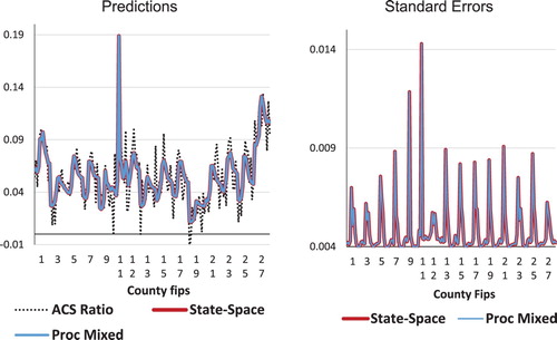
The state-space model has been fitted in SAS Proc IML and applied to the Arizona data. Figure A1 compares the results for the 15 counties in Arizona as obtained by use of the state-space model and by use of the Proc Mixed procedure in SAS (used for the empirical study in Section 6). The ACS Ratios are the predictions of $R_{cy}$ (Equation (6)). On the horizontal axis are labels for each of the counties identified by their Fips (Federal Information Processing Standards) code. As can be seen, the state-space results are virtually identical to Proc Mixed. However, the latter procedure uses an algorithm that requires matrices of dimension that equals the total number of observations ($12\times Y\times C$), which grows larger and larger as more years with data become available. In contrast, with the recursive structure of the Kalman filter and the smoother, the dimensions of the matrices are independent of the number of yearly observations, and they require only the inversion of the prediction error covariance matrix.

Figure A1. Predictions of annual ACS ratios (${\hat{R}}_{cy}$) and standard errors as obtained from state-space modelling and Proc Mixed. 2005–2016.

Appendix 4. Parametric bootstrap procedure for variance estimation

Our proposed parametric BS procedure consists of the following steps, using the index c for county, y for year, m for month and b for bootstrap iteration:

(A) Generate a single set of true values $R_{cy}$ as:

$R_{cy}={\alpha }_c^{\ast }+{\text{β}}_c^{\ast }\ast x_{cy}$, $y=2005-2016,$ c = 1, … , 15.

${\alpha }_c^{\ast }=a+a_c$, $a_c\sim N\left(0,{\sigma }_a^2\right)$, ${\text{β}}_c^{\ast }=\text{β}+{\text{β}}_c$, ${\text{β}}_c\sim N\left(0,{\sigma }_{\text{β}}^2\right).$

$a,\text{β},{\sigma }_a^2,{\sigma }_{\text{β}}^2$ are the estimates obtained when fitting the model (6) to Arizona’s data.

(B) Generate independently B times:

1. State CPS monthly totals from normal distributions with means equal to the empirical predictors ($S_{ym}$) and variances (${\sigma }_{S_{ym}}^2$), as estimated from the State CPS model for Arizona; $T_{ym}^{CPS\left(b\right)}\sim N\left(S_{ym},{\sigma }_{S_{ym}}^2\right),m=1,\dots ,12.$

2. Annual State total of monthly signal predictions: $T_y^{CPS\left(b\right)}=\sum _{m=1}^{12}{T}_{ym}^{CPS\left(b\right)}$.

3. Annual ACS controls:

3a. Generate annual sample labour force to pop ratios: $r_{cy}^b$ $=R_{cy}+e_{cy}^b,$ $e_{cy}^b\sim N\left(0,{\sigma }_{cy}^2\right)$,

where ${\sigma }_{cy}^2$ are the empirical variance estimates from the ACS sample.

3b. Use the estimates $r_{cy}^b$ as input to Proc Mixed to estimate the regression coefficients ${\hat{\alpha }}^b,{\hat{\alpha }}_c^b,{\widehat{\text{β}}}^b,{\widehat{\text{β}}}_c^b$, and variances ${\sigma }_{\alpha }^{b2},{\sigma }_{\text{β}}^{b2}$. Predict new annual ratios ${\hat{R}}_{cy}^b$ and compute variances ${\hat{V}}_{cy}^{b2}=Var\left({\hat{\alpha }}_c^{\ast b}\right)+x_{cy}^{2}Var\left({\widehat{\text{β}}}_c^{\ast b}\right)+2x_{c,y}Cov({\hat{\alpha }}_c^{\ast b},{\widehat{\text{β}}}_c^{\ast b})$, where ${\hat{\alpha }}_c^{\ast b}=\hat{\alpha }+{\hat{\alpha }}_c^b$, ${\widehat{\text{β}}}_c^{\ast b}=\widehat{\text{β}}+{\widehat{\text{β}}}_c^b$.

3c. Convert annual predictions to level, ${\hat{L}}_{cy}^b={\hat{R}}_{cy}^b\times Po{p}_{cy}$, and compute ${\hat{T}}_y^{ACS\left(b\right)}=\sum _{c=1}^n{\hat{L}}_{cy}^b$.

3d. Calculate annual ratio adjusted controls: ${\hat{L}}_{cy}^{\ast b}=\left(\frac{T_y^{CPS\left(b\right)}}{{\hat{T}}_y^{ACS\left(b\right)}}\right){\hat{L}}_{cy}^b$.

4. Compute monthly predictions:

4a. Predict true monthly ratios: ${\hat{R}}_{cym}^b={\hat{\alpha }}_c^{\ast b}+{\widehat{\text{β}}}_c^{\ast b}SA\left(x_{cym}\right)$, where ${\hat{\alpha }}_c^{\ast b}$ and ${\widehat{\text{β}}}_c^{\ast b}$ are from step 3b and $SA\left(x_{cym}\right)$ is the seasonally adjusted monthly covariate.

4b. Convert to level, ${\hat{L}}_{cym}^b={\hat{R}}_{cym}^b\times Po{p}_{cym}$.

4c. Prorate to CPS State model predictions, ${\hat{L}}_{cym}^{\ast b}=\frac{{\hat{L}}_{cym}^b}{\sum _{c=1}^C{\hat{L}}_{cym}^b}\times {\mathrm{T}}_{ym}^{CPS\left(b\right)}$.

4d. Compute benchmarked predictors ${\hat{L}}_{cym}^{\ast \ast b}$, which satisfy both the monthly controls, $T_{ym}^{cps\left(b\right)}$ in 2 and the annual controls, ${\hat{L}}_{cy}^{\ast b}$ in 3d.

(C) Compute Bootstrap standard errors of monthly predictions:

$S{E}_{\hat{T}}^{boot}=\sqrt{\frac{1}{B}\sum _{b=1}^B{({\hat{T}}_b-{\overline{T}}_{boot})}^2}$ where we use the generic notation ${\hat{T}}^b$ to represent any of the estimates ${\hat{L}}_{cym},{\hat{L}}_{cym}^{\ast }$ and ${\hat{L}}_{cym}^{\ast \ast }$, with ${\overline{T}}_{boot}=\frac{1}{B}\sum _1^B{\hat{T}}_b$.

References

- Bare, S. (2012, August 15). Yuma’s paradox: Despite rising unemployment, population still grows. Cronkite News.
- Bikker, R., Daalmans, J., & Mushkudiani, N. (2013). Benchmarking large accounting frameworks: A generalized multivariate model. Economic Systems Research, 25, 390–408. doi: 10.1080/09535314.2013.801010
- Deming, W. E., & Stephan, F. F. (1940). On a least squares adjustment of a sample frequency table when the expected marginal totals are known. Annals of Mathematical Statistics, 11, 427–444. doi: 10.1214/aoms/1177731829
- Denton, F. T. (1971). Adjustment on monthly or quarterly series to annual totals: An approach based on quadratic minimization. Journal of the American Statistical Association, 66, 99–102. doi: 10.1080/01621459.1971.10482227
- Deville, J. C., & Särndal, C.-E. (1992). Calibration estimators in survey sampling. Journal of the American Statistical Association, 87, 376–382. doi: 10.1080/01621459.1992.10475217
- Dostal, L., Gabler, S., Ganninger, M., & Münnich, R. (2016). Frame correction modeling with applications to the German register-assisted census 2011. Scandinavian Journal of Statistics, 43, 904–920. doi: 10.1111/sjos.12220
- Harvey, A. C. (1989). Forecasting structural time series with the Kalman filter. Cambridge, UK: Cambridge University Press.
- Isaki, C. T., Tsay, J. H., & Fuller, W. A. (2000). Weighting sample data subject to independent controls. Survey Methodology, 30, 35–44.
- Kromer, B., & Howard, D. (2011). Comparison of ACS and CPS data on employment status (Working Paper Number SEHSD-WP2011-31). Social, Economic and Housing Statistics Division, U.S. Census Bureau.
- Nagaraja, C., & McElroy, T. (2015). On the interpretation of multi-year estimates of the American community survey as period estimates. Journal of the International Association of Official Statistics, 31, 661–676.
- Pfeffermann, D., & Barnard, C. H. (1991). Some new estimators for small area means with application to the assessment of farmland values. Journal of Business & Economic Statistics, 9, 73–83.
- Pfeffermann, D., & Tiller, R. (2006). State-space modelling with correlated measurement errors with application to small area estimation under benchmark constraints. Journal of the American Statistical Association, 101, 1387–1397. doi: 10.1198/016214506000000591
- Purcell, N. J., & Kish, L. (1980). Postcensal estimates for local areas (or domains). International Statistical Review, 48, 3–18. doi: 10.2307/1402400
- Rao, J. N. K., & Molina, I. (2015). Small area estimation (2nd ed.). Hoboken, NJ: Wiley.
- Sverchkov, M., & Tiller, R. (2016). Calibration on partly known counts in frequency tables with application to real data. 2016 JSM meetings, proceedings of the section on survey methods research, Chicago (pp. 711–713).
- Tiller, R. B. (1992). Time series modeling of sample survey data from the U.S. Current population survey. Journal of Official Statistics, 8, 149–166.
- U.S. Bureau of Labor Statistics. (1960). Handbook on estimating unemployment (BES No. R-185, U.S.) Department of Labor, Bureau of Employment Security.
- U.S. Bureau of Labor Statistics, Handbook of Methods. (2019). Local area unemployment statistics. Retrieved from https://www.bls.gov/opub/hom/lau/pdf/lau.pdf
- Zhang, L.-C., & Chambers, R. L. (2004). Small area estimates for cross-classifications. Journal of the Royal Statistical Society, Series B, 66, 479–496. doi: 10.1111/j.1369-7412.2004.05266.x