Bayesian variable selection via a benchmark in normal linear models

Abstract

With increasing appearances of high-dimensional data over the past two decades, variable selections through frequentist likelihood penalisation approaches and their Bayesian counterparts becomes a popular yet challenging research area in statistics. Under a normal linear model with shrinkage priors, we propose a benchmark variable approach for Bayesian variable selection. The benchmark variable serves as a standard and helps us to assess and rank the importance of each covariate based on the posterior distribution of the corresponding regression coefficient. For a sparse Bayesian analysis, we use the benchmark in conjunction with a modified BIC. We also develop our benchmark approach to accommodate models with covariates exhibiting group structures. Two simulation studies are carried out to assess and compare the performances among the proposed approach and other methods. Three real datasets are also analysed by using these methods for illustration.

Keywords:

• Benchmark
• lasso
• sparse Bayes
• shrinkage prior

1. Introduction

Over the past two decades, with advanced data collection techniques, a large amount of high-dimensional data continues to appear in various biological, medical, social, and economical studies. A typical example is the microarray data, where thousands or even millions of genes are involved in the data collection but only as few as hundreds or even fewer sampled subjects are available. Researchers believe that the majority of the genes are redundant and only a small subset is useful to predict the response of interest. Hence, it is desired to eliminate the unrelated genes and select important ones, for more accurate prediction as well as better interpretation. Such high-dimensional problems in practice impose great challenge to statistical analysis and motivate various variable selection techniques.

Lots of attempts have been made to solve these problems by regularisation methods, which achieve parameter estimation and variable selection simultaneously, mainly via frequentist approaches. These methods typically involve adding a penalty term on regression coefficients to the loss function, with the purpose of either parameter estimator variance stabilisation or variable selection; see, for example, the ridge regression by Hoerl and Kennard (1970), lasso by Tibshirani (1996), smoothly clipped absolute deviation (SCAD) by Fan and Li (2001), elastic net by Zou and Hastie (2005), fused lasso by Tibshirani et al. (2005), adaptive lasso by Zou (2006), COSSO by Lin and Zhang (2006), SICA by Lv and Fan (2009), MCP by Zhang (2010), truncated L1 by Shen et al. (2011), SELO by Dicker et al. (2011), and references therein.

On the other hand, variable selection via Bayesian approaches is also very active, started with the well-known Bayesian information criterion (BIC) (Schwarz,1978). There exist three types of commonly used Bayesian approaches in variable selection. The first type works on information criterion, such as the BIC and its improvement PBIC proposed by Bayarri et al. (2019). The second type includes the indicator model selection (see, for example, Brown et al., 1998; Dellaportas et al., 1997; George & McCulloch, 1993; Kuo & Mallick, 1998; Yuan & Lin, 2005), the stochastic search method (e.g., O'Hara & Sillanpää, 2009), and the model space method by Green (1995). The third type, which is considered in the current paper, is to apply priors on the regression coefficients that promotes the shrinkage of coefficients towards 0. This last type of approaches is intrinsically connected with frequentist methods in the sense that such priors play the same role as the assumption that the coefficients are sparse for the frequentist approach. Typical examples of this type include the Bayesian lasso (Park & Casella, 2008) and Bayesian counterparts for elastic net, group lasso, and fused lasso (Kyung et al., 2010).

The shrinkage prior approach, however, does not provide sparse estimates of regression coefficients in general. A Bayesian analysis based on a subset of covariates with size considerably less than the original dimensionality, which is referred to as sparse Bayesian analysis, may produce better results than the Bayesian analysis based on all covariates. Several attempts have been made to obtain sparse Bayesian estimates based on shrinkage priors. For instance, Hoti and Sillanpää (2006) proposed a method based on thresholding; however, the method is based on certain approximations and the choice of threshold is ad hoc. Another example is the sparse Bayesian learning by Tipping (2001), but it involves complicated nonconvex optimisation and assumes that the variance of the error term is known.

Under the framework of shrinkage priors, in this paper, we propose a Bayesian variable selection in a normal linear model via a benchmark variable that serves as a standard and helps us to assess and rank the importance of each covariate based on the posterior distribution of the corresponding regression coefficient. For a sparse Bayesian analysis, we propose a variable selection using benchmark in conjunction with a modified BIC. Furthermore, we develop our benchmark approach to accommodate normal linear models with covariates exhibiting group structures. An additional step is implemented to identify important individual variables within the selected groups. Some simulation studies are carried out to assess and compare the performances among the proposed approach and other methods. Three real datasets are also analysed by using these methods for illustration.

2. Methodology

Let $\mathit{y}$ be an n-dimensional vector of responses and, without loss of generality, let ${\mathit{x}}_1,\dots ,{\mathit{x}}_p$ be p centralised n-dimensional vectors of covariates. Conditional on $\mathit{X}=({\mathit{x}}_1,\dots ,{\mathit{x}}_p)$, $\mathit{y}$ is assumed to be distributed as multivariate normal $N({\text{β}}_0\mathbf{\text{1}}+\mathit{X}\text{β},{\sigma }^2\mathit{I})$, where $\text{β}=({\text{β}}_1,\dots ,{\text{β}}_p{)}^{\prime }$, ${\mathit{a}}^{\prime }$ denotes the transpose of $\mathit{a}$, ${\text{β}}_0,{\text{β}}_1,\dots ,{\text{β}}_p$ are p + 1 unknown parameters, σ is an unknown positive parameter, $\mathbf{\text{1}}$ is the n-dimensional vector with all components 1, and $\mathit{I}$ is the identity matrix of order n. Note that components of $\mathit{X}$ can be individual covariate vectors as well as vectors having interaction effects on $\mathit{y}$ such as product terms and, hence, components of $\text{β}$ are main effects and interaction effects.

There are various choices of priors that shrink the regression coefficients, components of $\text{β}$, towards 0. The most popular one is the Laplace prior considered by Park and Casella (2008) for their Bayesian lasso: (1) $p\left(\text{β}|{\sigma }^2\right)=\prod _{i=1}^p\frac{\lambda }{2\sigma }\exp (-\frac{\lambda |{\text{β}}_i|}{\sigma })$(1) where $\lambda >0$ is a hyperparameter. For ${\text{β}}_0$ and ${\sigma }^2$ that are not involved with variable selection, we consider noninformative priors, i.e., the prior of ${\text{β}}_0$ is the Lebesgue measure and the prior of ${\sigma }^2$ has improper density ${\sigma }^{-2}$.

2.1. Benchmark

If the posterior distribution of ${\text{β}}_i$ is nearly the same as that from a noise variable centred at 0, then it is natural to eliminate ${\mathit{x}}_i$ as an unimportant covariate. However, the question is how to quantify whether a posterior distribution to be close to that of a noise.

To illustrate our idea, let us first consider an artificial case where a covariate $\mathit{z}$ exists and is known to have no effect on $\mathit{y}$, i.e., $\mathit{y}$ conditioned on $(\mathit{X},\mathit{z})$ is distributed as $N(\mathit{z}{\text{β}}_z+\mathbf{1}{\text{β}}_0+\mathit{X}\text{β},{\sigma }^2\mathit{I})$ with ${\text{β}}_z=0$. Although we know $\mathit{z}$ is redundant, we still put a prior on ${\text{β}}_z$ such that ${\text{β}}_z$ and ${\text{β}}_i$'s are independently identically distributed conditioning on ${\sigma }^2$. Under this setting, ${\mathit{x}}_i$ could be treated as an unimportant variable if the posterior of ${\text{β}}_i$ is similar to the posterior of ${\text{β}}_z$. In other words, the variable $\mathit{z}$ serves as a benchmark in measuring the importance of ${\mathit{x}}_i$'s.

To be more rigorous, a nonzero vector $\mathit{z}$ is defined as a valid benchmark if it satisfies the following two conditions:

(C1)	The posterior distribution of $\text{β}$ given $(\mathit{y},\mathit{X},\mathit{z},{\text{β}}_z,{\sigma }^2)$ is the same as the posterior distribution of $\text{β}$ given $(\mathit{y},\mathit{X},{\sigma }^2)$.
(C2)	The posterior distribution of ${\text{β}}_z$ given $(\mathit{y},\mathit{X},\mathit{z},{\sigma }^2)$ is centred at 0.

Condition (C1) ensures that the presence of a benchmark variable would not affect the Bayesian analysis concerning unknow $\text{β}$, while (C2) guarantees that the benchmark can be used as a standard to assess the importance of covariates in terms of the posterior distributions of ${\text{β}}_i$, $i=1,\dots ,p$.

How do we find a benchmark variable when we do not have a redundant variable at hand? We now show that a universal solution of $\mathit{z}$ simultaneously satisfying (C1) and (C2) does exist. Under the Bayesian framework with column-wisely centralised $\mathit{X}$, the density of $\mathit{y}$ given $(\mathit{X},\mathit{z},{\text{β}}_0,\text{β},{\text{β}}_z,{\sigma }^2)$ is proportional to $\begin{array}{rl}& \frac{1}{{\sigma }^n}\exp (-\frac{{∥\mathit{y}-\mathit{z}{\text{β}}_z-\mathbf{1}{\text{β}}_0-\mathit{X}\text{β}∥}^2}{2{\sigma }^2})\\ & =\frac{1}{{\sigma }^n}\exp (-\frac{\begin{array}{c}{∥\tilde{\mathit{y}}-\mathit{X}\text{β}∥}^2+{∥\mathit{z}-\overline{z}\mathbf{\text{1}}∥}^2{\text{β}}_z^2-2{\text{β}}_z\\ {\mathit{z}}^{\prime }(\tilde{\mathit{y}}-\mathit{X}\text{β})+n({\text{β}}_0-\overline{y}+{\text{β}}_z\overline{\mathit{z}}{)}^2\end{array}}{2{\sigma }^2})\end{array}$ where $\overline{y}$ is the average of the components of $\mathit{y}$, $\overline{z}$ is the average of the components of $\mathit{z}$, $\tilde{\mathit{y}}=\mathit{y}-\overline{y}\mathbf{\text{1}}$, and ${∥\mathit{a}∥}^2={\mathit{a}}^{\prime }\mathit{a}$. For the prior of $({\text{β}}_z,{\text{β}}_0,\text{β},{\sigma }^2)$, we consider it to be $\propto {\sigma }^{-3}\exp (-\lambda |{\text{β}}_z|/\sigma )p\left(\text{β}|{\sigma }^2\right)$, where $p\left(\text{β}|{\sigma }^2\right)$ is given by (1(1) $p\left(\text{β}|{\sigma }^2\right)=\prod _{i=1}^p\frac{\lambda }{2\sigma }\exp (-\frac{\lambda |{\text{β}}_i|}{\sigma })$(1) ).

Since the intercept ${\text{β}}_0$ is not of interest, we integrate it out from the posterior density $p({\text{β}}_0,\text{β},{\text{β}}_z|\mathit{X},\mathit{z},\mathit{y},{\sigma }^2)$. Then, (2) $\begin{array}{rl}& p\left(\text{β},{\text{β}}_z|\mathit{X},\mathit{z},\mathit{y},{\sigma }^2\right)\propto \frac{1}{{\sigma }^{n+p+1}}\\ & \times \exp \left(-\frac{{∥\tilde{\mathit{y}}-\mathit{X}\text{β}∥}^2+2{\text{β}}_z{\mathit{z}}^{\prime }\mathit{X}\text{β}}{2{\sigma }^2}-\frac{\lambda }{\sigma }\sum _{j=1}^p|{\text{β}}_j|\right)\\ & \times \exp \left(-\frac{{∥\mathit{z}-\overline{z}\mathbf{\text{1}}∥}^2{\text{β}}_z^2-2{\mathit{z}}^{\prime }\tilde{\mathit{y}}{\text{β}}_z}{2{\sigma }^2}-\frac{\lambda }{\sigma }|{\text{β}}_z|\right)\end{array}$(2) Note that marginalisation over ${\text{β}}_0$ is equivalent to centralising the response $\mathit{y}$. After integrating out ${\text{β}}_0$, the posterior inferences are drawn from the centralised response $\tilde{\mathit{y}}$ instead of the original $\mathit{y}$. The reason that we introduce ${\text{β}}_0$ in the model and then integrate it out, instead of eliminating it at the very beginning and directly building a linear regression model as $\tilde{\mathit{y}}=\mathit{z}{\text{β}}_z+\mathit{X}\text{β}+\mathit{ϵ}$, is mainly for the mathematical rigorousness, as $\tilde{\mathit{y}}$ is not of full rank and has a degenerate distribution.

The conditional posterior density in (2(2) $\begin{array}{rl}& p\left(\text{β},{\text{β}}_z|\mathit{X},\mathit{z},\mathit{y},{\sigma }^2\right)\propto \frac{1}{{\sigma }^{n+p+1}}\\ & \times \exp \left(-\frac{{∥\tilde{\mathit{y}}-\mathit{X}\text{β}∥}^2+2{\text{β}}_z{\mathit{z}}^{\prime }\mathit{X}\text{β}}{2{\sigma }^2}-\frac{\lambda }{\sigma }\sum _{j=1}^p|{\text{β}}_j|\right)\\ & \times \exp \left(-\frac{{∥\mathit{z}-\overline{z}\mathbf{\text{1}}∥}^2{\text{β}}_z^2-2{\mathit{z}}^{\prime }\tilde{\mathit{y}}{\text{β}}_z}{2{\sigma }^2}-\frac{\lambda }{\sigma }|{\text{β}}_z|\right)\end{array}$(2) ) implies that conditioned on $(\mathit{y},\mathit{X},\mathit{z},{\sigma }^2)$, $\text{β}$ and ${\text{β}}_z$ are independent if and only if ${\mathit{z}}^{\prime }\mathit{X}=0$, and ${\text{β}}_z$ has mean zero if and only if ${\mathit{z}}^{\prime }\tilde{\mathit{y}}=0$. In other words, (C1) and (C2) both hold if and only if $\mathit{z}$ is orthogonal to $(\mathit{X},\tilde{\mathit{y}})$. Clearly, $\mathit{z}=\mathbf{\text{1}}$ is a direct solution and could be used as a benchmark to assess the importance of ${\mathit{x}}_i$'s. Note that when $\mathit{z}=\mathbf{\text{1}}$, the posterior density of ${\text{β}}_z$ remains the same as its prior, and the posterior density of $(\text{β},{\text{β}}_z,{\sigma }^2)$ is simplified to (3) $\begin{array}{rl}& p\left(\text{β},{\text{β}}_z,{\sigma }^2|\mathit{X},\mathit{y}\right)\propto \frac{1}{{\sigma }^{n+p+3}}\\ & \times \exp \left(-\frac{{∥\tilde{\mathit{y}}-\mathit{X}\text{β}∥}^2}{2{\sigma }^2}-\frac{\lambda }{\sigma }\sum _{j=1}^p|{\text{β}}_j|-\frac{\lambda }{\sigma }|{\text{β}}_z|\right)\end{array}$(3) The fact that $\mathit{z}=\mathbf{1}$ can be used as a benchmark does not rely on the form of prior given in (1(1) $p\left(\text{β}|{\sigma }^2\right)=\prod _{i=1}^p\frac{\lambda }{2\sigma }\exp (-\frac{\lambda |{\text{β}}_i|}{\sigma })$(1) ). If the prior in (1(1) $p\left(\text{β}|{\sigma }^2\right)=\prod _{i=1}^p\frac{\lambda }{2\sigma }\exp (-\frac{\lambda |{\text{β}}_i|}{\sigma })$(1) ) is replaced by a multivariate normal prior, then the result is related with ridge regression, rather than lasso or Bayesian lasso. Computation might be an issue when the prior is non-normal.

The idea of benchmark in Bayesian framework is similar to the application of pseudo variables in frequentist approach (Breiman 2001, Wu et al. 2007). The only requirement for a pseudo variable is its independence with $(\mathit{X},\mathit{y})$. Such a pseudo variable is not applicable here since it is likely that the pseudo variable does not satisfy (C1) due to the fact that orthogonality is a stronger assumption than independence in general.

2.2. Example

Even without a well-defined variable selection, we now consider a real data example to illustrate how we utilise a benchmark to assess importance of covariates.

The prostate cancer data originally came from a research conducted by Stamey et al. (1989), and it was studied by Tibshirani (1996) and Zou and Hastie (2005). The goal of the research was to explore the relation between the level of prostate-specific antigen and several clinical measures in men before their hospitalisation for radical prostatectomy. The dataset contains 97 patients with the logarithm of prostate-specific antigen (lpsa) as the response and eight covariates, logarithm of cancer volume (lcavol), logarithm of prostate weight (lweight), age, logarithm of the amount of benign prostatic hyperplasia (lbph), seminal vesicle invasion (svi), logarithm of capsular penetration (lcp), Gleason score (gleason), and percentage Gleason score 4 or 5 (pgg45).

Figure 1 visualises the posteriors. The leftmost boxplot is based on the posterior samples of the coefficient for the benchmark $\mathit{z}=\mathbf{1}$. It is distributed symmetrically around 0 as expected. Other box plots represent the posterior distributions of the coefficients associated with eight covariates. It can be seen that the three posteriors plotted in the far right of Figure 1 are clearly different from the posterior of the benchmark and, hence, we may conclude that the corresponding three covariates, svi, lweight, and lcavol, are useful for the response. On the other hand, the posteriors of three covariates next to the benchmark in Figure 1 are not different from the benchmark posterior and, hence, the covariates pgg45, lcp, and gleason are not useful. The posteriors of lbph and age are just marginally different from that of the benchmark, and we may still consider them to be not useful covariates.

Figure 1. Posterior plots with the prostate cancer data.

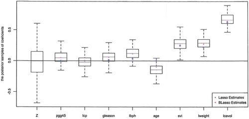
Figure 1 also includes lasso and Bayesian lasso estimates of each coefficients, marked as circles and squares in the figure. The lasso estimates are zero for pgg45, lcp, and age, nonzero for the other five covariates. Thus, the lasso approach agrees with our approach for covariates pgg45, lcp, age, svi, lweight, and lcavol, but does not agree on gleason and lbph. Since the magnitudes of lasso estimates for gleason and lbph are small, another thresholding added to lasso will result in the same conclusion with ours. Meanwhile, the Bayesian lasso evaluates all the coefficients to be nonzero as it does not select variables to promote model sparsity.

2.3. Variable selection

The benchmark serves as a measure to assess the importance of each covariate. To compare the effect of each ${\mathit{x}}_i$ with that of the benchmark $\mathit{z}$, we define the importance score $d_i$ for each ${\mathit{x}}_i$ based on the following conditional posterior probability:

(4) $d_i=P\left(\frac{|{\text{β}}_i|}{\sqrt{V\left({\text{β}}_i|\mathit{y},\mathit{X},{\sigma }^2\right)}}>\frac{|{\text{β}}_z|}{\sqrt{V\left({\text{β}}_z|\mathit{y},\mathit{X},{\sigma }^2\right)}}|\mathit{y},\mathit{X},{\sigma }^2\right)$(4) where $V\left(\xi |\mathbf{\text{A}}\right)$ denotes the posterior variance of ξ given $\mathbf{A}$. This probability could be evaluated either numerically or theoretically, depending on which prior is put on $\text{β}$. The standardisation over the variances is necessary for the purpose of fair comparison. Intuitively, a $d_i$ close to 0.5 indicates the effect of ${\mathit{x}}_i$ is not much different from the effect of the benchmark and therefore ${\mathit{x}}_i$ could be treated as an unimportant variable. With the availability of the estimated importance scores, the covariates $({\mathit{x}}_1,\dots ,{\mathit{x}}_p)$ could be ranked from the most important to the least important as $({\mathit{x}}_{\left(1\right)},\dots ,{\mathit{x}}_{\left(p\right)})$, where ${\mathit{x}}_{\left(1\right)}$ associates with the greatest estimated importance score, ${\mathit{x}}_{\left(2\right)}$ associates with the second largest importance score and etc. It is desired to select covariates that are assessed to be the most important.

Naturally, the next question to be addressed is how to determine the cutoff point $m^{\ast }$ such that only the top $m^{\ast }$ variables $({\mathit{x}}_{\left(1\right)},\dots ,{\mathit{x}}_{\left(m^{\ast }\right)})$ are selected. To avoid arbitrary thresholding on the estimated importance scores, we adopt a slighted modified BIC criterion (Chen & Chen, 2008). For each integer $m=1,\dots ,p$, the m most important covariates ${\mathit{x}}_{\left(1\right)},\dots ,{\mathit{x}}_{\left(m\right)}$ are considered in a candidate model with ${\mathit{X}}_m=({\mathit{x}}_{\left(1\right)},\dots ,{\mathit{x}}_{\left(m\right)})$. The desired cutoff point $m^{\ast }$ is the one that minimises (5) $\begin{array}{rl}\mathrm{B}\mathrm{I}\mathrm{C}\left(m\right)& =\log (\parallel \tilde{\mathit{y}}-{\mathit{X}}_m{\stackrel{\mathbf{ˆ}}{\text{β}}}_m{\parallel }^2/n)+\frac{m}{n}\left(\log n+\log p\right)\end{array}$(5) over m, where ${\stackrel{\mathbf{ˆ}}{\text{β}}}_m$ is the posterior mean of the regression parameter under model m. The original BIC in Chen and Chen (2008) uses $2\log p$ instead of $\log p$ in (5(5) $\begin{array}{rl}\mathrm{B}\mathrm{I}\mathrm{C}\left(m\right)& =\log (\parallel \tilde{\mathit{y}}-{\mathit{X}}_m{\stackrel{\mathbf{ˆ}}{\text{β}}}_m{\parallel }^2/n)+\frac{m}{n}\left(\log n+\log p\right)\end{array}$(5) ). This slight modification does not alter the asymptotic properties established in Chen and Chen (2008) but has better simulation performance in our study.

For the prostate cancer example in Section 2.2, we compute $d_i$'s and BIC$\left(m\right)$ and show them in Table 1. It can be seen that BIC$\left(m\right)$ reaches its minimum value $-0.54$ when $m^{\ast }=3$, i.e., lcavol, lweight, and svi are selected as important covariates, or equivalently, we select covariates whose $d_i$ values are over 0.9 in this example.

Table 1. Values of $d_i$ and BIC$\left(m\right)$ in prostate cancer example.

	lcavol	lweight	svi	age	lbph	gleason	lcp	pgg45
$d_i$	1.00	0.98	0.93	0.80	0.71	0.61	0.56	0.54
BIC$\left(m\right)$	−0.38	−0.47	−0.54	−0.49	−0.46	−0.41	−0.33	−0.26

2.4. Computation

The Laplace prior in (1(1) $p\left(\text{β}|{\sigma }^2\right)=\prod _{i=1}^p\frac{\lambda }{2\sigma }\exp (-\frac{\lambda |{\text{β}}_i|}{\sigma })$(1) ) is a shrinkage prior, but it is not conjugate and, hence, Bayesian computation is complicated. Fortunately, we can follow the approach in Park and Casella (2008) to carry out Bayesian computation using Gibbs sampler and to estimate λ using marginal likelihood. This is based on the fact that the Laplace distribution is a scale mixture of normal distributions where the mixing is through an exponential distribution as follows (Andrews & Mallows, 1974), (6) $\begin{array}{rl}\frac{a}{2}\exp (-a|z|)& ={\int }_0^{\mathrm{\infty }}\frac{1}{\sqrt{2\pi s}}\exp (-\frac{z^2}{2s})\frac{a^2}{2}\\ & \times \exp (-\frac{a^2}{2}s)\mathrm{d}s\end{array}$(6) Using $\mathbf{1}$ as benchmark and applying (6(6) $\begin{array}{rl}\frac{a}{2}\exp (-a|z|)& ={\int }_0^{\mathrm{\infty }}\frac{1}{\sqrt{2\pi s}}\exp (-\frac{z^2}{2s})\frac{a^2}{2}\\ & \times \exp (-\frac{a^2}{2}s)\mathrm{d}s\end{array}$(6) ), we obtain that the posterior density in (3(3) $\begin{array}{rl}& p\left(\text{β},{\text{β}}_z,{\sigma }^2|\mathit{X},\mathit{y}\right)\propto \frac{1}{{\sigma }^{n+p+3}}\\ & \times \exp \left(-\frac{{∥\tilde{\mathit{y}}-\mathit{X}\text{β}∥}^2}{2{\sigma }^2}-\frac{\lambda }{\sigma }\sum _{j=1}^p|{\text{β}}_j|-\frac{\lambda }{\sigma }|{\text{β}}_z|\right)\end{array}$(3) ) is proportional to $\begin{array}{rl}& \frac{1}{{\sigma }^{n+p+3}}\exp \left(-\frac{{∥\tilde{\mathit{y}}-\mathit{X}\text{β}∥}^2}{2{\sigma }^2}\right)\prod _{i=z,1,\dots ,p}{\int }_0^{\mathrm{\infty }}\frac{1}{{\tau }_i}\\ & \times \exp \left(-\frac{{\text{β}}_i^2}{2{\sigma }^2{\tau }_i^2}-\frac{{\lambda }^2{\tau }_i^2}{2}\right)\mathrm{d}{\tau }_i^2\end{array}$ which gives the following conditional distributions for Gibbs sampler: $\begin{array}{rl}{\text{β}}_z|\mathrm{a}\mathrm{l}\mathrm{l}\mathrm{o}\mathrm{t}\mathrm{h}\mathrm{e}\mathrm{r}\mathrm{s}& \sim N\left(0,{\tau }_z^2{\sigma }^2\right)\\ \text{β}|\mathrm{a}\mathrm{l}\mathrm{l}\mathrm{o}\mathrm{t}\mathrm{h}\mathrm{e}\mathrm{r}\mathrm{s}& \sim N\left({\mathit{A}}^{-1}{\mathit{X}}^{\prime }\tilde{\mathit{y}},{\sigma }^2{\mathit{A}}^{-1}\right)\\ {\sigma }^2|\mathrm{a}\mathrm{l}\mathrm{l}\mathrm{o}\mathrm{t}\mathrm{h}\mathrm{e}\mathrm{r}\mathrm{s}& \sim \mathrm{I}\mathrm{n}\mathrm{v}\text{-}\mathrm{G}\mathrm{a}\mathrm{m}\mathrm{m}\mathrm{a}((n+p)/2,\\ & ||\tilde{\mathit{y}}-\mathit{X}\text{β}|{|}^2/2+{\text{β}}^{\prime }{\mathit{D}}_{\tau }^{-1}\text{β}/2+{\text{β}}_z^2/2{\tau }_z^2)\\ {\tau }_i^{-2}|\mathrm{a}\mathrm{l}\mathrm{l}\mathrm{o}\mathrm{t}\mathrm{h}\mathrm{e}\mathrm{r}\mathrm{s}& \sim \mathrm{I}\mathrm{n}\mathrm{v}\text{-}\mathrm{G}\mathrm{a}\mathrm{u}\mathrm{s}\mathrm{s}\mathrm{i}\mathrm{a}\mathrm{n}\left(|\lambda \sigma /{\text{β}}_j|,{\lambda }^2\right)\\ {\tau }_z^{-2}|\mathrm{a}\mathrm{l}\mathrm{l}\mathrm{o}\mathrm{t}\mathrm{h}\mathrm{e}\mathrm{r}\mathrm{s}& \sim \mathrm{I}\mathrm{n}\mathrm{v}\text{-}\mathrm{G}\mathrm{a}\mathrm{u}\mathrm{s}\mathrm{s}\mathrm{i}\mathrm{a}\mathrm{n}\left(|\lambda \sigma /{\text{β}}_z|,{\lambda }^2\right)\end{array}$ where $\mathit{A}={\mathit{X}}^{\prime }\mathit{X}+{\mathit{D}}_{\tau }^{-1}$ and ${\mathit{D}}_{\tau }$ is a $p\times p$ diagonal matrix with ${\tau }_1^2,\dots ,{\tau }_p^2$ as diagonal components. In the kth iteration of the Gibbs sampler, the λ value estimated from the $(k-1)$th iteration is used to get the kth sample and is then updated by the kth sample as ${\hat{\lambda }}^{\left(k\right)}=\sqrt{\frac{2(p+1)}{E_{{\hat{\lambda }}^{(k-1)}}[{\tau }_z^2+\sum _{j=1}^p{\tau }_j^2|\tilde{\mathit{y}},\mathit{X}]}}$ where the conditional expectation is evaluated by the average from Gibbs samples. The derivation is omitted since it is similar to that in Park and Casella (2008).

Once the posterior samples of ${\text{β}}_z$ and $\text{β}$ are obtained, the importance score $d_i$ for each ${\mathit{x}}_i$ specified in (4(4) $d_i=P\left(\frac{|{\text{β}}_i|}{\sqrt{V\left({\text{β}}_i|\mathit{y},\mathit{X},{\sigma }^2\right)}}>\frac{|{\text{β}}_z|}{\sqrt{V\left({\text{β}}_z|\mathit{y},\mathit{X},{\sigma }^2\right)}}|\mathit{y},\mathit{X},{\sigma }^2\right)$(4) ) can be approximated by the corresponding relative frequency $\widehat{d_i}$. The ranked ${\mathit{x}}_{\left(1\right)},{\mathit{x}}_{\left(2\right)},\dots ,{\mathit{x}}_{\left(p\right)}$ can be obtained by sorting ${\hat{d}}_i$'s descendingly. Finally, we can find the cutoff point $m^{\ast }$ by minimising BIC in (5(5) $\begin{array}{rl}\mathrm{B}\mathrm{I}\mathrm{C}\left(m\right)& =\log (\parallel \tilde{\mathit{y}}-{\mathit{X}}_m{\stackrel{\mathbf{ˆ}}{\text{β}}}_m{\parallel }^2/n)+\frac{m}{n}\left(\log n+\log p\right)\end{array}$(5) ), with ${\stackrel{\mathbf{ˆ}}{\text{β}}}_m$ being the posterior mean of the regression coefficient vector when ${\mathit{X}}_m=({\mathit{x}}_{\left(1\right)},{\mathit{x}}_{\left(2\right)},\dots {\mathit{x}}_{\left(m\right)})$.

2.5. Covariates with group structures

In some studies, the covariates exhibit certain group structure. It is then desired to capture the intrinsic relation among variables within a group. In this section, we extend the idea of using a benchmark for variable selection under the Bayesian framework to accommodate the group structures. We perform variable selection in both group and individual variable levels.

Suppose that p covariates can be partitioned into G groups with sizes $p_1,\dots ,p_G$, respectively, where $\sum _{g=1}^G{p}_g=p$. The matrix $\mathit{X}$ could be written as $\mathit{X}=({\mathit{X}}_1,\dots ,{\mathit{X}}_G)$, where ${\mathit{X}}_g=({\mathit{x}}_{g1},\dots ,{\mathit{x}}_{g{p}_g})$ is a $n\times p_g$ matrix for the gth group, $g=1,\dots ,G$. The vector of associated regression coefficients can be written as ${\text{β}}^{\prime }=({\text{β}}_1^{\prime },\dots ,{\text{β}}_G^{\prime })$, where each ${\text{β}}_g^{\prime }=({\text{β}}_{g1},\dots ,{\text{β}}_{g{p}_g})$ is a vector of length $p_g$, $g=1,\dots ,G$.

The prior in (1(1) $p\left(\text{β}|{\sigma }^2\right)=\prod _{i=1}^p\frac{\lambda }{2\sigma }\exp (-\frac{\lambda |{\text{β}}_i|}{\sigma })$(1) ) does not take the group structure into consideration. Instead, as inspired by the penalty term of group lasso (Yuan & Lin, 2005), we consider the following prior density which encourages shrinkage on group level: (7) $p\left(\text{β}|{\sigma }^2\right)=\prod _{g=1}^G\frac{\lambda }{2\sigma }\exp \left(-\frac{\lambda \sqrt{p_g{\text{β}}_g^{\prime }{\text{β}}_g}}{\sigma }\right)$(7) The idea of benchmark can be extended to accommodate group level variable selection. Since a benchmark could be regarded as an individual group with a single covariate, we can assign a Laplace prior to ${\text{β}}_z$ as in Section 2.1 and consider joint prior of $({\text{β}}_z,{\text{β}}_0,\text{β},{\sigma }^2)$ as $\frac{1}{{\sigma }^2}p\left(\text{β}|{\sigma }^2\right)\frac{\lambda }{2\sigma }\exp \left(-\frac{\lambda \sqrt{{\text{β}}_z^2}}{\sigma }\right)$ where the prior of ${\text{β}}_z$ matches the form of prior for ${\text{β}}_g$ in (7(7) $p\left(\text{β}|{\sigma }^2\right)=\prod _{g=1}^G\frac{\lambda }{2\sigma }\exp \left(-\frac{\lambda \sqrt{p_g{\text{β}}_g^{\prime }{\text{β}}_g}}{\sigma }\right)$(7) ), $g=1,\dots ,G$. Since the prior does not affect the fact that $\mathbf{1}$ is a benchmark as long as the prior of ${\text{β}}_z$ has mean 0, we can still use $\mathbf{1}$ as a benchmark for group variable selection. It follows from (6(6) $\begin{array}{rl}\frac{a}{2}\exp (-a|z|)& ={\int }_0^{\mathrm{\infty }}\frac{1}{\sqrt{2\pi s}}\exp (-\frac{z^2}{2s})\frac{a^2}{2}\\ & \times \exp (-\frac{a^2}{2}s)\mathrm{d}s\end{array}$(6) ) that $\begin{array}{rl}& \exp \left(-\frac{\lambda \sqrt{p_g{\text{β}}_g^{\prime }{\text{β}}_g}}{\sigma }\right)\\ & ={\int }_0^{\mathrm{\infty }}\frac{\lambda }{\sqrt{2\pi }{\tau }_g}\exp \left(-\frac{p_g{\text{β}}_g^{\prime }{\text{β}}_g}{2{\sigma }^2{\tau }_g^2}\right)\\ & \exp \left(-\frac{{\lambda }^2}{2}{\tau }_g^2\right)d{\tau }_g^2\end{array}$ Then, after integrating out ${\text{β}}_0$, we obtain that the posterior density of $(\text{β},{\text{β}}_z,{\sigma }^2$ is proportional to $\begin{array}{rl}& \frac{1}{{\sigma }^{n+G+3}}\exp \left(-\frac{{∥\tilde{\mathit{y}}-\mathit{X}\text{β}∥}^2}{2{\sigma }^2}\right)\prod _{g=z,1,\dots ,G}{\int }_0^{\mathrm{\infty }}\frac{1}{{\tau }_g}\\ & \times \exp \left(-\frac{p_g{\text{β}}_g^{\prime }{\text{β}}_g}{2{\sigma }^2{\tau }_g^2}-\frac{{\lambda }^2{\tau }_g^2}{2}\right)\mathrm{d}{\tau }_g^2\end{array}$ which gives the following full conditional distributions: $\begin{array}{rl}{\text{β}}_z|\mathrm{a}\mathrm{l}\mathrm{l}\mathrm{o}\mathrm{t}\mathrm{h}\mathrm{e}\mathrm{r}\mathrm{s}& \sim N(0,{\tau }_z^2{\sigma }^2)\\ \text{β}|\mathrm{a}\mathrm{l}\mathrm{l}\mathrm{o}\mathrm{t}\mathrm{h}\mathrm{e}\mathrm{r}\mathrm{s}& \sim N(({\mathit{X}}^{\prime }\mathit{X}+{\mathit{D}}_{p\tau }{)}^{-1}{\mathit{X}}^{\prime }\tilde{\mathit{y}},\\ & ({\mathit{X}}^{\prime }\mathit{X}+{\mathit{D}}_{p\tau }{)}^{-1}{\sigma }^2)\\ 1/{\tau }_g^2|\mathrm{a}\mathrm{l}\mathrm{l}\mathrm{o}\mathrm{t}\mathrm{h}\mathrm{e}\mathrm{r}\mathrm{s}& \sim \mathrm{I}\mathrm{n}\mathrm{v}\text{-}\mathrm{G}\mathrm{a}\mathrm{u}\mathrm{s}\mathrm{i}\mathrm{a}\mathrm{n}(\lambda \sigma (p_g{\text{β}}_g^{\prime }{\text{β}}_g{)}^{-1/2},\\ & {\lambda }^2)\\ 1/{\tau }_z^2|\mathrm{a}\mathrm{l}\mathrm{l}\mathrm{o}\mathrm{t}\mathrm{h}\mathrm{e}\mathrm{r}\mathrm{s}& \sim \mathrm{I}\mathrm{n}\mathrm{v}\text{-}\mathrm{G}\mathrm{a}\mathrm{u}\mathrm{s}\mathrm{s}\mathrm{i}\mathrm{a}\mathrm{n}(\lambda \sigma /|{\text{β}}_z|,{\lambda }^2)\\ {\sigma }^2|\mathrm{a}\mathrm{l}\mathrm{l}\mathrm{o}\mathrm{t}\mathrm{h}\mathrm{e}\mathrm{r}\mathrm{s}& \sim \mathrm{I}\mathrm{n}\mathrm{v}\text{-}\mathrm{G}\mathrm{a}\mathrm{m}\mathrm{m}\mathrm{a}(\frac{n+G}{2},\frac{||\tilde{\mathit{y}}-\mathit{X}\text{β}|{|}^2}{2}\\ & +\frac{{\text{β}}_z^2}{2{\tau }_z^2}+\sum _{g=1}^G\frac{p_g{\text{β}}_g^{\prime }{\text{β}}_g}{2{\tau }_g^2})\end{array}$ where ${\mathit{D}}_{p\tau }$ is a diagonal matrix with each $p_g/{\tau }_g^2$ repeating $p_g$ times in order as the diagonal components, $g=1,\dots ,G$. The hyperparameter λ is estimated as in Section 2.4 with p replaced by G.

Let $b_g=\sqrt{{\text{β}}_g^{\prime }{\text{β}}_g}$, which can be regarded as a measure of the effect of group g. The gth group effect is compared with the benchmark and ranked by $d_g$ defined as (4(4) $d_i=P\left(\frac{|{\text{β}}_i|}{\sqrt{V\left({\text{β}}_i|\mathit{y},\mathit{X},{\sigma }^2\right)}}>\frac{|{\text{β}}_z|}{\sqrt{V\left({\text{β}}_z|\mathit{y},\mathit{X},{\sigma }^2\right)}}|\mathit{y},\mathit{X},{\sigma }^2\right)$(4) ) with ${\text{β}}_i$ replaced by $b_g$. These posterior probabilities can be evaluated once the posterior samples for ${\text{β}}_z$ and ${\text{β}}_g$, $g=1,\dots ,G$ are generated form Gibbs sampling. Based on these, the importance order of groups can be obtained. Like before, a BIC criterion specified in Equation (5(5) $\begin{array}{rl}\mathrm{B}\mathrm{I}\mathrm{C}\left(m\right)& =\log (\parallel \tilde{\mathit{y}}-{\mathit{X}}_m{\stackrel{\mathbf{ˆ}}{\text{β}}}_m{\parallel }^2/n)+\frac{m}{n}\left(\log n+\log p\right)\end{array}$(5) ) can be applied to eliminate groups of covariates that are unimportant.

In the procedure described above, groups are selected in an all-in-all-out fashion. However, not all of the covariates have influence on $\mathit{y}$ within an selected group. Hence, it is desired to carry out variable level selection within chosen groups. Let $\mathcal{I}$ be the index set of groups selected in the group level selection and let ${\mathit{X}}_{\mathcal{I}}=({\mathit{X}}_g,g\in \mathcal{I})$. We can apply the variable selection procedure described in Section 2.3 to the covariate vector ${\mathit{X}}_{\mathcal{I}}$. Let ${\mathit{X}}_{m^{\ast }}$ be the vector of finally selected covariates. It could happen that some groups in ${\mathit{X}}_{\mathcal{I}}$ are entirely eliminated in the variable level selection, i.e., some ${\mathit{X}}_g$'s with $g\in \mathcal{I}$ are entirely not in ${\mathit{X}}_{m^{\ast }}$. These groups are then further excluded.

Even if there is no group structure in covariates, this group level selection followed by a variable level selection can be applied for variable selection when p is very large to reduce dimensionality in a fast way because group level selection may eliminate several groups of unimportant covariates simultaneously.

3. Simulation studies

Monte Carlo simulations are carried out to compare the performance of the proposed Bayesian variable selection method via a benchmark, as well as Bayesian lasso (B-lasso) by Park and Casella (2008) and frequentist lasso by Tibshirani (1996), where the penalty parameter is tuned by 10-folds cross-validation.

In the first study, there is no group structure in covariates. Three sets of n and p with increasing ratio of p/n are considered, n = 50, p = 10, n = 50, p = 100, and n = 100, p = 500. The matrix $\mathit{X}$ is generated from multivariate normal distribution $N(\mathbf{0},\mathrm{\Sigma })$, where the $(i,j)$th element of Σ is ${.5}^{|i-j|}$, $i,j=1,\dots ,p$. Given $\mathit{X}$, the response vector $\mathit{y}$ is generated from $N(\mathit{X}{\text{β}}_0,{\sigma }_0^2\mathit{I})$, where ${\text{β}}_0=(1.5,3,0,0,2,0,\dots ,0{)}^{\prime }$ is p-dimensional with only three non-zero components (the first, second, and fifth), and ${\sigma }_0$ is chosen so that $\parallel {\text{β}}_0\parallel /{\sigma }_0$, the signal-to-noise ratio, is 3, 5, 10 when n = 50 and 3, 4, 5, 6 when n = 100. Note that the intercept ${\text{β}}_0$ is set to be 0. The covariates corresponding to non-zero ${\text{β}}_0$ components are called important covariates; otherwise they are unimportant.

We consider the following performance measures of the proposed, lasso, and B-lasso methods: (8) $\begin{array}{rl}\text{model size}& =\text{number of selected covariates }\end{array}$(8) (9) $\begin{array}{rl}\text{sensitivity}& =\frac{\begin{array}{c}\text{number of of selected important}\\ \text{covariates}\end{array}}{3}\end{array}$(9) (10) $\begin{array}{rl}\mathrm{s}\mathrm{p}\mathrm{e}\mathrm{c}\mathrm{i}\mathrm{f}\mathrm{i}\mathrm{c}\mathrm{i}\mathrm{t}\mathrm{y}& =\frac{\begin{array}{c}\text{number of removed unimportant}\\ \text{covariates}\end{array}}{p-3}\end{array}$(10) (11) $\begin{array}{rl}\mathrm{P}\mathrm{M}\mathrm{S}\mathrm{E}& =\frac{\parallel {\mathit{y}}_{\mathrm{t}\mathrm{e}\mathrm{s}\mathrm{t}}-\overline{y}-\mathit{X}\stackrel{\mathbf{ˆ}}{\text{β}}{\parallel }^2}{n}\end{array}$(11) where PMSE is estimated prediction mean square error based on a test response vector on the test response vector ${\mathit{y}}_{\mathrm{t}\mathrm{e}\mathrm{s}\mathrm{t}}$ that is independent of $\mathit{y}$ generated from $N(\mathit{X}{\text{β}}_0,{\sigma }_0^2\mathit{I})$ with the same $\mathit{X}$, and $\stackrel{\mathbf{ˆ}}{\text{β}}$ is the posterior mean under the selected model.

The averages of quantities in (8(8) $\begin{array}{rl}\text{model size}& =\text{number of selected covariates }\end{array}$(8) )–(11(11) $\begin{array}{rl}\mathrm{P}\mathrm{M}\mathrm{S}\mathrm{E}& =\frac{\parallel {\mathit{y}}_{\mathrm{t}\mathrm{e}\mathrm{s}\mathrm{t}}-\overline{y}-\mathit{X}\stackrel{\mathbf{ˆ}}{\text{β}}{\parallel }^2}{n}\end{array}$(11) ) over 1000 simulations are presented in Table 2, with simulation standard deviations given in parenthesis. In addition, the rate in 1000 simulations of selecting exactly three important covariates are also included in Table 2.

Table 2. Results for simulation Study 1.

n	p	$\frac{\parallel {\text{β}}_0\parallel }{{\sigma }_0}$	Method	Model size	Sensitivity	Specificity	PMSE	Rate
50	10	3	Proposed	2.973 (0.501)	0.955 (0.117)	0.984 (0.051)	8.022 (1.831)	0.784
			Lasso	6.032 (2.114)	0.998 (0.028)	0.566 (0.301)	8.306 (1.797)	0.104
			B-lasso	10.00 (0.000)	1.000 (0.000)	0.000 (0.000)	8.303 (1.771)	0.000
		5	Proposed	3.096 (0.356)	0.995 (0.041)	0.984 (0.048)	4.665 (0.966)	0.884
			Lasso	6.015 (2.090)	1.000 (0.011)	0.569 (0.299)	4.955 (1.044)	0.102
			B-lasso	10.00 (0.000)	1.000 (0.000)	0.000 (0.000)	4.947 (1.017)	0.000
		10	Proposed	3.123 (0.366)	1.000 (0.000)	0.982 (0.052)	2.341 (0.481)	0.890
			Lasso	5.939 (2.095)	1.000 (0.000)	0.580 (0.299)	2.502 (0.531)	0.110
			B-lasso	10.00 (0.000)	1.000 (0.000)	0.000 (0.000)	2.503 (0.515)	0.000
50	100	3	Proposed	2.891 (1.072)	0.819 (0.227)	0.996 (0.007)	9.379 (2.731)	0.327
			Lasso	17.73 (10.80)	0.990 (0.058)	0.848 (0.111)	9.758 (2.405)	0.004
			B-lasso	100.0 (0.000)	1.000 (0.000)	0.000 (0.000)	15.74 (2.935)	0.000
		5	Proposed	3.272 (0.950)	0.936 (0.142)	0.995 (0.008)	5.231 (1.665)	0.538
			Lasso	17.60 (10.50)	0.999 (0.021)	0.849 (0.108)	5.771 (1.440)	0.003
			B-lasso	100.0 (0.000)	1.000 (0.000)	0.000 (0.000)	11.86 (2.083)	0.000
		10	Proposed	3.313 (0.681)	0.996 (0.038)	0.997 (0.007)	2.374 (0.542)	0.761
			Lasso	18.58 (10.66)	1.000 (0.000)	0.839 (0.110)	2.925 (0.716)	0.002
			B-lasso	100.0 (0.000)	1.000 (0.000)	0.000 (0.000)	8.850 (1.322)	0.000
100	500	3	Proposed	3.150 (0.672)	0.970 (0.096)	1.000 (0.001)	7.588 (1.171)	0.750
			Lasso	39.08 (28.90)	1.000 (0.000)	0.928 (0.058)	9.343 (2.052)	0.000
			B-lasso	500.0 (0.000)	1.000 (0.000)	0.000 (0.000)	15.93 (1.957)	0.000
		4	Proposed	3.230 (0.601)	0.997 (0.033)	1.000 (0.001)	5.535 (0.763)	0.820
			Lasso	40.73 (28.65)	1.000 (0.000)	0.924 (0.058)	7.091 (1.580)	0.000
			B-lasso	500.0 (0.000)	1.000 (0.000)	0.000 (0.000)	13.68 (1.615)	0.000
		5	Proposed	3.180 (0.500)	1.000 (0.000)	1.000 (0.001)	4.416 (0.611)	0.860
			Lasso	42.16 (28.65)	1.000 (0.000)	0.921 (0.058)	5.693 (1.261)	0.000
			B-lasso	500.0 (0.000)	1.000 (0.000)	0.000 (0.000)	12.29 (1.400)	0.000
		6	Proposed	3.150 (0.479)	1.000 (0.000)	1.000 (0.001)	3.676 (0.507)	0.890
			Lasso	41.87 (28.24)	1.000 (0.000)	0.922 (0.057)	4.737 (1.065)	0.000
			B-lasso	500.0 (0.000)	1.000 (0.000)	0.000 (0.000)	11.34 (1.257)	0.000

Notes: Numbers in parentheses are standard deviations; the true model size is 3; model size, sensitivity, specificity, and PMSE are defined in (8(8) $\begin{array}{rl}\text{model size}& =\text{number of selected covariates }\end{array}$(8) )–(11(11) $\begin{array}{rl}\mathrm{P}\mathrm{M}\mathrm{S}\mathrm{E}& =\frac{\parallel {\mathit{y}}_{\mathrm{t}\mathrm{e}\mathrm{s}\mathrm{t}}-\overline{y}-\mathit{X}\stackrel{\mathbf{ˆ}}{\text{β}}{\parallel }^2}{n}\end{array}$(11) ); rate = rate of selecting exactly three important covariates.

The results in Table 2 illustrate substantial advantages of the proposed variable selection over the other two methods, in terms of measures in (8(8) $\begin{array}{rl}\text{model size}& =\text{number of selected covariates }\end{array}$(8) )–(11(11) $\begin{array}{rl}\mathrm{P}\mathrm{M}\mathrm{S}\mathrm{E}& =\frac{\parallel {\mathit{y}}_{\mathrm{t}\mathrm{e}\mathrm{s}\mathrm{t}}-\overline{y}-\mathit{X}\stackrel{\mathbf{ˆ}}{\text{β}}{\parallel }^2}{n}\end{array}$(11) ) and the rate of selecting exactly the three important covariates. The lasso selects much more covariates than the proposed method in all cases without improving the prediction error. The B-lasso does not select covariates, has sensitivity 1 and specificity and rate 0 and does not perform well in prediction especially when p/n is large.

In the second simulation study, a group structure is added to covariates and the proposed method in Section 2.5 is considered with a group selection followed by an individual variable selection. For comparison, we include three existing methods, the group lasso (glasso) proposed by Yuan and Lin (2006), which carries out the group level selection in an ‘all-in-all-out’ fashion, the group bridge (gbridge) proposed by Huang et al. (2009) and Zhou and Zhu (2010), which selects groups as well as individual variables, and the sparse-group lasso (sglasso) proposed by Simon et al. (2012).

Similar to the first simulation study, we generate $\mathit{X}$ from $N(\mathbf{0},\mathrm{\Sigma })$ and given $\mathit{X}$, we generate $\mathit{y}$ from $N(\mathit{X}{\text{β}}_0,{\sigma }_0^2\mathit{I})$ with $\parallel {\text{β}}_0\parallel /{\sigma }_0=3$. The group structure is from the covariance matrix Σ: components of $\mathit{X}$ within the same group have pairwise correlation 0.5, while components of $\mathit{X}$ from different groups are independent. Two cases with different sample size n, dimension p, and group structures are considered.

• Case I. n = 100 and $p=90$. There are six groups with group sizes 10, 20, 10, 20, 10, and 20, respectively. Each of groups 1, 3 and 5 contains two important covariates whose regression coefficients are 1.5 and 2, and 8 unimportant covariates. Groups 2, 4 and 6 contain all unimportant covariates. Thus, there are three important groups and a total of six important covariates.

• Case II. $n=50$ and $p=100$. There are 10 groups, each with 10 covariates. Each of groups 1 and 3 has two important covariates whose regression coefficients are 1.5 and 3, and 8 unimportant covariates. All other eight groups contain unimportant covariates. Thus, there are two important groups and a total of four important covariates.

The averages of quantities in (8(8) $\begin{array}{rl}\text{model size}& =\text{number of selected covariates }\end{array}$(8) )–(11(11) $\begin{array}{rl}\mathrm{P}\mathrm{M}\mathrm{S}\mathrm{E}& =\frac{\parallel {\mathit{y}}_{\mathrm{t}\mathrm{e}\mathrm{s}\mathrm{t}}-\overline{y}-\mathit{X}\stackrel{\mathbf{ˆ}}{\text{β}}{\parallel }^2}{n}\end{array}$(11) ) over 200 simulations are presented in Table 3 for both group and individual variable levels when (8(8) $\begin{array}{rl}\text{model size}& =\text{number of selected covariates }\end{array}$(8) )–(10(10) $\begin{array}{rl}\mathrm{s}\mathrm{p}\mathrm{e}\mathrm{c}\mathrm{i}\mathrm{f}\mathrm{i}\mathrm{c}\mathrm{i}\mathrm{t}\mathrm{y}& =\frac{\begin{array}{c}\text{number of removed unimportant}\\ \text{covariates}\end{array}}{p-3}\end{array}$(10) ) are considered, with simulation standard deviations given in parenthesis. The rate in 200 simulations of selecting exactly number of important groups and number of important individual covariates are also included in Table 3.

Table 3. Results for simulation Study 2.

		Group selection				Variable selection
Case	Method	Size	Sens	Spec	Rate	Size	Sens	Spec	Rate	PMSE
I	Proposed	3.14	1.00	0.95	0.89	6.29	1.00	1.00	0.79	3.57
		(0.46)	(0.00)	(0.15)		(0.63)	(0.00)	(0.01)		(0.52)
	glasso	3.85	1.00	0.72	0.38	46.93	1.00	0.51	0.00	5.42
		(0.89)	(0.00)	(0.30)		(17.90)	(0.00)	(0.21)		(0.89)
	gbridge	3.59	1.00	0.80	0.64	22.46	1.00	0.80	0.00	4.15
		(0.94)	(0.00)	(0.31)		(21.53)	(0.00)	(0.26)		(0.91)
	sglasso	5.50	1.00	0.17	0.04	14.66	1.00	0.90	0.01	4.56
		(0.78)	(0.00)	(0.26)		(4.97)	(0.01)	(0.06)		(0.76)
II	Proposed	1.96	0.96	1.00	0.89	3.06	0.70	1.00	0.24	13.95
		(0.32)	(0.14)	(0.03)		(1.10)	(0.24)	(0.01)		(4.49)
	glasso	3.39	1.00	0.83	0.04	33.9	1.00	0.69	0.00	17.15
		(0.64)	(0.00)	(0.08)		(6.39)	(0.00)	(0.07)		(3.84)
	gbridge	4.80	1.00	0.65	0.12	26.1	0.98	0.77	0.00	16.25
		(1.47)	(0.00)	(0.18)		(8.57)	(0.07)	(0.09)		(3.66)
	sglasso	3.89	1.00	0.76	0.35	8.14	0.90	0.95	0.05	14.13
		(2.18)	(0.00)	(0.27)		(4.77)	(0.15)	(0.05)		(3.16)

Notes: Numbers in parentheses are standard deviations; under variable selection, size = model size, sen = sensitivity, spec = specificity, defined in (8(8) $\begin{array}{rl}\text{model size}& =\text{number of selected covariates }\end{array}$(8) )–(10(10) $\begin{array}{rl}\mathrm{s}\mathrm{p}\mathrm{e}\mathrm{c}\mathrm{i}\mathrm{f}\mathrm{i}\mathrm{c}\mathrm{i}\mathrm{t}\mathrm{y}& =\frac{\begin{array}{c}\text{number of removed unimportant}\\ \text{covariates}\end{array}}{p-3}\end{array}$(10) ); under group selection, size, sen, spec are defined by (8(8) $\begin{array}{rl}\text{model size}& =\text{number of selected covariates }\end{array}$(8) )–(10(10) $\begin{array}{rl}\mathrm{s}\mathrm{p}\mathrm{e}\mathrm{c}\mathrm{i}\mathrm{f}\mathrm{i}\mathrm{c}\mathrm{i}\mathrm{t}\mathrm{y}& =\frac{\begin{array}{c}\text{number of removed unimportant}\\ \text{covariates}\end{array}}{p-3}\end{array}$(10) ) with covariates replaced by groups; PMSE is defined by (11(11) $\begin{array}{rl}\mathrm{P}\mathrm{M}\mathrm{S}\mathrm{E}& =\frac{\parallel {\mathit{y}}_{\mathrm{t}\mathrm{e}\mathrm{s}\mathrm{t}}-\overline{y}-\mathit{X}\stackrel{\mathbf{ˆ}}{\text{β}}{\parallel }^2}{n}\end{array}$(11) ); rate = rate of selecting exactly the true numbers of important groups and covariates.

The results in Table 3 demonstrate the advantage of our method in both prediction and variable selection, compared to other three methods.

4. Real data examples

For illustration, in this section, we apply the proposed method to three real datasets and compare it with other methods.

4.1. Prostate cancer

This example is introduced in Section 2.2, with variable selection illustrated in Section 2.3. To check the performance of proposed variable selection and make comparisons, we randomly split the dataset with 97 patients into 2 subsets of sizes 78 and 19, use the subset of size 78 as the training set to carry out variable selection and build regression model, and use the subset of size 19 as the test set to validate the prediction performance in terms of PMSE defined by (11(11) $\begin{array}{rl}\mathrm{P}\mathrm{M}\mathrm{S}\mathrm{E}& =\frac{\parallel {\mathit{y}}_{\mathrm{t}\mathrm{e}\mathrm{s}\mathrm{t}}-\overline{y}-\mathit{X}\stackrel{\mathbf{ˆ}}{\text{β}}{\parallel }^2}{n}\end{array}$(11) ). We independently repeat random splitting 100 times and obtain the empirical results of 100 replications in Table 4.

Table 4. Results based on 100 random splits for the prostate cancer example.

	Selection rate for each covariate
Method	lcavol	lweight	svi	age	lbph	gleason	lcp	pgg45
Proposed	1.00	0.87	0.91	0.00	0.08	0.00	0.00	0.00
Lasso	1.00	0.99	1.00	0.51	0.88	0.46	0.23	0.75
B-lasso	1.00	1.00	1.00	1.00	1.00	1.00	1.00	1.00
		Average model size				PMSE
Proposed		2.860 (0.377)				0.594 (0.189)
Lasso		5.820 (1.553)				0.600 (0.216)
B-lasso		8.000 (0.000)				0.580 (0.188)

Note: Numbers in parentheses are standard deviations.

The results in Table 4 elucidates that the proposed method outperforms lasso and B-lasso. First, the proposed selection method highly concentrates on selecting three important covariates as indicated in Figure 1 and Table 1. The average model size is 2.86. Although lasso agrees with the proposed method in selecting the three most important variables, it tends to select some redundant variables without improving PMSE, the prediction accuracy. Although Bayes lasso has a small PMSE, it does not perform variable selection.

4.2. CCT8 in a genome-wide association study

Research on linking genetic variations and phenotypic variations such as susceptibility to certain disorders is important in genomics as it helps to accelerate the understanding of genetic basis and may shed light on new medical treatments. We consider a high-dimensional dataset with p>n from a genome-wide association study, the expression quantitative trait locus (eQTL) mapping. The performance of high-resolution eQTL mapping on nucleotide level is based on the measurements of genome-wide single nucleotide polymorphism (SNP). Here we consider the eQTL mapping for the gene CCT8 measured by microarray as the response from 90 individuals, 45 Han Chinese from Beijing, China, and 45 Japanese from Tokyo, Japan. The analysis is to detect which SNPs are associated with the CCT8 expression level, from a total of 200 SNPs after an initial screening of many SNPs.

Results based on 100 random splits of the dataset similar to those in the previous example (Table 4) are given in Table 5, with 80 people in the training set and 10 in the test set. In terms of the average model size and PMSE, the results in Table 5 exhibit quite similar yet more dramatic pattern compared with the results in Table 4 for the prostate cancer data. Our variable selection method significantly promotes model sparsity by selecting only around 3.4 variables on average, whereas the lasso method selects nearly 59 variables on the average. The PMSE under our approach is not jeopardised by the simplicity of model, as it is nearly the same as the PMSE for lasso. The Bayesian lasso results in the greatest PMSE, indicating that including all 200 predictors (compared with only 8 variables in the prostate cancer example) without variable selection leads to serious prediction errors when the number of unimportant variables is overwhelming in the model.

Table 5. Results based on 100 random splits for the CCT8 example.

	Selection rate for five SNPs with the highest rates
Method	rs965951	rs2245431	rs2832321	rs16983706	rs468619
Proposed	0.73	0.48	0.44	0.28	0.34
Lasso	0.97	0.94	0.82	0.75	0.84
B-lasso	1.00	1.00	1.00	1.00	1.00
	average model size			PMSE
Proposed	3.394 (2.571)			0.035 (0.021)
Lasso	58.98 (22.93)			0.034 (0.016)
B-lasso	200.0 (0.000)			0.064 (0.037)

Note: Numbers in parentheses are standard deviations.

Over 100 random data splits, the top five most frequently selected SNPs by our approach are shown in Table 5. The highest selection frequency of SNP rs965951 suggests its relevance with the response CCT8, which is in accord with the results from some previous studies (Bradic et al., 2009; Deutsch et al., 2005; Fan et al., 2012). The second most frequently selected SNP rs2245431 was also selected by Bradic et al. (2009). All findings obtained by statistical methodologies are yet to be further validated by relevant genomical analysis.

4.3. ACS breast cancer patient OWB data

Breast cancer is a worldwide common cancer and remains the leading cause of mortality for women. With the continuously improved survival rate and prolonged life expectancy granted by advanced modern therapies, increasing efforts have been devoted to investigating the quality of life for breast cancer patients, as the quality of life plays an important role throughout the treatment and survivorship and, hence, the relevant studies may shed light on innovative intervention designs for disease control and quality of life improvement.

We consider a dataset from a large-scale breast cancer study conducted by American Cancer Society (ACS) at the School of Nursing in Indiana University. We focus on a subset of this study with 623 seniors who were 55–70 years old at diagnosis and were surveyed 3–8 years after completion of chemotherapy and surgery, with or without radiation therapy. The response of interest is overall well being (OWB), a measure captured by Campbell's index of quality of life, which is based on seven questionnaire items (Campbell et al., 2008). The objective of this study is to identify the psychological, social, and behaviour factors having important impacts on the well being of the survivors, and to establish the association between these factors and OWB.

The total 57 covariates under consideration include 3 demographic variables and 54 social or behaviour scores quantified by questionnaires which are well studied in literature (Frank-Stromborg & Olsen, 2003). The 54 social or behaviour variables are divided to 8 non-overlapping groups, which are personality, physical health, psychological health, spiritual health, active coping, passive coping, social support, and self efficacy. Each contains 4 to 12 individual covariates describing the same aspect of the social or behaviour status from different perspectives. The three demographic variables are treated as three individual groups, which are age at diagnosis, years of education, and number of months the patients were in their initial breast cancer treatment.

As in the first two examples, we randomly split the data set to a training set of size 499 and a test set of size 124, and then show the average or frequency based on 100 splits in Table 6. Similar to the second simulation study, we compare our proposed method to the glasso, gbridge, and sglasso designed for group variable selection.

Table 6. Results based on 100 random splits for the OWB example.

Method	Individual demographic variable selection
	Age	Treatment Months	Years of edu
Proposed	0.00	0.02	0.00
glasso	0.00	0.79	0.01
gbridge	0.00	0.04	0.00
sglasso	0.00	0.15	0.00
	group selection
	Personality	Physical health	Psych health	Spiritual health
	size=5	size=4	size=6	size=12
Proposed	0.00	0.00	1.00	0.21
glasso	0.01	0.90	1.00	0.20
gbridge	0.00	0.00	1.00	0.92
sglasso	0.03	0.46	1.00	0.69
	Active coping	Passive coping	Social support	Self-efficacy
	size=7	size=5	size=4	size=11
Proposed	0.04	0.05	1.00	0.05
glasso	0.33	0.02	1.00	0.43
gbridge	0.02	0.06	0.81	0.26
sglasso	0.60	0.13	1.00	0.68
	Selection within psychological health group
	ttraiAnx	tstatAnx	tbodimg	tcesd	tthinkbc
Proposed	1.00	0.98	0.79	0.64	0.70
glasso	1.00	1.00	1.00	1.00	1.00
gbridge	1.00	1.00	1.00	1.00	1.00
sglasso	1.00	1.00	0.99	1.00	0.32
	Selection within social support	Selection within spiritual health
	tcommnow	sprview6
Proposed	1.00	0.20
glasso	1.00	0.20
gbridge	0.81	0.91
sglasso	1.00	0.68
	Average of	Average of selected
	selected groups	individual variables	PMSE
Proposed	2.370 (0.646)	5.500 (1.439)	2.789 (0.448)
glasso	4.690 (0.837)	23.99 (6.889)	2.787 (0.425)
gbridge	3.110 (0.601)	10.48 (2.172)	2.713 (0.452)
sglasso	24.740 (2.008)	10.70 (4.150)	2.837 (0.424)

The first part of Table 6 shows the rate (over 100 random splits) of selecting groups, where the three individual demographic variables are treated as three groups with size 1. The psychological health group is always selected by every method, which strongly suggests its association with the response OWB. It makes intuitive sense as a diagnosis of breast cancer is the most devastating thing a woman can hear, and it is often accompanied with fear of death, loss of control, isolation, and depression (Knobf, 2007; Yoo et al., 2010), all of which make considerably negative impacts on OWB. The other group that is always selected by our method, glasso and sglasso is social support, which is characterised as combination of emotional, tangible, and informational support (Cohen et al., 2000), from any formal, informal, social, professional, structured or unstructured resources (House & Khan, 1985). Reviews on the relevant literature reveal that it has been long recognised that social support may affect the OWB of patients in chronic and life-threatening health conditions like breast cancer (Cohen & Syme, 1985). Besides the above two groups, our method also selects the spiritual health group at a relatively low frequency, while barely including any other remaining groups. Purnell and Andersen (2009) pointed out that spiritual well-being was significantly associated with quality of life and traumatic stress after controlling for disease and demographic variables. Furthermore, spirituality is regarded as a resource regularly used by patients with cancer coping with diagnosis and treatment Gall et al. (2005).

Our proposed method selects variables within each selected groups. Over 100 random data splits, the middle part of Table 6 shows the rates of top seven most frequently selected variables within the three selected groups. The selected psychological health group contains six variables, five of which are selected with high rates. In Table 6, tstatAnx and ttraiAnx are short for S-anxiety and T-anxiety scales, respectively, which are used to capture the anxiety level of patients based on 20 questions like ‘I feel nervous and restless’; tbodimg stands for body image total score and is summarised from eight questions such as ‘I am satisfied with the appearance of my body’ and ‘others find me attractive’; tcesd represents the total score for situations during the past week, and the questions associated with this construct are something like ‘I was bothered by things that usually don't bother me’ or ‘my appetite was poor’. In the social support group, only one variable is selected with high frequency, tcommnow, which quantifies the communication quality between the patients and physicians, based on questions like ‘I have a health care provider I trust’ and ‘I have a health care provider who knows me personally’. The high selection frequency of this variable is in accord with the existing research results, which suggests that although the older women obtain information regarding breast cancer from a variety of sources, they often reply heavily on their primary care physicians for support and information (Silliman et al., 1998).

While the previous analysis focuses on group and individual variable selection, the last part of Table 6 shows the advantage of our proposed method in terms of the averages of selected groups and variables, and the PMSE over 100 random splits. On the average, our method promotes model sparsity by picking only around 2.4 groups and further reduces model complexity by including less than six variables in selected groups. In contrary, both glasso and sglasso select nearly twice many groups while produce comparable PMSE. The gbridge also chooses significantly more groups than our method, while leads to a slight smaller.

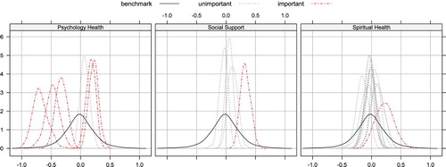
Finally, as we discussed in Section 2.2, our proposed benchmark approach can also be applied by visualising the posteriors. Figure 2 illustrates how to visualise the importance of variables within each three groups, based on the whole data set with 623 patients.

Figure 2. The posteriors of regression coefficients in three groups.

Acknowledgements

Our research was supported by the National Natural Science Foundation of China (11831008) and the U.S. National Science Foundation (DMS-1612873 and DMS-1914411). We would like to thank a referee for a careful review.

Disclosure statement

No potential conflict of interest was reported by the author(s).

Additional information

Funding

Our research was supported by the National Natural Science Foundation of China [grant number 11831008] and the U.S. National Science Foundation [grant numbers DMS-1612873 and DMS-1914411].

Notes on contributors

Jun Shao

Dr. Jun Shao holds a PhD in statistics from the University of Wisconsin-Madison. He is a Professor of Statistics at the University of Wisconsin-Madison. His research interests include variable selection and inference with high dimensional data, sample surveys, and missing data problems.

Kam-Wah Tsui

Dr. Kam-Wah Tsui is an Emeritus Professor of Statistics at the University of Wisconsin–Madison. His research interests include Bayesian analysis, sample surveys, and general statistical methodology.

Sheng Zhang

Dr. Sheng Zhang holds a Ph.D. in statistics from University of Wisconsin-Madison. She is now a data scientist at Google, Mountain View, California.

References

- Andrews, D. F., & Mallows, C. L. (1974). Scale mixtures of normal distributions. Journal of the Royal Statistical Society, Series B, 36, 99–102.
- Bayarri, M. J., Berger, J. O., Jang, W., Ray, S., Pericchi, L. R., & Visser, L. (2019). Prior-based Bayesian information criterion (PBIC). Statistical Theory and Related Fields, 3(1), 2–13. https://doi.org/10.1080/24754269.2019.1582126
- Bradic, J., Fan, J., & Wang, W. (2009). Penalized composite quasi-Likelihood for ultrahigh-Dimensional variable selection. Journal of the Royal Statistical Society, Series B, 73(3), 325–349. https://doi.org/10.1111/rssb.2011.73.issue-3
- Brown, P. J., Vannucci, M., & Fearn, T. (1998). Multivariate Bayesian variable selection and prediction. Journal of the Royal Statistical Society, Series B, 60(3), 627–641. https://doi.org/10.1111/rssb.1998.60.issue-3
- Campbell, A., Converse, P., & Rodgers, W. (2008). The quality of American life: Perceptions, evaluations, and satisfactions. Russell Sage Foundation.
- Chen, J., & Chen, Z. (2008). Extended Bayesian information criterion for model selection with large model spaces. Biometrika, 95, 759–771. https://doi.org/10.1093/biomet/asn034
- Cohen, S., Gottlieb, B., & Underwood, L. (2000). Social relationships and health. In S. Cohen, L. Underwood, & B. Gottlieb (Eds.), Social support measurement and intervention. Oxford University Press.
- Cohen, S., & Syme, L. (1985). Social support and health (Tech. Rep.). Academic.
- Dellaportas, P., Forster, J. J., & Ntzoufras, I. (1997). On Bayesian model and variable selection using MCMC (Tech. Rep.). Department of Statistics, Athens University of Economics and Business.
- Deutsch, S., Lyle, R., Dermitzakis, E., Attar, H., Subrahmanyan, L., Gehri, C., Parand, L., Gagnebin, M., Rougemont, J., Jongeneel, C., & Antonarakis, S. (2005). Gene expression variation and expression quantitative trait mapping of human chromosome 21 genes. Human Molecular Genetics, 14(23), 3741–3749. https://doi.org/10.1093/hmg/ddi404
- Dicker, L., Huang, B., & Lin, X. (2011). Variable selection and estimation with the seamless-l0 penalty. Statistica Sinica,
- Fan, J., Han, X., & Gu, W. (2012). Estimating false discovery proportion under arbitrary covariance dependence. Journal of the American Statistical Association, 107(499), 1019–1035. https://doi.org/10.1080/01621459.2012.720478
- Fan, J., & Li, R. (2001). Variable selection via nonconcave penalized likelihood and its oracle properties. Journal of the American Statistical Association, 96(456), 1348–1360. https://doi.org/10.1198/016214501753382273
- Frank-Stromborg, M., & Olsen, S. (2003). Instruments For Clinical Health-Care Research (Jones and Bartlett Series in Oncology, 3rd edition) (Tech. Rep.). Jones & Bartlett Learning.
- Gall, T., Charbonneau, C., Clarke, N., Grant, K., Joseph, A., & Shouldice, L. (2005). Understanding the nature and role of spirituality in relation to coping and health: A conceptual framework. Canadian Psychology, 46(2), 88–104. https://doi.org/10.1037/h0087008
- George, E. I., & McCulloch, R. E. (1993). Variable selection via Gibbs sampling. Journal of the American Statistical Association, 85, 398–409.
- Green, P. J. (1995). Reversible jump Markov chain Monte Carlo computation and Bayesian model determination. Biometrika, 82, 711–732. https://doi.org/10.1093/biomet/82.4.711
- Hoerl, A., & Kennard, R. (1970). Ridge regression: Biased estimation for nonorthogonal problems. Technometrics, 12(1), 55–67. https://doi.org/10.1080/00401706.1970.10488634
- Hoti, F., & Sillanpää, M. J. (2006). Bayesian mapping of genotype x expression interactions in quantitative and qualitative traits. Heredity, 97(1), 4–18. https://doi.org/10.1038/sj.hdy.6800817
- House, J., & Khan, R. (1985). Measures and concepts of social support. In S. Cohen & S. L. Syme (Eds.), Social support and health (Tech. Rep.).
- Huang, J., Ma, S., Xie, H., & Zhang, C. (2009). A group bridge approach for variable selection. Biometrika, 96, 339–355. https://doi.org/10.1093/biomet/asp020
- Knobf, M. (2007). Psychological responses in brest cancer survivors. Seminars in Oncology Nursing, 23(1), 71–83. https://doi.org/10.1016/j.soncn.2006.11.009
- Kuo, L., & Mallick, B. (1998). Variable selection for regression models. Sankhya Series B, 60, 65–81.
- Kyung, M., Gilly, J., Ghosh, M., & Casella, G. (2010). Penalized regression, standard errors, and Bayesian lassos. Bayesian Analysis, 5(2), 369–411. https://doi.org/10.1214/10-BA607
- Lin, Y., & Zhang, H. (2006). Component selection and smoothing in smoothing spline analysis of variance models. The Annals of Statistics, 34(5), 2272–2297. https://doi.org/10.1214/009053606000000722
- Lv, J., & Fan, Y. (2009). A unified approach to model selection and sparse recovery using regularized least squares. The Annals of Statistics, 37(6A), 3498–3528. https://doi.org/10.1214/09-AOS683
- O'Hara, R. B., & Sillanpää, M. J. (2009). Review of Bayesian variable selection methods: What, how and which. Bayesian Analysis, 4(1), 85–117. https://doi.org/10.1214/09-BA403
- Park, T., & Casella, G. (2008). The Bayesian Lasso. Journal of the American Statistical Association, 103(482), 681–686. https://doi.org/10.1198/016214508000000337
- Purnell, J., & Andersen, B. (2009). Religious practice and spirituality in the psychological adjustment of survivors of breast cancer. Counseling and Values, 53(3), 165–182. https://doi.org/10.1002/(ISSN)2161-007X
- Schwarz, G. (1978). Estimating the dimension of a model. The Annals of Statistics, 6(2), 461–464. https://doi.org/10.1214/aos/1176344136
- Shen, X., Pan, W., & Zhu, Y. (2011). Likelihood-based selection and sharp parameter estimation. Journal of the American Statistical Association.
- Silliman, R., Dukes, K., Sullivan, L., & Kaplan, S. (1998). Breast cancer care in older women: Sources of information, social support, and emotional health outcomes. Cancer, 83, 706–711. https://doi.org/10.1002/(ISSN)1097-0142
- Simon, N., Friedman, J., Hastie, T., & Tibshirani, R. (2012). A sparse-group lasso. Journal of Computational and Graphical Statistics.
- Stamey, T., Kabalin, J., McNeal, J., Johnstone, I., Freiha, F., Redwine, E., & Yang, N. (1989). Prostate specific antigen in the diagnosis and treatment of adenocarcinoma of the prostate.II. radical prostatectomy treated patients. Journal of Urology, 141(5), 1076–1083. https://doi.org/10.1016/S0022-5347(17)41175-X
- Tibshirani, R. (1996). Regression shrinkage and selection via the lasso. Journal of the Royal Statistical Society, Series B, 58, 267–288.
- Tibshirani, R., Saunders, M., Rosset, S., Zhu, J., & Knight, K. (2005). Sparsity and smoothness via the fused lasso. Journal of the Royal Statistical Society: Series B (Statistical Methodology), 67(1), 91–108. https://doi.org/10.1111/rssb.2005.67.issue-1
- Tipping, M. (2001). Sparse Bayesian learning and the relevance vector machine. Journal OfMachine Learning, 1, 211–244.
- Yoo, G., Levine, E., Aviv, C., Ewing, C., & Au, A. (2010). Older women, breast cancer, and social support. Supportive Care in Cancer, 18, 121521–1530. https://doi.org/10.1007/s00520-009-0774-4
- Yuan, M., & Lin, Y. (2005). Efficient empirical bayes variable selection and esimation in linear models. Journal of the American Statistical Association, 100(472), 1215–1225. https://doi.org/10.1198/016214505000000367
- Yuan, M., & Lin, Y. (2006). Model selection and estimation in regression with grouped variables. Journal of the Royal Statistical Society: Series B (Statistical Methodology), 68(1), 49–67. https://doi.org/10.1111/rssb.2006.68.issue-1
- Zhang, C. (2010). Nearly unbiased variable selection under minimax concave penalty. The Annals of Statistics, 38(2), 894–942. https://doi.org/10.1214/09-AOS729
- Zhou, N., & Zhu, J. (2010). Group variable selection via a hierarchical lasso and its oracle property. Statistics and Its Inference, 3, 557–574.
- Zou, H. (2006). The adaptive lasso and its oracle properties. Journal of the American Statistical Association, 101(476), 1418–1429. https://doi.org/10.1198/016214506000000735
- Zou, H., & Hastie, T. (2005). Regularization and variable selection via the elastic net. Journal of the Royal Statistical Society, Series B, 67(2), 301–320. https://doi.org/10.1111/rssb.2005.67.issue-2