Personalized treatment selection via the covariate-specific treatment effect curve for longitudinal data

Abstract

Treatment selection based on patient characteristics has been widely recognised in modern medicine. In this paper, we propose a generalised partially linear single-index mixed-effects modelling strategy for treatment selection and heterogeneous treatment effect estimation in longitudinal clinical and observational studies. We model the treatment effect as an unknown functional curve of a weighted linear combination of time-dependent covariates. This method enables us to investigate covariate-specific treatment effects and make personalised treatment selection in a flexible fashion. We develop a method that combines local linear regression and penalised quasi-likelihood to estimate the weight for each covariate, the unknown treatment effect curve and the parameters for mixed-effects. Based on pointwise confidence intervals for the treatment effect curve, we can make individualised treatment decisions from the information of patient characteristics. A simulation study is conducted to evaluate finite sample performance of the proposed method. We also illustrate the method via analysis of a real data example.

Keywords:

• personalized medicine
• treatment selection
• semiparametric model
• longitudinal data

1. Introduction

Personalized or precision medicine, which aims to provide treatment strategies according to the characteristics of individuals or subgroups of the population, has gained much attention from biomedical researchers. The main goal of personalised medicine is to investigate covariate-specific (heterogeneous) effects of treatment, based on which individualised clinical decision can be better made to patients. In recent years, there has been an increasing amount of literature on heterogeneous treatment effect (HTE) estimation. A typical way of exploring heterogeneous treatment effects is to examine patient outcomes in mutually exclusive subgroups defined by observable patient characteristics, see Berger et al. (2014), Ciampi et al. (1995), Negassa et al. (2005), Foster et al. (2011), Su et al. (2008) and Wang et al. (2007). Bonetti and Gelber (2004) introduced a subpopulation treatment effect pattern plot (STEPP), which characterises treatment effects across potentially overlapping intervals of a continuous covariate. Bonetti et al. (2009) indicated that this method is effective only for large sample sizes, and proposed a permutation-based method for inference and achieved better performance for smaller sample sizes. The major limitation of such subgroup approach is that dichotomisation of continuous covariates can be artificial, and thus it may lose important information from the data.

In the literature, some other works apply nonparametric and semiparametric modelling methods to study HTE. These methods impose no or very relaxed assumptions on the model structure, and thus can explore HTE in a flexible fashion. For continuous response, Foster et al. (2015) proposed a two-stage procedure. They obtain nonparametric estimates of treatment effects for each subject in stage 1, and these estimates are used to identify optimal subset for a treatment, thus determine a treatment regime in stage 2. However, this method only applies to situations that the optimal subset is contiguous. For time-to-event data, Ma and Zhou (2014) defined a covariate-specific treatment effect (CSTE) curve, which is used to represent clinical utility of a continuous biomarker. They derived estimate of CSTE curve, and constructed pointwise confidence interval to select the optimal treatment for individual patient, as well as simultaneous confidence band to identify subpopulation who respond well to a treatment. Han et al. (2017) extended the method of Ma and Zhou (2014) to the case of binary response. Both of them only considered a single biomarker. In order to incorporate multivariate or even high-dimensional covariates, Guo et al. (2018) proposed a sparse logistic single-index coefficient model for optimal treatment selection using the CSTE curve. This method offers a flexible way for studying the CSTE curve without a restrictive assumption on the structure of the curve while achieving great dimension reduction of the high-dimensional covariates.

All the above methods were proposed for cross-sectional data with responses measured at one time point. In practice, the patient outcomes are often collected at multiple follow-up times in order to better evaluate the effectiveness of treatments. In this paper, we extend the model considered in Guo et al. (2018) to the longitudinal clinical and observational studies, and consider a generalised partially linear single-index coefficient mixed-effects model (GPLSIMM) for our longitudinal setting. Similar as Guo et al. (2018), we treat the treatment effect as an unknown functional curve of a weighted linear combination of time-varying covariates. The weights for covariates account for their different contributions to the treatment effect, and they are estimated from the data. In longitudinal studies, the repeated measures are correlated within subjects, and thus the estimating method considered in Guo et al. (2018) is not applicable to our proposed GPLSIMM. In our model, we need to estimate the unknown functional curve, the weight of each covariate and the parameters for the mixed-effects. Estimation of generalised semiparametric mixed-effects models has been considered in some existing works. Liang (2009) proposed a local linear regression and penalised quasi-likelihood method for estimation of a generalised partially linear mixed-effects model. Pang and Xue (2012) considered a local linear regression with GEE method for a single-index mixed effects model. Xu and Zhu (2012) and Chen et al. (2014) developed a kernel and a P-spline estimation method, respectively, together with quasi-lilikelhood for longitudinal generalised single-index models.

Based on the methods considered in these works, we see that penalised quasi-likelihood is a commonly used method for estimation of generalised mixed-effects models. It circumvents the calculation of high-dimensional integral in likelihood function (Breslow & Clayton, 1993). In our proposed GPLSIMM, we approximate the unknown treatment effect curve by the local linear method and estimate the parameters for the parametric and nonparametric parts through alternatively optimising the local and global penalised quasi-likelihood functions. We then select optimal treatment for a future patient based on pointwise confidence intervals for the CSTE curve.

The rest of the paper is organised as follows. In Section 2, we introduce the proposed model, the CSTE curve and the estimation method. Section 3 gives asymptotic properties of parametric and nonparametric estimates. Section 4 provides the algorithm for model estimation. In Section 5 we evaluate the finite sample properties of the proposed method via simulation studies, while Section 6 illustrates the application of the proposed method in a real data set. All technical proofs are relegated to Appendix.

2. Model and estimation

2.1. Model

Suppose our data are obtained from n independent subjects, and observations of the ith subject is $\left\{\right(Y_{ij},X_{ij},Z_{ij},A_{ij},D_{ij}),j=1,\dots ,n_i\}$. $Y_{ij}$ is the response, $X_{ij}$, $Z_{ij}$ and $A_{ij}$ are covariates of dimension p, q and s, and $D_{ij}\in \{0,1\}$ is an indicator of exposure to treatment. We assume the relationship of response and covariates is specified by the following GPLSIMM: (1) $\begin{array}{rl}& \mathrm{E}(Y_{ij}|X_{ij},Z_{ij},A_{ij},D_{ij},{\gamma \gamma }_i)\\ & =g^{-1}\{{\alpha \alpha }^{\mathrm{T}}{X}_{ij}+f({\text{β}\text{β}}^{\mathrm{T}}{Z}_{ij})D_{ij}+A_{ij}^{\mathrm{T}}{\gamma \gamma }_i\},\\ & \mathrm{v}\mathrm{a}\mathrm{r}(Y_{ij}|X_{ij},Z_{ij},A_{ij},D_{ij},{\gamma \gamma }_i)\\ & =w_{ij}^{-1}\phi V\left({\mu }_{ij}\right),i=1,\dots ,n,j=1,\dots ,n_i,\end{array}$(1) where ${\mu }_{ij}=\mathrm{E}(Y_{ij}|X_{ij},Z_{ij},A_{ij},D_{ij},{\gamma \gamma }_i)$, $g(\cdot )$ and $V(\cdot )$ are known functions, φ is a scale parameter and $w_{ij}$ is a pre-determined weight for the jth observation of the ith subject. $f(\cdot )$ is an unknown function, and $\alpha \alpha$ and $\text{β}\text{β}$ are unknown parameter vectors. For model identifiability, we assume that $\parallel \text{β}\text{β}\parallel =1$ and ${\text{β}}_1>0$. We incorporate random effect $A_{ij}^{\mathrm{T}}{\gamma \gamma }_i$ to account for the within-subject correlation, where ${\gamma \gamma }_i,i=1,\dots ,n$ are $s$-dimensional random effect vectors. We assume that ${\gamma \gamma }_i\sim N(00,GG)$.

In this model, we characterise the treatment effect with a single-index term $f\left({\text{β}\text{β}}^{\mathrm{T}}{Z}_{ij}\right)$, and the relationship of response and covariates for control group with a generalised linear mixed effect model. When response Y is binary, we can easily see that (2) $\begin{array}{rl}f\left({\text{β}\text{β}}^{\mathrm{T}}Z\right)& =\mathrm{l}\mathrm{o}\mathrm{g}\mathrm{i}\mathrm{t}\left\{\mathrm{E}\right(Y|X,Z,A,\gamma \gamma ,D=1\left)\right\}\\ & -\mathrm{l}\mathrm{o}\mathrm{g}\mathrm{i}\mathrm{t}\left\{\mathrm{E}\right(Y|X,Z,A,\gamma \gamma ,D=0\left)\right\}.\end{array}$(2) When Y is a count variable and follows Poisson distribution, (3) $\begin{array}{rl}f\left({\text{β}\text{β}}^{\mathrm{T}}Z\right)& =\log \left\{\mathrm{E}\right(Y|X,Z,A,\gamma \gamma ,D=1\left)\right\}\\ & -\log \left\{\mathrm{E}\right(Y|X,Z,A,\gamma \gamma ,D=0\left)\right\}.\end{array}$(3) Assume that D = 0 and D = 1 represents standard care and treatment respectively, X and Z are patient characteristics, Y indicates outcome of the study, and the better outcome corresponds to larger value of Y. From (2(2) $\begin{array}{rl}f\left({\text{β}\text{β}}^{\mathrm{T}}Z\right)& =\mathrm{l}\mathrm{o}\mathrm{g}\mathrm{i}\mathrm{t}\left\{\mathrm{E}\right(Y|X,Z,A,\gamma \gamma ,D=1\left)\right\}\\ & -\mathrm{l}\mathrm{o}\mathrm{g}\mathrm{i}\mathrm{t}\left\{\mathrm{E}\right(Y|X,Z,A,\gamma \gamma ,D=0\left)\right\}.\end{array}$(2) ) and (3(3) $\begin{array}{rl}f\left({\text{β}\text{β}}^{\mathrm{T}}Z\right)& =\log \left\{\mathrm{E}\right(Y|X,Z,A,\gamma \gamma ,D=1\left)\right\}\\ & -\log \left\{\mathrm{E}\right(Y|X,Z,A,\gamma \gamma ,D=0\left)\right\}.\end{array}$(3) ), $f\left({\text{β}\text{β}}^{\mathrm{T}}Z\right)$ could be regarded as a measure of treatment effect. We define $f(\cdot )$ as covariate-specific treatment effect (CSTE) curve under this model.

Given the estimate and confidence interval of $f(\cdot )$, we could suggest the optimal treatment for a future patient based on his or her personal characteristics. Taking binary response as an example, we assume that Y = 1 represent a disease being cured, while Y = 0 indicate uncured. Let $u_0$ be the estimated value of ${\theta \theta }^{\mathrm{T}}Z$ calculated from personal characteristics of a patient. If the lower bound of confidence interval for $f\left(u_0\right)$ is greater than 0, the treatment is more effective than standard care for the patient. On the other hand, if the upper bound of confidence interval is smaller than 0, standard care is more effective. In this case, we could not recommend the treatment to the patient. If neither of the above cases happen, that is, 0 is contained in the confidence interval, we would draw the conclusion that there's no significant difference between treatment and standard care.

2.2. Estimation

Denote $\mathrm{\Gamma }\mathrm{\Gamma }=({\gamma }_1^{\mathrm{T}},\dots ,{\gamma }_n^{\mathrm{T}}{)}^{\mathrm{T}}$. Let ${\text{β}\text{β}}^{\left(1\right)}=({\text{β}}_2,\dots ,{\text{β}}_q{)}^{\mathrm{T}}$ be the vector after deleting the first element from $\text{β}\text{β}$. Then $\text{β}\text{β}=(\sqrt{1-\parallel {\text{β}\text{β}}^{\left(1\right)}{\parallel }^2},{\text{β}\text{β}}^{\left(1\right)\mathrm{T}}{)}^{\mathrm{T}}$, and we define the Jacobian matrix $JJ={JJ}_{{\text{β}\text{β}}^{\left(1\right)}}=\frac{\mathrm{\partial }\text{β}\text{β}}{\mathrm{\partial }{\text{β}\text{β}}^{\left(1\right)\mathrm{T}}}=\left(\begin{array}{c}-\frac{{\text{β}\text{β}}^{\left(1\right)\mathrm{T}}}{\sqrt{1-\parallel {\text{β}\text{β}}^{\left(1\right)}{\parallel }^2}}\\ {II}_{q-1}\end{array}\right).$ Our primary interest is to estimate $f(\cdot )$, $\alpha \alpha$, $\text{β}\text{β}$ and $GG$.

Suppose that $GG$ is known. Given $\alpha \alpha$ and $\text{β}\text{β}$, we combine penalised quasi-likelihood with local linear technique to obtain estimates of $f(\cdot )$ and $f^{\mathrm{\prime }}(\cdot )$. If u is in a neighbourhood of ${\text{β}\text{β}}^{\mathrm{T}}{Z}_{ij}$, $g\left({\mu }_{ij}\right)$ can be approximated by $\begin{array}{rl}g\left({\tilde{\mu }}_{ij}\right)& ={\alpha \alpha }^{\mathrm{T}}{X}_{ij}+\left\{f\right(u)+f^{\mathrm{\prime }}(u\left)\right({\text{β}\text{β}}^{\mathrm{T}}{Z}_{ij}-u\left)\right\}{D}_{ij}\\ & +A_{ij}^{\mathrm{T}}{\gamma \gamma }_i.\end{array}$ Let $\mathrm{d}(y,\mu )=-2{\int }_y^{\mu }\left(\right(y-u\left)/V\left(u\right)\right)\mathrm{d}u$, $K_h(\cdot )=h^{-1}K(\cdot /h)$, where h is bandwidth, $K(\cdot )$ is a zero-mean symmetric density function. We maximise the following local penalised quasi-likelihood (4) $\begin{array}{rl}& -\frac{1}{2}\sum _{i=1}^n\left\{\sum _{j=1}^{n_i}{K}_h({\text{β}\text{β}}^{\mathrm{T}}{Z}_{ij}-u)w_{ij}{\phi }^{-1}\mathrm{d}(Y_{ij},g^{-1}[{\alpha \alpha }^{\mathrm{T}}{X}_{ij}\right.\\ & \left.\phantom{\sum _{j=1}^{n_i}}+\{a+b({\text{β}\text{β}}^{\mathrm{T}}{Z}_{ij}-u\left)\right\}{D}_{ij}+A_{ij}^{\mathrm{T}}{\gamma \gamma }_i])+{\gamma \gamma }_i^{\mathrm{T}}{GG}^{-1}{\gamma \gamma }_i\right\}\end{array}$(4) with respect to a, b and $\mathrm{\Gamma }\mathrm{\Gamma }$, and obtain estimates $\hat{f}\left(u\right)=\hat{a}$ and ${\hat{f}}^{\mathrm{\prime }}\left(u\right)=\hat{b}$. Taking derivative on (4(4) $\begin{array}{rl}& -\frac{1}{2}\sum _{i=1}^n\left\{\sum _{j=1}^{n_i}{K}_h({\text{β}\text{β}}^{\mathrm{T}}{Z}_{ij}-u)w_{ij}{\phi }^{-1}\mathrm{d}(Y_{ij},g^{-1}[{\alpha \alpha }^{\mathrm{T}}{X}_{ij}\right.\\ & \left.\phantom{\sum _{j=1}^{n_i}}+\{a+b({\text{β}\text{β}}^{\mathrm{T}}{Z}_{ij}-u\left)\right\}{D}_{ij}+A_{ij}^{\mathrm{T}}{\gamma \gamma }_i])+{\gamma \gamma }_i^{\mathrm{T}}{GG}^{-1}{\gamma \gamma }_i\right\}\end{array}$(4) ) with respect to $(a,b)$ and $\mathrm{\Gamma }\mathrm{\Gamma }$ yields the following estimating equations: (5) $\begin{array}{rl}& \sum _{i=1}^n\sum _{j=1}^{n_i}{K}_h({\text{β}\text{β}}^{\mathrm{T}}{Z}_{ij}-u)\left\{g^{\mathrm{\prime }}\right({\tilde{\mu }}_{ij}\left){\}}^{-1}{w}_{ij}{\phi }^{-1}{V}^{-1}\right({\tilde{\mu }}_{ij})\\ & \times \left(Y_{ij}-g^{-1}[{\alpha \alpha }^{\mathrm{T}}{X}_{ij}+\{a+b({\text{β}\text{β}}^{\mathrm{T}}{Z}_{ij}-u)\}{D}_{ij}\right.\\ & \left.+A_{ij}^{\mathrm{T}}{\gamma \gamma }_i]\right)D_{ij}\left(\begin{array}{c}1\\ {\text{β}\text{β}}^{\mathrm{T}}{Z}_{ij}-u\end{array}\right)=00,\end{array}$(5) and for each i, (6) $\begin{array}{rl}& \sum _{j=1}^{n_i}{K}_h({\text{β}\text{β}}^{\mathrm{T}}{Z}_{ij}-u)A_{ij}\left\{g^{\mathrm{\prime }}\right({\tilde{\mu }}_{ij}\left){\}}^{-1}{w}_{ij}{\phi }^{-1}{V}^{-1}\right({\tilde{\mu }}_{ij})\\ & \times \left(Y_{ij}-g^{-1}[{\alpha \alpha }^{\mathrm{T}}{X}_{ij}+\{a+b({\text{β}\text{β}}^{\mathrm{T}}{Z}_{ij}-u)\}{D}_{ij}\right.\\ & \left.+A_{ij}^{\mathrm{T}}{\gamma \gamma }_i]\right)-{GG}^{-1}{\gamma \gamma }_i=00.\end{array}$(6)

When $f(\cdot )$ is known, we obtain estimate of $\alpha \alpha$, $\text{β}\text{β}$ and $\mathrm{\Gamma }\mathrm{\Gamma }$ by maximising the global penalised quasi-likelihood (7) $\begin{array}{rl}& -\frac{1}{2}\sum _{i=1}^n\left(\sum _{j=1}^{n_i}{w}_{ij}{\phi }^{-1}d[Y_{ij},g^{-1}\{{\alpha \alpha }^{\mathrm{T}}{X}_{ij}+f({\text{β}\text{β}}^{\mathrm{T}}{Z}_{ij})D_{ij}\right.\\ & \left.\phantom{\sum _{j=1}^{n_i}}+A_{ij}^{\mathrm{T}}{\gamma \gamma }_i\}]+{\gamma \gamma }_i^{\mathrm{T}}{GG}^{-1}{\gamma \gamma }_i\right),\end{array}$(7) with respect to $\alpha \alpha$, ${\text{β}\text{β}}^{\left(1\right)}$ and $\mathrm{\Gamma }\mathrm{\Gamma }$. The corresponding estimating equations are as follows: (8) $\begin{array}{rl}& {SS}_{01}(\alpha \alpha ,{\text{β}\text{β}}^{\left(1\right)},\mathrm{\Gamma }\mathrm{\Gamma })\\ & =\sum _{i=1}^n\sum _{j=1}^{n_i}{X}_{ij}\left\{g^{\mathrm{\prime }}\right({\mu }_{ij}\left){\}}^{-1}{w}_{ij}{\phi }^{-1}{V}^{-1}\right({\mu }_{ij})\\ & \times \left[Y_{ij}-g^{-1}\{{\alpha \alpha }^{\mathrm{T}}{X}_{ij}+f({\text{β}\text{β}}^{\mathrm{T}}{Z}_{ij})D_{ij}+A_{ij}^{\mathrm{T}}{\gamma \gamma }_i\}\right]\\ & =00,\end{array}$(8) (9) $\begin{array}{rl}& {SS}_{02}(\alpha \alpha ,{\text{β}\text{β}}^{\left(1\right)},\mathrm{\Gamma }\mathrm{\Gamma })\\ & =\sum _{i=1}^n\sum _{j=1}^{n_i}{JJ}_{{\text{β}\text{β}}^{\left(1\right)}}^{\mathrm{T}}{Z}_{ij}{D}_{ij}{f}^{\mathrm{\prime }}\left({\text{β}\text{β}}^{\mathrm{T}}{Z}_{ij}\right)\left\{g^{\mathrm{\prime }}\right({\mu }_{ij}){\}}^{-1}{w}_{ij}{\phi }^{-1}\\ & +V^{-1}\left({\mu }_{ij}\right)\left[Y_{ij}-g^{-1}\left\{{\alpha \alpha }^{\mathrm{T}}{X}_{ij}f\right({\text{β}\text{β}}^{\mathrm{T}}{Z}_{ij})D_{ij}+A_{ij}^{\mathrm{T}}{\gamma \gamma }_i\}\right]\\ & =00,\end{array}$(9) and for each $i=1,\dots ,n$, (10) $\begin{array}{rl}& {SS}_i(\alpha \alpha ,{\text{β}\text{β}}^{\left(1\right)},{\gamma \gamma }_i)\\ & =\sum _{j=1}^{n_i}{A}_{ij}\left\{g^{\mathrm{\prime }}\right({\mu }_{ij}\left){\}}^{-1}{w}_{ij}{\phi }^{-1}{V}^{-1}\right({\mu }_{ij})\\ & \times \left[Y_{ij}-g^{-1}\{{\alpha \alpha }^{\mathrm{T}}{X}_{ij}+f({\text{β}\text{β}}^{\mathrm{T}}{Z}_{ij})D_{ij}+A_{ij}^{\mathrm{T}}{\gamma \gamma }_i\}\right]\\ & -{GG}^{-1}{\gamma \gamma }_i\\ & =00.\end{array}$(10)

We obtain the parametric and nonparametric estimates by iteratively maximising quasi-likelihoods (4(4) $\begin{array}{rl}& -\frac{1}{2}\sum _{i=1}^n\left\{\sum _{j=1}^{n_i}{K}_h({\text{β}\text{β}}^{\mathrm{T}}{Z}_{ij}-u)w_{ij}{\phi }^{-1}\mathrm{d}(Y_{ij},g^{-1}[{\alpha \alpha }^{\mathrm{T}}{X}_{ij}\right.\\ & \left.\phantom{\sum _{j=1}^{n_i}}+\{a+b({\text{β}\text{β}}^{\mathrm{T}}{Z}_{ij}-u\left)\right\}{D}_{ij}+A_{ij}^{\mathrm{T}}{\gamma \gamma }_i])+{\gamma \gamma }_i^{\mathrm{T}}{GG}^{-1}{\gamma \gamma }_i\right\}\end{array}$(4) ) and (7(7) $\begin{array}{rl}& -\frac{1}{2}\sum _{i=1}^n\left(\sum _{j=1}^{n_i}{w}_{ij}{\phi }^{-1}d[Y_{ij},g^{-1}\{{\alpha \alpha }^{\mathrm{T}}{X}_{ij}+f({\text{β}\text{β}}^{\mathrm{T}}{Z}_{ij})D_{ij}\right.\\ & \left.\phantom{\sum _{j=1}^{n_i}}+A_{ij}^{\mathrm{T}}{\gamma \gamma }_i\}]+{\gamma \gamma }_i^{\mathrm{T}}{GG}^{-1}{\gamma \gamma }_i\right),\end{array}$(7) ). The corresponding algorithm is summarised in Section 4 for practical implementation.

3. Asymptotic properties

Denote $q_k(t,y)=-\frac{1}{2}\left({\mathrm{\partial }}^{k}d\{y,g^{-1}(t\left)\right\}/\mathrm{\partial }{t}^k\right)$, and ${\rho }_k\left(t\right)=\left\{\mathrm{d}{g}^{-1}\left(t\right)/\mathrm{d}t{\}}^k{V}^{-1}\right\{g^{-1}\left(t\right)\}$, k = 1, 2, 3. Let ${\kappa }_j=\int u^{j}K\left(u\right)\mathrm{d}u,{\mu }_j=\int u^j{K}^2\left(u\right)\mathrm{d}u$ for j = 1, 2, $N=\sum _{i=1}^n{n}_i$ and $N_1=\sum _{i=1}^n{n}_i(n_i-1)$. We assume n tends to infinity and $n_i$'s are bounded. Denote ${\eta }_{ij}={\alpha \alpha }^{\mathrm{T}}{X}_{ij}+f\left({\text{β}\text{β}}^{\mathrm{T}}{Z}_{ij}\right)D_{ij}+A_{ij}^{\mathrm{T}}{\gamma \gamma }_i$, and $\eta ={\alpha \alpha }^{\mathrm{T}}X+f\left({\text{β}\text{β}}^{\mathrm{T}}Z\right)D+A^{\mathrm{T}}\gamma \gamma$.

In order to obtain asymptotic behaviours of the proposed parametric and nonparametric estimates, we assume the following regularity conditions:

1. The marginal density of Z is positive and uniformly continuous with a compact support $\mathcal{Z}\subseteq {\mathbb{R}}^q$. $f_{\mathcal{U}}(\cdot )$, density function of $U={\text{β}\text{β}}^{\mathrm{T}}Z$, is twice continuously differentiable for $U\in \mathcal{U}$, where $\mathcal{U}=[b_1,b_2]=\{{\text{β}\text{β}}^{\mathrm{T}}Z,Z\in \mathcal{Z}\}$ is a compact interval.

2. For all x, ${\rho }_2\left(x\right)>0$.

3. The second derivative of $g(\cdot ),V(\cdot )$ and $f(\cdot )$ are bounded and continuous.

4. The kernel $K(\cdot )$ is a bounded and symmetric probability density function with bounded support $[-c_0,c_0]$, and satisfies $\int u^{2}K\left(u\right)\mathrm{d}u\ne 0$ and $\int u^{2}K\left(u\right)\mathrm{d}u<\mathrm{\infty }$. $K(\cdot )$ satisfies the Lipschitz condition of order 1.

5. $\mathrm{E}\left\{{\rho }_2\right(\eta )D^2|{\text{β}\text{β}}^{\mathrm{T}}Z=u\},\mathrm{E}\left\{{\rho }_2\right(\eta )DX|{\text{β}\text{β}}^{\mathrm{T}}Z=u\}$ and $\mathrm{E}\left\{{\rho }_2\right(\eta )D^{2}Z|{\text{β}\text{β}}^{\mathrm{T}}Z=u\}$ are twice differentiable on u. $\mathrm{E}\left\{q_1\right({\eta }_{11},Y_{11}\left)q_1\right({\eta }_{12},Y_{12})D_{11}^2{D}_{12}^2|{\text{β}\text{β}}^{\mathrm{T}}{Z}_{11}=u_1,{\text{β}\text{β}}^{\mathrm{T}}{Z}_{12}=u_2\}$ is continuous on $u_1$ and $u_2$.

6. As $n\to \mathrm{\infty }$, h satisfies $n{h}^4\to 0$ and $n{h}^2/\log \left(1/h\right)\to \mathrm{\infty }$.

Denote $\begin{array}{rl}\tilde{X}& =X-{\left[\mathrm{E}\left\{{\rho }_2\right(\eta \left)D^2|{\text{β}\text{β}}^{\mathrm{T}}Z\right\}\right]}^{-1}\left[\mathrm{E}\left\{{\rho }_2\right(\eta \left)DX|{\text{β}\text{β}}^{\mathrm{T}}Z\right\}\right],\\ \tilde{Z}& =f^{\mathrm{\prime }}\left({\text{β}\text{β}}^{\mathrm{T}}Z\right){JJ}^{\mathrm{T}}\left(Z-{\left[\mathrm{E}\left\{{\rho }_2\right(\eta \left)D^2|{\text{β}\text{β}}^{\mathrm{T}}Z\right\}\right]}^{-1}\right.\\ & \times \left.\left[\mathrm{E}\left\{{\rho }_2\right(\eta \left)D^{2}Z|{\text{β}\text{β}}^{\mathrm{T}}Z\right\}\right]\right).\end{array}$ Let $\widehat{\alpha \alpha },\widehat{\text{β}\text{β}}$ be the final estimator of $\alpha \alpha$ and $\text{β}\text{β}$, respectively. Theorem 3.1 gives the asymptotic distributions of $\widehat{\alpha \alpha }$ and $\widehat{\text{β}\text{β}}$.

Theorem 3.1

Under conditions (C1)–(C6), (11) $\sqrt{N}\left(\begin{array}{c}\widehat{\alpha \alpha }-{\alpha \alpha }_0\\ \widehat{\text{β}\text{β}}-{\text{β}\text{β}}_0\end{array}\right)\to N(0,\mathrm{\Sigma }\mathrm{\Sigma }),$(11) where $\begin{array}{r}\mathrm{\Sigma }\mathrm{\Sigma }=\mathcal{D}\left({\mathcal{A}}^{-1}+\frac{N_1}{N}{\mathcal{A}}^{-1}\mathcal{C}{\mathcal{A}}^{-1}\right){\mathcal{D}}^{\mathrm{T}},\end{array}$ with $\begin{array}{rl}\mathcal{A}& =\mathrm{E}\left\{{\rho }_2\left(\eta \right){\left(\begin{array}{c}\tilde{X}\\ \tilde{Z}D\end{array}\right)}^{\otimes 2}\right\},\\ \mathcal{C}& =\text{cov}\left\{\left(\begin{array}{c}{\tilde{X}}_{11}\\ {\tilde{Z}}_{11}{D}_{11}\end{array}\right)q_1({\eta }_{11},Y_{11}),\right.\\ & \left.\left(\begin{array}{c}{\tilde{X}}_{12}\\ {\tilde{Z}}_{12}{D}_{12}\end{array}\right)q_1({\eta }_{12},Y_{12})\right\},\end{array}$ and $\mathcal{D}=\left(\begin{array}{cc}{II}_p& {00}_{p\times (q-1)}\\ {00}_{q\times p}& {JJ}_{{\text{β}\text{β}}_0^{\left(1\right)}}\end{array}\right).$

Theorem 3.1 indicates that in order to obtain $\sqrt{n}-$consistent estimates of $\alpha \alpha$ and $\text{β}\text{β}$, we need to undersmooth the nonparametric function $f(\cdot )$. For any $z\in \mathcal{Z}$, we let $\hat{f}({\widehat{\text{β}\text{β}}}^{\mathrm{T}}z;\widehat{\alpha \alpha },\widehat{\text{β}\text{β}})$ be the estimate of $f\left({\text{β}\text{β}}^{\mathrm{T}}z\right)$ given $\widehat{\alpha \alpha },\widehat{\text{β}\text{β}}$ and $h_1$ be the corresponding bandwidth. Theorem 3.2 presents the asymptotic distribution of $\hat{f}({\widehat{\text{β}\text{β}}}^{\mathrm{T}}z;\widehat{\alpha \alpha },\widehat{\text{β}\text{β}})$.

Theorem 3.2

Under conditions (C1)–(C5), as $n\to \mathrm{\infty },$ $h_1\to 0$ and $N{h}_1\to \mathrm{\infty }$, (12) $\begin{array}{rl}& \sqrt{Nh}\left\{\hat{f}\right({\widehat{\text{β}\text{β}}}^{\mathrm{T}}z;\widehat{\alpha \alpha },\widehat{\text{β}\text{β}})-f({\text{β}\text{β}}_0^{\mathrm{T}}z)-\frac{1}{2}{h}^2{\kappa }_2{f}^{\mathrm{\prime }\mathrm{\prime }}({\text{β}\text{β}}_0^{\mathrm{T}}z\left)\right\}\\ & \to N(0,{\sigma }_f^2),\end{array}$(12) where ${\sigma }_f^2={\mu }_0{f}_{\mathcal{U}}^{-1}\left({\text{β}\text{β}}_0^{\mathrm{T}}z\right)\left[\mathrm{E}\right\{{\rho }_2\left(\eta \right)D^2|{\text{β}\text{β}}_0^{\mathrm{T}}Z={\text{β}\text{β}}_0^{\mathrm{T}}z\}{]}^{-1}$.

4. Computation

Given $\alpha \alpha$ and $\text{β}\text{β}$, we solve estimating Equations (5(5) $\begin{array}{rl}& \sum _{i=1}^n\sum _{j=1}^{n_i}{K}_h({\text{β}\text{β}}^{\mathrm{T}}{Z}_{ij}-u)\left\{g^{\mathrm{\prime }}\right({\tilde{\mu }}_{ij}\left){\}}^{-1}{w}_{ij}{\phi }^{-1}{V}^{-1}\right({\tilde{\mu }}_{ij})\\ & \times \left(Y_{ij}-g^{-1}[{\alpha \alpha }^{\mathrm{T}}{X}_{ij}+\{a+b({\text{β}\text{β}}^{\mathrm{T}}{Z}_{ij}-u)\}{D}_{ij}\right.\\ & \left.+A_{ij}^{\mathrm{T}}{\gamma \gamma }_i]\right)D_{ij}\left(\begin{array}{c}1\\ {\text{β}\text{β}}^{\mathrm{T}}{Z}_{ij}-u\end{array}\right)=00,\end{array}$(5) ) and (6(6) $\begin{array}{rl}& \sum _{j=1}^{n_i}{K}_h({\text{β}\text{β}}^{\mathrm{T}}{Z}_{ij}-u)A_{ij}\left\{g^{\mathrm{\prime }}\right({\tilde{\mu }}_{ij}\left){\}}^{-1}{w}_{ij}{\phi }^{-1}{V}^{-1}\right({\tilde{\mu }}_{ij})\\ & \times \left(Y_{ij}-g^{-1}[{\alpha \alpha }^{\mathrm{T}}{X}_{ij}+\{a+b({\text{β}\text{β}}^{\mathrm{T}}{Z}_{ij}-u)\}{D}_{ij}\right.\\ & \left.+A_{ij}^{\mathrm{T}}{\gamma \gamma }_i]\right)-{GG}^{-1}{\gamma \gamma }_i=00.\end{array}$(6) ) by Fisher's scoring algorithm (see Wu & Zhang, 2006, Section 10.4), and obtain estimates $\hat{f}(\cdot )$ and ${\hat{f}}^{\mathrm{\prime }}(\cdot )$.

When $f(\cdot )$ is given, we obtain estimates of $\alpha \alpha$, ${\text{β}\text{β}}^{\left(1\right)}$ and $\mathrm{\Gamma }\mathrm{\Gamma }$ by solving Equations (8(8) $\begin{array}{rl}& {SS}_{01}(\alpha \alpha ,{\text{β}\text{β}}^{\left(1\right)},\mathrm{\Gamma }\mathrm{\Gamma })\\ & =\sum _{i=1}^n\sum _{j=1}^{n_i}{X}_{ij}\left\{g^{\mathrm{\prime }}\right({\mu }_{ij}\left){\}}^{-1}{w}_{ij}{\phi }^{-1}{V}^{-1}\right({\mu }_{ij})\\ & \times \left[Y_{ij}-g^{-1}\{{\alpha \alpha }^{\mathrm{T}}{X}_{ij}+f({\text{β}\text{β}}^{\mathrm{T}}{Z}_{ij})D_{ij}+A_{ij}^{\mathrm{T}}{\gamma \gamma }_i\}\right]\\ & =00,\end{array}$(8) ), (9(9) $\begin{array}{rl}& {SS}_{02}(\alpha \alpha ,{\text{β}\text{β}}^{\left(1\right)},\mathrm{\Gamma }\mathrm{\Gamma })\\ & =\sum _{i=1}^n\sum _{j=1}^{n_i}{JJ}_{{\text{β}\text{β}}^{\left(1\right)}}^{\mathrm{T}}{Z}_{ij}{D}_{ij}{f}^{\mathrm{\prime }}\left({\text{β}\text{β}}^{\mathrm{T}}{Z}_{ij}\right)\left\{g^{\mathrm{\prime }}\right({\mu }_{ij}){\}}^{-1}{w}_{ij}{\phi }^{-1}\\ & +V^{-1}\left({\mu }_{ij}\right)\left[Y_{ij}-g^{-1}\left\{{\alpha \alpha }^{\mathrm{T}}{X}_{ij}f\right({\text{β}\text{β}}^{\mathrm{T}}{Z}_{ij})D_{ij}+A_{ij}^{\mathrm{T}}{\gamma \gamma }_i\}\right]\\ & =00,\end{array}$(9) ) and (10(10) $\begin{array}{rl}& {SS}_i(\alpha \alpha ,{\text{β}\text{β}}^{\left(1\right)},{\gamma \gamma }_i)\\ & =\sum _{j=1}^{n_i}{A}_{ij}\left\{g^{\mathrm{\prime }}\right({\mu }_{ij}\left){\}}^{-1}{w}_{ij}{\phi }^{-1}{V}^{-1}\right({\mu }_{ij})\\ & \times \left[Y_{ij}-g^{-1}\{{\alpha \alpha }^{\mathrm{T}}{X}_{ij}+f({\text{β}\text{β}}^{\mathrm{T}}{Z}_{ij})D_{ij}+A_{ij}^{\mathrm{T}}{\gamma \gamma }_i\}\right]\\ & -{GG}^{-1}{\gamma \gamma }_i\\ & =00.\end{array}$(10) ). Here we apply the quasi-Fisher scoring algorithm to this problem.

Denote $\begin{array}{rl}\theta \theta & =({\alpha \alpha }^{\mathrm{T}},{\text{β}\text{β}}^{\mathrm{T}}{)}^{\mathrm{T}},\mathrm{\Theta }\mathrm{\Theta }=({\theta \theta }^{\mathrm{T}},{\mathrm{\Gamma }\mathrm{\Gamma }}^{\mathrm{T}}{)}^{\mathrm{T}},\\ {\theta \theta }^{\left(1\right)}& =({\alpha \alpha }^{\mathrm{T}},{\text{β}\text{β}}^{\left(1\right)\mathrm{T}}{)}^{\mathrm{T}},{\mathrm{\Theta }\mathrm{\Theta }}^{\left(1\right)}=({\theta \theta }^{\left(1\right)\mathrm{T}},{\mathrm{\Gamma }\mathrm{\Gamma }}^{\mathrm{T}}{)}^{\mathrm{T}},\\ SS\left({\mathrm{\Theta }\mathrm{\Theta }}^{\left(1\right)}\right)& =\left\{{SS}_{01}^{\mathrm{T}}\right(\alpha \alpha ,{\text{β}\text{β}}^{\left(1\right)},\mathrm{\Gamma }\mathrm{\Gamma }),{SS}_{02}^{\mathrm{T}}(\alpha \alpha ,{\text{β}\text{β}}^{\left(1\right)},\mathrm{\Gamma }\mathrm{\Gamma }),\\ & \times {SS}_1^{\mathrm{T}}(\alpha \alpha ,{\text{β}\text{β}}^{\left(1\right)},{\gamma \gamma }_1),\dots ,{SS}_n^{\mathrm{T}}(\alpha \alpha ,{\text{β}\text{β}}^{\left(1\right)},{\gamma \gamma }_n){\}}^{\mathrm{T}}.\end{array}$ Using the quasi-Fisher scoring algorithm, estimate of ${\mathrm{\Theta }\mathrm{\Theta }}^{\left(1\right)}$ is updated by (13) ${\mathrm{\Theta }\mathrm{\Theta }}_{\mathrm{n}\mathrm{e}\mathrm{w}}^{\left(1\right)}={\mathrm{\Theta }\mathrm{\Theta }}_{\mathrm{o}\mathrm{l}\mathrm{d}}^{\left(1\right)}+{\dot{SS}}^{-1}\left({\mathrm{\Theta }\mathrm{\Theta }}_{\mathrm{o}\mathrm{l}\mathrm{d}}^{\left(1\right)}\right)SS\left({\mathrm{\Theta }\mathrm{\Theta }}_{\mathrm{o}\mathrm{l}\mathrm{d}}^{\left(1\right)}\right),$(13) where ${\dot{SS}}^{-1}\left({\mathrm{\Theta }\mathrm{\Theta }}_1^{\left(1\right)}\right)=QQ=\left(\begin{array}{ccc}{QQ}_{11}& {QQ}_{12}& {QQ}_{13}\\ {QQ}_{12}^{\mathrm{T}}& {QQ}_{22}& {QQ}_{23}\\ {QQ}_{13}^{\mathrm{T}}& {QQ}_{23}^{\mathrm{T}}& {QQ}_{33}\end{array}\right)$ with $\begin{array}{rl}{QQ}_{11}& =\sum _{i=1}^n\sum _{j=1}^{n_i}{X}_{ij}\left\{g^{\mathrm{\prime }}\right({\mu }_{ij}\left){\}}^{-2}{w}_{ij}{\phi }^{-1}{V}^{-1}\right({\mu }_{ij})X_{ij}^{\mathrm{T}},\\ {QQ}_{12}& =\sum _{i=1}^n\sum _{j=1}^{n_i}{X}_{ij}\left\{g^{\mathrm{\prime }}\right({\mu }_{ij}\left){\}}^{-2}{w}_{ij}{\phi }^{-1}{V}^{-1}\right({\mu }_{ij})\\ & \times f^{\mathrm{\prime }}\left({\text{β}\text{β}}^{\mathrm{T}}{Z}_{ij}\right)Z_{ij}^{\mathrm{T}}{JJ}_{{\text{β}\text{β}}^{\left(1\right)}},\\ {QQ}_{22}& =\sum _{i=1}^n\sum _{j=1}^{n_i}{JJ}_{{\text{β}\text{β}}^{\left(1\right)}}^{\mathrm{T}}{Z}_{ij}{D}_{ij}^2\left\{f^{\mathrm{\prime }}\right({\text{β}\text{β}}^{\mathrm{T}}{Z}_{ij}\left){\}}^2\right\{g^{\mathrm{\prime }}\left({\mu }_{ij}\right){\}}^{-2}\\ & \times w_{ij}{\phi }^{-1}{V}^{-1}\left({\mu }_{ij}\right)Z_{ij}^{\mathrm{T}}{JJ}_{{\text{β}\text{β}}^{\left(1\right)}},\\ {QQ}_{13}& =\left({QQ}_{13}^{\left[1\right]},\dots ,{QQ}_{13}^{\left[n\right]}\right),{QQ}_{23}=\left({QQ}_{23}^{\left[1\right]},\dots ,{QQ}_{23}^{\left[n\right]}\right),\\ {QQ}_{33}& =\text{diag}\left({QQ}_{33}^{\left[1\right]},\dots ,{QQ}_{33}^{\left[n\right]}\right),\end{array}$ and for $i=1,\dots ,n$, $\begin{array}{rl}{QQ}_{13}^{\left[i\right]}& =\sum _{j=1}^{n_i}{X}_{ij}\left\{g^{\mathrm{\prime }}\right({\mu }_{ij}\left){\}}^{-2}{w}_{ij}{\phi }^{-1}{V}^{-1}\right({\mu }_{ij})A_{ij}^{\mathrm{T}},\\ {QQ}_{23}^{\left[i\right]}& =\sum _{j=1}^{n_i}{JJ}_{{\text{β}\text{β}}^{\left(1\right)}}^{\mathrm{T}}{Z}_{ij}{D}_{ij}{f}^{\mathrm{\prime }}\left({\text{β}\text{β}}^{\mathrm{T}}{Z}_{ij}\right)\left\{g^{\mathrm{\prime }}\right({\mu }_{ij}){\}}^{-2}\\ & \times w_{ij}{\phi }^{-1}{V}^{-1}\left({\mu }_{ij}\right)A_{ij}^{\mathrm{T}},\\ {QQ}_{33}^{\left[i\right]}& =\sum _{j=1}^{n_i}{A}_{ij}\left\{g^{\mathrm{\prime }}\right({\mu }_{ij}\left){\}}^{-2}{w}_{ij}{\phi }^{-1}{V}^{-1}\right({\mu }_{ij})A_{ij}^{\mathrm{T}}+G^{-1}.\end{array}$ Let $\begin{array}{rl}{PP}_i& =\left(\begin{array}{cc}\left\{g^{\mathrm{\prime }}\right({\mu }_{i1}){\}}^{-1}{X}_{i1}^{\mathrm{T}}& {\{}^{\mathrm{\prime }}\left({\mu }_{i1}\right){\}}^{-1}{f}^{\mathrm{\prime }}\left({\text{β}\text{β}}^{\mathrm{T}}{Z}_{i1}\right)D_{i1}{Z}_{i1}^{\mathrm{T}}{JJ}_{{\text{β}\text{β}}^{\left(1\right)}}\\ ⋮& ⋮\\ \left\{g^{\mathrm{\prime }}\right({\mu }_{i{n}_i}){\}}^{-1}{X}_{i{n}_i}^{\mathrm{T}}& \left\{g^{\mathrm{\prime }}\right({\mu }_{i{n}_i}\left){\}}^{-1}{f}^{\mathrm{\prime }}\right({\text{β}\text{β}}^{\mathrm{T}}{Z}_{i{n}_i})D_{i{n}_i}{Z}_{i{n}_i}^{\mathrm{T}}{JJ}_{{\text{β}\text{β}}^{\left(1\right)}}\end{array}\right),\\ {AA}_i& =\left(\begin{array}{c}\left\{g^{\mathrm{\prime }}\right({\mu }_{i1}){\}}^{-1}{A}_{i1}^{\mathrm{T}}\\ ⋮\\ \left\{g^{\mathrm{\prime }}\right({\mu }_{i{n}_i}){\}}^{-1}{A}_{i{n}_i}^{\mathrm{T}}\end{array}\right),\\ {\mathit{R}}_i& =\text{diag}\left(w_{i1}^{-1}\phi V\left({\mu }_{i1}\right),\dots ,w_{i{n}_i}^{-1}\phi V\left({\mu }_{i{n}_i}\right)\right),\\ {\epsilon \epsilon }_i& ={\left(Y_{i1}-{\mu }_{i1},\dots ,Y_{i{n}_i}-{\mu }_{i{n}_i}\right)}^{\mathrm{T}}.\end{array}$ We further denote $\begin{array}{rl}PP& ={\left({PP}_1^{\mathrm{T}},\dots ,{PP}_n^{\mathrm{T}}\right)}^{\mathrm{T}},AA=\text{diag}({AA}_1,\dots ,{AA}_n),\\ \epsilon \epsilon & ={\left({\epsilon \epsilon }_1^{\mathrm{T}},\dots ,{\epsilon \epsilon }_n^{\mathrm{T}}\right)}^{\mathrm{T}},\\ \mathit{R}& =\text{diag}({\mathit{R}}_1,\dots ,{\mathit{R}}_n),\widetilde{GG}=\text{diag}(GG,\dots ,GG).\end{array}$Equation (13(13) ${\mathrm{\Theta }\mathrm{\Theta }}_{\mathrm{n}\mathrm{e}\mathrm{w}}^{\left(1\right)}={\mathrm{\Theta }\mathrm{\Theta }}_{\mathrm{o}\mathrm{l}\mathrm{d}}^{\left(1\right)}+{\dot{SS}}^{-1}\left({\mathrm{\Theta }\mathrm{\Theta }}_{\mathrm{o}\mathrm{l}\mathrm{d}}^{\left(1\right)}\right)SS\left({\mathrm{\Theta }\mathrm{\Theta }}_{\mathrm{o}\mathrm{l}\mathrm{d}}^{\left(1\right)}\right),$(13) ) can be rewritten as $\begin{array}{rl}{\mathrm{\Theta }\mathrm{\Theta }}_{\mathrm{n}\mathrm{e}\mathrm{w}}^{\left(1\right)}-{\mathrm{\Theta }\mathrm{\Theta }}_{\mathrm{o}\mathrm{l}\mathrm{d}}^{\left(1\right)}& ={\left(\begin{array}{cc}{PP}_{\mathrm{o}\mathrm{l}\mathrm{d}}^{\mathrm{T}}{\mathbf{R}}_{\mathrm{o}\mathrm{l}\mathrm{d}}^{-1}{PP}_{\mathrm{o}\mathrm{l}\mathrm{d}}& {PP}_{\mathrm{o}\mathrm{l}\mathrm{d}}^{\mathrm{T}}{\mathbf{R}}_{\mathrm{o}\mathrm{l}\mathrm{d}}^{-1}{AA}_{\mathrm{o}\mathrm{l}\mathrm{d}}\\ {AA}_{\mathrm{o}\mathrm{l}\mathrm{d}}^{\mathrm{T}}{\mathbf{R}}_{\mathrm{o}\mathrm{l}\mathrm{d}}^{-1}{PP}_{\mathrm{o}\mathrm{l}\mathrm{d}}& {AA}_{\mathrm{o}\mathrm{l}\mathrm{d}}^{\mathrm{T}}{\mathbf{R}}_{\mathrm{o}\mathrm{l}\mathrm{d}}^{-1}{AA}_{\mathrm{o}\mathrm{l}\mathrm{d}}+{\widetilde{GG}}^{-1}\end{array}\right)}^{-1}\\ & \left(\begin{array}{c}{PP}_{\mathrm{o}\mathrm{l}\mathrm{d}}^{\mathrm{T}}{\mathbf{R}}_{\mathrm{o}\mathrm{l}\mathrm{d}}^{-1}{\epsilon \epsilon }_{\mathrm{o}\mathrm{l}\mathrm{d}}\\ {AA}_{\mathrm{o}\mathrm{l}\mathrm{d}}^{\mathrm{T}}{\mathbf{R}}_{\mathrm{o}\mathrm{l}\mathrm{d}}^{-1}{\epsilon \epsilon }_{\mathrm{o}\mathrm{l}\mathrm{d}}-{\widetilde{GG}}^{-1}{\mathrm{\Gamma }\mathrm{\Gamma }}_{\mathrm{o}\mathrm{l}\mathrm{d}}\end{array}\right).\end{array}$ Note that ${PP}_{\mathrm{o}\mathrm{l}\mathrm{d}},{AA}_{\mathrm{o}\mathrm{l}\mathrm{d}},{\mathbf{R}}_{\mathrm{o}\mathrm{l}\mathrm{d}}$ and ${\epsilon \epsilon }_{\mathrm{o}\mathrm{l}\mathrm{d}}$ on the right hand of above equation are calculated from ${\mathrm{\Theta }\mathrm{\Theta }}_{\mathrm{o}\mathrm{l}\mathrm{d}}$. For simplicity we suppress their subscripts hereinafter. Denote ${HH}_i={AA}_{i}GG{AA}_i^{\mathrm{T}}+{\mathbf{R}}_i,HH=\text{diag}({HH}_1,\dots ,{HH}_n)$. By matrix algebra, we can obtain (14) $\begin{array}{rl}{\theta \theta }_{\mathrm{n}\mathrm{e}\mathrm{w}}^{\left(1\right)}& ={\theta \theta }_{\mathrm{o}\mathrm{l}\mathrm{d}}^{\left(1\right)}+\left({PP}^{\mathrm{T}}{HH}^{-1}PP{)}^{-1}{PP}^{\mathrm{T}}{HH}^{-1}\right(\epsilon \epsilon +AA{\mathrm{\Gamma }\mathrm{\Gamma }}_{\mathrm{o}\mathrm{l}\mathrm{d}}),\\ {\gamma \gamma }_{i,\mathrm{n}\mathrm{e}\mathrm{w}}& =GG{AA}_i^{\mathrm{T}}{HH}_i^{-1}\left\{{\epsilon \epsilon }_i+{AA}_i{\gamma \gamma }_{i,\mathrm{o}\mathrm{l}\mathrm{d}}-{PP}_i({\theta \theta }_{\mathrm{n}\mathrm{e}\mathrm{w}}^{\left(1\right)}-{\theta \theta }_{\mathrm{o}\mathrm{l}\mathrm{d}}^{\left(1\right)})\right\},\\ & i=1,\dots ,n.\end{array}$(14) Based on $\parallel {\text{β}\text{β}}_{\mathrm{n}\mathrm{e}\mathrm{w}}\parallel =1$ and $\parallel {\text{β}\text{β}}_{\mathrm{o}\mathrm{l}\mathrm{d}}\parallel =1$, we can show that ${\theta \theta }_{\mathrm{n}\mathrm{e}\mathrm{w}}-{\theta \theta }_{\mathrm{o}\mathrm{l}\mathrm{d}}=\left(\begin{array}{cc}II& 00\\ 00& {JJ}_{{\text{β}\text{β}}_{\mathrm{o}\mathrm{l}\mathrm{d}}^{\left(1\right)}}\end{array}\right)({\theta \theta }_{\mathrm{n}\mathrm{e}\mathrm{w}}^{\left(1\right)}-{\theta \theta }_{\mathrm{o}\mathrm{l}\mathrm{d}}^{\left(1\right)})\{1+o_p(1\left)\right\}.$ Thus, we update ${\theta \theta }_{\mathrm{o}\mathrm{l}\mathrm{d}}$ by ${\theta \theta }_{\mathrm{n}\mathrm{e}\mathrm{w}}=({\alpha \alpha }_{\mathrm{n}\mathrm{e}\mathrm{w}}^{\ast \mathrm{T}},{\text{β}\text{β}}_{\mathrm{n}\mathrm{e}\mathrm{w}}^{\ast \mathrm{T}}/\parallel {\text{β}\text{β}}_{\mathrm{n}\mathrm{e}\mathrm{w}}^{\ast }\parallel {)}^{\mathrm{T}}$, with ${\theta \theta }_{\mathrm{n}\mathrm{e}\mathrm{w}}^{\ast }=({\alpha \alpha }_{\mathrm{n}\mathrm{e}\mathrm{w}}^{\ast \mathrm{T}},{\text{β}\text{β}}_{\mathrm{n}\mathrm{e}\mathrm{w}}^{\ast \mathrm{T}}{)}^{\mathrm{T}}$, and $\begin{array}{rl}{\theta \theta }_{\mathrm{n}\mathrm{e}\mathrm{w}}^{\ast }& ={\theta \theta }_{\mathrm{o}\mathrm{l}\mathrm{d}}+\left(\begin{array}{cc}II& 00\\ 00& {JJ}_{{\text{β}\text{β}}_{\mathrm{o}\mathrm{l}\mathrm{d}}^{\left(1\right)}}\end{array}\right)({PP}^{\mathrm{T}}{HH}^{-1}PP{)}^{-1}\\ & \times {PP}^{\mathrm{T}}{HH}^{-1}(\epsilon \epsilon +AA{\mathrm{\Gamma }\mathrm{\Gamma }}_{\mathrm{o}\mathrm{l}\mathrm{d}}).\end{array}$ Our algorithm can be summarised as following:

1. Obtain initial estimate ${\widehat{\theta \theta }}_{\mathrm{i}\mathrm{n}\mathrm{i}\mathrm{t}}$ by solving generalised linear mixed effect model$\begin{array}{rl}\mathrm{E}(Y_{ij}|X_{ij},Z_{ij},D_{ij})& =g^{-1}({\alpha \alpha }^{\mathrm{T}}{X}_{ij}+{\text{β}\text{β}}^{\mathrm{T}}{Z}_{ij}{D}_{ij}\\ & +A_{ij}^{\mathrm{T}}{\gamma \gamma }_i)\\ \mathrm{v}\mathrm{a}\mathrm{r}(Y_{ij}|X_{ij},Z_{ij},D_{ij})& =w_{ij}^{-1}\phi V\left({\mu }_{ij}\right).\end{array}$

2. Given parametric estimate ${\widehat{\theta \theta }}_{\mathrm{o}\mathrm{l}\mathrm{d}}$, derive estimates $\hat{f}\left({\widehat{\text{β}\text{β}}}_{\mathrm{o}\mathrm{l}\mathrm{d}}^{\mathrm{T}}{Z}_{ij}\right)$ and ${\hat{f}}^{\mathrm{\prime }}\left({\widehat{\text{β}\text{β}}}_{\mathrm{o}\mathrm{l}\mathrm{d}}^{\mathrm{T}}{Z}_{ij}\right)$ by solving estimating Equations (5(5) $\begin{array}{rl}& \sum _{i=1}^n\sum _{j=1}^{n_i}{K}_h({\text{β}\text{β}}^{\mathrm{T}}{Z}_{ij}-u)\left\{g^{\mathrm{\prime }}\right({\tilde{\mu }}_{ij}\left){\}}^{-1}{w}_{ij}{\phi }^{-1}{V}^{-1}\right({\tilde{\mu }}_{ij})\\ & \times \left(Y_{ij}-g^{-1}[{\alpha \alpha }^{\mathrm{T}}{X}_{ij}+\{a+b({\text{β}\text{β}}^{\mathrm{T}}{Z}_{ij}-u)\}{D}_{ij}\right.\\ & \left.+A_{ij}^{\mathrm{T}}{\gamma \gamma }_i]\right)D_{ij}\left(\begin{array}{c}1\\ {\text{β}\text{β}}^{\mathrm{T}}{Z}_{ij}-u\end{array}\right)=00,\end{array}$(5) ) and (6(6) $\begin{array}{rl}& \sum _{j=1}^{n_i}{K}_h({\text{β}\text{β}}^{\mathrm{T}}{Z}_{ij}-u)A_{ij}\left\{g^{\mathrm{\prime }}\right({\tilde{\mu }}_{ij}\left){\}}^{-1}{w}_{ij}{\phi }^{-1}{V}^{-1}\right({\tilde{\mu }}_{ij})\\ & \times \left(Y_{ij}-g^{-1}[{\alpha \alpha }^{\mathrm{T}}{X}_{ij}+\{a+b({\text{β}\text{β}}^{\mathrm{T}}{Z}_{ij}-u)\}{D}_{ij}\right.\\ & \left.+A_{ij}^{\mathrm{T}}{\gamma \gamma }_i]\right)-{GG}^{-1}{\gamma \gamma }_i=00.\end{array}$(6) ).

3. Obtain ${\widehat{\theta \theta }}_{\mathrm{n}\mathrm{e}\mathrm{w}}$ and ${\widehat{\mathrm{\Gamma }\mathrm{\Gamma }}}_{\mathrm{n}\mathrm{e}\mathrm{w}}$ using Equation (14(14) $\begin{array}{rl}{\theta \theta }_{\mathrm{n}\mathrm{e}\mathrm{w}}^{\left(1\right)}& ={\theta \theta }_{\mathrm{o}\mathrm{l}\mathrm{d}}^{\left(1\right)}+\left({PP}^{\mathrm{T}}{HH}^{-1}PP{)}^{-1}{PP}^{\mathrm{T}}{HH}^{-1}\right(\epsilon \epsilon +AA{\mathrm{\Gamma }\mathrm{\Gamma }}_{\mathrm{o}\mathrm{l}\mathrm{d}}),\\ {\gamma \gamma }_{i,\mathrm{n}\mathrm{e}\mathrm{w}}& =GG{AA}_i^{\mathrm{T}}{HH}_i^{-1}\left\{{\epsilon \epsilon }_i+{AA}_i{\gamma \gamma }_{i,\mathrm{o}\mathrm{l}\mathrm{d}}-{PP}_i({\theta \theta }_{\mathrm{n}\mathrm{e}\mathrm{w}}^{\left(1\right)}-{\theta \theta }_{\mathrm{o}\mathrm{l}\mathrm{d}}^{\left(1\right)})\right\},\\ & i=1,\dots ,n.\end{array}$(14) ).

4. Iterate between Steps 2 and 3 until convergence, and obtain the final estimate $\widehat{\theta \theta }$, $\widehat{\mathrm{\Gamma }\mathrm{\Gamma }}$ and $\hat{f}(\cdot )$. We further calculate the final estimate $\hat{f}(\cdot )$ by Step 2.

Note that matrix $GG$ is still unknown. To obtain estimate of $GG$, we apply the maximum likelihood method under the normality assumption, and implement the method by EM algorithm (see Laird & Ware, 1982). To be specific, we set the initial value of $GG$ to be the identity matrix. After obtaining the estimates of $\theta \theta ,\mathrm{\Gamma }\mathrm{\Gamma }$ and $f(\cdot )$ by Steps 1–4, we have an updated estimate of $GG$. We repeat this procedure until convergence, and obtain the final estimate $\widehat{GG}$. Given the estimate $\widehat{GG}$, we derive the estimates of $\theta \theta$, $\mathrm{\Gamma }\mathrm{\Gamma }$ and $f(\cdot )$ by substitution of $\widehat{GG}$ for $GG$ in Steps 2 and 3.

During the process of implementation, bandwidth h in Step 2 also needs to be selected. Theorem 3.1 indicates that undersmoothing the nonparametric part is necessary to guarantee $\sqrt{n}$ consistency of parametric estimates. We adopt the ad hoc method in Carroll et al. (1997) to select appropriate bandwidth for Step 2.

5. Simulation

In this section, we assess the finite sample performance of the proposed method via two Monte Carlo simulations with binary and count responses respectively.

In these simulations, $\begin{array}{rl}{\eta }_{ij}& ={\alpha \alpha }^{\mathrm{T}}{X}_{ij}+f\left({\text{β}\text{β}}^{\mathrm{T}}{Z}_{ij}\right)D_{ij}+A_{ij}^{\mathrm{T}}{\gamma \gamma }_i,\\ & i=1,\dots ,n,j=1,\dots ,n_i,\end{array}$ where $\alpha \alpha =(0.5,1,-0.5{)}^{\mathrm{T}},\text{β}\text{β}=(1,1{)}^{\mathrm{T}}/\sqrt{2}$ and $f\left(u\right)=3\sin \left\{\pi (u-c_1)/\right(c_2-c_1\left)\right\}$, with $c_1=\frac{\sqrt{2}}{2}-\frac{1.645}{\sqrt{12}}$, and $c_2=\frac{\sqrt{2}}{2}+\frac{1.645}{\sqrt{12}}$. We assume the random effect be random intercept, that is, $A\equiv 1$ and $\gamma \gamma$ is one-dimensional. We let $\gamma \gamma$ follow $N(0,1)$. For the covariates, X is distributed as $X=(X_1,X_2,X_3{)}^{\mathrm{T}}$, where $X_1,X_2$ and $X_3$ follows $N(0,1)$, $Z=(Z_1,Z_2{)}^{\mathrm{T}}$, where $Z_1,Z_2$ are uniform $U(0,1)$ variables, and the exposure indicator D follows $\mathrm{B}\mathrm{e}\mathrm{r}\mathrm{n}\mathrm{o}\mathrm{u}\mathrm{l}\mathrm{l}\mathrm{i}\left(0.5\right)$. We assume $n_i$, the number of observations for each subject, is 5, and set the number of subjects n to be 100, 300 and 500. For the response variable, we consider the following two cases:

Case 1 (Binary data): $Y_{ij}\sim \mathrm{B}\mathrm{e}\mathrm{r}\mathrm{n}\mathrm{o}\mathrm{u}\mathrm{l}\mathrm{l}\mathrm{i}\left({\mu }_{ij}\right),\mathrm{w}\mathrm{h}\mathrm{e}\mathrm{r}\mathrm{e}\mathrm{l}\mathrm{o}\mathrm{g}\mathrm{i}\mathrm{t}\left({\mu }_{ij}\right)={\eta }_{ij};$

Case 2 (Count data): $Y_{ij}\sim \mathrm{P}\mathrm{o}\mathrm{i}\mathrm{s}\mathrm{s}\mathrm{o}\mathrm{n}\left({\mu }_{ij}\right),\mathrm{w}\mathrm{h}\mathrm{e}\mathrm{r}\mathrm{e}\log \left({\mu }_{ij}\right)={\eta }_{ij}.$

All simulations are repeated for 500 times. For comparison, we ignore the random effects and apply generalised partially linear single-index model (GPLSIM) to the simulated data. The corresponding estimates are obtained using the method in Xu and Zhu (2012). The parametric estimates for binary and count data are summarised in Tables 1 and 2 respectively. We assess the performance of nonparametric estimator $\hat{f}(\cdot )$ by mean integrated squared error (MISE) defined as $\mathrm{M}\mathrm{I}\mathrm{S}\mathrm{E}\left(\hat{f}\right)=\mathrm{E}\int \left\{\hat{f}\right(u)-f(u){\}}^2\mathrm{d}u.$

Table 1. Simulation results for parametric estimates with binary data.

			GPLSIMM			GPLSIM
n	Parameters	True value	Mean	Sd	$\mathrm{M}\mathrm{S}\mathrm{E}\times 10$	Mean	Sd	$\mathrm{M}\mathrm{S}\mathrm{E}\times 10$
100	${\alpha }_1$	0.500	0.438	0.124	0.192	0.442	0.123	0.184
	${\alpha }_2$	1.000	0.894	0.126	0.271	0.884	0.128	0.297
	${\alpha }_3$	−0.500	−0.439	0.119	0.178	−0.425	0.117	0.193
	${\text{β}}_1$	0.707	0.694	0.092	0.086	0.696	0.107	0.116
	${\text{β}}_2$	0.707	0.709	0.089	0.080	0.702	0.106	0.113
300	${\alpha }_1$	0.500	0.447	0.067	0.074	0.430	0.069	0.096
	${\alpha }_2$	1.000	0.892	0.076	0.175	0.859	0.075	0.255
	${\alpha }_3$	−0.500	−0.450	0.067	0.070	−0.430	0.066	0.093
	${\text{β}}_1$	0.707	0.702	0.051	0.027	0.701	0.055	0.031
	${\text{β}}_2$	0.707	0.708	0.051	0.026	0.709	0.054	0.029
500	${\alpha }_1$	0.500	0.447	0.055	0.058	0.429	0.050	0.076
	${\alpha }_2$	1.000	0.892	0.059	0.151	0.857	0.058	0.239
	${\alpha }_3$	−0.500	−0.446	0.052	0.056	−0.427	0.051	0.080
	${\text{β}}_1$	0.707	0.707	0.042	0.018	0.706	0.044	0.020
	${\text{β}}_2$	0.707	0.705	0.042	0.018	0.706	0.045	0.020

Table 2. Simulation results for parametric estimates with count data.

			GPLSIMM			GPLSIM
n	Parameters	True value	Mean	Sd	$\mathrm{M}\mathrm{S}\mathrm{E}\times {10}^2$	Mean	Sd	$\mathrm{M}\mathrm{S}\mathrm{E}\times {10}^2$
100	${\alpha }_1$	0.500	0.508	0.048	0.236	0.505	0.129	1.671
	${\alpha }_2$	1.000	1.020	0.047	0.262	1.004	0.138	1.908
	${\alpha }_3$	−0.500	−0.508	0.054	0.302	−0.511	0.134	1.800
	${\text{β}}_1$	0.707	0.703	0.063	0.395	0.706	0.082	0.666
	${\text{β}}_2$	0.707	0.703	0.089	0.790	0.685	0.164	2.757
300	${\alpha }_1$	0.500	0.512	0.021	0.060	0.504	0.093	0.860
	${\alpha }_2$	1.000	1.023	0.024	0.108	1.016	0.096	0.954
	${\alpha }_3$	−0.500	−0.511	0.023	0.068	−0.505	0.090	0.815
	${\text{β}}_1$	0.707	0.708	0.017	0.030	0.706	0.048	0.234
	${\text{β}}_2$	0.707	0.706	0.021	0.046	0.705	0.049	0.242
500	${\alpha }_1$	0.500	0.512	0.015	0.037	0.516	0.073	0.560
	${\alpha }_2$	1.000	1.028	0.018	0.108	1.015	0.079	0.642
	${\text{β}}_1$	−0.500	−0.512	0.016	0.041	−0.515	0.076	0.596
	${\text{β}}_2$	0.707	0.706	0.011	0.013	0.708	0.039	0.156
	${\text{β}}_3$	0.707	0.708	0.011	0.012	0.704	0.039	0.153

Tables 3 and 4 shows mean and standard deviation of MISE for nonparametric function.

Table 3. MISE for nonparametric estimate with binary data.

	GPLSIMM		GPLSIM
n	Mean	Sd	Mean	Sd
100	0.287	0.182	0.291	0.186
300	0.155	0.085	0.163	0.085
500	0.106	0.052	0.112	0.052

Table 4. MISE for nonparametric estimate with count data.

	GPLSIMM		GPLSIM
n	Mean	Sd	Mean	Sd
100	0.191	0.135	0.243	0.172
300	0.169	0.090	0.193	0.111
500	0.168	0.062	0.191	0.082

From Tables 1 and 2, MSE of the parametric estimates under our model are generally smaller than that of ignoring the random effects. As the sample size increases, the performance of parametric estimates improves. Similar results hold for nonparametric estimates. The MISE of nonparametric estimates using our method is smaller than those derived under GPLSIM. MISE decreases as the sample size increases.

6. Real data analysis

We apply the proposed method to the US National Alzhemer's Coordinating Center Uniform Data Set (https://www.alz.washington.edu). Our goal is to investigate the effect of heredity on development of Alzheimer's disease (AD) among women. We take the diagnosis of AD in each observation of patients (yes/no) as response. The covariates that may influence the occurrence of AD include age, visit year, years of education (EDUC), indicator of first-degree family member with cognitive impairment (yes/no, FAM), depression (yes/no, DEP), diabetes (yes/no, DIABETES) and mini-mental state exam (MMSE) score. To avoid large computational burden including all the observations, we randomly select 500 subjects with at least 2 follow-up visits from the original data set. Our final sample includes 2491 observations and the median follow-up is 3. The visit year is between 2005 and 2019. The proportion of occurence of AD is 28.3% among all observations, and the proportion of subjects whose family member has cognitive impairment is 64.2%. Note that we repeated the sample selection for several times, and achieved consistent results.

Taking FAM as indicator of treatment, we apply the proposed model and method to the final data set. We include logarithm of age and MMSE score into Z, and intercept, age, visit year, EDUC, DEP, DIABETES and MMSE score into X. The estimate of treatment effect reflects the influence of family heredity on development of AD. Note that in this data set, FAM is not a real treatment indicator, thus the corresponding CSTE curve does not indicate a real treatment effect. This data set is only used to for illustrative purpose.

Table 5 shows the parametric estimates. The standard deviations of parameters are calculated from 500 bootstrap samples. Figure 1 presents estimate of nonparametric function and the corresponding 95% pointwise confidence interval. We construct the confidence interval based on result of Theorem 3.2, and apply the method of Zhang and Peng (2010) to estimate the bias and variance. Figure 2 displays the curve of treatment effect versus MMSE score with age fixed on its mean value, as well as the curve of treatment effect versus age with MMSE score fixed on the mean value.

Figure 1. Estimate of nonparametric function $f(\cdot )$ (real line) and its 95% pointwise confidence interval (dashed line).

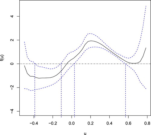
Figure 2. Relationship of treatment effect with MMSE score and Age: the estimated curve represented by real line and the corresponding 95% pointwise confidence interval by dashed line.

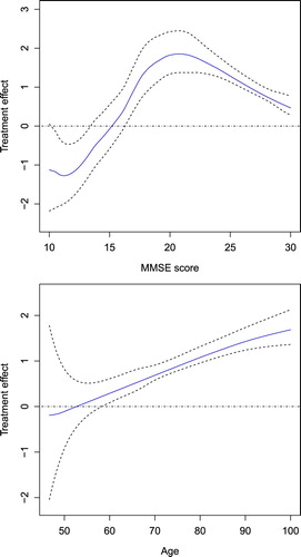
Table 5. Estimated $\alpha \alpha$ and $\text{β}\text{β}$.

Estimated $\alpha \alpha$	Estimate	Sd
Intercept	6.450	2.754
Visit year	0.029	0.026
Age	0.029	0.019
EDUC	−0.012	0.037
DIABETES	0.062	0.416
DEP	0.454	0.179
MMSE	−0.384	0.095
Estimated $\text{β}\text{β}$	Estimate	Sd
MMSE	0.842	0.115
Age	−0.540	0.304

Chen and Zhou (2011) used a generalised linear model to investigate risk factors that influence the occurrence of AD. From their results, age, DEP and MMSE score are significant under four estimation methods. They found that age and DEP have positive associations with the occurence of AD, and MMSE score is negatively correlated with the development of AD. From Table 5, our result of parametric estimates is consistent with these findings. From Figure 1, we can clearly see that if the estimated index of a patient is between 0.03 and 0.57, family inheritance of congnitive impairment increases the risk of getting AD. However, if the estimated index is between −0.39 and −0.11, family heredity decreases the risk of AD. Figure 2 shows that the effect of family heredity on occurence of AD has a bell shape association with MMSE score, that is, heredity has lower or even negative influence on risk of AD when the value of MMSE score is small or large. Also, the effect has an increasing trend with age. The effect of family heredity on occurrence of AD is stronger for elderly people.

7. Discussion

This paper focuses on a generalised partially linear single-index mixed effects model for personalised treatment effect estimation and treatment selection in longitudinal studies. In our model, the treatment effect is described as a function of a linear combination of covariates. We develop a method combining local linear regression and penalised quasi-likelihood to estimate the coefficients for each covariate, the treatment effect curve and the parameters for mixed effects. Based on the pointwise confidence intervals for treatment effect curve, we can make individualised treatment decisions from the information of patient characteristics. Our simulation study and real data analysis illustrate effectiveness of the proposed method.

Nonparametric and semiparametric methods provide a flexible way to explore HTE. The previous research in this area mostly focus on cross-sectional data. Our work fills in the gap of semiparametric modelling of HTE with longitudinal data. On the other hand, we develop a new estimation method combining local linear technique and penalised quasi-likelihood, for generalised partially linear single-index model. Pointwise confidence interval can be directly constructed for the estimated treatment effect curve based on its asymptotic normality. The theory of simultaneous confidence band for treatment effect curve can also be established accordingly, and we leave this for future work.

There are still some limitations in our work. We directly apply the method of Zhang and Peng (2010) to estimate bias and variance for the treatment effect curve. It would be more rigorous that the performance of this method in our context be validated via simulation studies. We will include this in our future research. Another limitation of our work is that, based on the pointwise confidence interval of treatment effect curve, we could only make treatment decision for a future patient. To identify subgroup of patients that benefit from each treatment, it is necessary to construct simultaneous confidence band for treatment effect curve. Some possible extensions of our work could also be considered in future research. Our model could be extended to high-dimensional covariates to cope with longitudinal studies in which large number of patient characteristics are recorded. It is also of interest to consider robust regression to limit the impact of outlying observations. An even further extension is a survival model for time-to-event response.

Acknowledgments

We are grateful to the Editor-in-Chief, Prof. Jun Shao, an Associate Editor and anonymous reviewers for their thorough reading of our manuscript and insightful comments that have led to significant improvement of this work. We also thank the US National Alzheimer's Coordinating Center for providing the data.

Disclosure statement

No potential conflict of interest was reported by the author(s).

Additional information

Funding

This work was supported by Natural Science Foundation of Shanghai (17ZR1409000). The NACC database is funded by NIA/NIH Grant U01 AG016976. NACC data are contributed by the NIA-funded ADCs: P30 AG019610 (PI Eric Reiman, MD), P30 AG013846 (PI Neil Kowall, MD), P30 AG062428-01 (PI James Leverenz, MD) P50 AG008702 (PI Scott Small, MD), P50 AG025688 (PI Allan Levey, MD, PhD), P50 AG047266 (PI Todd Golde, MD, PhD), P30 AG010133 (PI Andrew Saykin, PsyD), P50 AG005146 (PI Marilyn Albert, PhD), P30 AG062421-01 (PI Bradley Hyman, MD, PhD), P30 AG062422-01 (PI Ronald Petersen, MD, PhD), P50 AG005138 (PI Mary Sano, PhD), P30 AG008051 (PI Thomas Wisniewski, MD), P30 AG013854 (PI Robert Vassar, PhD), P30 AG008017 (PI Jeffrey Kaye, MD), P30 AG010161 (PI David Bennett, MD), P50 AG047366 (PI Victor Henderson, MD, MS), P30 AG010129 (PI Charles DeCarli, MD), P50 AG016573 (PI Frank LaFerla, PhD), P30 AG062429-01 (PI James Brewer, MD, PhD), P50 AG023501 (PI Bruce Miller, MD), P30 AG035982 (PI Russell Swerdlow, MD), P30 AG028383 (PI Linda Van Eldik, PhD), P30 AG053760 (PI Henry Paulson, MD, PhD), P30 AG010124 (PI John Trojanowski, MD, PhD), P50 AG005133 (PI Oscar Lopez, MD), P50 AG005142 (PI Helena Chui, MD), P30 AG012300 (PI Roger Rosenberg, MD), P30 AG049638 (PI Suzanne Craft, PhD), P50 AG005136 (PI Thomas Grabowski, MD), P30 AG062715-01 (PI Sanjay Asthana, MD, FRCP), P50 AG005681 (PI John Morris, MD), P50 AG047270 (PI Stephen Strittmatter, MD, PhD).

Notes on contributors

Yanghui Liu

Yanghui Liu is a Ph.D. candidate in Statistics at East China Normal University.

Riquan Zhang

Riquan Zhang is a Professor in School of Statistics at East China Normal University.

Shujie Ma

Shujie Ma is an Associate Professor in Department of Statistics at University of California, Riverside.

Xiuzhen Zhang

Xiuzhen Zhang is a Ph.D. candidate in Statistics at East China Normal University.

Appendix

Proof of Theorem 3.1.

Proof of Theorem 3.1

We use a similar proof strategy with Xu and Zhu (2012). Our proof is divided to three steps.

Step 1: Given $({\alpha \alpha }_0,{\text{β}\text{β}}_0)$, we derive the asymptotic expansion of $\hat{f}\left(u\right)-f\left(u\right)$.

Let $c_n=(Nh{)}^{-1/2},{\delta }_n=c_n^2{\log }^{1/2}(1/h)$, $\begin{array}{rl}\mathrm{\Lambda }& =\left(\begin{array}{c}{c}_n^{-1}\{a-f(u\left)\right\}\\ c_n^{-1}h\{b-f^{\mathrm{\prime }}(u\left)\right\}\end{array}\right),{FF}_{ij}=\left(\begin{array}{c}{D}_{ij}\\ h^{-1}({\text{β}\text{β}}^{\mathrm{T}}{\mathbf{Z}}_{ij}-u)D_{ij}\end{array}\right),\\ \hat{\mathrm{\Lambda }}& =\left(\begin{array}{c}{c}_n^{-1}\left\{\hat{f}\right(u)-f(u\left)\right\}\\ c_n^{-1}h\left\{{\hat{f}}^{\mathrm{\prime }}\right(u)-f(u\left)\right\}\end{array}\right).\end{array}$ Denote ${\overline{\eta }}_{ij}={\alpha \alpha }^{\mathrm{T}}{X}_{ij}+\left\{f\right(u)+f^{\mathrm{\prime }}(u\left)\right({\text{β}\text{β}}^{\mathrm{T}}{Z}_{ij}-u\left)\right\}{D}_{ij}+A_{ij}^{\mathrm{T}}{\widehat{\gamma \gamma }}_i$. By (4(4) $\begin{array}{rl}& -\frac{1}{2}\sum _{i=1}^n\left\{\sum _{j=1}^{n_i}{K}_h({\text{β}\text{β}}^{\mathrm{T}}{Z}_{ij}-u)w_{ij}{\phi }^{-1}\mathrm{d}(Y_{ij},g^{-1}[{\alpha \alpha }^{\mathrm{T}}{X}_{ij}\right.\\ & \left.\phantom{\sum _{j=1}^{n_i}}+\{a+b({\text{β}\text{β}}^{\mathrm{T}}{Z}_{ij}-u\left)\right\}{D}_{ij}+A_{ij}^{\mathrm{T}}{\gamma \gamma }_i])+{\gamma \gamma }_i^{\mathrm{T}}{GG}^{-1}{\gamma \gamma }_i\right\}\end{array}$(4) ), $\hat{\mathrm{\Lambda }}$ minimises $\begin{array}{rl}L\left(\mathrm{\Lambda }\right)& =h\sum _{i=1}^n\sum _{j=1}^{n_i}{K}_h({\text{β}\text{β}}^{\mathrm{T}}{Z}_{ij}-u)\\ & \times \left[d\{Y_{ij},g^{-1}({\overline{\eta }}_{ij}+c_n{FF}_{ij}^{\mathrm{T}}\mathrm{\Lambda }\left)\right\}-d\{Y_{ij},g^{-1}({\overline{\eta }}_{ij}\left)\right\}\right]\end{array}$ with respect to Λ. Using Taylor expansion, $\begin{array}{rl}& -\frac{1}{2}L\left(\mathrm{\Lambda }\right)\\ & =c_{n}h\sum _{i=1}^n\sum _{j=1}^{n_i}{K}_h({\text{β}\text{β}}^{\mathrm{T}}{Z}_{ij}-u)q_1({\overline{\eta }}_{ij},Y_{ij}){FF}_{ij}^{\mathrm{T}}\mathrm{\Lambda }\\ & +c_n^{2}h{\mathrm{\Lambda }}^{\mathrm{T}}\left\{\sum _{i=1}^n\sum _{j=1}^{n_i}{K}_h({\text{β}\text{β}}^{\mathrm{T}}{Z}_{ij}-u)q_2({\overline{\eta }}_{ij},Y_{ij}){FF}_{ij}{FF}_{ij}^{\mathrm{T}}\right\}\\ & \times \mathrm{\Lambda }\{1+o_p(1\left)\right\}\\ & \triangleq {TT}_n^{\mathrm{T}}\mathrm{\Lambda }+{\mathrm{\Lambda }}^{\mathrm{T}}{WW}_n\mathrm{\Lambda }\{1+o_p(1\left)\right\}.\end{array}$ Let ${\tilde{\eta }}_{ij}={\alpha \alpha }^{\mathrm{T}}{X}_{ij}+\left\{f\right(u)+f^{\mathrm{\prime }}(u\left)\right({\text{β}\text{β}}^{\mathrm{T}}{Z}_{ij}-u\left)\right\}{D}_{ij}+A_{ij}^{\mathrm{T}}{\gamma \gamma }_i$. Then ${\overline{\eta }}_{ij}-{\tilde{\eta }}_{ij}=A_{ij}^{\mathrm{T}}({\widehat{\gamma \gamma }}_i-{\gamma \gamma }_i)$. Using similar arguments as Section A.1 in Liang (2009), $\begin{array}{rl}{WW}_n& =h{c}_n^2\sum _{i=1}^n\sum _{j=1}^{n_i}{K}_h({\text{β}\text{β}}^{\mathrm{T}}{Z}_{ij}-u)q_2({\tilde{\eta }}_{ij},Y_{ij}){FF}_{ij}{FF}_{ij}^{\mathrm{T}}+o\left(h\right),\\ {TT}_n& =h{c}_n\sum _{i=1}^n\sum _{j=1}^{n_i}{K}_h({\text{β}\text{β}}^{\mathrm{T}}{Z}_{ij}-u)q_1({\tilde{\eta }}_{ij},Y_{ij}){FF}_{ij}+o\left(c_n^{-1}{h}^2\right).\end{array}$

It is easy to see that $q_2(t,y)=\{y-g^{-1}(t\left)\right\}{\rho }_1^{\mathrm{\prime }}\left(t\right)-{\rho }_2\left(t\right)$. Denote the first element of ${TT}_n$ by $T_n^{\left[1\right]}$. Using Taylor expansion, $\begin{array}{rl}{T}_n^{\left[1\right]}& =h{c}_n\sum _{i=1}^n\sum _{j=1}^{n_i}{K}_h({\text{β}\text{β}}^{\mathrm{T}}{Z}_{ij}-u)q_1\left({\eta }_{ij}\right)D_{ij}\\ & -h{c}_n\sum _{i=1}^n\sum _{j=1}^{n_i}{K}_h({\text{β}\text{β}}^{\mathrm{T}}{Z}_{ij}-u)q_2\left({\eta }_{ij}\right)\\ & \times ({\eta }_{ij}-{\tilde{\eta }}_{ij})D_{ij}\{1+o_p(1\left)\right\}\\ & =h{c}_n\sum _{i=1}^n\sum _{j=1}^{n_i}{K}_h({\text{β}\text{β}}^{\mathrm{T}}{Z}_{ij}-u)q_1\left({\eta }_{ij}\right)D_{ij}\\ & -\frac{1}{2}h{c}_n{f}^{\mathrm{\prime }\mathrm{\prime }}\left(u\right)\sum _{i=1}^n\sum _{j=1}^{n_i}{K}_h({\text{β}\text{β}}^{\mathrm{T}}{Z}_{ij}-u)q_2\left({\eta }_{ij}\right)\\ & \times ({\text{β}\text{β}}^{\mathrm{T}}{Z}_{ij}-u{)}^2{D}_{ij}^2\{1+o_p\left(1\right)\}\\ & =h{c}_n\sum _{i=1}^n\sum _{j=1}^{n_i}{K}_h({\text{β}\text{β}}^{\mathrm{T}}{Z}_{ij}-u)q_1({\eta }_{ij},Y_{ij})D_{ij}+\frac{1}{2}{c}_n^{-1}\\ & \times f^{\mathrm{\prime }\mathrm{\prime }}\left(u\right)h^2{\kappa }_2{f}_{\mathcal{U}}\left(u\right)\mathrm{E}\left\{{\rho }_2\right(\eta )D^2|{\text{β}\text{β}}^{\mathrm{T}}Z=u\}+O_p\left({\delta }_n\right).\end{array}$ Using similar arguments, we also have ${WW}_n=-f_{\mathcal{U}}\left(u\right)\mathrm{E}\left\{{\rho }_2\right(\eta )\mathrm{\Xi }|{\text{β}\text{β}}^{\mathrm{T}}Z=u\}+O_p(h^2+{\delta }_n),$ where $\mathrm{\Xi }=D^2\text{diag}(1,{\kappa }_2)$. By the concavity of function $L\left(\mathrm{\Lambda }\right)$, we obtain that $\hat{\mathrm{\Lambda }}=-{WW}_n^{-1}{TT}_n+o_p\left(1\right)$. Therefore, $\begin{array}{rl}\hat{f}\left(u\right)-f\left(u\right)& =\frac{1}{2}{f}^{\mathrm{\prime }\mathrm{\prime }}\left(u\right)h^2{\kappa }_2+{\left[f_{\mathcal{U}}\left(u\right)\mathrm{E}\left\{{\rho }_2\right(\eta )D^2|{\text{β}}^{\mathrm{T}}Z=u\}\right]}^{-1}\\ & \times N^{-1}\sum _{i=1}^n\sum _{j=1}^{n_i}{K}_h({\text{β}\text{β}}^{\mathrm{T}}{Z}_{ij}-u)q_1({\eta }_{ij},Y_{ij})D_{ij}\\ & +O_p\left({\delta }_n\right).\end{array}$

Step 2: Derive expression of ${\left.\frac{\mathrm{\partial }\hat{f}({\text{β}\text{β}}^{\mathrm{T}}z;\alpha \alpha ,\text{β}\text{β})}{\mathrm{\partial }\alpha \alpha }\right|}_{({\alpha \alpha }_0,{\text{β}\text{β}}_0^{\left(1\right)})}\mathrm{a}\mathrm{n}\mathrm{d}{\left.\frac{\mathrm{\partial }\hat{f}({\text{β}\text{β}}^{\mathrm{T}}z;\alpha \alpha ,\text{β}\text{β})}{\mathrm{\partial }{\text{β}\text{β}}^{\left(1\right)}}\right|}_{({\alpha \alpha }_0,{\text{β}\text{β}}_0^{\left(1\right)})}.$

From Step 1, $\hat{f}\left({\text{β}\text{β}}^{\mathrm{T}}z\right)$, ${\hat{f}}^{\mathrm{\prime }}\left({\text{β}\text{β}}^{\mathrm{T}}z\right)$ satisfy the following equation: (A1) $\begin{array}{rl}& N^{-1}\sum _{i=1}^n\sum _{j=1}^{n_i}{K}_h({\text{β}\text{β}}^{\mathrm{T}}{Z}_{ij}-{\text{β}\text{β}}^{\mathrm{T}}z)q_1\\ & \times \left[{\alpha \alpha }^{\mathrm{T}}{X}_{ij}+\{\hat{a}+\hat{b}({\text{β}\text{β}}^{\mathrm{T}}{Z}_{ij}-{\text{β}\text{β}}^{\mathrm{T}}z\left)\right\}{D}_{ij}+A_{ij}^{\mathrm{T}}{\gamma \gamma }_i,Y_{ij}\right]\\ & \times D_{ij}\{1+o_p(1\left)\right\}=0,\end{array}$(A1) where $\hat{a}=\hat{f}\left({\text{β}\text{β}}^{\mathrm{T}}z\right)$ and $\hat{b}={\hat{f}}^{\mathrm{\prime }}\left({\text{β}\text{β}}^{\mathrm{T}}z\right)$. Taking derivative with respect to $\alpha \alpha$ yields: $\begin{array}{rl}& N^{-1}\sum _{i=1}^n\sum _{j=1}^{n_i}{K}_h({\text{β}\text{β}}^{\mathrm{T}}{Z}_{ij}-{\text{β}\text{β}}^{\mathrm{T}}z)q_2\\ & \times \left[{\alpha \alpha }^{\mathrm{T}}{X}_{ij}+\{\hat{a}+\hat{b}({\text{β}\text{β}}^{\mathrm{T}}{Z}_{ij}-{\text{β}\text{β}}^{\mathrm{T}}z\left)\right\}{D}_{ij}+A_{ij}^{\mathrm{T}}{\gamma \gamma }_i,Y_{ij}\right]D_{ij}\\ & \times \left[X_{ij}+\left\{\frac{\mathrm{\partial }\hat{a}}{\mathrm{\partial }\alpha \alpha }+\frac{\mathrm{\partial }\hat{b}}{\mathrm{\partial }\alpha \alpha }({\text{β}\text{β}}^{\mathrm{T}}{Z}_{ij}-{\text{β}\text{β}}^{\mathrm{T}}z)\right\}{D}_{ij}\right]=0.\end{array}$ From this equation we obtain $\frac{\mathrm{\partial }\hat{a}}{\mathrm{\partial }\alpha \alpha }=-A_n^{-1}(B_{1n}+B_{2n}),$ with $\begin{array}{rl}{A}_n& =N^{-1}\sum _{i=1}^n\sum _{j=1}^{n_i}{K}_h({\text{β}\text{β}}^{\mathrm{T}}{Z}_{ij}-{\text{β}\text{β}}^{\mathrm{T}}z)q_2\\ & \times \left[{\alpha \alpha }^{\mathrm{T}}{X}_{ij}+\{\hat{a}+\hat{b}({\text{β}\text{β}}^{\mathrm{T}}{Z}_{ij}-{\text{β}\text{β}}^{\mathrm{T}}z\left)\right\}{D}_{ij}+A_{ij}^{\mathrm{T}}{\gamma \gamma }_i,Y_{ij}\right]D_{ij}^2,\\ B_{1n}& =N^{-1}\sum _{i=1}^n\sum _{j=1}^{n_i}{K}_h({\text{β}\text{β}}^{\mathrm{T}}{Z}_{ij}-{\text{β}\text{β}}^{\mathrm{T}}z)q_2\\ & \times \left[{\alpha \alpha }^{\mathrm{T}}{X}_{ij}+\{\hat{a}+\hat{b}({\text{β}\text{β}}^{\mathrm{T}}{Z}_{ij}-{\text{β}\text{β}}^{\mathrm{T}}z\left)\right\}{D}_{ij}+A_{ij}^{\mathrm{T}}{\gamma \gamma }_i,Y_{ij}\right]\\ & \times D_{ij}{X}_{ij},\\ B_{2n}& =N^{-1}\sum _{i=1}^n\sum _{j=1}^{n_i}{K}_h({\text{β}\text{β}}^{\mathrm{T}}{Z}_{ij}-{\text{β}\text{β}}^{\mathrm{T}}z)q_2\\ & \times \left[{\alpha \alpha }^{\mathrm{T}}{X}_{ij}+\{\hat{a}+\hat{b}({\text{β}\text{β}}^{\mathrm{T}}{Z}_{ij}-{\text{β}\text{β}}^{\mathrm{T}}z\left)\right\}{D}_{ij}+A_{ij}^{\mathrm{T}}{\gamma \gamma }_i,Y_{ij}\right]D_{ij}^2\\ & \times ({\text{β}\text{β}}^{\mathrm{T}}{Z}_{ij}-{\text{β}\text{β}}^{\mathrm{T}}z)\frac{\mathrm{\partial }\hat{b}}{\mathrm{\partial }\alpha \alpha }.\end{array}$ Taking derivative on (A1(A1) $\begin{array}{rl}& N^{-1}\sum _{i=1}^n\sum _{j=1}^{n_i}{K}_h({\text{β}\text{β}}^{\mathrm{T}}{Z}_{ij}-{\text{β}\text{β}}^{\mathrm{T}}z)q_1\\ & \times \left[{\alpha \alpha }^{\mathrm{T}}{X}_{ij}+\{\hat{a}+\hat{b}({\text{β}\text{β}}^{\mathrm{T}}{Z}_{ij}-{\text{β}\text{β}}^{\mathrm{T}}z\left)\right\}{D}_{ij}+A_{ij}^{\mathrm{T}}{\gamma \gamma }_i,Y_{ij}\right]\\ & \times D_{ij}\{1+o_p(1\left)\right\}=0,\end{array}$(A1) ) with respect to ${\text{β}\text{β}}^{\left(1\right)}$, we get $\begin{array}{rl}& N^{-1}\sum _{i=1}^n\sum _{j=1}^{n_i}{h}^{-1}{K}_h^{\mathrm{\prime }}({\text{β}\text{β}}^{\mathrm{T}}{Z}_{ij}-{\text{β}\text{β}}^{\mathrm{T}}z){JJ}^{\mathrm{T}}(Z_{ij}-z)q_1\\ & \times \left[{\alpha \alpha }^{\mathrm{T}}{X}_{ij}+\{\hat{a}+\hat{b}({\text{β}\text{β}}^{\mathrm{T}}{Z}_{ij}-{\text{β}\text{β}}^{\mathrm{T}}z\left)\right\}{D}_{ij}+A_{ij}^{\mathrm{T}}{\gamma \gamma }_i,Y_{ij}\right]D_{ij}\\ & +\sum _{i=1}^n\sum _{j=1}^{n_i}{K}_h({\text{β}\text{β}}^{\mathrm{T}}{Z}_{ij}-{\text{β}\text{β}}^{\mathrm{T}}z)q_2\\ & \times \left[{\alpha \alpha }^{\mathrm{T}}{X}_{ij}+\{\hat{a}+\hat{b}({\text{β}\text{β}}^{\mathrm{T}}{Z}_{ij}-{\text{β}\text{β}}^{\mathrm{T}}z\left)\right\}+A_{ij}^{\mathrm{T}}{\gamma \gamma }_i,Y_{ij}\right]D_{ij}^2\\ & \times \left\{\frac{\mathrm{\partial }\hat{a}}{\mathrm{\partial }{\text{β}\text{β}}^{\left(1\right)}}+\frac{\mathrm{\partial }\hat{b}}{\mathrm{\partial }{\text{β}\text{β}}^{\left(1\right)}}({\text{β}\text{β}}^{\mathrm{T}}{Z}_{ij}-{\text{β}\text{β}}^{\mathrm{T}}z)+\hat{b}{JJ}^{\mathrm{T}}(Z_{ij}-z)\right\}=0.\end{array}$ It follows that $\frac{\mathrm{\partial }\hat{a}}{\mathrm{\partial }{\text{β}\text{β}}^{\left(1\right)}}=-A_n^{-1}(C_{1n}+C_{2n}+C_{3n}),$ where $\begin{array}{rl}{C}_{1n}& =N^{-1}\sum _{i=1}^n\sum _{j=1}^{n_i}{K}_h({\text{β}\text{β}}^{\mathrm{T}}{Z}_{ij}-{\text{β}\text{β}}^{\mathrm{T}}z)q_2\\ & \times \left[{\alpha \alpha }^{\mathrm{T}}{X}_{ij}+\{\hat{a}+\hat{b}({\text{β}\text{β}}^{\mathrm{T}}{Z}_{ij}-{\text{β}\text{β}}^{\mathrm{T}}z\left)\right\}{D}_{ij}+A_{ij}^{\mathrm{T}}{\gamma \gamma }_i,Y_{ij}\right]\\ & \times D_{ij}^2\hat{b}{JJ}^{\mathrm{T}}(Z_{ij}-z),\\ C_{2n}& =N^{-1}\sum _{i=1}^n\sum _{j=1}^{n_i}{K}_h({\text{β}\text{β}}^{\mathrm{T}}{Z}_{ij}-{\text{β}\text{β}}^{\mathrm{T}}z)q_2\\ & \times \left[{\alpha \alpha }^{\mathrm{T}}{X}_{ij}+\{\hat{a}+\hat{b}({\text{β}\text{β}}^{\mathrm{T}}{Z}_{ij}-{\text{β}\text{β}}^{\mathrm{T}}z\left)\right\}{D}_{ij}+A_{ij}^{\mathrm{T}}{\gamma \gamma }_i,Y_{ij}\right]\\ & \times D_{ij}^2,({\text{β}\text{β}}^{\mathrm{T}}{Z}_{ij}-{\text{β}\text{β}}^{\mathrm{T}}z)\frac{\mathrm{\partial }\hat{b}}{\mathrm{\partial }{\text{β}\text{β}}^{\left(1\right)}},\\ C_{3n}& =N^{-1}\sum _{i=1}^n\sum _{j=1}^{n_i}{h}^{-1}{K}_h^{\mathrm{\prime }}({\text{β}\text{β}}^{\mathrm{T}}{Z}_{ij}-{\text{β}\text{β}}^{\mathrm{T}}z){JJ}^{\mathrm{T}}(Z_{ij}-z)q_1\\ & \times \left[{\alpha \alpha }^{\mathrm{T}}{Z}_{ij}+\{\hat{a}+\hat{b}({\text{β}\text{β}}^{\mathrm{T}}{Z}_{ij}-{\text{β}\text{β}}^{\mathrm{T}}z\left)\right\}{D}_{ij}+A_{ij}^{\mathrm{T}}{\gamma \gamma }_i,Y_{ij}\right]\\ & \times D_{ij}.\end{array}$

By similar calculations with Cui et al. (2011), $\begin{array}{rl}{A}_n& =-f_{\mathcal{U}}\left({\text{β}\text{β}}^{\mathrm{T}}z\right)\mathrm{E}\left\{{\rho }_2\left(\eta \right)D^2|{\text{β}\text{β}}^{\mathrm{T}}Z={\text{β}\text{β}}^{\mathrm{T}}z\right\}\\ & +O_p(h^2+n^{-/2}{h}^{-1/2}),\\ B_{1n}& =-f_{\mathcal{U}}\left({\text{β}\text{β}}^{\mathrm{T}}z\right)\mathrm{E}\left\{{\rho }_2\left(\eta \right)DX|{\text{β}\text{β}}^{\mathrm{T}}Z={\text{β}\text{β}}^{\mathrm{T}}z\right\}\\ & +O_p(h^2+n^{-1/2}{h}^{-1/2}),\\ B_{2n}& =O_p(h^2+n^{-1/2}{h}^{1/2}),\\ C_{1n}& =-f_{\mathcal{U}}\left({\text{β}\text{β}}^{\mathrm{T}}z\right)f^{\mathrm{\prime }}\left({\text{β}\text{β}}^{\mathrm{T}}z\right){JJ}^{\mathrm{T}}\left[\mathrm{E}\left\{{\rho }_2\right(\eta )D^{2}Z|{\text{β}\text{β}}^{\mathrm{T}}Z={\text{β}\text{β}}^{\mathrm{T}}z\}\right.\\ & \left.-\mathrm{E}\left\{{\rho }_2\right(\eta )D^2|{\text{β}\text{β}}^{\mathrm{T}}Z={\text{β}\text{β}}^{\mathrm{T}}z\}z\right]\\ & +O_p(h^2+n^{-1/2}{h}^{-1/2}),\\ C_{2n}& =O_p(h^2+n^{-1/2}{h}^{1/2}),\\ C_{3n}& =O_p(h^2+n^{-1/2}{h}^{-3/2}).\end{array}$ Therefore, $\begin{array}{rl}\frac{\mathrm{\partial }\hat{a}}{\mathrm{\partial }\alpha \alpha }& =-{\left[\mathrm{E}\left\{{\rho }_2\right(\eta )D^2|{\text{β}\text{β}}^{\mathrm{T}}Z={\text{β}\text{β}}^{\mathrm{T}}z\}\right]}^{-1}\\ & \times \left[\mathrm{E}\left\{{\rho }_2\right(\eta )DX|{\text{β}\text{β}}^{\mathrm{T}}Z={\text{β}\text{β}}^{\mathrm{T}}z\}\right]\\ & +O(h^2+n^{-1/2}{h}^{1/2}),\\ \frac{\mathrm{\partial }\hat{a}}{\mathrm{\partial }{\text{β}\text{β}}^{\left(1\right)}}& =f^{\mathrm{\prime }}\left({\text{β}\text{β}}^{\mathrm{T}}z\right){JJ}^{\mathrm{T}}\left(z-{\left[\mathrm{E}\left\{{\rho }_2\right(\eta )D^2|{\text{β}\text{β}}^{\mathrm{T}}Z={\text{β}\text{β}}^{\mathrm{T}}z\}\right]}^{-1}\right.\\ & \times \left.\left[\mathrm{E}\left\{{\rho }_2\right(\eta )D^{2}Z|{\text{β}\text{β}}^{\mathrm{T}}Z={\text{β}\text{β}}^{\mathrm{T}}z\}\right]\right)\\ & +O(h^2+n^{-1/2}{h}^{1/2}).\end{array}$

We further denote $\begin{array}{rl}\tilde{X}& =X-{\left[\mathrm{E}\left\{{\rho }_2\right(\eta \left)D^2|{\text{β}\text{β}}^{\mathrm{T}}Z\right\}\right]}^{-1}\left[\mathrm{E}\left\{{\rho }_2\right(\eta \left)DX|{\text{β}\text{β}}^{\mathrm{T}}Z\right\}\right],\\ \tilde{Z}& =f^{\mathrm{\prime }}\left({\text{β}\text{β}}^{\mathrm{T}}Z\right){JJ}^{\mathrm{T}}\left(Z-{\left[\mathrm{E}\left\{{\rho }_2\right(\eta \left)D^2|{\text{β}\text{β}}^{\mathrm{T}}Z\right\}\right]}^{-1}\right.\\ & \times \left.\left[\mathrm{E}\left\{{\rho }_2\right(\eta \left)D^{2}Z|{\text{β}\text{β}}^{\mathrm{T}}Z\right\}\right]\phantom{{\left[\mathrm{E}\left\{{\rho }_2\right(\eta \left)D^2|{\text{β}\text{β}}^{\mathrm{T}}Z\right\}\right]}^{-1}}\right).\end{array}$ It is easy to see that (A2) $\mathrm{E}\left\{{\rho }_2\right(\eta \left)D\tilde{X}|{\text{β}\text{β}}^{\mathrm{T}}Z\right\}=0,\mathrm{E}\left\{{\rho }_2\right(\eta \left)D^2\tilde{Z}|{\text{β}\text{β}}^{\mathrm{T}}Z\right\}=0.$(A2)

Step 3: The asymptotic normality of $\alpha \alpha$ and $\text{β}\text{β}$.

From estimating Equations (8(8) $\begin{array}{rl}& {SS}_{01}(\alpha \alpha ,{\text{β}\text{β}}^{\left(1\right)},\mathrm{\Gamma }\mathrm{\Gamma })\\ & =\sum _{i=1}^n\sum _{j=1}^{n_i}{X}_{ij}\left\{g^{\mathrm{\prime }}\right({\mu }_{ij}\left){\}}^{-1}{w}_{ij}{\phi }^{-1}{V}^{-1}\right({\mu }_{ij})\\ & \times \left[Y_{ij}-g^{-1}\{{\alpha \alpha }^{\mathrm{T}}{X}_{ij}+f({\text{β}\text{β}}^{\mathrm{T}}{Z}_{ij})D_{ij}+A_{ij}^{\mathrm{T}}{\gamma \gamma }_i\}\right]\\ & =00,\end{array}$(8) ) and (9(9) $\begin{array}{rl}& {SS}_{02}(\alpha \alpha ,{\text{β}\text{β}}^{\left(1\right)},\mathrm{\Gamma }\mathrm{\Gamma })\\ & =\sum _{i=1}^n\sum _{j=1}^{n_i}{JJ}_{{\text{β}\text{β}}^{\left(1\right)}}^{\mathrm{T}}{Z}_{ij}{D}_{ij}{f}^{\mathrm{\prime }}\left({\text{β}\text{β}}^{\mathrm{T}}{Z}_{ij}\right)\left\{g^{\mathrm{\prime }}\right({\mu }_{ij}){\}}^{-1}{w}_{ij}{\phi }^{-1}\\ & +V^{-1}\left({\mu }_{ij}\right)\left[Y_{ij}-g^{-1}\left\{{\alpha \alpha }^{\mathrm{T}}{X}_{ij}f\right({\text{β}\text{β}}^{\mathrm{T}}{Z}_{ij})D_{ij}+A_{ij}^{\mathrm{T}}{\gamma \gamma }_i\}\right]\\ & =00,\end{array}$(9) ), $\sqrt{N}\left(\begin{array}{c}\widehat{\alpha \alpha }-{\alpha \alpha }_0\\ {\widehat{\text{β}\text{β}}}^{\left(1\right)}-{\text{β}\text{β}}_0^{\left(1\right)}\end{array}\right)={\mathcal{A}}_n^{-1}\sqrt{N}{\mathcal{B}}_n+o_p\left(1\right),$ where $\begin{array}{rl}{\mathcal{A}}_n& =\frac{1}{N}\sum _{i=1}^n\sum _{j=1}^{n_i}{\rho }_2\left({\eta }_{ij}\right)\left(\begin{array}{c}{X}_{ij}\\ f^{\mathrm{\prime }}\left({\text{β}\text{β}}_0^{\mathrm{T}}{Z}_{ij}\right){JJ}^{\mathrm{T}}{Z}_{ij}{D}_{ij}\end{array}\right){\left(\begin{array}{c}{\tilde{X}}_{ij}\\ {\tilde{Z}}_{ij}{D}_{ij}\end{array}\right)}^{\mathrm{T}},\\ {\mathcal{B}}_n& =\frac{1}{N}\sum _{i=1}^n\sum _{j=1}^{n_i}\left(\begin{array}{c}{X}_{ij}\\ f^{\mathrm{\prime }}\left({\text{β}\text{β}}_0^{\mathrm{T}}{Z}_{ij}\right){JJ}^{\mathrm{T}}{Z}_{ij}{D}_{ij}\end{array}\right)\left\{g^{\mathrm{\prime }}\right({\mu }_{ij}\left){\}}^{-1}{V}^{-1}\right({\mu }_{ij})\\ & \times \left[Y_{ij}-g^{-1}\{{\alpha \alpha }_0^{\mathrm{T}}{X}_{ij}+\hat{f}({\text{β}\text{β}}_0^{\mathrm{T}}{Z}_{ij})D_{ij}+A_{ij}^{\mathrm{T}}{\gamma \gamma }_i\right].\end{array}$

Based on (A2(A2) $\mathrm{E}\left\{{\rho }_2\right(\eta \left)D\tilde{X}|{\text{β}\text{β}}^{\mathrm{T}}Z\right\}=0,\mathrm{E}\left\{{\rho }_2\right(\eta \left)D^2\tilde{Z}|{\text{β}\text{β}}^{\mathrm{T}}Z\right\}=0.$(A2) ), we have ${\mathcal{A}}_n=\mathrm{E}\left({\rho }_2\left(\eta \right){\left(\begin{array}{c}\tilde{X}\\ \tilde{Z}D\end{array}\right)}^{\otimes 2}\right)+o_p\left(1\right)\triangleq \mathcal{A}+o_p\left(1\right).$ By Taylor expansion, ${\mathcal{B}}_n={\mathcal{B}}_{1n}+{\mathcal{B}}_{2n}\{1+o_p(1\left)\right\},$ where $\begin{array}{rl}{\mathcal{B}}_{1n}& =\frac{1}{N}\sum _{i=1}^n\sum _{j=1}^{n_i}\left(\begin{array}{c}{X}_{ij}\\ f^{\mathrm{\prime }}\left({\text{β}\text{β}}_0^{\mathrm{T}}{Z}_{ij}\right){JJ}^{\mathrm{T}}{Z}_{ij}{D}_{ij}\end{array}\right)q_1({\eta }_{ij},Y_{ij}),\\ {\mathcal{B}}_{2n}& =-\frac{1}{N}\sum _{i=1}^n\sum _{j=1}^{n_i}\left(\begin{array}{c}{X}_{ij}\\ f^{\mathrm{\prime }}\left({\text{β}\text{β}}_0^{\mathrm{T}}{Z}_{ij}\right){JJ}^{\mathrm{T}}{Z}_{ij}{D}_{ij}\end{array}\right){\rho }_2\left({\eta }_{ij}\right)\left\{\hat{f}\right({\text{β}\text{β}}_0^{\mathrm{T}}{Z}_{ij})\\ & -f\left({\text{β}\text{β}}_0^{\mathrm{T}}{Z}_{ij}\right)\}{D}_{ij}.\end{array}$ From the result of Step 1, $\begin{array}{rl}\sqrt{N}{\mathcal{B}}_{2n}& =-\frac{1}{\sqrt{N}}\sum _{i=1}^n\sum _{j=1}^{n_i}\left(\begin{array}{c}{X}_{ij}\\ f^{\mathrm{\prime }}\left({\text{β}\text{β}}_0^{\mathrm{T}}{Z}_{ij}\right){JJ}^{\mathrm{T}}{Z}_{ij}{D}_{ij}\end{array}\right){\rho }_2\left({\eta }_{ij}\right)D_{ij}\\ & \times {\left[f_{\mathcal{U}}\left({\text{β}\text{β}}_0^{\mathrm{T}}{Z}_{ij}\right)\mathrm{E}\left\{{\rho }_2\right(\eta )D^2|{\text{β}\text{β}}_0^{\mathrm{T}}Z={\text{β}\text{β}}_0^{\mathrm{T}}{Z}_{ij}\}\right]}^{-1}\\ & \times \frac{1}{N}\sum _{k=1}^n\sum _{l=1}^{n_i}{K}_h({\text{β}\text{β}}_0^{\mathrm{T}}{Z}_{kl}-{\text{β}\text{β}}_0^{\mathrm{T}}{Z}_{ij})q_1({\eta }_{kl},Y_{kl})D_{kl}\\ & -\frac{1}{2}{h}^2{\kappa }_2\frac{1}{\sqrt{N}}\sum _{i=1}^n\sum _{j=1}^{n_i}\left(\begin{array}{c}{X}_{ij}\\ f^{\mathrm{\prime }}\left({\text{β}\text{β}}_0^{\mathrm{T}}{Z}_{ij}\right){JJ}^{\mathrm{T}}{Z}_{ij}{D}_{ij}\end{array}\right)\\ & \times {\rho }_2\left({\eta }_{ij}\right)D_{ij}{f}^{\mathrm{\prime }\mathrm{\prime }}\left({\text{β}\text{β}}^{\mathrm{T}}{Z}_{ij}\right)\\ & =-\frac{1}{\sqrt{N}}\sum _{k=1}^n\sum _{l=1}^{n_i}{q}_1({\eta }_{kl},Y_{kl})D_{kl}\\ & \times \sum _{i=1}^n\sum _{j=1}^{n_i}{K}_h({\text{β}\text{β}}_0^{\mathrm{T}}{Z}_{ij}-{\text{β}\text{β}}_0^{\mathrm{T}}{Z}_{kl})\\ & \times \left(\begin{array}{c}{X}_{ij}\\ f^{\mathrm{\prime }}\left({\text{β}\text{β}}_0^{\mathrm{T}}{Z}_{ij}\right){JJ}^{\mathrm{T}}{Z}_{ij}{D}_{ij}\end{array}\right){\rho }_2\left({\eta }_{ij}\right)D_{ij}\\ & \times {\left[f_{\mathcal{U}}\left({\text{β}\text{β}}_0^{\mathrm{T}}{Z}_{ij}\right)\mathrm{E}\left\{{\rho }_2\right(\eta )D^2|{\text{β}\text{β}}_0^{\mathrm{T}}Z={\text{β}\text{β}}_0^{\mathrm{T}}{Z}_{ij}\}\right]}^{-1}\\ & +O_p\left(n^{1/2}{h}^2\right)\\ & =-\frac{1}{\sqrt{N}}\sum _{i=1}^n\sum _{j=1}^{n_i}{\left[\mathrm{E}\left\{{\rho }_2\right(\eta )D^2|{\text{β}\text{β}}_0^{\mathrm{T}}Z={\text{β}\text{β}}_0^{\mathrm{T}}{Z}_{ij}\}\right]}^{-1}\\ & \times \left[\begin{array}{c}\mathrm{E}\left\{{\rho }_2\left(\eta \right)DX|{\text{β}\text{β}}_0^{\mathrm{T}}Z={\text{β}\text{β}}_0^{\mathrm{T}}{Z}_{ij}\right\}\\ f^{\mathrm{\prime }}\left({\text{β}\text{β}}_0^{\mathrm{T}}{Z}_{ij}\right){JJ}^{\mathrm{T}}\mathrm{E}\left\{{\rho }_2\right(\eta )D^{2}Z|{\text{β}\text{β}}_0^{\mathrm{T}}Z={\text{β}\text{β}}_0^{\mathrm{T}}{Z}_{ij}\}\end{array}\right]\\ & \times D_{ij}{q}_1({\eta }_{ij},Y_{ij})+o_p\left(1\right).\end{array}$ It is easy to see that $\sqrt{N}{\mathcal{B}}_n=\frac{1}{\sqrt{N}}\sum _{i=1}^n\sum _{j=1}^{n_i}\left(\begin{array}{c}{\tilde{X}}_{ij}\\ {\tilde{Z}}_{ij}{D}_{ij}\end{array}\right)q_1({\eta }_{ij},Y_{ij}).$ By CLT, $\sqrt{N}{\mathcal{B}}_n$ has asymptotic normal distribution with zero-mean. Denote $s_{ij}=\left(\begin{array}{c}{\tilde{X}}_{ij}\\ {\tilde{Z}}_{ij}{D}_{ij}\end{array}\right)$, we have $\begin{array}{rl}\mathrm{v}\mathrm{a}\mathrm{r}\left(\sqrt{N}{\mathcal{B}}_n\right)& =\frac{1}{N}\sum _{i=1}^n\sum _{j=1}^{n_i}\mathrm{v}\mathrm{a}\mathrm{r}\left\{s_{ij}{q}_1\right({\eta }_{ij},Y_{ij}\left)\right\}\\ & +\frac{1}{N}\sum _{i=1}^n\sum _{j=1}^{n_i}\sum _{\begin{array}{c}k=1\\ k\ne j\end{array}}^{n_i}\text{cov}\left\{s_{ij}{q}_1\right({\eta }_{ij},Y_{ij}),\\ & s_{ik}{q}_1({\eta }_{ik},Y_{ik})\}.\end{array}$ Using simple calculation, $\mathrm{v}\mathrm{a}\mathrm{r}\left\{s_{ij}{q}_1\right({\eta }_{ij},Y_{ij}\left)\right\}=\mathrm{E}\left\{{\rho }_2\right(\eta \left)s{s}^{\mathrm{T}}\right\}=\mathcal{A}.$ Denote $\mathcal{C}=\text{cov}\left\{s_{11}{q}_1\right({\eta }_{11},Y_{11}),s_{12}{q}_1({\eta }_{12},Y_{12}\left)\right\}$, $\mathrm{v}\mathrm{a}\mathrm{r}\left(\sqrt{N}{\mathcal{B}}_n\right)=\mathcal{A}+\frac{N_1}{N}\mathcal{C}.$Therefore, when $n\to \mathrm{\infty }$, $\sqrt{N}\left(\begin{array}{c}\widehat{\alpha \alpha }-{\alpha }_0\\ {\widehat{\text{β}\text{β}}}^{\left(1\right)}-{\text{β}\text{β}}_0^{\left(1\right)}\end{array}\right)\to N(0,{\mathcal{A}}^{-1}+\frac{N_1}{N}{\mathcal{A}}^{-1}\mathcal{C}{\mathcal{A}}^{-1}).$

Denote $\mathcal{D}=\left(\begin{array}{cc}{II}_p& {00}_{p\times (q-1)}\\ {00}_{q\times p}& {JJ}_{{\text{β}\text{β}}_0^{\left(1\right)}}\end{array}\right)$. An application of multivariate delta-method yields $\sqrt{N}\left(\begin{array}{c}\widehat{\alpha \alpha }-{\alpha }_0\\ \widehat{\text{β}\text{β}}-{\text{β}\text{β}}_0\end{array}\right)\to N(0,\mathrm{\Sigma }\mathrm{\Sigma }),$ where $\mathrm{\Sigma }\mathrm{\Sigma }=\mathcal{D}({\mathcal{A}}^{-1}+\frac{N_1}{N}{\mathcal{A}}^{-1}\mathcal{C}{\mathcal{A}}^{-1}){\mathcal{D}}^{\mathrm{T}}$.

Proof of Theorem 3.2

Proof of Theorem 3.2

From Theorem 3.1, $\sqrt{N}\left(\begin{array}{c}\widehat{\alpha \alpha }-{\alpha \alpha }_0\\ {\widehat{\text{β}\text{β}}}^{\left(1\right)}-{\text{β}\text{β}}_0^{\left(1\right)}\end{array}\right)=O_p\left(1\right)$. We write $\begin{array}{rl}& \hat{f}({\widehat{\text{β}\text{β}}}^{\mathrm{T}}z;\widehat{\alpha \alpha },\widehat{\text{β}\text{β}})-f\left({\text{β}\text{β}}_0^{\mathrm{T}}z\right)\\ & =\hat{f}({\widehat{\text{β}\text{β}}}^{\mathrm{T}}z;\widehat{\alpha \alpha },\widehat{\text{β}\text{β}})-\hat{f}\left({\text{β}\text{β}}_0^{\mathrm{T}}z\right)+\hat{f}\left({\text{β}\text{β}}_0^{\mathrm{T}}z\right)-f\left({\text{β}\text{β}}_0^{\mathrm{T}}z\right)\\ & =\frac{\mathrm{\partial }\hat{f}({\text{β}\text{β}}^{\mathrm{T}}z;\alpha \alpha ,\text{β}\text{β})}{\mathrm{\partial }({\alpha \alpha }^{\mathrm{T}},{\text{β}\text{β}}^{\left(1\right)\mathrm{T}})}{|}_{({\alpha \alpha }_0,{\text{β}\text{β}}_0^{\left(1\right)})}\left(\begin{array}{c}\widehat{\alpha \alpha }-{\alpha \alpha }_0\\ {\widehat{\text{β}\text{β}}}^{\left(1\right)}-{\text{β}\text{β}}_0^{\left(1\right)}\end{array}\right)\{1+o_p(1\left)\right\}\\ & +\left\{\hat{f}\left({\text{β}\text{β}}_0^{\mathrm{T}}z\right)-f\left({\text{β}\text{β}}_0^{\mathrm{T}}z\right)\right\}\\ & =\hat{f}\left({\text{β}\text{β}}_0^{\mathrm{T}}z\right)-f\left({\text{β}\text{β}}_0^{\mathrm{T}}z\right)+O_p\left(n^{-1/2}\right).\end{array}$ Hence the asymptotic distribution of $\hat{f}({\widehat{\text{β}\text{β}}}^{\mathrm{T}}z;\widehat{\alpha \alpha },\widehat{\text{β}\text{β}})$ is the same as that of $\hat{f}\left({\text{β}\text{β}}_0^{\mathrm{T}}z\right)$. Based on the result of Step 1, we now derive the asymptotic variance of $\hat{f}\left({\text{β}\text{β}}_0^{\mathrm{T}}z\right)$. Denote $r_{ij}=K_h({\text{β}\text{β}}_0^{\mathrm{T}}{Z}_{ij}-{\text{β}\text{β}}_0^{\mathrm{T}}z)q_1({\eta }_{ij},Y_{ij})D_{ij}$, we have $\begin{array}{rl}\mathrm{v}\mathrm{a}\mathrm{r}\left\{\sum _{i=1}^n\sum _{j=1}^{n_i}{r}_{ij}\right\}& =\sum _{i=1}^n\sum _{j=1}^{n_i}\mathrm{v}\mathrm{a}\mathrm{r}\left(r_{ij}\right)\\ & +\sum _{i=1}^n\sum _{j=1}^{n_i}\sum _{\begin{array}{c}k=1\\ k\ne j\end{array}}^{n_i}\text{cov}(r_{ij},r_{ik}),\end{array}$ where $\begin{array}{rl}\mathrm{v}\mathrm{a}\mathrm{r}\left(r_{ij}\right)& =\mathrm{E}{K}_h^2({\text{β}\text{β}}_0^{\mathrm{T}}{Z}_{ij}-{\text{β}\text{β}}_0^{\mathrm{T}}z)q_1^2({\eta }_{ij},Y_{ij})D_{ij}^2\\ & =h^{-1}{\mu }_0{f}_{\mathcal{U}}\left({\text{β}\text{β}}_0^{\mathrm{T}}z\right)\mathrm{E}\left\{{\rho }_2\right(\eta )D^2|{\text{β}\text{β}}_0^{\mathrm{T}}Z={\text{β}\text{β}}_0^{\mathrm{T}}z\},\\ \text{cov}(r_{ij},r_{ik})& =f_{\mathcal{U}}^2\left({\text{β}\text{β}}_0^{\mathrm{T}}z\right)\mathrm{E}\left\{q_1({\eta }_{11},Y_{11})q_1({\eta }_{12},Y_{12})D_{11}^2\right.\\ & \left.D_{12}^2|{\text{β}\text{β}}_0^{\mathrm{T}}{Z}_{11}={\text{β}\text{β}}_0^{\mathrm{T}}z,{\text{β}\text{β}}_0^{\mathrm{T}}{Z}_{12}={\text{β}\text{β}}_0^{\mathrm{T}}z\right\}.\end{array}$ Therefore, we have $\sqrt{Nh}\left\{\hat{f}\right({\widehat{\text{β}\text{β}}}^{\mathrm{T}}z;\widehat{\alpha \alpha },\widehat{\text{β}\text{β}})-f({\text{β}\text{β}}_0^{\mathrm{T}}z)-\frac{1}{2}{h}^2{\kappa }_2{f}^{\mathrm{\prime }\mathrm{\prime }}({\text{β}\text{β}}_0^{\mathrm{T}}z\left)\right\}\to N(0,{\sigma }_f^2),$ where ${\sigma }_f^2={\mu }_0{f}_{\mathcal{U}}^{-1}\left({\text{β}\text{β}}_0^{\mathrm{T}}z\right)\left[\mathrm{E}\right\{{\rho }_2\left(\eta \right)D^2|{\text{β}\text{β}}_0^{\mathrm{T}}Z={\text{β}\text{β}}_0^{\mathrm{T}}z\}{]}^{-1}$.

References

- Berger, J. O., Wang, X., & Shen, L. (2014). A Bayesian approach to subgroup identification. Journal of Biopharmaceutical Statistics, 24(1), 110–129. https://doi.org/10.1080/10543406.2013.856026
- Bonetti, M., & Gelber, R. (2004). Patterns of treatment eects in subsets of patients in clinical trials. Biostatistics, 5(3), 465–481. https://doi.org/10.1093/biostatistics/kxh002
- Bonetti, M., Zahrieh, D., Cole, B. F., & Gelber, R. D. (2009). A small sample study of the stepp approach to assessing treatment-covariate interactions in survival data. Statistics in Medicine, 28(8), 1255–1268. https://doi.org/10.1002/sim.v28:8 doi: https://doi.org/10.1002/sim.3524
- Breslow, N. E., & Clayton, D. G. (1993). Approximate inference in generalized linear mixed models. Journal of the American Statistical Association, 88(21), 9–25. https://doi.org/10.1080/01621459.1993.10594284.
- Carroll, R. J., Fan, J., Gijbels, I., & Wand, M. P. (1997). Generalized partially linear single-index models. Journal of the American Statistical Association, 92(438), 477–489. https://doi.org/10.1080/01621459.1997.10474001
- Chen, J., Kim, I., Terrell, G. R., & Liu, L. (2014). Generalized partially linear single-index mixed model for repeated measures data. Journal of Nonparametric Statistics, 26(2), 291–303. https://doi.org/10.1080/10485252.2014.891029
- Chen, B., & Zhou, X. (2011). Doubly robust estimates for binary longitudinal data analysis with missing response and missing covariates. Biometrics, 67(3), 830–842. https://doi.org/10.1111/biom.2011.67.issue-3 doi: https://doi.org/10.1111/j.1541-0420.2010.01541.x
- Ciampi, A., Negassa, A., & Lou, Z. (1995). Tree-structured prediction for censored survival data and the cox model. Journal of Clinical Epidemiology, 48(5), 675–689. https://doi.org/10.1016/0895-4356(94)00164-L
- Cui, X., Härdle, W. K., & Zhu, L. (2011). The EFM approach for single-index models. The Annals of Statistics, 39(3), 1658–2688. https://projecteuclid.org/euclid.aos/1311600279 doi: https://doi.org/10.1214/10-AOS871
- Foster, J. C., Taylor, J. M. G., Kaciroti, N., & Nan, B. (2015). Simple subgroup approximations to optimal treatment regimes from randomized clinical trial data. Biostatistics, 16(2), 368–382. https://doi.org/10.1093/biostatistics/kxu049
- Foster, J. C., Taylor, J. M.G., & Ruberg, S. J. (2011). Subgroup identification from randomized clinical trial data. Statistics in Medicine, 30(24), 2867–2880. https://doi.org/10.1002/sim.v30.24 doi: https://doi.org/10.1002/sim.4322
- Guo, W., Zhou, X., & Ma, S. (2018). Optimal treatment selection using the covariate-specific treatment effect curve with high-dimensional covariates, arXiv:1812.10018.
- Han, K., Zhou, X., & Liu, B. (2017). CSTE curve for selection the optimal treatment when outcome is binary. Scientia Sinica (Mathematica), 47(4), 497–514. https://doi.org/10.1360/SCM-2015-0595
- Laird, N. M., & Ware, J. H. (1982). Random effects models for longitudinal data. Biometrics, 38(4), 963–974. https://doi.org/10.2307/2529876
- Liang, H. (2009). Generalized partially linear mixed-effects models incorporating mismeasured covariates. Annals of the Institute of Statistical Mathematics, 61(1), 27–46. https://doi.org/10.1007/s10463-007-0146-0
- Ma, Y., & Zhou, X. (2014). Treatment selection in a randomized clinical trial via covariate-specific treatment effect curves. Statistical Methods in Medical Research, 26(1), 124–141. https://doi.org/10.1177/0962280214541724
- Negassa, A., Ciampi, A., Abrahamowicz, M., Shapiro, S., & Boivin, J. (2005). Tree-structured subgroup analysis for censored survival data: validation of computationally inexpensive model selection criteria. Statistics and Computing, 15(3), 231–239. https://doi.org/10.1007/s11222-005-1311-z
- Pang, Z., & Xue, L. (2012). Estimation for the single-index models with random effects. Computational Statistics & Data Analysis, 56(6), 1837–1853. https://doi.org/10.1016/j.csda.2011.11.007
- Su, X., Tsai, C., Wang, H., Nickerson, D., & Li, B. (2008). Subgroup analysis via recursive partitioning. Journal of Machine Learning Research, 10, 141–158. https://dl.acm.org/doi/10.5555/1577069.1577074.
- Wang, R., Lagakos, S. W., Ware, J. H., Hunter, D. J., & Drazen, J. M. (2007). Statistics in medicine – Reporting of subgroup analyses in clinical trials. The New England Journal of Medicine, 357(21), 2189–2194. https://doi.org/10.1056/NEJMsr077003
- Wu, H., & Zhang, J. T. (2006). Nonparametric regression methods for longitudinal data analysis. John Wiley & Sons.
- Xu, P., & Zhu, L. X. (2012). Estimation for a marginal generalized single-index longitudinal model. Journal of Multivariate Analysis, 105(1), 285–299. https://doi.org/10.1016/j.jmva.2011.10.004
- Zhang, W., & Peng, H. (2010). Simultaneous confidence band and hypothesis test in generalised varying-coefficient models. Journal of Multivariate Analysis, 101(7), 1656–1680. https://doi.org/10.1016/j.jmva.2010.03.003