A three-parameter logistic regression model

Abstract

Dose–response experiments and data analyses are often carried out according to an optimal design under a model assumption. A two-parameter logistic model is often used because of its nice mathematical properties and plausible stochastic response mechanisms. There is an extensive literature on its optimal designs and data analysis strategies. However, a model is at best a good approximation in a real-world application, and researchers must be aware of the risk of model mis-specification. In this paper, we investigate the effectiveness of the sequential ED-design, the D-optimal design, and the up-and-down design under the three-parameter logistic regression model, and we develop a numerical method for the parameter estimation. Simulations show that the combination of the proposed model and the data analysis strategy performs well. When the logistic model is correct, this more complex model has hardly any efficiency loss. The three-parameter logistic model works better than the two-parameter logistic model in the presence of model mis-specification.

Keywords:

• dose–response experiment
• effective dose level
• optimal design
• sequential ED-design
• up-and-down design
• vertex direction method

MSC 2010:

• Primary: 62K05
• Secondary: 62L05

1. Introduction

Dose–response experiments are routinely conducted to study the relationship between the dose of a stimulus and the response of the experiment subjects. Simple and easy-to-interpret models are preferred for the dose–response relationship. The goal of the experiment is often to accurately determine the median dose level: the level of stimulant at which half the recipients respond. Other effective dose levels are also of interest.

There has been much discussion of optimal designs where the dose–response relationship is completely known (Ford et al., 1985; Sitter & Fainaru, 1997; Sitter & Forbes, 1997; Sitter & Wu, 1993; Wu, 1985). In applications, one may first run a pilot study to obtain an estimate of the dose–response relationship. The optimal design based on the fitted model is then used to guide further experiments (P. Li & Wiens, 2011; Wang et al., 2013; Wu & Tian, 2014). A full sequential approach can also be used: the parameter estimates are updated after each run, and the result is used to suggest dose levels for the subsequent runs.

Naturally, if the model is mis-specified, the optimal design is misguided and the effective dose levels can be poorly estimated. One way to reduce the risk of model mis-specification is to apply a more flexible and hence more complex dose–response model. We seek a trade-off between model flexibility and inference efficacy. A nonparametric model is the most flexible and free from the risk of model mis-specification. However, it likely needs more experiment runs to achieve the same estimation precision as an analysis under approximately valid parametric assumptions. The commonly used logistic or probit models are simple and have good mathematical and statistical properties. They are satisfactory in many applications, but their model assumptions impose restrictions on the dose–response relationship. A slightly more complex model can lower the risk of mis-specification without complicating the issues related to optimal design and data analysis (El-Saidi, 1993; G. Li & Majumdar, 2008; O'Brien et al., 2009).

In this paper, we study the design and analysis problems for a three-parameter logistic regression model. We develop an easy-to-implement iterative numerical algorithm with guaranteed convergence for the maximum likelihood estimate (MLE). We investigate the effectiveness of the sequential ED-design (Yu et al., 2016) and the D-optimal design. The ED-design optimises the estimation of targeted effective dose-levels while the D-optimal design targets model parameters. See Sections 3.3 and 3.2. We use the vertex direction method (VDM) to find the D-optimal design.

Simulation studies show that the combination of the proposed model, design, and data analysis strategy performs well. When the logistic model is correct, the three-parameter model has little efficiency loss. When the three-parameter model holds but the logistic model is violated, the new approach is more efficient.

The paper is organised as follows. In Section 2, we introduce the three-parameter logistic model and a numerical algorithm for the MLE. Design problems under this model are discussed in Section 3. In Section 4, we present some simulation results and an example. Section 5 provides concluding remarks.

2. Three-parameter logistic model and the MLE

Consider a dose–response experiment in which a stimulant at level X is applied to a subject. The subject either responds (Y = 1) or does not respond (Y = 0) to the stimulus. The dose–response relationship is defined to be $\pi \left(x\right)=P(Y=1|X=x).$ In most applications, we envisage $\pi \left(x\right)$ as a smooth increasing function of x. Based on data collected on the response values, $y_1,\dots ,y_n$, for selected dose levels, $x_1,\dots ,x_n$, scientists may be interested in the accurate estimation of a specific dose level $x=\mathrm{e}\mathrm{d}50$ at which $\pi \left(x\right)=0.5$. We use edγ to denote the effective dose level at which the probability of response is $\gamma \mathrm{\%}$. One may also focus on the shape of $\pi \left(x\right)$ for x between, for example, ed25 and ed75.

If one is interested in a single ED level, effective statistical inference is possible without a parametric assumption on $\pi \left(x\right)$. If a detailed dose–response relationship is desired over a dose range, then a suggested parametric form $\pi \left(x\right)$ is likely necessary and helpful. A commonly employed model for $\pi \left(x\right)$ is the logistic dose–response relationship: (1) $\mathrm{l}\mathrm{o}\mathrm{g}\mathrm{i}\mathrm{t}\left\{\pi \right(x\left)\right\}=\log \left\{\frac{\pi \left(x\right)}{1-\pi \left(x\right)}\right\}=\alpha +\text{β}x$(1) for parameters α and β. In applications, the dose level may be log-transformed before the logistic or other model is applied (G. Li & Majumdar, 2008; O'Brien et al., 2009). In addition to its mathematical convenience, the logistic regression model permits the interpretation of the size of β. For example, in epidemiology, when Y stands for catching a disease and x for the exposure level, the value of β is the log-odds ratio of catching the disease when the exposure level is increased by a unit.

Statisticians and scientists are keenly aware that the logistic and other two-parameter models can be poor approximations of the true dose–response relationship. A more flexible model can be advantageous if it is not too complex. One such choice is a three-parameter logistic dose–response model (El-Saidi, 1993): (2) $\mathrm{l}\mathrm{o}\mathrm{g}\mathrm{i}\mathrm{t}\left\{{\pi }^{\lambda }\right(x\left)\right\}=\log \left\{\frac{{\pi }^{\lambda }\left(x\right)}{1-{\pi }^{\lambda }\left(x\right)}\right\}=\alpha +\text{β}x.$(2) We require $\lambda >0$ to ensure that ${\pi }^{\lambda }\left(x\right)$ is between 0 and 1, and we do not place restrictions on α and β.

We note that when $\lambda =1$, the three-parameter model becomes the commonly used logistic model. In this case, for any $\gamma \in (0,100)$, the model satisfies $\mathrm{e}\mathrm{d}\gamma +\mathrm{e}\mathrm{d}(100-\gamma )=-\frac{2\alpha }{\text{β}}$ assuming $\text{β}\ne 0$. Such a restriction is hard to justify in applications. The introduction of the parameter λ helps to soften this restriction without overburdening the system. Under this model, the effective dose level at γ is given by $\mathrm{e}\mathrm{d}\gamma =\frac{\text{logit}(\left(\gamma /100{)}^{\lambda }\right)-\alpha }{\text{β}}.$ An explicit expression for the dose–response relationship is $\pi \left(x\right)=P\{Y=1|X=x\}={\left\{\frac{\exp (\alpha +\text{β}x)}{1+\exp (\alpha +\text{β}x)}\right\}}^{1/\lambda }.$ As discussed in Yu et al. (2016), many sequential designs, including the ED-design, contain a step to update the estimate of the model parameters. The MLE is a common choice.

2.1. Numerical method for MLE

Let $(x_i,y_i):i=1,\dots ,n$ be observations from a dose–response experiment and assume model (2(2) $\mathrm{l}\mathrm{o}\mathrm{g}\mathrm{i}\mathrm{t}\left\{{\pi }^{\lambda }\right(x\left)\right\}=\log \left\{\frac{{\pi }^{\lambda }\left(x\right)}{1-{\pi }^{\lambda }\left(x\right)}\right\}=\alpha +\text{β}x.$(2) ). The log-likelihood based on this data set is given by ${\ell }_n\left(\theta \right)=\sum _{i=1}^n\left\{y_i\log (\pi \left(x_i\right))+(1-y_i)\log (1-\pi \left(x_i\right))\right\}$ where $\theta =(\alpha ,\text{β},\lambda {)}^{\mathrm{T}}$.

When $\lambda =1$ is fixed, the model becomes the usual logistic model, and ${\ell }_n\left(\theta \right)$ is known to be concave in α and β. The concavity permits a simple numerical solution to the MLE of α and β. We remark that when the $x_i$'s corresponding to y = 1 are completely separated from those corresponding to y = 0, the maximum point $\widehat{\text{β}}=\pm \mathrm{\infty }$. This problem is easily avoided by adding informative pseudo-observations, as in Yu et al. (2016), and this is done implicitly in our calculations.

Given any value of λ, the log-likelihood is concave in α and β. Given any α and β, the log-likelihood is concave in λ. Because of these properties, the following two-loop iterative numerical algorithm works nicely. We start with the initial value ${\lambda }^{\left(0\right)}=1$ and set k = 0. Let ε be a small positive value such as ${10}^{-5}$.

1. Let ${\ell }_n^{\left(k\right)}(\alpha ,\text{β})={\ell }_n(\alpha ,\text{β},{\lambda }^{\left(k\right)})$. Use an iterative algorithm to solve $({\alpha }^{(k+1)},{\text{β}}^{(k+1)})=\underset{\alpha ,\text{β}}{\arg max}{\ell }_n^{\left(k\right)}(\alpha ,\text{β}).$

2. Let $a_i=\frac{\exp ({\alpha }^{(k+1)}+{\text{β}}^{(k+1)}{x}_i)}{1+\exp ({\alpha }^{(k+1)}+{\text{β}}^{(k+1)}{x}_i)}$ and define ${\ell }_n^{\left(k\right)}\left(\lambda \right)=\sum _{i=1}^n\left\{\right(1-y_i)\log (1-a_i^{\lambda })+y_i\log (a_i^{\lambda }\left)\right\}.$ Use an iterative algorithm to solve ${\lambda }^{(k+1)}=\arg \underset{\lambda }{max}{\ell }_n^{\left(k\right)}\left(\lambda \right).$ Write ${\theta }^{\left(k\right)}=({\alpha }^{\left(k\right)},{\text{β}}^{\left(k\right)},{\lambda }^{\left(k\right)}{)}^{\tau }$. If ${\ell }_n\left({\theta }^{(k+1)}\right)-{\ell }_n\left({\theta }^{\left(k\right)}\right)\le ϵ$, stop and report ${\theta }^{(k+1)}$ and ${\ell }_n\left({\theta }^{(k+1)}\right)$. Otherwise, set k = k + 1 and return to Step (1).

In the above presentation, we have used ${\ell }_n^{\left(k\right)}(\alpha ,\text{β})$ and ${\ell }_n^{\left(k\right)}\left(\lambda \right)$ as two different functions. The objective functions in both loops are concave, and they thus guarantee the convergence of any sensible iterative procedures that we may use in these two steps, and hence of the entire algorithm. We state the concave conclusions in two lemmas.

Lemma

Function ${\ell }_n^{\left(k\right)}\left(\lambda \right)$ in Step (2) is concave in λ given any data set $(x_i,y_i)$ for $i=1,2,\dots ,n$ with $n\ge 1$.

Proof.

To prove the concavity, it suffices to show that the second derivative of this function is always nonnegative. Straightforward algebra shows that $\frac{\mathrm{\partial }{\ell }_n^{\left(k\right)}\left(\lambda \right)}{\mathrm{\partial }\lambda }=\sum _{i=1}^n\frac{(y_i-a_i^{\lambda })(\log a_i)}{1-a_i^{\lambda }}$ and subsequently $\frac{{\mathrm{\partial }}^2{\ell }_n^{\left(k\right)}\left(\lambda \right)}{\mathrm{\partial }{\lambda }^2}=\sum _{i=1}^n\frac{a_i^{\lambda }(y_i-1)(\log a_i{)}^2}{(1-a_i^{\lambda }{)}^2}\le 0$ since $y_i\le 1$ for all i. Therefore, the function is concave as claimed.

Lemma

Given any data set $(x_i,y_i)$ for $i=1,2,\dots ,n$ with $n\ge 1$, the objective function ${\ell }_n^{\left(k\right)}(\alpha ,\text{β})$ in Step (1) is concave in $\alpha ,\text{β}$ given any $\lambda >0$.

Proof.

For notational simplicity, we will drop the superscript k and subscript n from ${\ell }_n^{\left(k\right)}(\alpha ,\text{β})$ and denote it simply as $\ell (\alpha ,\text{β})$ in this proof. We start with the case where n = 1, so we also drop the summation and the subindex i. To prove this result, it suffices to show that the Hessian matrix $H=-\left[\begin{array}{cc}\frac{{\mathrm{\partial }}^2\ell }{\mathrm{\partial }{\alpha }^2}& \frac{{\mathrm{\partial }}^2\ell }{\mathrm{\partial }\alpha \mathrm{\partial }\text{β}}\\ \frac{{\mathrm{\partial }}^2\ell }{\mathrm{\partial }\alpha \mathrm{\partial }\text{β}}& \frac{{\mathrm{\partial }}^2\ell }{\mathrm{\partial }{\text{β}}^2}\end{array}\right]$ is positive definite. We have $\begin{array}{rl}\frac{\mathrm{\partial }\ell }{\mathrm{\partial }\alpha }& =\left\{\frac{y}{\pi \left(x\right)}-\frac{(1-y)}{1-\pi \left(x\right)}\right\}\frac{\pi \left(x\right)}{\mathrm{\partial }\alpha }\\ & =\frac{(y-\pi (x\left)\right)(1-{\pi }^{\lambda })}{\lambda (1-\pi (x\left)\right)}\end{array}$ and $\begin{array}{rl}\frac{{\mathrm{\partial }}^2\ell }{\mathrm{\partial }{\alpha }^2}& =\left\{\frac{(y-1)(1-{\pi }^{\lambda }(x\left)\right)}{\lambda (1-\pi (x){)}^2}\right.\\ & \left.-\frac{\lambda {\pi }^{\lambda -1}(y-\pi (x\left)\right)}{1-\pi \left(x\right)}\right\}\frac{\pi \left(x\right)}{\mathrm{\partial }\alpha }\\ & =\frac{1}{{\lambda }^2}\pi \left(x\right)(1-{\pi }^{\lambda }(x\left)\right)\left\{\frac{(y-1)(1-{\pi }^{\lambda }(x\left)\right)}{(1-\pi (x){)}^2}\right.\\ & \left.-\frac{\lambda {\pi }^{\lambda -1}(y-\pi (x\left)\right)}{1-\pi \left(x\right)}\right\}.\end{array}$ We now show that the above second derivative is less than or equal to 0. Note that the first factor in ${\mathrm{\partial }}^2\ell /\mathrm{\partial }{\alpha }^2$ is nonnegative, so we need to determine only the sign of the second factor. We consider the cases y = 1 and y = 0 separately.

1. When y = 1, the first term in the second factor vanishes, and the second term is clearly less than or equal to 0.

2. When y = 0, the second factor becomes $\frac{\lambda {\pi }^{\lambda }(1-\pi (x\left)\right)-(1-{\pi }^{\lambda }(x\left)\right)}{(1-{\pi }^{\lambda }(x){)}^2}.$

Denote its numerator as $f\left(\lambda \right)$, with derivative $\begin{array}{rl}{f}^{\prime }\left(\lambda \right)& ={\pi }^{\lambda }(1-\pi (x\left)\right)+\lambda {\pi }^{\lambda }(1-\pi (x\left)\right)\log \pi \left(x\right)\\ & +{\pi }^{\lambda }\left(x\right)\log \pi \left(x\right)\\ & ={\pi }^{\lambda }\left(x\right)\{1-\pi (x)+(1+\lambda -\lambda \pi \left(x\right))\log \pi (x\left)\right\}\\ & \le {\pi }^{\lambda }\left(x\right)\{\log \pi (x)+(1+\lambda -\lambda \pi \left(x\right))\log \pi (x\left)\right\}\\ & =\lambda {\pi }^{\lambda }\left(x\right)(1-\pi (x\left)\right)\log \pi \left(x\right)\le 0,\end{array}$ where we have used the inequality $1-\pi \left(x\right)\le -\log \pi \left(x\right)$. Combining this with the fact that $f\left(0\right)=0$, we find $f\left(\lambda \right)\le 0$ for all $\lambda \ge 0$. This further implies ${\mathrm{\partial }}^2\ell /\mathrm{\partial }{\alpha }^2\le 0$ when y = 0.

Combining (a) and (b), since y is either 0 or 1, we conclude that for all $\lambda >0$, $\frac{{\mathrm{\partial }}^2\ell }{\mathrm{\partial }{\alpha }^2}\le 0.$ To complete the proof, we note that $\frac{{\mathrm{\partial }}^2\ell }{\mathrm{\partial }\alpha \mathrm{\partial }\text{β}}=x\frac{{\mathrm{\partial }}^2\ell }{\mathrm{\partial }{\alpha }^2};\frac{{\mathrm{\partial }}^2\ell }{\mathrm{\partial }{\text{β}}^2}=x^2\frac{{\mathrm{\partial }}^2\ell }{\mathrm{\partial }{\alpha }^2}.$ Therefore, in the sense of nonnegative definiteness, we find $H=-\left[\begin{array}{cc}\frac{{\mathrm{\partial }}^2\ell }{\mathrm{\partial }{\alpha }^2}& \frac{{\mathrm{\partial }}^2\ell }{\mathrm{\partial }\alpha \mathrm{\partial }\text{β}}\\ \frac{{\mathrm{\partial }}^2\ell }{\mathrm{\partial }\alpha \mathrm{\partial }\text{β}}& \frac{{\mathrm{\partial }}^2\ell }{\mathrm{\partial }{\text{β}}^2}\end{array}\right]=-\frac{{\mathrm{\partial }}^2\ell }{\mathrm{\partial }{\alpha }^2}\left[\begin{array}{cc}1& x\\ x& x^2\end{array}\right]\ge 0.$ When the design contains n dose levels, the Hessian matrix is the sum of n nonnegative definite matrices. Hence, it remains nonnegative definite. This completes the proof.

By these two lemmas, ${\ell }_n\left({\theta }^{\left(k\right)}\right)$ is an increasing sequence in k with upper bound 0. Hence, ${\ell }_n\left({\theta }^{\left(k\right)}\right)$ has a finite limit as $k\to \mathrm{\infty }$. The corresponding ${\theta }^{\left(k\right)}$ likely converges to at least a local maximum point. A rigorous discussion of the global maximum can be tedious and distracting; we do not pursue the issue in this paper.

3. Designs for the three-parameter logistic model

The choice of a new model leads to routine derivations rather than new design issues. All the optimality criteria may be applied to the three-parameter logistic model (2(2) $\mathrm{l}\mathrm{o}\mathrm{g}\mathrm{i}\mathrm{t}\left\{{\pi }^{\lambda }\right(x\left)\right\}=\log \left\{\frac{{\pi }^{\lambda }\left(x\right)}{1-{\pi }^{\lambda }\left(x\right)}\right\}=\alpha +\text{β}x.$(2) ), and we discuss some specific issues below.

3.1. Up-and-down design

The up-and-down design and its variations do not require a parametric model on the dose–response relationship $\pi \left(x\right)$. This design is used for the purpose of accurately estimating a specific effective dose level edγ such as ed50. It requires the user to choose beforehand a grid of dose levels $\mathrm{\Omega }=\{x_1,\dots ,x_K\}$ for some K based on prior information on $\pi \left(x\right)$ such that $x_1<\mathrm{e}\mathrm{d}\gamma <x_K$.

The experiment starts by assigning a stimulus at level $x_j$ in Ω to the subject. If the subject responds, the level is decreased to $x_{j-1}$, and otherwise it is increased to $x_{j+1}$. Special rules apply if $x_j$ is on the boundary of Ω. Variations may include staying at $x_j$ with a specific positive probability related to the target edγ, and a nonparametric estimate of edγ may be used. Our experience shows that such estimators are not efficient. In the simulations, we use the MLE under the assumed model and estimate edγ even though the data are generated according to an up-and-down design.

3.2. D-optimal design and the vertex direction method

The variance–covariance matrix of the MLE of the parameter θ is well approximated by ${\mathbb{I}}_n^{-1}\left(\theta \right)$ when the number of runs n is large, where ${\mathbb{I}}_n\left(\theta \right)$ is the Fisher information. A D-optimal design ${\mathrm{\Psi }}^{\ast }$ maximises the determinant of ${\mathbb{I}}_n\left(\theta \right)$. Under the (two-parameter) logistic response model, ${\mathrm{\Psi }}^{\ast }$ is a uniform distribution on ed17.6 and ed82.4; and under the probit model, ${\mathrm{\Psi }}^{\ast }$ is a uniform distribution on ed12.8 and ed87.2 (Sitter & Wu, 1993).

As far as we are aware, there have been no direct results on the D-optimal design for the three-parameter logistic model. We can apply a numerical method called VDM (Fedorov, 1972; Wu, 1978; Wynn, 1972). We implemented this method via an R function to obtain approximate D-optimal designs for the simulation studies. Some particulars are as follows.

A nonsequential design is composed of a set of dose levels $x_1,\dots ,x_k$ and the numbers of units applied at these levels $m_1,\dots ,m_k$. Mathematically, a design is a distribution Ψ on $\mathcal{X}$ with probability mass function $\psi \left(x_j\right)=m_j/n$ where n is the total number of units in the experiment. Let the Fisher information of the observations obtained under Ψ be $\mathbb{I}\left(\mathrm{\Psi }\right)$, and let ${\delta }_x$ be the design assigning dose level x to all the units. We use $\mathbb{I}\left(x\right)$ for $\mathbb{I}\left({\delta }_x\right)$. It can be seen that $\mathbb{I}\left(\mathrm{\Psi }\right)={\int }_{\mathcal{X}}\mathbb{I}\left(x\right)\mathrm{d}\mathrm{\Psi }\left(x\right).$ The popular D-optimal design is defined to be ${\mathrm{\Psi }}^{\ast }=\arg \underset{\mathrm{\Psi }}{max}\{\log [det\left(\mathbb{I}\right(\mathrm{\Psi }\left)\right)\left]\right\}.$ Define the directional derivative $\begin{array}{rl}D(\mathrm{\Psi };x)& =\underset{ϵ\to 0+}{lim}\{\log [det\left(\mathbb{I}\right((1-ϵ)\mathrm{\Psi })+ϵ{\delta }_x)]\\ & -\log [det\mathbb{I}(\mathrm{\Psi }\left)\right]\}{ϵ}^{-1}.\end{array}$ For the three-parameter logistic regression model (2(2) $\mathrm{l}\mathrm{o}\mathrm{g}\mathrm{i}\mathrm{t}\left\{{\pi }^{\lambda }\right(x\left)\right\}=\log \left\{\frac{{\pi }^{\lambda }\left(x\right)}{1-{\pi }^{\lambda }\left(x\right)}\right\}=\alpha +\text{β}x.$(2) ), $D(\mathrm{\Psi };x)=\text{tr}\left({\mathbb{I}}^{-1}\right(\mathrm{\Psi }\left)\mathbb{I}\right(x\left)\right)-3,$ where the constant 3 is the dimension of $\mathbb{I}$. It is known that ${\mathrm{\Psi }}^{\ast }$ is the D-optimal design if and only if $D({\mathrm{\Psi }}^{\ast };x)\le 0$ for any x. Starting from an initial design $\mathrm{\Psi }={\mathrm{\Psi }}^{\left(0\right)}$, VDM searches for $x^{\ast }=\arg maxD(\mathrm{\Psi };x)$ and ${ϵ}^{\ast }=\arg max\log [det(\mathbb{I}\left(\right(1-ϵ)\mathrm{\Psi }+ϵ{\delta }_{x^{\ast }})\}.$ It updates ${\mathrm{\Psi }}^{\left(k\right)}$ via ${\mathrm{\Psi }}^{(k+1)}=(1-{ϵ}^{\ast }){\mathrm{\Psi }}^{\left(k\right)}+{ϵ}^{\ast }{\delta }_{x^{\ast }},$$k=0,1,2,\dots$ until the determinant of the Fisher information stops increasing.

Under the three-parameter logistic model, the optimal design depends on the λ values but not the $(\alpha ,\text{β})$ values. We implement VDM with an R function for the three-parameter logistic model (2(2) $\mathrm{l}\mathrm{o}\mathrm{g}\mathrm{i}\mathrm{t}\left\{{\pi }^{\lambda }\right(x\left)\right\}=\log \left\{\frac{{\pi }^{\lambda }\left(x\right)}{1-{\pi }^{\lambda }\left(x\right)}\right\}=\alpha +\text{β}x.$(2) ). The D-optimal designs for a number of λ values are given in Table 1. Up to potential round-off error, all the D-optimal designs are found to be uniform distributions on three dose levels. In the future, we hope to show that this is always true.

Table 1. D-optimal design for three-parameter logistic models.

λ	Dose levels
0.50	ED2 ED35 ED91
0.75	ED3 ED39 ED92
1.00	ED3 ED43 ED93
1.25	ED4 ED46 ED94
1.50	ED5 ED49 ED94
1.75	ED5 ED52 ED95
2.00	ED6 ED55 ED95

3.3. ED-design

The D-optimal design and many other optimal designs focus on the precision of the parameter estimation under the assumed model. The form of the parameter under consideration is generally that permitting the most convenient analytical presentation of the dose–response model. Under the three-parameter logistic regression model, for instance, one naturally takes $\theta =(\alpha ,\text{β},\lambda )$ as the target parameter. In applications, we are more interested in precisely estimating ed levels. Hence, the ED-design to be introduced is more relevant.

Let $\xi =g\left(\theta \right)$ for some smooth function g with gradient function $▽g\left(\theta \right)$. The variance of its MLE is approximately (3) $\left\{▽g^{\mathrm{T}}\right(\theta \left)\right\}\left\{{\mathbb{I}}^{-1}\right(\theta \left)\right\}\left\{▽g\right(\theta \left)\right\}.$(3) The ED-design aims to minimise (4) $\sum _{j=1}^m\left\{▽g_j^{\mathrm{T}}\right(\theta \left)\right\}\left\{{\mathbb{I}}^{-1}\right(\theta \left)\right\}\left\{▽g_j\right(\theta \left)\right\}$(4) given m selected ed levels ${\xi }_j=g_j\left(\theta \right)$ among all possible designs Ψ. Clearly, the solution depends on the value of the unknown parameter θ. One may avoid this difficulty with a sequential design.

Suppose the experiment has been carried out at dose levels $x_1,\dots ,x_i$ with response values $y_1,\dots ,y_i$. Let ${\hat{\theta }}_i$ be the intermediate MLE of θ based on the data obtained from these i trials. Let ${\mathbb{I}}_i({\hat{\theta }}_i;+x)$ be the Fisher information based on the first i trials and the potential $(i+1)$th trial to be run at dose level x. We choose the next dose level x that minimises (5) $\mathrm{v}(i;x)=\sum _{j=1}^m\left\{▽g_j^{\mathrm{T}}\right({\hat{\theta }}_i\left)\right\}\left\{{\mathbb{I}}_i^{-1}\right({\hat{\theta }}_i;+x\left)\right\}\left\{▽g_j\right({\hat{\theta }}_i\left)\right\}.$(5) This rule is applied until a sufficient number of trials is obtained. The outcome is a sequential ED-design.

The sequential ED-design needs an initial set of trials and the corresponding $\hat{\theta }$. We recommend and use a uniform initial design on a set of doses $\mathrm{\Omega }=\{x_1,\dots ,x_K\}$ for K = 7, with $x_1$ and $x_K$ being equally spaced grids between the perceived ed01 and ed99.

4. Simulation studies

We conduct simulation studies to explore several issues related to the use of the three-parameter logistic regression model (2(2) $\mathrm{l}\mathrm{o}\mathrm{g}\mathrm{i}\mathrm{t}\left\{{\pi }^{\lambda }\right(x\left)\right\}=\log \left\{\frac{{\pi }^{\lambda }\left(x\right)}{1-{\pi }^{\lambda }\left(x\right)}\right\}=\alpha +\text{β}x.$(2) ) for the dose–response experiment. We use N = 1000 repetitions for all model/design combinations. The sample sizes are chosen to be n = 30, 60, and 120. We choose three effective dose levels each time as the estimation targets and obtain their MLEs. For each model/design setting, we compute the RMSE of a single ed level as $\text{RMSE}\left({\hat{\xi }}_j\right)=\sqrt{N^{-1}\sum _{r=1}^N({\hat{\xi }}_{rj}-{\xi }_j{)}^2},$ where ${\hat{\xi }}_{rj}$ is the estimate of the ED-level ${\xi }_j$ in the rth repetition. The total RMSE is computed as $\text{RMSE}=\sqrt{\sum _{j=1}^3{\text{RMSE}}^2\left({\hat{\xi }}_j\right)}.$ Three designs are included in the simulation. One is the up-and-down design whose implementation does not depend on the model, but a specific target ed level will be indicated in the summary of the results. We choose a set of doses $\mathrm{\Omega }=\{x_1,\dots ,x_7\}$, with $x_1$ and $x_7$ being equally spaced grids between the anticipated ed01 and ed99. We simulate on the D-optimal design and the sequential ED-design, assuming the relevant knowledge of the dose–response model as discussed in the last section. For the sequential ED-design, we use a uniform initial design on Ω as specified for the up-and-down design.

The simulations answer several questions related to the combination of the ED-design and the three-parameter model for the dose–response experiment. The first question concerns the performance of the ED-design. Does it have any advantages over other designs under a three-parameter model? The results indicate that the ED-design works well. The second question concerns whether or not the three-parameter model is necessary. If the true relationship is the three-parameter rather than the two-parameter logistic model, then using the correct model is expected to be helpful. The results show that for ed levels over a local region, it is important to apply the correct three-parameter model. Finally, if the true dose–response relationship is a two-parameter logistic model, how much efficiency do we lose by using a more complex three-parameter model? The results show that the loss is limited.

4.1. Three-parameter model both true and assumed

We generate data according to the three-parameter logistic regression model (2(2) $\mathrm{l}\mathrm{o}\mathrm{g}\mathrm{i}\mathrm{t}\left\{{\pi }^{\lambda }\right(x\left)\right\}=\log \left\{\frac{{\pi }^{\lambda }\left(x\right)}{1-{\pi }^{\lambda }\left(x\right)}\right\}=\alpha +\text{β}x.$(2) ) with $\alpha =-6.265$, $\text{β}=0.055$, $\lambda =0.5$, and $\alpha =-14.148$, $\text{β}=0.1$, $\lambda =2$ in two separate simulations. We target three sets of dose levels: (a) ed25, ed50, ed75; (b) ed10, ed25, ed40; and (c) ed60, ed75, ed90. The corresponding dose–response curves are depicted in Figure 1.

Figure 1. Dose–response curves in the simulation.

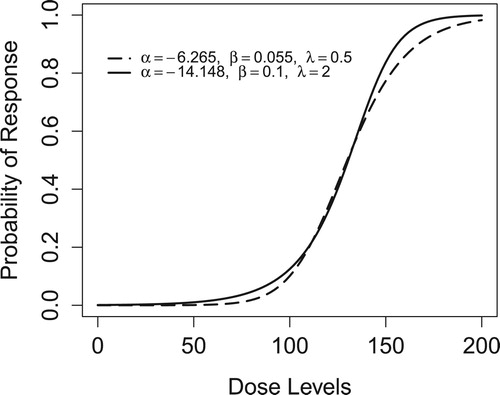
The up-and-down design requires a single target ed level. In the simulation, we always take the middle level as its target. The ed01 and ed99 values under $\lambda =0.5$ are (74, 211); the ed01 and ed99 values under $\lambda =2$ are (49, 180). These values are used to determine the first-stage design Ω. The results are reported in Table 2.

Table 2. RMSEs when fitting data from three-parameter logistic models under a number of designs.

Size	n = 30			n = 60			n = 120
Design	ED	Up-down	D-opt	ED	Up-down	D-opt	ED	Up-down	D-opt
	$\alpha =-6.265$, $\text{β}=0.055$, $\lambda =0.5$
Total	13.32	16.20	16.82	9.87	10.33	11.96	6.93	7.42	8.44
ED10	8.62	9.39	11.33	6.66	6.79	8.16	4.71	4.97	5.82
ED25	6.78	8.09	9.03	4.78	5.05	6.34	3.23	3.61	4.45
ED40	7.55	10.43	8.54	5.50	5.92	6.02	3.93	4.15	4.19
Total	14.02	15.68	16.97	10.49	10.85	11.95	7.47	7.69	8.46
ED25	8.20	8.00	9.03	6.15	5.83	6.33	4.46	4.38	4.45
ED50	6.72	7.68	8.72	4.83	5.06	6.16	3.48	3.51	4.29
ED75	9.17	11.09	11.42	7.00	7.62	8.05	4.88	5.25	5.77
Total	17.36	21.59	22.27	12.63	13.49	16.01	8.89	9.26	11.61
ED60	9.00	9.08	8.94	6.29	6.01	6.45	4.39	4.24	4.60
ED75	8.69	10.64	11.23	5.92	6.45	8.09	4.07	4.34	5.82
ED90	12.04	16.44	17.03	9.22	10.21	12.21	6.57	7.00	8.93
	$\alpha =-14.15$, $\text{β}=0.10$, $\lambda =2.0$
Total	16.76	18.61	21.35	12.26	12.98	15.84	8.92	9.09	11.05
ED10	12.01	12.16	15.58	9.03	9.00	11.63	6.61	6.66	8.22
ED25	8.34	9.44	11.23	5.79	6.38	8.24	4.12	4.45	5.66
ED40	8.21	10.46	9.32	5.93	6.85	6.91	4.35	4.30	4.75
Total	13.05	14.65	16.23	9.36	10.01	11.78	6.76	6.92	8.06
ED25	8.76	8.67	11.23	6.37	6.52	8.24	4.69	4.65	5.66
ED50	6.37	6.32	8.48	4.42	4.42	6.28	3.12	3.25	4.28
ED75	7.28	9.97	8.10	5.25	6.18	5.61	3.74	3.96	3.82
Total	12.32	15.42	16.30	8.67	9.98	11.54	6.23	6.66	8.30
ED60	6.84	7.22	7.93	4.81	4.99	5.77	3.46	3.52	3.89
ED75	6.24	7.63	8.10	4.14	4.96	5.61	2.83	3.27	3.82
ED90	8.12	11.28	11.72	5.90	7.08	8.28	4.35	4.61	6.26

We observe that the RMSEs under each design decrease as n increases. Their sizes are not dramatically different, but those of the D-optimal design are higher. The sequential ED-design has the best overall performance. The up-and-down design gives the lowest RMSEs for a single ed level. This is expected because D-optimality aims for precise estimation of θ, not the ed levels, and the up-and-down design was not intended for the estimation of ed levels under a parametric model. Nevertheless, it is nice to find that the sequential ED-design works well.

4.2. Applying a three-parameter logistic model when two parameters suffice

When the two-parameter logistic model is appropriate but a three-parameter model is assumed, the results are likely suboptimal. In this section, we examine the degree of efficiency loss. We generate dose–response data from the two-parameter logistic regression model and analyse the data under both two-parameter and three-parameter models. We consider only the D-optimal design and the sequential ED-design. The up-and-down design is not included because it does not depend on the model assumption, although the data analysis could be performed under some model assumption.

In this simulation, we generate data from the two-parameter logistic model: $\mathrm{l}\mathrm{o}\mathrm{g}\mathrm{i}\mathrm{t}\left(\pi \right(x\left)\right)=-6.265+0.055x.$ The results are presented in Table 3. The first two columns are obtained under the correct two-parameter model assumption. The D-optimal design in this case is a uniform distribution on ed17.6 and ed82.4, which is well known but not used in applications. The remaining columns are obtained under the three-parameter model, which is also correct but more complex than necessary.

Table 3. RMSEs when fitting three-parameter model to data from two-parameter model.

	Simple logistic model						Three-parameter logistic model
Design	ED-design			D-optimal			ED-design			D-optimal
Size	30	60	120	30	60	120	30	60	120	30	60	120
Total	17.93	13.25	9.35	23.58	15.79	10.87	18.36	13.63	9.88	23.56	17.50	12.41
ED10	12.68	9.48	6.73	17.53	11.96	8.02	12.30	9.60	7.03	17.29	13.04	9.32
ED25	8.93	6.52	4.55	12.15	8.02	5.63	9.55	6.57	4.68	12.03	8.76	6.18
ED40	9.01	6.56	4.63	10.07	6.46	4.69	9.74	7.10	5.13	10.56	7.72	5.37
Total	17.14	12.54	8.74	20.18	12.63	8.87	17.52	12.33	8.86	19.99	14.52	10.22
ED25	10.55	7.80	5.46	12.48	7.70	5.49	10.64	7.80	5.66	12.03	8.76	6.18
ED50	8.12	5.89	4.09	9.89	6.15	4.41	8.45	5.48	4.04	10.33	7.56	5.23
ED75	10.79	7.85	5.46	12.40	7.90	5.39	11.06	7.81	5.48	12.17	8.77	6.23
Total	18.91	13.42	9.40	26.03	15.76	10.58	19.00	13.48	9.92	23.77	17.25	12.49
ED60	9.49	6.64	4.86	9.09	6.45	4.62	9.77	6.97	5.08	10.57	7.70	5.33
ED75	9.39	6.51	4.57	12.87	8.01	5.47	9.43	6.36	4.51	12.17	8.77	6.23
ED90	13.40	9.67	6.63	20.72	11.94	7.79	13.30	9.64	7.22	17.47	12.70	9.42

These results show that the ED-design has advantages over the D-optimal design: the simulated RMSEs under the former are always lower than those under the latter. The efficiency gain can be as much as 40%.

In addition, the use of the more complex three-parameter model does not significantly reduce the efficiency. When we target ed10, ed25, and ed40, the total RMSE increases from 17.93 to 18.36 when the sample size n = 30. This loss is below 2.5%. The worst case is when n = 120: the efficiency loss is 5.6%.

In comparison, the efficiency of the D-optimal design can be strongly affected. When we target ed60, ed75, and ed90 and n = 120, the efficiency loss is as high as 18%. When n = 30, the use of the more complex model makes the D-optimal design more efficient. This may be because that the initial design takes a large proportion of the number of trials.

Overall, if the ED-design is used, the use of a three-parameter model does not greatly affect the efficiency in the estimation of the ed levels.

4.3. Effects under model mis-specification

In this section, we investigate the effect of two kinds of model mis-specification: (a) the dose–response relationship satisfies the three-parameter logistic regression model with $\lambda \ne 1$, and (b) the relationship is not a three-parameter logistic model.

In both situations, we compute the RMSEs of the ed estimates in two settings: the design and analysis are done under (i) the three-parameter model assumption, and (ii) the usual two-parameter model assumption. We examine the accuracy of the design and analysis in both cases.

For (a), we generate data from two three-parameter models: (6) $\mathrm{l}\mathrm{o}\mathrm{g}\mathrm{i}\mathrm{t}\left({\pi }^{\lambda }\right(x\left)\right)=-6.265+0.055x$(6) with $\lambda =0.5$, and (7) $\mathrm{l}\mathrm{o}\mathrm{g}\mathrm{i}\mathrm{t}\left({\pi }^{\lambda }\right(x\left)\right)=-14.148+0.1x$(7) with $\lambda =2$. Under model (6(6) $\mathrm{l}\mathrm{o}\mathrm{g}\mathrm{i}\mathrm{t}\left({\pi }^{\lambda }\right(x\left)\right)=-6.265+0.055x$(6) ), ed25 = 114, ed50 = 130, and ed75 = 148; and under model (7(7) $\mathrm{l}\mathrm{o}\mathrm{g}\mathrm{i}\mathrm{t}\left({\pi }^{\lambda }\right(x\left)\right)=-14.148+0.1x$(7) ), ed25 = 114, ed50 = 130, and ed75 = 144. The results are presented in Table 4. The first two columns are obtained under the two-parameter assumption. The D-optimal design in this case is a uniform distribution on ed17.6 and ed82.4. The remaining columns are obtained under the correct three-parameter assumption.

Table 4. RMSEs when fitting three-parameter model to data from three-parameter model.

	Simple logistic model						Three-parameter logistic model
Design	ED-design			D-optimal			ED-design			D-optimal
Size	30	60	120	30	60	120	30	60	120	30	60	120
	$\alpha =-6.265$, $\text{β}=0.055$, $\lambda =0.5$
Total	13.87	9.96	7.16	16.62	13.38	11.04	13.32	9.87	6.93	16.82	11.96	8.44
ED10	10.14	7.08	4.99	11.75	9.50	7.77	8.62	6.66	4.71	11.33	8.16	5.82
ED25	6.53	4.74	3.43	8.63	7.15	6.09	6.78	4.78	3.23	9.03	6.34	4.45
ED40	6.86	5.17	3.82	7.97	6.14	4.94	7.55	5.50	3.93	8.54	6.02	4.19
Total	15.57	11.14	7.65	15.72	11.46	8.69	14.02	10.49	7.47	16.97	11.95	8.46
ED25	9.45	6.63	4.30	8.63	7.15	6.09	8.20	6.15	4.46	9.03	6.34	4.45
ED50	6.64	5.06	3.57	8.12	5.82	4.30	6.72	4.83	3.48	8.72	6.16	4.29
ED75	10.44	7.39	5.22	10.34	6.81	4.47	9.17	7.00	4.88	11.42	8.05	5.77
Total	18.98	12.89	8.98	19.80	13.86	10.23	17.36	12.63	8.89	22.40	15.83	11.48
ED60	8.16	5.78	4.23	8.65	5.82	3.90	9.00	6.29	4.39	9.33	6.58	4.63
ED75	8.74	5.90	4.21	10.34	6.81	4.47	8.69	5.92	4.07	11.42	8.05	5.77
ED90	14.73	9.89	6.71	14.50	10.57	8.34	12.04	9.22	6.57	16.86	11.94	8.78
	$\alpha =-14.15$, $\text{β}=0.10$, $\lambda =2.0$
Total	17.43	12.39	8.99	24.82	15.78	12.04	16.76	12.26	8.92	21.35	15.84	11.05
ED10	14.00	9.78	6.98	19.42	12.80	10.33	12.01	9.03	6.61	15.58	11.63	8.22
ED25	7.50	5.40	3.95	12.51	7.47	5.11	8.34	5.79	4.12	11.23	8.24	5.66
ED40	7.19	5.35	4.06	9.07	5.42	3.50	8.21	5.93	4.35	9.32	6.91	4.75
Total	13.80	9.57	6.95	16.25	10.09	6.93	13.05	9.36	6.76	16.23	11.78	8.06
ED25	9.43	6.64	4.76	12.51	7.47	5.11	8.76	6.37	4.69	11.23	8.24	5.66
ED50	5.95	4.25	3.47	7.52	4.69	3.13	6.37	4.42	3.12	8.48	6.28	4.28
ED75	8.14	5.43	3.70	7.13	4.90	3.49	7.28	5.25	3.74	8.10	5.61	3.82
Total	13.06	8.75	6.35	15.63	10.30	7.10	12.32	8.67	6.23	16.30	11.54	8.30
ED60	6.27	4.57	3.49	6.59	4.37	3.06	6.84	4.81	3.46	7.93	5.77	3.89
ED75	6.22	4.08	2.96	7.13	4.90	3.49	6.24	4.14	2.83	8.10	5.61	3.82
ED90	9.63	6.25	4.40	12.25	7.93	5.37	8.12	5.90	4.35	11.72	8.28	6.26

We observe that the ED-design is noticeably superior to the D-optimal design in both situations: the simulated RMSEs under the former are always lower than those under the latter. The efficiency gain can be as much as 30%.

In addition, the use of the three-parameter model when the data are generated under that model significantly increases efficiency. When $\lambda =0.5$ and we target ed25, ed50, and ed75, the total RMSE decreases from 15.57 to 14.02 when n = 30, a gain of 11%. Overall, the use of the three-parameter model makes the ED-design more efficient.

For (b), we generate data from the three-parameter probit model: (8) $\pi \left(x\right)={\mathrm{\Phi }}^{1/\lambda }(-6.265+0.055x)$(8) with $\lambda =0.5$, and (9) $\pi \left(x\right)={\mathrm{\Phi }}^{1/\lambda }(-14.148+0.1x)$(9) with $\lambda =2$. Under this model, ed25 = 114, ed50 = 124, and ed75 = 134 when $\lambda =0.5$; and ed25 = 86, ed50 = 102, and ed75 = 117 when $\lambda =2$. The results are presented in Table 5. The first two columns are obtained under the two-parameter assumption. The D-optimal design in this case is a uniform distribution on ed12.8 and ed87.2. The remaining columns are obtained under the three-parameter assumption. Both model assumptions are incorrect, but is it better to use the three-parameter logistic model with the ED-design?

Table 5. RMSEs when fitting three-parameter model to data from probit model.

	Simple logistic model						Three-parameter logistic model
Design	ED-design			D-optimal			ED-design			D-optimal
Size	30	60	120	30	60	120	30	60	120	30	60	120
	$\alpha =-6.265$, $\text{β}=0.055$, $\lambda =0.5$
Total	9.27	6.29	4.31	9.02	6.81	7.48	8.58	5.75	4.25	12.36	7.65	4.95
ED10	6.68	4.49	3.01	5.44	3.98	4.69	5.76	3.94	2.94	7.24	4.40	3.14
ED25	4.36	3.08	2.11	4.85	3.86	4.37	4.42	2.85	2.06	7.11	4.41	2.77
ED40	4.72	3.16	2.24	5.31	3.95	3.85	4.57	3.08	2.27	7.06	4.43	2.64
Total	9.73	6.22	4.38	10.29	7.28	6.40	8.57	6.00	4.25	12.09	7.56	4.83
ED25	6.22	3.91	2.72	4.85	3.86	4.37	5.17	3.70	2.68	7.11	4.41	2.77
ED50	4.18	2.71	2.00	5.72	4.06	3.52	4.27	2.85	2.00	6.99	4.41	2.65
ED75	6.21	4.01	2.80	7.05	4.65	3.07	5.34	3.77	2.61	6.84	4.28	2.94
Total	10.17	6.71	4.45	12.75	8.38	5.64	9.14	6.52	4.58	12.55	7.71	5.26
ED60	5.05	3.29	2.21	6.19	4.23	3.25	4.77	3.45	2.47	6.89	4.36	2.72
ED75	4.78	3.17	2.14	7.05	4.65	3.07	4.49	3.07	2.12	6.84	4.28	2.94
ED90	7.41	4.90	3.21	8.63	5.55	3.44	6.37	4.60	3.22	7.94	4.70	3.42
	$\alpha =-14.15$, $\text{β}=0.10$, $\lambda =2.0$
Total	8.52	5.65	3.70	8.75	5.95	4.31	8.39	5.43	3.13	12.89	7.62	4.33
ED10	6.33	4.13	2.67	6.24	4.19	3.05	5.81	3.80	2.13	9.13	5.16	2.80
ED25	3.97	2.69	1.79	4.63	3.10	2.16	4.24	2.67	1.57	6.67	4.02	2.39
ED40	4.09	2.75	1.83	4.04	2.87	2.14	4.32	2.82	1.68	6.19	3.91	2.28
Total	8.25	5.39	3.52	7.51	5.80	4.77	7.33	5.21	3.66	10.47	6.59	4.21
ED25	5.42	3.50	2.28	4.63	3.10	2.16	4.59	3.21	2.31	6.67	4.02	2.39
ED50	3.40	2.36	1.57	3.93	3.00	2.41	3.67	2.57	1.78	5.98	3.82	2.24
ED75	5.20	3.36	2.17	4.43	3.89	3.50	4.37	3.19	2.21	5.42	3.57	2.66
Total	8.29	5.30	3.55	8.29	7.05	6.24	7.12	5.06	3.65	9.63	6.39	4.99
ED60	3.97	2.66	1.79	3.99	3.27	2.80	3.97	2.77	2.05	5.76	3.70	2.29
ED75	3.87	2.51	1.71	4.43	3.89	3.50	3.76	2.51	1.71	5.42	3.57	2.66
ED90	6.17	3.84	2.55	5.76	4.88	4.33	4.56	3.41	2.48	5.48	3.79	3.54

Clearly, the ED-design is noticeably superior to the D-optimal design in both situations: the simulated RMSEs under the former are always lower than those under the latter. When $\lambda =2$ and we target ed10, ed25, and ed40, the total RMSE decreases from 12.89 to 8.39 when n = 30, a gain of 54%.

In addition, the use of the more complex model when the data are generated under the three-parameter probit model noticeably increases the efficiency. When we target ed60, ed75, and ed90 with $\lambda =2$ the total RMSE decreases from 8.29 to 7.12 when n = 30, a gain of 16%. Overall, combining the more complex model with the ED-design leads to efficiency gains when the model is mis-specified.

4.4. Example

Brown (1982) assumed a three-parameter logistic response model for the relationship between the wheezing symptom and the age of British coal miners. The number of subjects examined and the number with the symptom can be found in their paper.

We first fit the observed data using model (2(2) $\mathrm{l}\mathrm{o}\mathrm{g}\mathrm{i}\mathrm{t}\left\{{\pi }^{\lambda }\right(x\left)\right\}=\log \left\{\frac{{\pi }^{\lambda }\left(x\right)}{1-{\pi }^{\lambda }\left(x\right)}\right\}=\alpha +\text{β}x.$(2) ). The MLEs of the model parameters are $\hat{\alpha }=-1.798$, $\widehat{\text{β}}=0.044$, and $\hat{\lambda }=0.400$. We then fit the observed data using a simple logistic model. The MLEs of the model parameters are $\hat{\alpha }=-4.225$ and $\widehat{\text{β}}=0.065$. For comparison, Figure 2 shows the observed data and the two fitted curves.

Figure 2. Observed data and fitted curves for British coal miners.

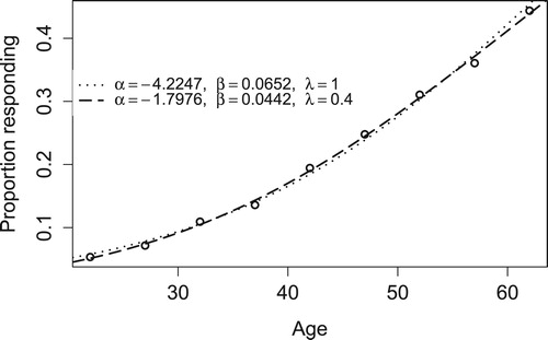
Based on fitted two-parameter and three-parameter models, the age at which 25% coal miners will develop the symptoms is 47.7 and 48.1, respectively. Both match the real data closely. The three-parameter model predicts the ages at which 50% and 75% of miners develop the symptoms are 66.8 and 88.7, respectively. In comparison, these figures are 65.0 and 81.9 based on the two-parameter model. While two models give very different numbers, predicting the proportion based on either model is not reliable at age 80 due to extreme extrapolation. At each observed ED level, we compute the corresponding age based on fitted models and the difference to the observed age. The resulting sum of squares (weighted) is 6906 for the three-parameter model and 15,420 for the two-parameter model. The use of the three-parameter model provides a much-improved fit.

5. Concluding remarks

We have explored the use of a three-parameter logistic regression model for dose–response experiments. The sequential ED-design can easily be applied to this model, and the resulting data analysis is effective.

Simulation results show that the three-parameter logistic regression model is an effective extension of the commonly used two-parameter model that does not lead to more complex data analysis issues. The combination of the ED-design and the data analysis strategy works well. When the logistic model is correct, the more complex model has hardly any efficiency loss. When the three-parameter model holds but the logistic model is violated, the new approach gains substantial ground. It will be a useful addition to the toolbox for dose–response experiments.

Acknowledgments

The authors gratefully acknowledge the fundings from the National Natural Science foundation of China, 11871419 and the Natural Science and Engineering Research Council of Canada.

Disclosure statement

No potential conflict of interest was reported by the author(s).

Additional information

Funding

The authors gratefully acknowledge the fundings from the National Natural Science foundation of China [Grant Number 11871419] and the Natural Science and Engineering Research Council of Canada.

Notes on contributors

Xiaoli Yu

Dr. Xiaoli Yu is currently self-employed.

Shaoting Li

Dr. Shaoting Li is an associate professor at the School of Statistics, Dongbei University of Finance and Economics.

Jiahua Chen

Jiahua Chen is Canada Research Chair, tier I at the Department of Statistics, University of British Columbia.

References

- Brown, C. C. (1982). On a goodness of fit test for the logistic model based on score statistics. Communications in Statistics - Theory and Methods, 11(10), 1087–1105. https://doi.org/10.1080/03610928208828295
- El-Saidi, M. A. (1993). A power transformation for generalized logistic response function with application to quantal bioassay. Biometrical Journal, 35(6), 715–726. https://doi.org/10.1002/(ISSN)1521-4036 doi: https://doi.org/10.1002/bimj.4710350609
- Fedorov, V. V. (1972). Theory of optimal experiments. Elsevier.
- Ford, I., Titterington, D. M., & Wu, C. F. J. (1985). Inference and sequential design. Biometrika, 72(3), 545–551. https://doi.org/10.1093/biomet/72.3.545
- Li, G., & Majumdar, D. (2008). D-optimal designs for logistic models with three and four parameters. Journal of Statistical Planning and Inference, 138(7), 1950–1959. https://doi.org/10.1016/j.jspi.2007.07.010
- Li, P., & Wiens, D. P. (2011). Robustness of design in dose-response studies. Journal of the Royal Statistical Society: Series B (Statistical Methodology), 73(2), 215–238. https://doi.org/10.1111/rssb.2011.73.issue-2 doi: https://doi.org/10.1111/j.1467-9868.2010.00763.x
- O'Brien, T. E., Chooprateep, S., & Homkham, N. (2009). Efficient geometric and uniform design strategies for sigmoidal regression models. South African Statistical Journal, 43(1), 49–83. https://journals.co.za/content/sasj/43/1/EJC119263.
- Sitter, R. R., & Fainaru, I. (1997). Optimal designs for the logit and probit models for binary data. Canadian Journal of Statistics, 25(2), 175–190. https://doi.org/10.2307/3315730
- Sitter, R. R., & Forbes, B. (1997). Optimal two-stage designs for binary response experiments. Statistica Sinica, 7(4), 941–955. https://doi.org/10.2307/3315730.
- Sitter, R. R., & Wu, C. (1993). Optimal designs for binary response experiments: Fieller, D, and A criteria. Scandinavian Journal of Statistics, 20(4), 329–341.
- Wang, L., Liu, Y., Wu, W., & Pu, X. (2013). Sequential LND sensitivity test for binary response data. Journal of Applied Statistics, 40(11), 2372–2384. https://doi.org/10.1080/02664763.2013.817546
- Wu, C. (1978). Some algorithmic aspects of the theory of optimal designs. The Annals of Statistics, 6(6), 1286–1301. https://doi.org/10.1214/aos/1176344374
- Wu, C. F. J. (1985). Efficient sequential designs with binary data. Journal of the American Statistical Association, 80(392), 974–984. https://doi.org/10.1080/01621459.1985.10478213
- Wu, C. F. J., & Tian, Y. (2014). Three-phase optimal design of sensitivity experiments. Journal of Statistical Planning and Inference, 149, 1–15. https://doi.org/10.1016/j.jspi.2013.10.007
- Wynn, H. P. (1972). Results in the theory and construction of D-optimum experimental designs. Journal of the Royal Statistical Society, Series B, 34(2), 133–147.
- Yu, X., Chen, J., & Brant, R. (2016). Sequential design for binary dose-response experiments. Journal of Statistical Planning and Inference, 177, 64–73. https://doi.org/10.1016/j.jspi.2016.04.005