Target toxicity design for phase I dose-finding

Abstract

We propose a new two-/three-stage dose-finding design called Target Toxicity (TT) for phase I clinical trials, where we link the decision rules in the dose-finding process with the conclusions from a hypothesis test. The power to detect excessive toxicity is also given. This solves the problem of why the minimal number of patients is needed for the selected dose level. Our method provides a statistical explanation of traditional ‘3+3’ design using frequentist framework. The proposed method is very flexible and it incorporates other interval-based decision rules through different parameter settings. We provide the decision tables to guide investigators when to decrease, increase or repeat a dose for next cohort of subjects. Simulation experiments were conducted to compare the performance of the proposed method with other dose-finding designs. A free open source R package tsdf is available on CRAN. It is dedicated to deriving two-/three-stage design decision tables and perform dose-finding simulations.

Keywords:

• Group-sequential-like designs
• dose-finding
• phase I
• MTD
• recommended phase II doses
• power

1. Introduction

The primary goal of a phase I oncology trial is to determine the recommended phase II doses (RP2Ds). These RP2Ds are at or below the maximum tolerated dose (MTD). The MTD is defined as the highest dose of a drug or treatment that does not cause unacceptable side effects/toxicity. The common procedure to find RP2D/MTD is as follows: treat a cohort of patients with a predetermined dose and then based on the observed binary outcome dose-limiting toxicity (DLT) to adjust dose level accordingly. The trial usually starts with the lowest dose level and enrol more patients sequentially until an RP2D is found, or MTD is reached or maximum sample size is reached. Due to limited information regarding the toxicity of new treatment and small sample size in phase I study, the estimation of RP2D or MTD suffers from low precision. Since the usual way to find RP2Ds is to find MTD first (if possible), then look for doses at or below MTD for RP2Ds. We will focus on how to find MTD in the rest of the paper.

Both rule-based and model-based designs have been proposed for phase I dose-finding. The most commonly used rule-based method is the traditional ‘3+3’ design. The advantage of the ‘3+3’ design is its transparent and easy to implement nature. However, various simulations have demonstrated that ‘3+3’ design identifies the MTD in as few as 30% of trials (Reiner et al., 1999). Also, the mechanisms of these rule-based designs are non-transparent which requires intensive simulations under different settings to understand the operating characteristics. Other variations based on ‘3+3’ design, such as accelerated titration designs, ‘2+4’, ‘3+3+3’ (Storer, 2001) are proposed to improve the precision. Model-based designs establish a dose-toxicity curve prior to patient enrolment and modify the estimates of the probability of toxicities for each dose level as study proceeds. The most popular model-based method is the continual reassessment method (CRM) (O'Quigley et al., 1990). The main idea of CRM is to assign as many patients as we can on doses close to the MTD. Several concerns have been raised about the safety of CRM since it may overestimate dose for MTD. In addition, model-based designs require to provide prior estimates of probability toxicities for predetermined dose and must run intensive simulations to achieve desirable operating characteristics. Therefore, the application of CRM tends to be especially challenging in term of parameters tuning and computation. Some modifications to CRM and tools are developed to overcome these issues, such as modified CRM and R package dfCRM (Cheung, 2013; Cheung & Chappell, 2000; Goodman et al., 1995). Another class of model-based designs is called interval-based designs. The interval-based designs are based on parametric model and make inference using posterior probabilities of three dosing intervals. The advantage of interval-based designs, such as mTPI, mTPI-2 (Guo et al., 2017; Ji et al., 2010), is that they provide a decision table with all dose-finding decision (see example in Table 1), which is easier to examine and the decision table can be adjusted before the trial starts. However, the statistical theory behind interval-based designs is not trivial and such designs also assume the toxicity rate for predetermined dose level follows a prior distribution which could be debated in practice.

Table 1. A decision table for a ‘3+3+3’ design (target toxicity is 0.3).

DLTs	# of subjects
	3	6	9
0	E	E	E
1	S	E	E
2	D	S	E
3	DU	D	S
4		DU	D
5		DU	DU
6		DU	DU
7			DU
8			DU
9			DU

Notes: Row represents number of DLTs. Column represents number of subjects. ‘E’: escalate dose level; ‘S’: stay at current dose level; ‘D’: de-escalate dose level; ‘DU’: de-escalate and never come back to this dose level again.

In this article, we propose new two-/three-stage designs to solve the problems in existing methods. We provide two-/three-stage decision tables similar to other interval-based designs such as TPI, mTPI, BOIN, CCD (Ivanova et al., 2007; Ji et al., 2007; Liu & Yuan, 2015; Yuan et al., 2016). The difference between the proposed method and commonly used rule-based or model-based designs is that we find the decision rules using hypothesis testing approach. The dose-finding procedure aims to find the highest dose level that the toxicity probability is less than or equal to a target toxicity which can be converted to a hypothesis test: is the probability of toxicity at current dose level different from the target toxicity? If there is sufficient evidence to show that the probability of toxicity is lower than the target, then we need to escalate dose level; on the contrary, we should de-escalate the dose level. Therefore, the corresponding rejection regions link to the decision rules naturally. For example, if the rejection regions are $[0,r]$ and $(s,n]$, dose-escalation would be beneficial if the number of DLTs among n patients is less than or equal to r, or de-escalation is recommended when the number of DLTs is more than s. Otherwise, more patients should be enrolled and tested at the current dose level. The boundaries in the rejection regions are controlled by the cumulative type I error and can be chosen to be dependent on the sample size. We will show in the following sections that the proposed method is not only as transparent and simple as ‘3+3’ design but also provides a statistical framework as model-based methods. Moreover, it is extremely flexible and retains the interpretability. Simply by modifying the type I error, we can incorporate an aggressive, a conservative or the same decision rules as other model-based designs.

The remainder of the paper is organised as follows. Section 2 is devoted to the mechanism of two- and three-stage designs. Section 3 introduces an R package tsdf that implements our method and conducts dose-finding simulations using customised decision table. Simulation results are presented in Section 4. Some discussions are given in the last section.

2. Phase I dose-finding

The ‘up-and-down’ design for dose-finding procedure is as follows: based on observed values of number of patients treated and experienced dose-limiting toxicity (DLT) at current dose level, there are four different decisions for the next step: stay at current dose level (S), escalate to a higher dose level (E), de-escalate to a lower dose level (D) or de-escalate and never go back to current dose again (DU). Then the next cohort of patients is treated at a dose level based on the decision just made. This procedure is repeated until the MTD or maximum sample size is reached. The set of decision rules forms a table, we call it a decision table (See example in Table 1). Our goal is to find the optimal decision table to guide investigators when choosing a proper decision among ‘D’, ‘S’, ‘E’ and ‘DU’.

The dose-finding problem can be considered as a hypothesis test: is the probability of toxicity at current dose level different from the target toxicity? Denote the target toxicity as $p_t$, the hypotheses are set as (1) $H_0:p=p_t\mathrm{v}.\mathrm{s}.H_1:p\ne p_t.$(1) Note that the alternative can be decomposed as two parts: (2) $H_1^{-}:p<p_t\mathrm{and}{H}_1^{+}:p>p_t.$(2) There are three possible conclusions for the above hypothesis test: do not reject null hypothesis, reject null and conclude $H_1^{+}$, and reject null and conclude $H_1^{-}$. In dose-finding context, it means we may conclude that the probability of toxicity is equal, higher or lower than the target toxicity. By carrying out such hypothesis test based on observed values, we choose to either stay at current dose level, escalate dose level or de-escalate dose level, then enrol more patients to the trial. This hypothesis test also can be generalised to the case that the target toxicity is not a single value but a pre-specified interval. The hypothesis becomes (3) $H_0:p\in [p_l,p_u]\mathrm{v}.\mathrm{s}{H}_1:p\notin [p_l,p_u],$(3) where $p_u>p_l$. Also, the alternative is decomposed as: (4) $H_1^{-}:p<p_l\mathrm{and}{H}_1^{+}:p>p_u.$(4) The design becomes more flexible when the target toxicity is an interval. For example, interval-based dose-finding designs usually use interval $(p_t-{ϵ}_1,p_t+{ϵ}_2)$, where ${ϵ}_1$ and ${ϵ}_2$ are two small fractions that reflect investigator's desire about how accurate they want the MTD to be around the target $p_t$ (Ji & Yang, 2017). Also, test in (3(3) $H_0:p\in [p_l,p_u]\mathrm{v}.\mathrm{s}{H}_1:p\notin [p_l,p_u],$(3) ) is equivalent to test in (1(1) $H_0:p=p_t\mathrm{v}.\mathrm{s}.H_1:p\ne p_t.$(1) ) by letting $p_l=p_u=p_t.$

Denote $x_i$ as the cumulative number of subjects experienced DLT among $n_1+n_2+\cdots +n_i$ at Stage i of a particular dose. The corresponding left-side critical values are $r_i$'s and right-side critical values are $s_i$'s. In general, the following decisions are made:

• If $x_i\le r_i$, conclude $H_1^{-}$ and escalate dose level;

• If $x_i>s_i$, conclude $H_1^{+}$ and de-escalate dose level;

• If $r_i<x_i\le s_i$, stay at current dose level and treat an additional $n_{i+1}$ subjects if maximum sample size is not reached.

Note that at stage i, $n_i$ subjects are treated and this procedure can be repeated until the maximum sample size is reached. Although the above procedure can be extended to multiple stages, for practical purposes, we consider only two-stage and three-stage designs in this article. Note that $r_i$ and $s_i$ are determined by significance level or left-side and right-side type I error. Denote the overall left-side type I error as ${\alpha }_1$, right-side type I error as ${\alpha }_2$, and the type 2 error as β. We use the α-spending function to distribute the overall type I error over two/three stages. The cumulative left-side type I errors at stage i are ${\alpha }_{1i}$'s, where ${\alpha }_{11}\le {\alpha }_{12}\dots$ and the cumulative right-side type I errors are ${\alpha }_{2i}$'s, where ${\alpha }_{21}\le {\alpha }_{22}\dots$. We have the following error constraints:

• if $p=p_l$, the probability should not exceed ${\alpha }_{1i}$ (left-side type I error) to conclude $H_1^{-}$;

• if $p=p_u$, the probability should not exceed ${\alpha }_{2i}$ (right-side type I error) to conclude $H_1^{+}$;

• if the excessive toxicity probability is $p_e$ ($>p_u$), then the probability of not concluding $H_1^{+}$ should not exceed β.

Before we give details of two-stage designs and three-stage designs in the following subsections, let's look at our hypotheses to get an idea of how error constraints affect dose-escalation strategy. The type I error is the probability of rejecting the true null hypothesis. For left-side, high type I error means that it's more likely to conclude $H_1^{-}$, i.e., it's easier to escalate dose level. Thus, high left-side type I error designs lead to more aggressive designs than low left-side type I error ones. Right-side is the opposite: low right-side type II error is more aggressive since rejecting null hypothesis lead to de-escalate the dose level. Investigators can choose a suitable design by giving specific left-side, right-side type I errors and type II error, respectively. Investigators can also choose different designs at different dose-finding stages. For example, they can choose more aggressive designs at early stages similar to accelerated titration designs. In general, the decision table generated by our method includes the familiar ‘3+3’ design, interval-based method such as mTPI, mTPI-2, but more importantly a wide variety of more flexible designs.

Unlike traditional ‘3+3’ design, the proposed two/three-stage designs do not restrict the cohort size to be fixed, hence more flexible when cohort size, typically ranging from say 1-6, varies. For instance, two-stage designs and three-stage designs proceed in a ‘A+B’ and ‘A+B+C’ fashion, respectively. As a result, our method can be used in a variety of situations, such as ‘2+4’, or ‘2+4+8’. We describe two-stage designs in Section 2.1, three-stage designs in Section 2.2 and explain how to produce decision table in Section 2.3.

2.1. Two-stage designs

The dose-finding procedure using a two-stage design is an iteration process. The two-stage design (‘A+B’) setup of a particular dose level is: $n_1$ patients are treated in the first stage. If the trial continues the dose level to the second stage, additional $n_2$ patients are treated. Recall that $x_i$ is the total cumulative number of patients experienced DLT until stage i. The procedure is as follows ($r_i\le s_i,r_1\le r_2,s_1\le s_2,r_i\le \sum _1^i{n}_k,s_i\le \sum _1^i{n}_k$):

1. Stage 1: treat $n_1$ patients

   	•	If $x_1\le r_1$, escalate to next higher dose level (conclude $H_1^{-}$);
   	•	If $x_1>s_1$, de-escalate to next lower dose level (conclude $H_1^{+}$);
   	•	If $r_1<x_1\le s_1$, stay at current dose level and go to stage 2.

2. Stage 2: treat additional $n_2$ patients

   	•	If $x_2\le r_2$, escalate to next higher dose level;
   	•	If $x_2>s_2$, de-escalate to next lower dose level;
   	•	If $r_2<x_2\le s_2$, stay at current dose level. This dose level is MTD.

Denote the binomial cumulative density function as $B(\cdot ;n,p)$ and probability function as $b(\cdot ,n,p)$, where n is the number of Bernoulli trials, p is the probability of success. Let's calculate the conditional probabilities. If the true toxicity rate is p, then the probability of concluding $H_1^{-}$ at the first stage is (5) $L_1(p)=B(r_1,n_1,p)$(5) and at the second stage is (6) $L_2(p)=\sum _{t_1=r_1+1}^{s_1}b(t_1,n_1,p)B(r_2-t_1,n_2,p).$(6) Similarly, the probabilities of concluding $H_1^{+}$ at two stages are (7) $\begin{array}{rl}{R}_1(p)& =1-B(s_1,n_1,p)\mathrm{and}\\ R_2(p)& =\sum _{t_1=r_1+1}^{s_1}b(t_1,n_1,p)[1-B(s_2-t_1,n_2,p)].\end{array}$(7) The design is a group-sequential-like design. Hence, lower and upper type I error ${\alpha }_1$ can be spent following an error spending method. For any chosen error spending function, error rate ${\alpha }_{i1}\le {\alpha }_{i2}={\alpha }_i$ allowed at each stage can be calculated. Therefore, $r_i,s_i$ have to satisfy the following type I error constraints (8) $L_1(p_l)\le {\alpha }_{11},L_1(p_l)+L_2(p_l)\le {\alpha }_{12}={\alpha }_1$(8) and (9) $R_1(p_u)\le {\alpha }_{21},R_1(p_u)+R_2(p_u)\le {\alpha }_{22}={\alpha }_2.$(9) The type II error constraint is (10) $\sum _{i=1}^2{R}_i(p_e)\ge 1-\beta .$(10) The focus is to pursue designs that have the closest errors to the desired left-side and right-side type I errors (but $\le {\alpha }_{i1}$ at Stage 1 and $\le {\alpha }_{i2}={\alpha }_1$ at Stage 2 from a chosen α-spending function) and the minimal sample size n under the toxicity level the trial is designed to detect. In addition, it is also desirable to minimise β for a given n. With the conditions (8(8) $L_1(p_l)\le {\alpha }_{11},L_1(p_l)+L_2(p_l)\le {\alpha }_{12}={\alpha }_1$(8) ), (9(9) $R_1(p_u)\le {\alpha }_{21},R_1(p_u)+R_2(p_u)\le {\alpha }_{22}={\alpha }_2.$(9) ) outlined, there are usually many designs with combinations of ($r_i,s_i$) that satisfy type I and II error constraints. Therefore, additional selection criteria are needed to choose designs that satisfy practical considerations. For a given n, at each stage of 1 and 2, all possible combinations of $r_i,s_i$ satisfying type I error (Stage 1 and 2) are outputted into a matrix in R. Each combination of $r_i,s_i$ forms a feasible design and all feasible designs are sorted in descending order by the actual left-side, right-side type I errors, and $1-\beta$. The first design is then chosen. This design has the closest type I error to ${\alpha }_{11}$, ${\alpha }_{21}$, ${\alpha }_{12}$ and ${\alpha }_{22}$, and 1 - β.

2.2. Three-stage designs

Three-stage design (‘A+B+C’) is an extension of two-stage design where we treat additional $n_3$ patients if the decision is to stay at current dose level at stage 2 or the trial comes back to this dose level. Thus, the sample size for each dose is at most $n_1+n_2+n_3=n$. The complete three-stage design is as follows:

1. Stage 1: treat $n_1$ patients

   	•	If $x_1\le r_1$, escalate to next higher dose level dose level;
   	•	If $x_1>s_1$, de-escalate to next lower dose level;
   	•	If $r_1<x_1\le s_1$, stay at current dose level and go to Stage 2.

2. Stage 2: treat additional $n_2$ patients

   	•	If $x_2\le r_2$, escalate to next high dose level;
   	•	If $x_2>s_2$, de-escalate to next lower dose level;
   	•	If $r_2<x_2\le s_2$, stay at current dose level and go to Stage 3.

3. Stage 3: treat additional $n_3$ patients

   	•	If $x_3\le r_3$, escalate to next higher dose level;
   	•	If $x_3>s_3$, de-escalate to next lower dose level;
   	•	If $r_3<x_3\le s_3$, stay at current dose level. This dose level is MTD.

Then we only need to calculate the conditional probabilities at the third stage in addition to the first two stages that have been calculated in previous subsection. The probability of concluding $H_1^{-}$ at the third stage is

(11) $\begin{array}{rl}{L}_3(p)& =\sum _{t_1=r_1+1}^{s_1}\sum _{t_2=r_2-t_1+1}^{s_2-t_1}b(t_1,n_1,p)b(t_2,n_2,p)B(r_3-t_1-t_2,n_3,p).\end{array}$(11) and concluding $H_1^{+}$ at the third stage is (12) $\begin{array}{rl}{R}_3(p)& =\sum _{t_1=r_1+1}^{s_1}\sum _{t_2=r_2-t_1+1}^{s_2-t_1}b(t_1,n_1,p)b(t_2,n_2,p)[1-B(s_3-t_1-t_2,n_3,p)].\end{array}$(12)

Combining (11(11) $\begin{array}{rl}{L}_3(p)& =\sum _{t_1=r_1+1}^{s_1}\sum _{t_2=r_2-t_1+1}^{s_2-t_1}b(t_1,n_1,p)b(t_2,n_2,p)B(r_3-t_1-t_2,n_3,p).\end{array}$(11) ) with (5(5) $L_1(p)=B(r_1,n_1,p)$(5) ), (6(6) $L_2(p)=\sum _{t_1=r_1+1}^{s_1}b(t_1,n_1,p)B(r_2-t_1,n_2,p).$(6) ) and (11(11) $\begin{array}{rl}{L}_3(p)& =\sum _{t_1=r_1+1}^{s_1}\sum _{t_2=r_2-t_1+1}^{s_2-t_1}b(t_1,n_1,p)b(t_2,n_2,p)B(r_3-t_1-t_2,n_3,p).\end{array}$(11) ), $r_i,n_i$ have to satisfy the following constraints: (13) $\sum _{k=1}^i{L}_k(p_l)\le {\alpha }_{1i}\mathrm{and}\sum _{k=1}^i{R}_k(p_u)\le {\alpha }_{2i},$(13) for i = 1, 2, 3 and (14) $\sum _{i=1}^3{R}_i(p_e)\ge 1-\beta .$(14) The optimal design is chosen as described in the end of Section 2.1.

2.3. Decision table

Decision table allows investigators to examine the design before the trial starts, which consists of four decision rules: stay at current dose level (S), escalate to a higher dose level (E), de-escalate to a lower dose level (U) or de-escalate and never go back to current dose again (DU) (See example in Table 1). The two-stage and three-stage designs in Sections 2.1 and 2.2 provide decision rule ‘D’, ‘S’ and ‘E’ in the decision table: $x_i\le r_i⟶\text{`E'}$; $x_i>s_i⟶\text{`D'}$; $r_i<x_i\le s_i⟶\text{`S'}$. To prevent exposing patients to dose level of excessive toxicity, we propose to perform another one-sided test to put ‘DU’ (De-escalate/Unacceptable) in the table: (15) $H_0^u:p=p_u\mathrm{v}.\mathrm{s}.H_1^u:p>p_u.$(15) The procedure is as follows:

• If $x_i>u_i$, conclude $H_1^u$, de-escalate dose level and never go back to this dose level,

where $u_i$'s should satisfy the following requirements:?>

• if $p=p_u$, the probability should not exceed ${\alpha }_{ui}$ (cumulative type I error, calculated by $\alpha -$spending method) to conclude $H_1^u$ in (15(15) $H_0^u:p=p_u\mathrm{v}.\mathrm{s}.H_1^u:p>p_u.$(15) ).

The probabilities of concluding $H_1^u$ at three stages are (16) $\begin{array}{rl}{R}_1(p)& =1-B(u_1,n_1,p),\\ R_2(p)& =\sum _{t_1=0}^{u_1}b(t_1,n_1,p)[1-B(u_2-t_1,n_2,p)],\\ R_3(p)& =\sum _{t_1=0}^{u_1}\sum _{t_2=0}^{u_2-t_1}b(t_1,n_1,p)b(t_2,n_2,p_t)\\ & \times [1-B(u_3-t_1-t_2,n_3,p)].\end{array}$(16) For two-stage designs(${\alpha }_{u2}={\alpha }_u$), $u_i$'s satisfy (17) $\sum _{k=1}^i{R}_k(p_u)\le {\alpha }_{ui},\mathrm{for}i=1,2.$(17) For three-stage designs (${\alpha }_{u3}={\alpha }_u$), $u_i$'s satisfy (18) $\sum _{k=1}^i{R}_k(p_u)\le {\alpha }_{ui},\mathrm{for}i=1,2,3.$(18) All the rest is the same.

To summarise (in Table 2):

• Test $H_0:p\in [p_l,p_u]$ v.s. $H_1:p\notin [p_l,p_u]$ produces decision ‘D’, ‘S’, ‘E’. We need to specify left-side type I error ${\alpha }_1$, right-side type I error ${\alpha }_2$ and type II error β. The design satisfies (13(13) $\sum _{k=1}^i{L}_k(p_l)\le {\alpha }_{1i}\mathrm{and}\sum _{k=1}^i{R}_k(p_u)\le {\alpha }_{2i},$(13) ) and (14(14) $\sum _{i=1}^3{R}_i(p_e)\ge 1-\beta .$(14) ).

• Test $H_0:p=p_u$ v.s. $H_1:p>p_u$ produces decision ‘DU’. The design satisfies (17(17) $\sum _{k=1}^i{R}_k(p_u)\le {\alpha }_{ui},\mathrm{for}i=1,2.$(17) ) or (18(18) $\sum _{k=1}^i{R}_k(p_u)\le {\alpha }_{ui},\mathrm{for}i=1,2,3.$(18) ) for two-stage designs and three-stage designs, respectively. The type I error ${\alpha }_u$ for this test should be less than ${\alpha }_2$ in the first test.

Table 2. Rejection regions and decision rules.

Conclusion	Rejection region	Decision rule
Higher than target	$(s,u]$	De-escalate(D)
Much higher than target	$(u,n]$	De-escalate and Unacceptable (DU)
Lower than target	$[0,r]$	Escalate(E)
Not sure	$(r,s]$	Stay(S)

3. Software

A R package tsdf is available on CRAN. To install this R package, run the following command in R console:

tsdf provides two functions for phase I dose-finding:

• generate two-/three-stage design decision table as described in Section 2 (function dec.table) for the given number patients at of each stage. This function also returns true type I error and type II for the design;

• run simulations using any customised decision table (function dec.sim).

Function dec.table requires the following arguments: two type I errors to generate decision ‘E’, ‘S’ and ‘D’, one type I error to generate decision ‘DU’, a target toxicity and sample size used at each stage. For example, the following code produces a ‘3+3+3’ design in Table 1 (where alpha.l is the same as ${\alpha }_1$, alpha.r is the same as ${\alpha }_2$, pt is as $p_t$ in Section 2):

dec.table uses Hwang-Shih-DeCani spending function, which takes the form: (19) $f(t,\alpha ,\gamma )=\alpha (1-\exp (-t\gamma ))/(1-\exp (-\gamma )),$(19) where α is the overall type I error, t is the values of the proportion of sample size/information for which the spending function will be computed, and γ is a parameter that controls how the α is distributed at each stage. In function dec.table, sf.param specifies the choice of γ. Increasing γ implies that more error is spent at early stage and less is available in late stage. For example, a value of $\gamma =-4$ is used to approximate an O'Brien- Fleming design (O'Brien & Fleming, 1979), while a value of $\gamma =1$ approximates a Pocock design (Jennison & Turnbull, 2000).

The algorithm used for dose-finding simulations is detailed below and displayed in Figure 1. Let's assume there are d dose levels to be studied. Denote the cumulative number of patients treated and the cumulative number of DLTs at the current dose level as $n_i$ and $m_i$, respectively. $n_{max}$ is the maximum number of patients permitted to be treated at each dose level. Assume the staring dose level is i, then after enrolling the first cohort of patients at dose level i, the following six steps will be repeated until the maximum sample size is reached or the MTD is found.

Figure 1. Schema of dose-finding using decision table. $n_i$ is the cumulative number of subjects treated at dose level i; $n_{max}$ is the maximum number of subjects allowed at any dose level; d is the total number of dose levels. ‘treat more patients’ means additional cohort of patients should be treated to evaluate DLT. After that, it should go back to Step 1.

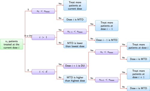
1. Update cumulative number of DLTs $m_i$ and total number of patients $n_i$ treated at the current dose. Use the decision table to make a decision:

   	•	if decision is ‘S’ → Step 2
   	•	if decision is ‘D’ or ‘DU’ → Step 3
   	•	if decision is ‘E’ → Step 4

2. The decision is ‘S’, which means stay at current dose level i. If the sample size at current dose level i reaches the maximum allowed, i.e., $n_i=n_{max}$, declare dose i as the MTD; otherwise, treat additional cohort of patients at current dose level i and go to Step 1.

3. The decision is ‘D’ or ‘DU’. The current dose level i is too toxic and we should de-escalte to next lower dose level. Do one of the following:

   	•	If the current dose level is the lowest dose level, then stop the trial and declare the MTD may be lower than the lowest dose level (inconclusive).
   	•	If the current dose level is not the lowest dose, then: if maximum sample size is not reached ($n_{i-1}<n_{max}$), treat additional cohort of patients at dose level at next lower dose level $(i-1)$, set the current dose level to be the next lower dose level, and go to Step 1; otherwise, stop the trial and declare the next lower dose level is the MTD. Additionally, if the decision is ‘DU’, record this dose level as DU and never treat additional patients at the current dose level again.

4. The decision is ‘E’, which means escalate current does level to next higher dose level. Do one of the following:

   	•	If the current dose level is the highest dose level, then: if maximum sample size is not reached ($n_i<n_{max}$), treat additional cohort of patients at current dose level i and go to Step 1; otherwise, stop the trial and declare that the MTD is higher than the highest dose level (inconclusive);
   	•	If the next higher dose level is of status DU, then: if $n_i<n_{max}$, treat additional cohort of patients at current dose i and go to step 1; otherwise stop the trial, the current dose level i is MTD.
   	•	If $n_{i+1}<n_{max}$, treat additional cohort of patients at dose i + 1, set the current dose level to be next higher dose level, and go to step 1; else, the current dose level i is the MTD.

To run simulations to evaluate a decision table for a particular scenario, we simply call dec.sim function in R:

where truep is the vector of true DLT rates, decTable is a decision table, start.level is the starting dose level in the simulation and nsim is the number of simulated trials. In addition to three-stage decision table, dec.sim also allows user-supplied decision table. This decision table can be either a modified table or any decision table from model-based designs. In order to obtain operating characteristics for the design used in simulation including the percentage of selection as the MTD or over the MTD for each dose, the number of patients treated at each dose level, etc, we use S3 method summary to summarise the simulation results:

A sample output is given as below

To visualise simulation results, the simplest way is to use S3 method plot in R. The detailed document can be found in the R documentation after the package is installed on the computer.

4. Simulations

Simulation studies were conducted to evaluate the performance of the new target toxicity design in terms of safety ($p_{\mathrm{MTD}}$), reliability ($p_{\mathrm{true}}$), # of patients and # of DLT defined below:

• $p_{\mathrm{true}}$: probability of selecting the true MTD correctly.

• $p_{\mathrm{MTD}}$: probability of the patients treated at or below the MTD.

• # of patients: average number of patients treated in the trial.

• # of DLTs: average number of patients experienced DLT in the trial.

Therefore, safety is the probability of patients treated at or below the true MTD and reliability is the probability that the true MTD is selected at the end of the trial for a given scenario. In our simulations, the MTD is derived as the dose level at which MTD is selected in Figure 1. If all doses have toxicity rate higher than target toxicity in Figure 1, the true MTD is lower than the lowest dose. If all doses have toxicity rate lower than target toxicity in Figure 1, the true MTD is higher than the highest dose. In these cases, MTD cannot be determined. This is consistent with the real world case that the target toxicity is never achieved.

4.1. Comparison to other designs

In this subsection, we compare the proposed method with ‘3+3’, mTPI, mTPI-2, BOIN (Liu & Yuan, 2015) and CRM. In our simulations, the target toxicity is set to be 0.3. We consider five dose levels in the simulated trials. The starting dose is the lowest dose level, dose 1. The toxicity rates for the simulated scenarios are generated using the probability model in Paoletti et al. (2004). This model generates dose-toxicity relations in a wide variety of situations by controlling the average slope of the toxicity curve around a targeted percentile θ and the variance round the average. The algorithm is summarised in the following three steps.

1. Randomly choose a level, say dose i as the MTD and generate the corresponding toxicity rate $p_i$ around a targeted percentile θ using $p_i=\mathrm{\Phi }(z_i)$, where $\mathrm{\Phi }(\cdot )$ is the cumulative density function of the standard normal distribution, $z_i\sim N({\mathrm{\Phi }}^{-1}(\theta ),{0.1}^2)$.

2. Generate the differences of the toxicity rates between the MTD level and its two adjacent dose levels. Let $z_{i+1}={\mathrm{\Phi }}^{-1}(\theta )+I_{z_i<{\mathrm{\Phi }}^{-1}(\theta )}({\mathrm{\Phi }}^{-1}(\theta )-z_i)+{ϵ}_{i+1}^2,$ $z_{i-1}={\mathrm{\Phi }}^{-1}(\theta )+I_{z_i>{\mathrm{\Phi }}^{-1}(\theta )}(z_i-{\mathrm{\Phi }}^{-1}(\theta ))+{ϵ}_{i+1}^2,$ where $I(\cdot )$ is the indicator function. Then the corresponding toxicity rates are $p_{i+1}=\mathrm{\Phi }(z_{i+1})$ and $p_{i-1}=\mathrm{\Phi }(z_{i-1})$.

3. Generate the differences between the toxicity rates at the remaining levels. $p_{i+j}=\mathrm{\Phi }(z_{i+j})=\mathrm{\Phi }(z_{i+(j-1)}+{ϵ}_{i+j}^2)$ for $i+j\ge i+2$ and $p_{i-j}=\mathrm{\Phi }(z_{i-j})=\mathrm{\Phi }(z_{i-(j+1)}-{ϵ}_{i-j}^2)$ for $i-j\le i-2$.

We draw ε from a normal distribution with mean ${\mathrm{\Phi }}^{-1}(\theta )$ and standard deviation 0.1 and let $\theta =0.25,0.3,0.35$. For each choice of θ, we simulated 200 scenarios. The simulated toxicity curves and their distribution are depicted in Figure 2. The average difference between two levels are around 0.12, 0.09, 0.06 for $\theta =0.25,0.3,0.35$, respectively. For each scenario, we run 1000 simulated trials.

Figure 2. True toxicity curves and their distributions.

Our design shares some features with interval-based designs which also provide decision tables and can be implemented in a transparent way as the traditional 3+3 design. The key difference is interval-based designs are usually based on Bayesian frameworks thus usually more difficult to explain to physician or choose the parameters in their designs. The interval-based designs divide the interval $[0,1]$ into $[0,p_t-{ϵ}_1),[p_t-{ϵ}_1,p_t+{ϵ}_2]$ and $(p_t+{ϵ}_2,1]$ and access the posterior probabilities that the toxicity rate $p_i$ of a dose i falls into three intervals. Interval designs represent the MTD with an interval instead of a single value. $(p_t-{ϵ}_1,p_t+{ϵ}_2)$ is called equivalence interval and when the estimate of the toxicity rate falls into equivalence interval, the corresponding dose is considered equivalent to the MTD. Different interval-based designs use the different decision rules to guide decision making (Ji & Yang, 2017). For mTPI and mTPI-2, we choose ${ϵ}_1={ϵ}_2=0.05$. BOIN uses different parameters called ${\varphi }_1,{\varphi }_2$. We choose ${\varphi }_1=p_t-{ϵ}_1$ and ${\varphi }_2=p_t+{ϵ}_2$. For CRM, we use the R package dfCRM for simulations. We let the number of patients to be used in the next model-based update to be 3 and the maximum sample size of the trial similar to the average number of patients used in other methods. We set the prior MTD at the third dose, so the initial toxicity rate at dose level 3 is 0.3. The initial guess of toxicity probabilities is (0.0617523, 0.1602510, 0.3000000, 0.4530895, 0.5941906) for the five doses, which was generated by the model calibration method described in Lee Cheung (2009).

TT design is chosen as described in Section 2 by letting ${\alpha }_1=0.6$, ${\alpha }_2=0.4$, and ${\alpha }_u=0.1$. For two-stage designs, we compare TT with the traditional ‘3+3’, mTPI, BOIN and CRM. For CRM, we set the sample size to be fixed at 15 to have comparable sample size to other designs. mTPI-2 has exactly the same decision table as our design when ${ϵ}_1={ϵ}_2=0.05$ thus the comparison is omitted here. It is worth noting that any decision table can be written as a special case in our framework. The type I errors can be calculated when the boundaries are given. For example, the traditional ‘3+3’ has left-side type I error ${\alpha }_{11}=0.343$, ${\alpha }_{12}=0.494$ and right-side type I error ${\alpha }_{21}=0.216$, ${\alpha }_{22}=0.506$. For three-stage designs, we compare our TT ‘3+3+6’ design, mTPI, mTPI-2, BOIN and CRM, where the sample size for CRM is set to be 21. We use the Pocock spending function for both two- and three-stage designs. The type 2 error was not specified since the sample size per dose level has been specified. The decision tables are shown in Tables 3 and 4.

Table 3. Decision tables for ‘3+3’ designs (traditional 3+3, TT, mTPI and BOIN).

# of subjects
	3				6
DLTs	3+3	TT	mTPI	BOIN	3+3	TT	mTPI	BOIN
0	E	E	E	E	E	E	E	E
1	S	S	S	D	E	E	E	E
2	D	D	D	D	D	S	S	D
3	D	DU	DU	DU	D	D	S	D
4					D	DU	DU	DU
5					D	DU	DU	DU
6					D	DU	DU	DU

Notes: The target toxicity rate is 0.3. TT ‘3+3’: the actual type I errors at each stage are (1) ${\alpha }_1=0.343$, 0.494; (2) ${\alpha }_2=0.216$, 0.311; (3) ${\alpha }_u=0.027$, 0.079. mTPI: ${ϵ}_1={ϵ}_2=0.05$. BOIN: ${\varphi }_1=0.25$, ${\varphi }_2=0.35$.

Table 4. Decision tables for ‘3+3+6’ designs (TT, mTPI, mTPI-2 and BOIN).

# of subjects
DLTs	3				6				12
	TT	mTPI	mTPI-2	BOIN	TT	mTPI	mTPI-2	BOIN	TT	mTPI	mTPI-2	BOIN
0	E	E	E	E	E	E	E	E	E	E	E	E
1	S	S	S	D	E	E	E	E	E	E	E	E
2	D	D	D	D	S	S	S	D	E	E	E	E
3	DU	DU	DU	DU	D	S	D	D	E	S	S	E
4					DU	DU	DU	DU	S	S	S	D
5					DU	DU	DU	DU	D	D	D	D
6					DU	DU	DU	DU	D	DU	D	D
7									DU	DU	DU	DU
8									DU	DU	DU	DU
9									DU	DU	DU	DU
10									DU	DU	DU	DU
11									DU	DU	DU	DU
12									DU	DU	DU	DU

Notes: The target toxicity rate is 0.3. TT ‘3+3’: the actual type I errors at each stage are (1) ${\alpha }_1=0.343$, 0.494, 0.576; (2) ${\alpha }_2=0.216$, 0.311, 0.36; (3) ${\alpha }_u=0.027$, 0.079, 0.095. mTPI: ${ϵ}_1={ϵ}_2=0.05$. BOIN: ${\varphi }_1=0.25$, ${\varphi }_2=0.35$.

Table 5 summarises the simulation results to compare these four ‘3+3’ designs and CRM in the reliability, safety measures, the average number of patients treated and the average number of DLTs. First, with regard to reliability, for $\theta =0.25$, the TT design outperforms all other four designs; for $\theta =0.3$ and 0.35, TT performs better than interval-based designs but worse than CRM. The traditional ‘3+3’ is similar to mTPI and but BOIN has the lowest reliability, even about 20% lower than TT and mTPI. CRM is the most reliable design but it is wiggly and unstable–higher variance and lower bias comparing to other designs. In fact, the performance of CRM depends on the prior toxicity probabilities associated with the dose levels. CRM usually performs well when the prior estimates is close to the truth. For most scenarios, the TT design increases 2–6% in reliability compared with 3+3 and mTPI designs. Second, BOIN is the safest design among five designs and other four designs are similar in $p_{\mathrm{MTD}}$. Lastly, the average number of patients treated and average number of DLTs are similar among 3+3, TT, mTPI, and CRM. Although BOIN requires fewer patients and there are less DLTs, it is not a good design due to its lowest reliability. Therefore, we conclude TT 3+3 design outperforms other designs overall in a balanced way between reliability and safety under our choice of settings.

Table 5. Comparison of four ‘3+3’ designs and CRM.

		$p_{\mathrm{true}}$	$p_{\mathrm{MTD}}$	# of patients	# of DLTs
	$\theta =0.25$
3+3	Mean	0.450	0.812	15.084	2.707
	Sd	0.090	0.143	3.432	0.631
TT 3+3	Mean	0.499	0.804	14.373	2.612
	Sd	0.079	0.147	3.280	0.602
mTPI(3+3)	Mean	0.472	0.802	14.105	2.561
	Sd	0.077	0.149	3.309	0.585
BOIN	Mean	0.251	0.883	11.137	1.540
	Sd	0.079	0.109	3.253	0.316
CRM	Mean	0.484	0.826	15.000	2.732
	Sd	0.161	0.159	0.000	1.391
	$\theta =0.30$
3+3	Mean	0.279	0.845	13.804	2.897
	Sd	0.089	0.137	3.367	0.294
TT 3+3	Mean	0.343	0.840	13.061	2.761
	Sd	0.101	0.140	3.151	0.273
mTPI(3+3)	Mean	0.340	0.837	12.826	2.709
	Sd	0.095	0.141	3.161	0.257
BOIN	Mean	0.133	0.906	9.004	1.602
	Sd	0.085	0.104	2.430	0.185
CRM	Mean	0.350	0.876	15.000	3.117
	Sd	0.207	0.131	0.000	1.165
	$\theta =0.35$
3+3	Mean	0.264	0.643	11.143	2.935
	Sd	0.178	0.320	2.441	0.079
TT 3+3	Mean	0.268	0.639	10.554	2.798
	Sd	0.106	0.319	2.223	0.067
mTPI(3+3)	Mean	0.261	0.637	10.356	2.740
	Sd	0.096	0.318	2.221	0.061
BOIN	Mean	0.096	0.318	6.831	0.061
	Sd	0.252	0.343	1.331	0.104
CRM	Mean	0.376	0.692	15.000	3.887
	Sd	0.197	0.339	0.000	0.904

Note: The table reports the average and standard deviation of $p_{\mathrm{true}}$, $p_{\mathrm{MTD}}$, number of patients treated and number of DLTs.

Table 6 summarises the comparison of five designs, including four ‘3+3+6’ designs and CRM. Similar results are shown in these simulation experiments. First, with regard to reliability, TT 3+3+6 and mTPI 3+3+6 are more reliable than TT 3+3 and mTPI 3+3. CRM is more reliable but not as stable as other designs. TT 3+3+6 is slightly better than mTPI and mTPI-2. It can be seen the larger difference between reliability of TT 3+3+6 and mTPI/mTPI-2 3+3+6 over BOIN 3+3+6. This shows BOIN is not a good design with current choice of ${\varphi }_1$ and ${\varphi }_2$. TT 3+3+6 design is more reliable than mTPI/mTPI-2 3+3+6. Second, with regard to safety, TT 3+3+6, BOIN and mTPI/mTPI-2 3+3+6 are less safe than their counterpart ‘3+3’ designs due to more patients are treated. The decrease is very reasonable (about 2%). BOIN 3+3+6 is the safest design among the four 3+3+6 designs, but this is due to a significant decrease in reliability and number of patients treated. And TT 3+3+6, mTPI/mTPI-2 3+3+6 have comparable average number of patients treated and average number of DLTs. Lastly, more patients are needed and experienced DLTs as compared to their 3+3 counterpart, as expected. Although CRM performs better than other designs in some scenarios, the computational burden of CRM simulations is considerable in order to understand the operating characteristics. Unlike TT and interval-based designs, one needs to specify proper prior probability of toxicities and proper model to obtain good performance thus not easy to implement or modify the design. Therefore, we conclude TT 3+3+6 design outperforms other designs overall.

Table 6. Comparison of four ‘3+3+6’ designs and CRM.

		$p_{\mathrm{true}}$	$p_{\mathrm{MTD}}$	# of patients	# of DLTs
	$\theta =0.25$
TT	Mean	0.575	0.794	20.922	4.282
	Sd	0.106	0.147	3.264	1.290
mTPI	Mean	0.568	0.791	20.695	4.257
	Sd	0.089	0.147	2.970	1.278
mTPI-2	Mean	0.558	0.808	20.238	4.021
	Sd	0.088	0.139	3.138	1.152
BOIN	Mean	0.244	0.908	15.551	2.108
	Sd	0.082	0.090	4.030	0.470
CRM	Mean	0.553	0.778	21.000	4.477
	Sd	0.162	0.163	0.000	1.648
	$\theta =0.30$
TT	Mean	0.407	0.823	20.551	4.725
	Sd	0.098	0.144	3.589	0.759
mTPI	Mean	0.389	0.830	19.774	4.515
	Sd	0.105	0.140	3.142	0.725
mTPI-2	Mean	0.375	0.841	19.348	4.323
	Sd	0.103	0.135	3.409	0.630
BOIN	Mean	0.122	0.922	12.771	2.222
	Sd	0.079	0.091	3.440	0.253
CRM	Mean	0.372	0.856	21.000	5.053
	Sd	0.280	0.136	0.000	1.416
	$\theta =0.35$
TT	Mean	0.292	0.602	17.888	4.902
	Sd	0.109	0.309	3.483	0.242
mTPI	Mean	0.289	0.621	16.984	4.631
	Sd	0.112	0.313	2.773	0.249
mTPI-2	Mean	0.290	0.629	16.441	4.422
	Sd	0.120	0.316	3.031	0.183
BOIN	Mean	0.222	0.727	9.505	2.296
	Sd	0.270	0.345	2.156	0.101
CRM	Mean	0.310	0.626	21.000	5.801
	Sd	0.250	0.310	0.000	1.128

Note: The table reports the average and standard deviation of $p_{\mathrm{true}}$, $p_{\mathrm{MTD}}$, number of patients treated and number of DLTs.

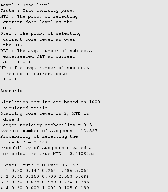
We also present the operating characteristics of TT 3+3 and TT 3+3+6 for three pre-specified dose-toxicity scenarios in Tables 7 and 8. Note that the difference between TT and 3+3, mTPI, mTPI-2, BOIN can be also seen from their decision tables. Each scenario has different location of the MTD level. Since dfCRM uses fixed total number of subjects, we exclude the CRM from the comparison. We summarise the probability that a dose is selected as MTD for two methods: the rule-based approach described in Figure 1 and isotonic regression (Leung & Wang, 2001). Taking the number of patients and number of DLTs at each dose level as input, isotonic regression pools information across doses to estimate MTD. Isotonic estimator has better performance in scenario 1 and comparable performance in scenario 2 and 3 as rule-based estimator for TT designs, but tends to estimate a higher dose level as MTD. Especially in scenario 3, there were cases that, at the end of trial, the decision was to de-escalate the fifth dose level while isotonic regression estimated it as the MTD. On the other hand, isotonic estimator can improve the accuracy for mTPI, mTPI-2 and BOIN. Therefore, based on the limited comparisons, the advantage of the model-based MTD estimation is not evident as its performance varies across designs and scenarios. In practice, a thorough understanding of the operating characteristics is recommended for successful selection of the MTD.

Table 7. Operating characteristics of TT 3+3 under three dose-toxicity scenarios.

	Dose level	1	2	3	4	5
Scenario 1	True toxicity	0.050	0.300	0.500	0.600	0.700
3+3	Selection(%)-1	0.536	0.387	0.050	0.001	0.000
	Selection(%)-2	0.272	0.578	0.142	0.007	0.001
	# of DLTs	0.233	1.510	1.062	0.180	0.014
	# of patients (N = 12.3)	4.803	5.130	2.097	0.285	0.021
TT 3+3	Selection(%)-1	0.319	0.531	0.131	0.013	0.000
	Selection(%)-2	0.259	0.573	0.154	0.013	0.000
	# of DLTs	0.213	1.484	1.129	0.185	0.022
	# of patients (N = 11.7)	4.218	4.989	2.232	0.309	0.030
mTPI 3+3	Selection(%)-1	0.218	0.537	0.224	0.017	0.000
	Selection(%)-2	0.232	0.563	0.188	0.016	0.000
	# of DLTs	0.191	1.391	1.169	0.180	0.005
	# of patients (N = 11.4)	3.975	4.842	2.307	0.288	0.006
BOIN 3+3	Selection(%)-1	0.612	0.226	0.025	0.003	0.000
	Selection(%)-2	0.322	0.550	0.119	0.007	0.002
	# of DLTs	0.223	1.023	0.515	0.104	0.009
	# of patients (N = 9.5)	4.848	3.456	1.083	0.177	0.015
Scenario 2	True toxicity	0.100	0.150	0.300	0.450	0.500
3+3	Selection(%)-1	0.182	0.406	0.241	0.045	0.000
	Selection(%)-2	0.167	0.324	0.367	0.116	0.025
	# of DLTs	0.445	0.686	1.177	0.759	0.175
	# of patients (N = 14.5)	4.206	4.563	3.774	1.686	0.357
TT 3+3	Selection(%)-1	0.134	0.329	0.351	0.123	0.011
	Selection(%)-2	0.154	0.308	0.374	0.132	0.029
	# of DLTs	0.407	0.633	1.051	0.744	0.182
	# of patients (N = 13.7)	3.945	4.176	3.579	1.680	0.363
mTPI 3+3	Selection(%)-1	0.121	0.303	0.360	0.145	0.027
	Selection(%)-2	0.153	0.321	0.357	0.132	0.036
	# of DLTs	0.379	0.610	1.067	0.733	0.167
	# of patients (N = 13.2)	3.828	4.017	3.486	1.602	0.348
BOIN 3+3	Selection(%)-1	0.294	0.308	0.100	0.008	0.000
	Selection(%)-2	0.326	0.359	0.252	0.053	0.010
	# of DLTs	0.396	0.482	0.548	0.216	0.021
	# of patients (N = 9.3)	3.909	3.162	1.713	0.468	0.060
Scenario 3	True toxicity	0.010	0.100	0.250	0.300	0.400
3+3	Selection(%)-1	0.115	0.387	0.263	0.151	0.000
	Selection(%)-2	0.034	0.232	0.400	0.191	0.143
	# of DLTs	0.025	0.505	1.128	0.808	0.448
	# of patients (N = 16.4)	3.405	4.698	4.524	2.607	1.182
TT 3+3	Selection(%)-1	0.034	0.269	0.320	0.247	0.050
	Selection(%)-2	0.032	0.239	0.338	0.253	0.138
	# of DLTs	0.031	0.438	1.049	0.791	0.493
	# of patients (N = 15.4)	3.177	4.257	4.188	2.664	1.203
mTPI 3+3	Selection(%)-1	0.035	0.225	0.340	0.239	0.087
	Selection(%)-2	0.035	0.239	0.338	0.240	0.148
	# of DLTs	0.035	0.442	1.056	0.705	0.455
	# of patients (N = 14.9)	3.201	4.128	4.056	2.418	1.125
BOIN 3+3	Selection(%)-1	0.263	0.437	0.200	0.050	0.000
	Selection(%)-2	0.064	0.341	0.396	0.154	0.045
	# of DLTs	0.043	0.417	0.706	0.375	0.101
	# of patients (N = 12.2)	3.789	4.242	2.844	1.113	0.261

Notes: Selection (%): probability of selection current dose level as the MTD (1- MTD estimated via algorithm in Figure 1; 2- MTD estimated via isotonic regression); # of DLTs: number of DLTs at current dose level; # of patients: number of patients treated at current dose level; N: total number of treated patients. The target toxicity rate is 0.3.

Table 8. Operating characteristics of TT 3+3+6 design under three dose-toxicity scenarios.

	Dose level	1	2	3	4	5
Scenario 1	Toxicity rate	0.050	0.300	0.500	0.600	0.700
TT 3+3+6	Selection(%)-1	0.373	0.532	0.085	0.003	0.000
	Selection(%)-2	0.264	0.613	0.116	0.007	0.000
	# of DLTs	0.322	2.534	1.765	0.299	0.045
	# of patients (N = 19.0)	6.336	8.565	3.552	0.525	0.060
mTPI 3+3+6	Selection(%)-1	0.358	0.551	0.081	0.002	0.000
	Selection(%)-2	0.243	0.613	0.135	0.009	0.000
	# of DLTs	0.272	2.616	1.907	0.302	0.011
	# of patients (N = 19.3)	6.132	8.928	3.840	0.471	0.015
mTPI-2 3+3+6	Selection(%)-1	0.419	0.500	0.070	0.003	0.000
	Selection(%)-2	0.252	0.629	0.113	0.005	0.001
	# of DLTs	0.338	2.546	1.539	0.264	0.013
	# of patients (N = 18.5)	6.642	8.385	3.030	0.450	0.021
BOIN 3+3+6	Selection(%)-1	0.648	0.199	0.003	0.000	0.000
	Selection(%)-2	0.314	0.589	0.095	0.002	0.000
	# of DLTs	0.439	1.429	0.595	0.089	0.000
	# of patients (N = 14.7)	8.613	4.818	1.158	0.144	0.000
Scenario 2	Toxicity rate	0.100	0.150	0.300	0.450	0.500
TT 3+3+6	Selection(%)-1	0.107	0.353	0.392	0.079	0.007
	Selection(%)-2	0.120	0.299	0.425	0.127	0.026
	# of DLTs	0.489	1.070	2.075	1.410	0.302
	# of patients (N = 22.1)	4.827	6.783	6.849	3.102	0.594
mTPI 3+3+6	Selection(%)-1	0.119	0.361	0.375	0.079	0.011
	Selection(%)-2	0.117	0.290	0.444	0.127	0.022
	# of DLTs	0.484	0.995	2.047	1.359	0.308
	# of patients (N = 21.5)	4.797	6.369	6.708	3.006	0.696
mTPI-2 3+3+6	Selection(%)-1	0.108	0.377	0.401	0.063	0.001
	Selection(%)-2	0.131	0.305	0.425	0.108	0.029
	# of DLTs	0.473	0.968	2.102	1.170	0.207
	# of patients (N = 21.0)	4.734	6.600	6.852	2.496	0.411
BOIN 3+3+6	Selection(%)-1	0.297	0.319	0.090	0.005	0.000
	Selection(%)-2	0.328	0.339	0.272	0.050	0.009
	# of DLTs	0.571	0.805	0.737	0.270	0.038
	# of patients ($N=$13.8)	5.700	5.052	2.379	0.588	0.081
Scenario 3	Toxicity rate	0.010	0.100	0.250	0.300	0.400
TT 3+3+6	Selection(%)-1	0.037	0.263	0.297	0.242	0.025
	Selection(%)-2	0.028	0.192	0.343	0.268	0.169
	# of DLTs	0 .035	0.604	1.705	1.569	0.807
	# of patients(N = 23.3)	3.420	6.030	6.702	5.127	2.028
mTPI 3+3+6	Selection(%)-1	0.025	0.231	0.310	0.281	0.051
	Selection(%)-2	0.043	0.191	0.357	0.257	0.152
	# of DLTs	0.030	0.490	1.648	1.429	0.860
	# of patients (N = 22.6)	3.306	5.436	6.729	5.049	2.163
mTPI-2 3+3+6	Selection(%)-1	0.038	0.278	0.328	0.239	0.028
	Selection(%)-2	0.033	0.223	0.343	0.269	0.132
	# of DLTs	0.042	0.617	1.653	1.361	0.677
	# of patients (N = 22.1)	3.462	5.964	6.627	4.491	1.635
BOIN 3+3+6	Selection(%)-1	0.285	0.471	0.138	0.054	0.000
	Selection(%)-2	0.067	0.369	0.364	0.154	0.046
	# of DLTs	0.046	0.715	0.880	0.400	0.124
	# of patients (N = 17.8)	5.553	7.128	3.474	1.404	0.312

Notes: Selection(%): probability of selection current dose level as the MTD (1- MTD estimated via algorithm in Figure 1; 2- MTD estimated via isotonic regression); # of DLTs: number of DLTs at current dose level; # of patients: number of patients treated at current dose level; N: total number of treated patients. The target toxicity rate is 0.3.

4.2. Simulation studies to show power

The following simulation was conducted to investigate the impact of the maximum sample size per dose level of TT designs on the power to detect excessive toxicity. A dose level is considered as over the MTD when the decision is to de-escalate (‘D’ or ‘DU’) at the the end of the trial. We use the probability of selecting each dose level as over the MTD to evaluate the power of the designs. The true toxicity rates for five dose levels are 0.2, 0.3, 0.4, 0.5, 0.6. The target is 0.3, so the MTD is dose 2. In Table 9, we summarise the results on the probability of selecting a dose level as the MTD and over the MTD and the average number of patients treated at each dose level. First, TT ‘3+3+6’ design outperforms TT ‘3+3’ design with a higher probability of correctly selecting Dose Level 2 as MTD, and with lower probability in selecting other dose levels as MTD. Second, TT ‘3+3+6’ design outperforms TT ‘3+3’ design with lower probability in wrongly selecting Dose Level 2 as over MTD, and with higher probability in selecting other dose levels as over MTD. Lastly, more subjects are needed by TT ‘3+3+6’ design as expected. The addition of more subjects improves the power of the trial. The power of TT ‘3+3’ design and TT ‘3+3+6’ design are 0.767 and 0.850, respectively.

Table 9. Comparison of TT ‘3+3’ and TT ‘3+3+6’.

		Prob. MTD		Over MTD		# of Patients
Dose level	Truth	3+3	3+3+6	3+3	3+3+6	3+3	3+3+6
1	0.20	0.373	0.324	0.141	0.156	4.608	6.912
2	0.30	0.307	0.369	0.514	0.480	3.477	6.552
3	0.40	0.148	0.125	0.821	0.849	1.698	3.477
4	0.50	0.026	0.024	0.969	0.974	0.501	1.032
5	0.60	0.002	0.000	1.000	1.000	0.075	0.132

Notes: Truth: true toxicity rate; Prob. MTD: the probability of selecting current dose level as the MTD; Over MTD: the probability of selecting current dose level as over the MTD; # of Patients: the average number of subjects treated at the current dose level.

5. Summary and discussion

We have proposed and analysed a new phase I dose-finding method. Our method depends on user-provided one left-side type I error and two right-side type I errors and a chosen alpha-spending method. The decision rule may be altered via different settings of these parameters and method to achieve goals such as escalating dose level faster or the opposite. The new method is an up-and-down design which is intuitive and doesn't involve complicated calculations. A potential disadvantage is difficult to choose proper type I errors and sample size – but since we show that our TT ‘3+3’ design outperforms other designs in simulations, the design with overall left-side type I error 0.494, overall right-side type I errors of 0.311 are at least safer and more reliable than the widely used classical ‘3+3’ design. Moreover, the traditional ‘3+3’ design is just a special case with overall left-side type I error 0.494 and right-side type I error of 0.506 in the hypothesis testing framework.

We made the comparison of TT designs with other interval-based designs and CRM. For interval-based deisngs, such as mTPI or mTPI-2 designs, a practical and natural question is: are these designs just for one-by-one entry, i.e., entering one patient at a time, once this patient's DLT evaluation has been performed, then entering another patient? If that is the case, then it will take a long time to complete a trial. Additionally, it raises some statistical concerns as it is well known that more stages (corresponding to more interim analyses in a trial) will cause inflation of type I and type II errors.

The decision tables of the proposed TT design is based on a group-sequential framework. However, since the dose-finding process is up-and-down and the trial can come back to a dose even if the dose had an escalation or de-escalation before. The exact left and right side type I errors are not as specified. These left and right-side type I errors are impacted by dose levels studied, toxicity profile and at which dose we start the trial. Therefore, simulation has to be performed to assess the operational characteristics of a design.

One of the biggest advantages of TT design is its transparency. The decision table is clear and easy to use. The new design is based on a statistical hypothesis testing framework. It's easy to understand by statisticians and clinicians as well. The concept of the maximum number of patients needed at each dose level is introduced by associating it with the reliability of selecting MTD correctly and the probability to conclude dose levels over MTD. It will overcome the difficulty in convincing medical community in adding more patients at the dose-finding stage.

We have also provided a software for dose-finding simulations to compare different designs. While the simulation schema was formulated with a different stopping criteria where the maximum sample size equals to number of doses × maximum sample size of each dose, the general result is much more widely applicable; in particular, it applies to other dose-finding methods that provide decision table, such as mTPI, CCD, etc.

Acknowledgments

The authors are very grateful to two anonymous referees for their helpful comments.

Disclosure statement

No potential conflict of interest was reported by the author(s).

References

- Cheung, Y. K. (2013). dfcrm: Dose-finding by the continual reassessment method (Version, 0.2–2.1).
- Cheung, Y. K., & Chappell, R. (2000). Sequential designs for phase I clinical trials with late-onset toxicities. Biometrics, 56(4), 1177–1182. https://doi.org/10.1111/j.0006-341X.2000.01177.x
- Goodman, S. N., Zahurak, M. L., & Piantadosi, S. (1995). Some practical improvements in the continual reassessment method for phase I studies. Statistics in Medicine, 14(11), 1149–1161. https://doi.org/10.1002/(ISSN)1097-0258
- Guo, W., Wang, S.-J., Yang, S., Lynn, H., & Ji, Y. (2017). A Bayesian interval dose-finding design addressing Ockham's razor: mTPI-2. Contemporary Clinical Trials, 58, 23–33. https://doi.org/10.1016/j.cct.2017.04.006
- Ivanova, A., Flournoy, N., & Chung, Y. (2007). Cumulative cohort design for dose-finding. Journal of Statistical Planning and Inference, 137(7), 2316–2327. https://doi.org/10.1016/j.jspi.2006.07.009
- Jennison, C., & Turnbull, B. W. (2000). Group sequential methods with applications to clinical trials. Chapman and Hall.
- Ji, Y., Li, Y., & Nebiyou Bekele, B. (2007). Dose-finding in phase I clinical trials based on toxicity probability intervals. Clinical Trials, 4(3), 235–244. https://doi.org/10.1177/1740774507079442
- Ji, Y., Liu, P., Li, Y., & Nebiyou Bekele, B. (2010). A modified toxicity probability interval method for dose-finding trials. Clinical Trials, 7(6), 653–663. https://doi.org/10.1177/1740774510382799
- Ji, Y., & Yang, S. (2017). On the interval-based dose-finding designs. arXiv:1706.03277.
- Lee, S. M., & Y. K. Cheung (2009). Model calibration in the continual reassessment method. Clinical Trials, 6(3), 227–238. https://doi.org/10.1177/1740774509105076
- Leung, D. H.-Y., & Wang, Y.-G. (2001). Isotonic designs for phase I trials. Controlled Clinical Trials, 22(2), 126–138. https://doi.org/10.1016/s0197-2456(00)00132-x
- Liu, S., & Yuan, Y. (2015). Bayesian optimal interval designs for phase I clinical trials. Journal of the Royal Statistical Society: Series C (Applied Statistics), 64(3), 507–523. https://doi.org/10.1111/rssc.2015.64.issue-3
- O'Brien, P. C., & Fleming, T. R. (1979). A multiple testing procedure for clinical trials. Biometrics, 35(3), 549–556. https://doi.org/10.2307/2530245
- O'Quigley, J., Pepe, M., & Fisher, L. (1990). Continual reassessment method: A practical design for phase 1 clinical trials in cancer. Biometrics, 46(1), 33–48. https://doi.org/10.2307/2531628
- Paoletti, X., O'Quigley, J., & Maccario, J. (2004). Design efficiency in dose finding studies. Computational Statistics & Data Analysis, 45(2), 197–214. https://doi.org/10.1016/S0167-9473(02)00323-7
- Reiner, E., Paoletti, X., & O'Quigley, J. (1999). Operating characteristics of the standard phase i clinical trial design. Computational Statistics & Data Analysis, 30(3), 303–315. https://doi.org/10.1016/S0167-9473(98)00095-4
- Storer, B. E. (2001). An evaluation of phase I clinical trial designs in the continuous dose-response setting. Statistics in Medicine, 20(16), 2399–2408. https://doi.org/10.1002/(ISSN)1097-0258
- Yuan, Y., Hess, K. R., Hilsenbeck, S. G., & Gilbert, M. R. (2016). Bayesian optimal interval design: A simple and well-performing design for phase I oncology trials. Clinical Cancer Research, 22(17), 4291–4301. https://doi.org/10.1158/1078-0432.CCR-16-0592