New extreme value theory for maxima of maxima

Abstract

Although advanced statistical models have been proposed to fit complex data better, the advances of science and technology have generated more complex data, e.g., Big Data, in which existing probability theory and statistical models find their limitations. This work establishes probability foundations for studying extreme values of data generated from a mixture process with the mixture pattern depending on the sample length and data generating sources. In particular, we show that the limit distribution, termed as the accelerated max-stable distribution, of the maxima of maxima of sequences of random variables with the above mixture pattern is a product of three types of extreme value distributions. As a result, our theoretical results are more general than the classical extreme value theory and can be applicable to research problems related to Big Data. Examples are provided to give intuitions of the new distribution family. We also establish mixing conditions for a sequence of random variables to have the limit distributions. The results for the associated independent sequence and the maxima over arbitrary intervals are also developed. We use simulations to demonstrate the advantages of our newly established maxima of maxima extreme value theory.

Keywords:

• maximum domain of attraction
• max-stable distribution
• competing-maximum domain of attractions
• accelerated max-stable distribution
• accelerated extreme value distribution

1. Introduction

Rigorous risk analysis helps to make better decisions and prevent great failures. Extreme value theory has been a powerful tool in risk analysis and is widely applied to risk analysis in finance, insurance, health, climate, and environmental studies. In classical extreme value theory, the sequence of data is assumed to have the same marginal distribution, and the limit distribution of the maxima is in one of the extreme value types if it exists. Galambos (1978), de Haan (1993), Beirlant et al. (2004), de Haan and Ferreira (2006), Leadbetter et al. (2012) and Resnick (2013) amongst many monographs are good literatures introducing the theoretical results in the classical extreme value theory. Mikosch et al. (1997), Embrechts et al. (1999), McNeil and Frey (2000), Coles (2001), Finkenstädt and Rootzén (2004), Castillo et al. (2005), Salvadori et al. (2007) and Dey and Yan (2016) introduce many applications of extreme value method to the areas of science, engineering, nature, finance, insurance and climate. For example, in financial applications, extreme value theory is one of the tools to calculate the Value-at-Risk (VaR) and Expected Shortfall (ES) (e.g., Rocco, 2014; Tsay, 2005). Chavez-Demoulin et al. (2016) offer an extreme value theory (EVT)-based statistical approach for modelling operational risk and losses, by taking into account dependence of the parameters on covariates and time. Zhang and Smith (2010) propose the multivariate maxima of moving maxima (M4) processes and apply the method to model jumps in returns in multivariate financial time series and predict the extreme co-movements in price returns. Daouia et al. (2018) use the extreme expectiles to measure VaR and marginal expected shortfall. In the statistical inference of maximum likelihood estimation (MLE), a discussion on the properties of maximum likelihood estimators of the parameters in generalised extreme value (GEV) distribution was given by Smith (1985). In the paper, it is shown that the classical properties of the MLE hold when the shape parameter $\xi >-1/2$, but not when $\xi \le -1/2$. Bücher and Segers (2017) give a general result on the asymptotic normality of the maximum likelihood estimator for parametric models whose support may depend on the parameters.

In the age of Big Data, the advances of science and technology have been changing data generating processes in a more complex way. As a result, the data structures and dependence structures accompanied by the collected data can be very different from the existed assumptions in many commonly used models. In the literature, advanced statistical models and machine learning approaches have been proposed to fit such complex data or learn the underlying structures better. For example, the support vector machine, the deep learning method, and the random forest method have now been very well recognised and wildly used in data analysis. In extreme value analysis for more complex data, the same marginal distribution assumption and its derived extreme value distributions can be very restrictive and lack of data fitting power. Although statistical models, e.g., Heffernan et al. (2007), Naveau et al. (2011), Tang et al. (2013), Malinowski et al. (2015), Zhang and Zhu (2016) and Idowu and Zhang (2017), have been proposed to model extreme values observed from different data sources with different populations and max-domains of attraction, their probability foundations have not been established.

The definition of the classical maximum domain of attraction cannot be applied directly to the extreme values of data drawn from different populations mixed together. Note that we are not dealing with mixtures of distributions that may belong to a maximum domain of attraction of classical extreme value distribution. In this study, we are dealing with maxima of maxima in which the maxima resulted from each population has its limit extreme value distribution and norming and centering constants and convergence rate. For example, in many real-world applications, the risks one is exposed to usually come from different resources, and the risk at a given time is decided by the dominant one, i.e., not the added risk of all risks. Let us consider a specific example: Suppose a patient suffers two severe diseases. The risk of that the patient will die over a certain time may be best described by the maximum, not the sum, of two risk variables.

This work extends the definition of the maximum domain of attraction to maxima of maxima of sequences of random variables in which the mixing patterns change along with the sample size. The accelerated max-stable distribution (accelerated extreme value distribution) is expressed as a product of the classical extreme value distributions for the maxima of maxima resulted from different distributions. Some basic properties and theoretical results are provided. It can be seen that the classical extreme value distributions are special cases of our newly established family of accelerated max-stable distributions. The results obtained can be applied to more complex data, e.g., Big Data. The new results also establish the probability foundation of previously proposed statistical models in extreme time series modeling. Those models include Heffernan et al. (2007) that introduces one scheme where the maxima are taken over random variables with different distributions, and Zhang and Zhu (2016) that models intra-daily maxima of high-frequency financial data.

The structure of this paper is as follows. In Section 2, (1) we give a brief review of the classical extreme value theory; (2) we define our maxima of maxima of sequences of random variables; (3) we use examples to demonstrate the characteristics of the maxima of maxima; (4) we establish the convergence of maxima of maxima to the accelerated max-stable distributions; (5) we illustrate density functions of the new family of accelerated max-stable distributions and evaluate moments and tail equivalence. Simulations are used to demonstrate the advantages of the accelerated max-stable distribution family in terms of the estimation accuracy of high quantiles at different levels. We also apply this new accelerated max-stable distribution to the high quantiles of the daily maxima of 330 stock returns of S&P 500 companies. In Section 3, the convergence of joint probability for general thresholds and approximation errors are developed. In Section 4, theoretical results for weakly dependent sequences are derived. Section 6 concludes. Additional figures and technical proofs are included in the Appendix.

2. Accelerated max-stable distribution for independent sequences

2.1. A brief review of classical univariate extreme value theory

In classical extreme value theory, the central result is the Fisher-Tippett theorem which specifies the form of the limit distribution for centered and normalised maxima. Let $X_1,X_2,\dots ,X_n$ be a sequence of independent and identically distributed (i.i.d.) non-degenerate random variables (rvs) with common distribution function F and $M_n=max(X_1,\dots ,X_n)$ be the sample maxima. The Fisher-Tippett theorem states that: If for some norming constants $a_n>0$ and centering constants $b_n$ we have (1) $P(a_n(M_n-b_n)\le x)\stackrel{w}{\to }H\left(x\right)$(1) for some nondegenerate H, where $\stackrel{w}{\to }$ stands for convergence in distribution, then H belongs to one type of the following three cumulative distribution functions (cdf's): (2) $\begin{array}{rl}& \mathrm{F}\mathrm{r}\text{'}\mathrm{e}\mathrm{c}\mathrm{h}\mathrm{e}\mathrm{t}:{\mathrm{\Phi }}_{\alpha }\left(x\right)=\left\{\begin{array}{ll}0,& x\le 0\\ \exp \{-x^{-\alpha }\},& x>0,\end{array}\right.\alpha >0.\\ & \mathrm{W}\mathrm{e}\mathrm{i}\mathrm{b}\mathrm{u}\mathrm{l}\mathrm{l}:{\mathrm{\Psi }}_{\alpha }\left(x\right)=\left\{\begin{array}{ll}\exp \{-(-x{)}^{\alpha }\},& x\le 0\\ 1,& x>0,\end{array}\right.\alpha >0.\\ & \mathrm{G}\mathrm{u}\mathrm{m}\mathrm{b}\mathrm{e}\mathrm{l}:\mathrm{\Lambda }\left(x\right)=\exp \{-{\text{e}}^{-x}\},x\in \mathbb{R}.\end{array}$(2) Conversely, every extreme value distribution in (2(2) $\begin{array}{rl}& \mathrm{F}\mathrm{r}\text{'}\mathrm{e}\mathrm{c}\mathrm{h}\mathrm{e}\mathrm{t}:{\mathrm{\Phi }}_{\alpha }\left(x\right)=\left\{\begin{array}{ll}0,& x\le 0\\ \exp \{-x^{-\alpha }\},& x>0,\end{array}\right.\alpha >0.\\ & \mathrm{W}\mathrm{e}\mathrm{i}\mathrm{b}\mathrm{u}\mathrm{l}\mathrm{l}:{\mathrm{\Psi }}_{\alpha }\left(x\right)=\left\{\begin{array}{ll}\exp \{-(-x{)}^{\alpha }\},& x\le 0\\ 1,& x>0,\end{array}\right.\alpha >0.\\ & \mathrm{G}\mathrm{u}\mathrm{m}\mathrm{b}\mathrm{e}\mathrm{l}:\mathrm{\Lambda }\left(x\right)=\exp \{-{\text{e}}^{-x}\},x\in \mathbb{R}.\end{array}$(2) ) can be a limit in (1(1) $P(a_n(M_n-b_n)\le x)\stackrel{w}{\to }H\left(x\right)$(1) ), and in particular, when H itself is the cdf of each $X_i$, the limit is itself. We say that F belongs to the maximum domain of attraction of the extreme value distribution of H, and denote as $F\in \mathrm{M}\mathrm{D}\mathrm{A}\left(H\right)$ when (1(1) $P(a_n(M_n-b_n)\le x)\stackrel{w}{\to }H\left(x\right)$(1) ) holds. H is also called the max-stable distribution since for any $n=2,3,\dots$, there are constants $a_n>0$ and $b_n$ such that $H^n(a_{n}x+b_n)=H\left(x\right)$. Due to this property, the equivalence of extreme value distribution or max-stable distribution in practice is mutually implied.

2.2. Maxima of maxima

Suppose that the independent mixed sequence of random variables $\{X_i{\}}_{i=1}^n$ is composed of k subsequences $\{X_{j,i}{\}}_{i=1}^{n_j},j=1,2,\dots ,k$; $\left\{X_{j,i}{\}}_{i=1}^{n_j}\stackrel{\mathrm{i}.\mathrm{i}.\mathrm{d}.}{\sim }{F}_j\right(x)$, $n_j\to \mathrm{\infty }$ as $n\to \mathrm{\infty }$ and $n=n_1+\cdots +n_k$. Denote $M_{j,n_j}=max(X_{j,i},i=1,\dots ,n_j)$ as the maximum of the jth subsequence, $j=1,2,\dots ,k$. Suppose $F_j\in \mathrm{M}\mathrm{D}\mathrm{A}\left(H_j\right)$, where $H_j$ is one of the three types of extreme value distributions, i.e., $M_{j,n_j}$ has the following limit distribution with some norming constants $a_{j,n_j}>0$ and centering constants $b_{j,n_j},$ (3) $\underset{n\to \mathrm{\infty }}{lim}P\left(a_{j,n_j}\right(M_{j,n_j}-b_{j,n_j})\le x)=H_j\left(x\right).$(3) Define $M_n=max(M_{1,n_1},M_{2,n_2},\dots ,M_{k,n_k})$, i.e., $M_n$ is the maxima of k maxima of $M_{j,n_j}$s. Throughout the paper, $M_n$ is termed as the maxima of maxima. Questions can be asked: (1) whether or not Equation (1(1) $P(a_n(M_n-b_n)\le x)\stackrel{w}{\to }H\left(x\right)$(1) ) holds with appropriately chosen norming constants $a_n>0,b_n$; (2) if Equation (1) holds, whether or not $a_n>0,b_n$ are equivalent to any of $a_{j,n_j}>0,b_{j,n_j}$; (3) whether or not $H\left(x\right)$ is a function of $H_j\left(x\right)$; (4) if all Equations (1)–(3) hold, which one is the best method to be used in practice. This paper intends to answer these four questions.

Practical examples related to the above defined process can be numerous. For example, (1) the maximum temperature of the US in a day can be described by the maximum of maxima of regional maximum temperatures. In each region, the maximum temperature is the maximum temperature recordings among all weather stations in the region. Considering the regions' spatial and geographical patterns, the regional maxima certainly follow different extreme value distributions from one region to another region. The US temperature maxima are the maxima of regional maxima, and should be modelled by a distribution function that is a function of the regional extreme value distribution functions. (2) Considering the daily risk of high-frequency trading in a stock market, one can partition the data into hourly data (from 9:00 am to 4:00 pm). Suppose each hourly maxima $M_{j,n_j}$ of negative returns can be approximately modelled by an extreme value distribution of $H_j\left(x\right)$. It is clear that $M_n$ is better modelled by a function of $H_j\left(x\right),j=1,\dots ,7,$ i.e., not a single $H_j\left(x\right)$. We use the following simple example with k = 2 to illustrate the idea.

Example 2.1

The sequence $\{X_i{\}}_{i=1}^n$ is generated by $X_i=max(Y_i,Z_i)$, where $\left\{Y_i{\}}_{i=1}^n\stackrel{\mathrm{i}.\mathrm{i}.\mathrm{d}.}{\sim }{F}_1\right(x)$, $\left\{Z_i{\}}_{i=1}^n\stackrel{\mathrm{i}.\mathrm{i}.\mathrm{d}.}{\sim }{F}_2\right(x)$, and $F_1\left(x\right)$ and $F_2\left(x\right)$ are two distribution functions. Assume $Y_i$ and $Z_i$ are independent. Then $\left\{X_i{\}}_{i=1}^n\stackrel{\mathrm{i}.\mathrm{i}.\mathrm{d}.}{\sim }F\right(x)=F_1(x\left)F_2\right(x)$.

Remark

The form $X_i=max(Y_i,Z_i)$ is the simplest case in the general mixture models introduced in Zhao and Zhang (2018). It is also the simplest case in the copula structured M4 models studied by Zhang and Zhu (2016).

For illustrative purpose of Example 2.1, let's consider two scenarios. Suppose $\left\{Y_i^{\left[k\right]}{\}}_{i=1}^n\stackrel{\mathrm{i}.\mathrm{i}.\mathrm{d}.}{\sim }N\right(0,1)$ and $\left\{Z_i^{\left[k\right]}{\}}_{i=1}^n\stackrel{\mathrm{i}.\mathrm{i}.\mathrm{d}.}{\sim }U\right[a,b]$ for $k=1,\dots ,m$. Here $U[a,b]$ represents the uniform distribution on the interval $[a,b]$. The superscript $\left[k\right]$ stands for the kth sample sequence. In Scenario 1, Figure 1 illustrates two different simulated sequences of $\{X_i^{\left[k\right]}{\}}_{i=1}^n$, where $X_i^{\left[k\right]}=max(Y_i^{\left[k\right]},Z_i^{\left[k\right]})$, and the maxima of $M_n^{\left[k\right]}=max(X_1^{\left[k\right]},\dots ,X_n^{\left[k\right]})$ for n = 100 and a particular k, e.g., k = 1. Next, we repeatedly generate $m=\mathrm{10,000}$ such sequences $\{X_i^{\left[k\right]}{\}}_{i=1}^n,k=1,\dots ,m$. By taking the maxima $M_n^{\left[k\right]}=max(X_1^{\left[k\right]},\dots ,X_n^{\left[k\right]}),k=1,\dots ,m$, the histogram of $\{M_n^{\left[k\right]}{\}}_{k=1}^m$ is displayed in Figure 2(a) with a = −2.2 and b = 2.2. In Scenario 2, by replacing the marginal distribution of $Z_i^{\left[k\right]}$ with $U[-2.8,2.8]$, the histogram of $M_n^{\left[k\right]}$ is shown in Figure 2(b). It is clear that although $\{X_i^{\left[k\right]}{\}}_{i=1}^n$ is independent and identically distributed (i.i.d.), one can see that the distribution of $M_n$ looks quite different from the three types of extreme value distributions.

Figure 1. Simulated mixed sequences from normal and uniform distributions and their maxima (marked with black dots). In (a), the maximum is from the uniform distribution; in (b), the maximum is from $N(0,1)$.

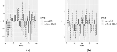
Figure 2. (a) Histogram of $M_n$ from $N(0,1)$ and $U[-2.2,2.2]$. (b) Histogram of $M_n$ from $N(0,1)$ and $U[-2.8,2.8]$.

In Example 2.1, the larger values of two paired underlying subsequences are observed while the smaller values are covered up by larger ones and are never observed. The sample sizes from the two subsequences are the same. However, in general mixed sequences the ratios of sample sizes from two subsequences $n_1/n_2$ can be any value between 0 and infinity and can vary as the total sample size grows. As a result, we can see many kinds of different patterns different from Figure 2.

In practice, data generating processes are naturally formed spatially and temporarily from underlying physical processes of studies. Here we provide two data generating processes in simulation.

1. For a given sample size n, we set the numbers $n_1$ and $n_2$ satisfying $n_1+n_2=n$ and assume that $\underset{n\to \mathrm{\infty }}{lim}{n}_1/(n_1+n_2)\to r$, $r\in (0,1)$. Then we generate the specified $n_1$ and $n_2$ observations from two populations respectively, stack them in a sequence, and perform a random permutation of the combined sequence. In a physical process, the procedure can be designed as: we mix $n_1$ yellow balls and $n_2$ white balls in a bag. Then we draw balls sequentially. If a yellow ball is drawn, generate a number from the first population, otherwise from the second population.

2. Alternatively, suppose $a_{1,n_1}$, $a_{2,n_2}$ are norming constants defined in Equation (3(3) $\underset{n\to \mathrm{\infty }}{lim}P\left(a_{j,n_j}\right(M_{j,n_j}-b_{j,n_j})\le x)=H_j\left(x\right).$(3) ) with known population distributions in simulation, we can set $n_1+n_2=n$ and let $\underset{n\to \mathrm{\infty }}{lim}{a}_{1,n_1}/a_{2,n_2}=r$, and then solve $n_1$ and $n_2$ to generate the observations as the last step.

Example 2.2

Using the sampling scheme designed above. Suppose there are two sequences $\left\{X_{1,i}{\}}_{i=1}^{n_1}\stackrel{\mathrm{i}.\mathrm{i}.\mathrm{d}.}{\sim }N\right(0,0.9)$ and $\left\{X_{2,i}{\}}_{i=1}^{n_2}\stackrel{\mathrm{i}.\mathrm{i}.\mathrm{d}.}{\sim }U\right[-2,2]$ with $n_1=100$ and $n_2=200$. $\{X_k{\}}_{k=1}^{300}$ is mixed with these two sequences. Let $M_n^{\left[j\right]}$ be the maxima of the jth realisation of the sequence, $j=1,\dots ,m$, n = 300. With $m=\mathrm{10,000}$, $\{M_n^{\left[j\right]}{\}}_{j=1}^m$ are calculated and the histogram is shown in Figure 3(a). The case of $n_1=200$ and $n_2=100$ is shown in Figure 3(b).

Figure 3. Histograms of combinations of $M_n$ from $N(0,0.9)$ and $U[-2,2]$. (a) $n_1=100$, $n_2=200$. (b) $n_1=200$, $n_2=100$.

The histograms in Figure 3 look different from any of the three types of extreme value distributions discussed in (2(2) $\begin{array}{rl}& \mathrm{F}\mathrm{r}\text{'}\mathrm{e}\mathrm{c}\mathrm{h}\mathrm{e}\mathrm{t}:{\mathrm{\Phi }}_{\alpha }\left(x\right)=\left\{\begin{array}{ll}0,& x\le 0\\ \exp \{-x^{-\alpha }\},& x>0,\end{array}\right.\alpha >0.\\ & \mathrm{W}\mathrm{e}\mathrm{i}\mathrm{b}\mathrm{u}\mathrm{l}\mathrm{l}:{\mathrm{\Psi }}_{\alpha }\left(x\right)=\left\{\begin{array}{ll}\exp \{-(-x{)}^{\alpha }\},& x\le 0\\ 1,& x>0,\end{array}\right.\alpha >0.\\ & \mathrm{G}\mathrm{u}\mathrm{m}\mathrm{b}\mathrm{e}\mathrm{l}:\mathrm{\Lambda }\left(x\right)=\exp \{-{\text{e}}^{-x}\},x\in \mathbb{R}.\end{array}$(2) ). One feature is that they can be bimodal. On the other hand, the classical GEV distributions are all unimodal. Figure 3 shows two specific examples of choices of $n_1$ and $n_2$. In more general situations, the ratios of $n_1$ and $n_2$ can be any values in $(0,\mathrm{\infty })$. The ratio $n_1/n_2$ may also change as n increases. In Figures 2 and 3, the left parts of the distributions are dominated by the Weibull type induced by the uniform distribution, and the right parts resemble the Gumbel type induced by the normal distribution. The reason is that when we look at the maxima of $\{X_i{\}}_{i=1}^n$, there are two populations competing with each other. Taking (b) in Figure 3 as an example, the winners from $U[-2,2]$ form the steep peak on the left; and the winners from $N(0,0.9)$ form the smoother peak on the right.

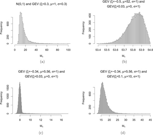
Figure 4(a) shows the distribution of $M_n$ for the sequence which is mixed with $N(0,1)$ and a Fréchet distribution. In (b), (c) and (d), they show the combinations of one Fréchet distribution and one Weibull distribution. Notice that in panel (b), the distribution looks left-skewed and is very similar to a Weibull distribution. However, with the effect of the Fréchet distribution, it actually has an infinite right endpoint.

Figure 4. Histograms of $M_n$. (a) $N(0,1)$ and Fréchet combination. (b)–(d) Some combinations of Fréchet and Weibull.

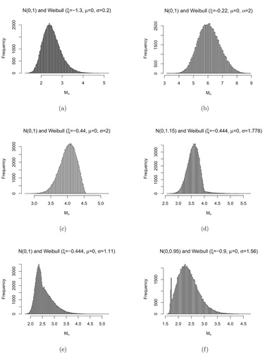
In Figure 5, histograms of $M_n$ are created such that the independent sequences of random variables $\{X_i{\}}_{i=1}^n$ are generated by comparing the pairs of observations from normal and Weibull distribution. They can be unimodal or bimodel, left-skewed or right-skewed. If we use the GEV family to characterise the distributions of $M_n$ in these examples, it may not capture the shape of the distribution properly. For example, if we look at the left part of the distribution in Figure 5(d), it resembles a Weibull distribution that has a finite right endpoint. However, because of the effect of the normal distribution on the right tail, the shape changes suddenly to be similar to a Gumbel distribution with infinite right endpoint. If we fit a GEV distribution to $M_n$, the left part with more sample data may have a large effect on the fitted distribution and we may underestimate the long tail on the right.

Figure 5. Histograms of $M_n$, with combinations of normal distribution and Weibull distribution.

2.3. Convergence to the accelerated max-stable distribution

Throughout the paper, $x_F=sup\{x;F(x)<1\}$ is the right endpoint of a cdf F and let $\overline{F}\left(x\right)=1-F\left(x\right)$; $M_n=max(M_{1,n_1},\dots ,M_{k,n_k})$ is restricted to k = 2. For k>2, relative results can be derived with additional notations. The following theorem shows that under certain conditions on the norming constants $a_{j,n_j}$ and $b_{j,n_j}$, we can choose one set of the norming constants for the global maximum $M_n=max(M_{1,n_1},M_{2,n_2})$ to derive its limit distribution. Theorem 2.1 can be directly derived from Khintchine's theorem.

Theorem 2.1

If $M_{1,n_1}$ and $M_{2,n_2}$ satisfy (3(3) $\underset{n\to \mathrm{\infty }}{lim}P\left(a_{j,n_j}\right(M_{j,n_j}-b_{j,n_j})\le x)=H_j\left(x\right).$(3) ) for j = 1, 2, the limit distribution of $M_n$ as $n\to \mathrm{\infty }$ can be determined in the following cases:

Case 1.	If $\frac{a_{1,n_1}}{a_{2,n_2}}\to a>0$, $a_{1,n_1}(b_{2,n_2}-b_{1,n_1})\to b<+\mathrm{\infty }$, for some constants a and b, then (4) $P\left(a_{2,n_2}\right(M_n-b_{2,n_2})\le x)\to H_1(ax+b)H_2\left(x\right).$(4)
Case 2.	If $\frac{a_{1,n_1}}{a_{2,n_2}}\to 0$, $a_{1,n_1}(b_{2,n_2}-b_{1,n_1})\to +\mathrm{\infty }$, then (5) $P\left(a_{2,n_2}\right(M_n-b_{2,n_2})\le x)\to H_2\left(x\right).$(5)

Notice that the limit in Case 1 is the product of two extreme value distributions, $H_1(ax+b)H_2\left(x\right)$. Although it is in the product form, sometimes it can still be reduced to the three classical extreme value distributions. For example, $\exp \{-x^{-\alpha }\}\exp \{-(\frac{x}{2}{)}^{-\alpha }\}$ is still a Fréchet type. However, in some situations, when the conditions in Case 1 are satisfied, the limit product form cannot be reduced to any one of the three extreme value distributions. We next present several examples to illustrate these possibilities.

Example 2.3

Fréchet and Gumbel

Suppose $F_1\left(x\right)={\mathrm{\Phi }}_{\alpha }\left(x\right)$ is a Fréchet distribution function, and $F_2\left(x\right)=\mathrm{\Lambda }\left(x\right)$ is the standard Gumbel distribution function. By choosing $a_{1,n_1}=n_1^{-1/\alpha },b_{1,n_1}=0$, $a_{2,n_2}=1,b_{2,n_2}=\log n_2$ we have (6) $P(M_{2,n_2}-\log n_2\le x)\to \mathrm{\Lambda }\left(x\right).$(6) Then when $n_1^{1/\alpha }/\log n_2\to \mathrm{\infty }$, we have $\begin{array}{rl}& P(n_1^{-1/\alpha }{M}_n\le x)\\ & =P(n_1^{-1/\alpha }{M}_{1,n_1}\le x,M_{2,n_2}-\log n_2\\ & \le n_1^{1/\alpha }x-\log n_2)\\ & \to {\mathrm{\Phi }}_{\alpha }\left(x\right).\end{array}$

Example 2.4

Fréchet and Fréchet

Suppose $F_1\left(x\right)={\mathrm{\Phi }}_{{\alpha }_1}\left(x\right)$ and $F_2\left(x\right)={\mathrm{\Phi }}_{{\alpha }_2}\left(x\right)$ are two Fréchet distribution functions such that ${\alpha }_1>{\alpha }_2$, which means that the tail of $F_2\left(x\right)$ is heavier than the tail of $F_1\left(x\right)$. By choosing norming constants $a_{1,n_1}=n_1^{-1/{\alpha }_1}$, $b_{1,n_1}=0$ and $a_{2,n_2}=n_2^{-1/{\alpha }_2}$, $b_{2,n_2}=0$ we have (7) $P(n_j^{-1/{\alpha }_j}{M}_{j,n_j}\le x)={\mathrm{\Phi }}_{{\alpha }_j}\left(x\right),j=1,2,$(7) and (8) $\begin{array}{rl}& P(n_2^{-1/{\alpha }_2}{M}_n\le x)\\ & =P\left(n_1^{-1/{\alpha }_1}{M}_{1,n_1}\le \frac{n_2^{1/{\alpha }_2}}{n_1^{1/{\alpha }_1}}x,n_2^{-1/{\alpha }_2}{M}_{2,n_2}\le x\right).\end{array}$(8) If $n_2^{1/{\alpha }_2}/n_1^{1/{\alpha }_1}\to a>0$, then (9) $P(n_2^{-1/{\alpha }_2}{M}_n\le x)\to {\mathrm{\Phi }}_{{\alpha }_1}\left(ax\right){\mathrm{\Phi }}_{{\alpha }_2}\left(x\right).$(9) If $n_2^{1/{\alpha }_2}/n_1^{1/{\alpha }_1}\to +\mathrm{\infty }$, then (10) $P(n_2^{-1/{\alpha }_2}{M}_n\le x)\to {\mathrm{\Phi }}_{{\alpha }_2}\left(x\right).$(10)

In Example 2.4, the sequence is mixed with two Fréchet distributions with different shape parameters. The limit distribution of $M_n$ for this mixed sequence is the product of two Fréchet distributions, which is different from any of the three types of extreme value distributions.

Example 2.5

Uniform and normal

Suppose $F_1\left(x\right)$ is the function of the uniform distribution $U[0,1]$, $F_2\left(x\right)$ is the distribution function of $N(0,1)$. By choosing (11) $a_{1,n_1}=n_1,b_{1,n_1}=1,$(11) and $\begin{array}{rl}{a}_{2,n_2}& =(2\log n_2{)}^{1/2},\\ b_{2,n_2}& =(2\log n_2{)}^{1/2}\\ & -\frac{1}{2}(2\log n_2{)}^{-1/2}(\log \log n_2+\log 4\pi ),\end{array}$we have (12) $P\left(n_1\right(M_{1,n_1}-1)\le x)\to {\text{e}}^x$(12) for x<0, and (13) $P\left(a_{2,n_2}\right(M_{2,n_2}-b_{2,n_2})\le x)\to \mathrm{\Lambda }\left(x\right).$(13) Then $\begin{array}{rl}& P\left(a_{2,n_2}\right(M_n-b_{2,n_2})\le x)\\ & =P\left(n_1(M_{1,n_1}-1)\le n_1\left(\frac{x}{a_{2,n_2}}+b_{2,n_2}-1\right),\right.\\ & \left.a_{2,n_2}(M_{2,n_2}-b_{2,n_2})\le x\phantom{\frac{x}{a_{2,n_2}}}\right).\end{array}$Since $n_1(\frac{x}{a_{2,n_2}}+b_{2,n_2}-1)\to +\mathrm{\infty }$ for any x, we have (14) $P\left(a_{2,n_2}\right(M_n-b_{2,n_2})\le x)\to \mathrm{\Lambda }\left(x\right).$(14)

Example 2.6

Weibull and Weibull

Suppose $x_F<\mathrm{\infty }$ and $K_1>0,K_2>0$, (15) $\begin{array}{r}{F}_1\left(x\right)=1-K_1(x_F-x{)}^{{\alpha }_1},x_F-K_1^{-1/{\alpha }_1}\le x\le x_F,\end{array}$(15) (16) $\begin{array}{r}{F}_2\left(x\right)=1-K_2(x_F-x{)}^{{\alpha }_2},x_F-K_2^{-1/{\alpha }_2}\le x\le x_F,\end{array}$(16) are two polynomial functions with common finite endpoint $x_F$, ${\alpha }_1>{\alpha }_2$. We can choose $a_{1,n_1}=(n_1{K}_1{)}^{1/{\alpha }_1}$, $b_{1,n_1}=x_F$, $a_{2,n_2}=(n_2{K}_2{)}^{1/{\alpha }_2}$, $b_{2,n_2}=x_F$, and (17) $\begin{array}{rl}P\left(\right(n_1{K}_1{)}^{1/{\alpha }_1}(M_{1,n_1}-x_F)\le x)& \to {\mathrm{\Psi }}_{{\alpha }_1}\left(x\right),\end{array}$(17) (18) $\begin{array}{rl}P\left(\right(n_2{K}_2{)}^{1/{\alpha }_2}(M_{2,n_2}-x_F)\le x)& \to {\mathrm{\Psi }}_{{\alpha }_2}\left(x\right).\end{array}$(18) If $\frac{(n_2{K}_2{)}^{1/{\alpha }_2}}{(n_1{K}_1{)}^{1/{\alpha }_1}}\to a>0$, then $\begin{array}{rl}& P\left(\right(n_1{K}_1{)}^{1/{\alpha }_1}(M_n-x_F)\le x)\\ & =P\left(\phantom{\frac{(n_2{K}_2{)}^{1/{\alpha }_2}}{(n_1{K}_1{)}^{1/{\alpha }_1}}}\left(n_1{K}_1{)}^{1/{\alpha }_1}\right(M_{1,n_1}-x_F),(n_2{K}_2{)}^{1/{\alpha }_2}\right.\\ & \times \left.(M_{2,n_2}-x_F)\le \frac{(n_2{K}_2{)}^{1/{\alpha }_2}}{(n_1{K}_1{)}^{1/{\alpha }_1}}x\right)\\ & \to {\mathrm{\Psi }}_{{\alpha }_1}\left(x\right){\mathrm{\Psi }}_{{\alpha }_2}\left(ax\right).\end{array}$

Example 2.7

Normal and Pareto

Suppose $F_1\left(x\right)$ is the standard normal distribution function of $N(0,1)$, $F_2\left(x\right)=1-K{x}^{-\alpha }$, $\alpha >0$, K>0 is a Pareto distribution function. Let $\begin{array}{rl}{a}_{1,n_1}& =(2\log n_1{)}^{1/2},\\ b_{1,n_1}& =(2\log n_1{)}^{1/2}\\ & -\frac{1}{2}(2\log n_1{)}^{-1/2}(\log \log n_1+\log 4\pi ),\\ a_{2,n_2}& =(K{n}_2{)}^{-1/\alpha },b_{2,n_2}=0.\end{array}$Then $\begin{array}{rl}& P\left(a_{1,n_1}\right(M_{1,n_1}-b_{1,n_1})\le x,a_{2,n_2}(M_{2,n_2}-b_{2,n_2})\le x)\\ & \to \left\{\begin{array}{ll}0,& x<0,\\ \exp (-{\mathrm{e}}^{-x}-x^{-\alpha }),& x\ge 0.\end{array}\right.\end{array}$Furthermore, if $a_{2,n_2},b_{1,n_1}\to \mathrm{\infty }$, then $P\left(a_{1,n_1}\right(M_n-b_{1,n_1})\le x)\to \exp (-{\mathrm{e}}^{-x}).$

Example 2.8

Cauchy and uniform distribution

$F_1\left(x\right)=\frac{1}{2}+\frac{1}{\pi }{\tan }^{-1}x$ is the standard Cauchy distribution function, and $F_2\left(x\right)=x,0\le x\le 1$, let $\begin{array}{r}\begin{array}{ll}{a}_{1,n_1}=\tan \left(\frac{\pi }{n_1}\right)\sim \frac{\pi }{n_1},& b_{1,n_1}=0,\\ a_{2,n_2}=n_2,& b_{2,n_2}=1.\end{array}\end{array}$Then $\begin{array}{rl}& P\left(\frac{\pi }{n_1}{M}_{1,n_1}\le x,n_2(M_{2,n_2}-1)\le x\right)\\ & \to \left\{\begin{array}{ll}0,& x<0,\\ \exp (-x^{-1}),& x\ge 0,\end{array}\right.\end{array}$and $P\left(a_{1,n_1}\right(M_n-b_{1,n_1})\le x)\to \left\{\begin{array}{ll}0,& x<0,\\ \exp (-x^{-1}),& x\ge 0.\end{array}\right.$

In Example 2.8, the limit distribution for the normalised $M_{1,n_1}$ is 0 when x<0, and the limit distribution for the normalised $M_{2,n_2}$ is 1 when x>0. Thus, the product is the same as the former one.

In Examples 2.3 and 2.5, we showed that when n is sufficiently large (goes to infinity), the distribution of $M_n$ will be dominated by the subsequence whose marginal distribution has a heavier tail. In Examples 2.4 and 2.6, if the ratio $n_2^{1/{\alpha }_2}/n_1^{1/{\alpha }_1}$ converges to a constant, then one subsequence is never dominated by another, and the limit is of the product form that cannot be reduced to a classical extreme value distribution if ${\alpha }_1\ne {\alpha }_2$.

We now introduce the accelerated max-stable distribution (AMSD) or the accelerated extreme value distribution (AEVD). We consider the convergence of the probability related to the normalised maxima $M_{1,n_1}$ and $M_{2,n_2}$ of two subsequences separately. By the relationship $M_n=max(M_{1,n_1},M_{2,n_2})$, we can use the accelerated max-stable distribution to approximate the distribution of $M_n$. The classical extreme value distributions will be special cases in the accelerated max-stable distribution family.

Definition 2.1

Let $H_1\left(x\right)$ and $H_2\left(x\right)$ be two max-stable distribution functions, we call $H\left(x\right)=H_1\left(x\right)H_2\left(x\right)$ the accelerated max-stable distribution (AMSD/AEVD) function, which is the product of two max-stable distribution functions. More generally, we also say that $H\left(x\right)$ belongs to the accelerated max-stable distribution family if it is the product of k max-stable distribution functions, $k\ge 2$.

Remark

If Z follows an accelerated max-stable distribution $H\left(x\right)$, then Z can be expressed as $Z=max(Z_1,\dots ,Z_k)$, where each $Z_i$ follows a max-stable distribution. By taking maxima of $(Z_1,\dots ,Z_k)$, $Z_i$ values are accelerated by other components $Z_j$s to get observed Z values. On the other hand, we have $\begin{array}{rl}& H_1\left(x\right)H_2\left(x\right)\cdots H_k\left(x\right)\\ & \le H_1\left(x\right)H_2\left(x\right)\cdots H_{k-1}\left(x\right)\\ & \le H_1\left(x\right)H_2\left(x\right)\cdots H_{k-2}\left(x\right)\\ & \le \cdots \le H_1\left(x\right)\end{array}$and $\begin{array}{rl}\overline{H_1\left(x\right)H_2\left(x\right)\cdots H_k\left(x\right)}& \ge \overline{H_1\left(x\right)H_2\left(x\right)\cdots H_{k-1}\left(x\right)}\\ & \ge \overline{H_1\left(x\right)H_2\left(x\right)\cdots H_{k-2}\left(x\right)}\\ & \ge \cdots \ge \overline{H_1\left(x\right)},\end{array}$where $\overline{H}\left(x\right)$ stands for the survival function, i.e., $\overline{H_1\left(x\right)H_2\left(x\right)\cdots H_k\left(x\right)}=1-H_1\left(x\right)H_2\left(x\right)\cdots H_k\left(x\right).$The above inequalities may be regarded as accelerated survival rates. This observation motivates us to call the new distribution as the accelerated max-stable (extreme value) distribution. In the view of risk analysis, the systemic risk of Z is accelerated from individual risks of $Z_j$s given a fixed confidence level.

For the independent sequence of random variables $\{X_i{\}}_{i=1}^n$ with two subsequences $\{X_{1,i}{\}}_{i=1}^{n_1}$ and $\{X_{2,i}{\}}_{i=2}^{n_2}$ defined as above, suppose (3(3) $\underset{n\to \mathrm{\infty }}{lim}P\left(a_{j,n_j}\right(M_{j,n_j}-b_{j,n_j})\le x)=H_j\left(x\right).$(3) ) is satisfied with j = 1, 2 and norming constants $a_{j,n_j}>0,b_{j,n_j}$, i.e., (19) $\underset{n\to \mathrm{\infty }}{lim}P\left(a_{j,n_j}\right(M_{j,n_j}-b_{j,n})\le x)=H_j\left(x\right),j=1,2,$(19) then (20) $\begin{array}{rl}& P(max(a_{1,n_1}(M_{1,n_1}-b_{1,n_1}),a_{2,n_2}(M_{2,n_2}-b_{2,n_2}))\le x)\\ & \to H\left(x\right)=H_1\left(x\right)H_2\left(x\right).\end{array}$(20)

Definition 2.2

Suppose an independent sequence of random variables $\{X_i{\}}_{i=1}^n$ satisfies (19(19) $\underset{n\to \mathrm{\infty }}{lim}P\left(a_{j,n_j}\right(M_{j,n_j}-b_{j,n})\le x)=H_j\left(x\right),j=1,2,$(19) ) and (20(20) $\begin{array}{rl}& P(max(a_{1,n_1}(M_{1,n_1}-b_{1,n_1}),a_{2,n_2}(M_{2,n_2}-b_{2,n_2}))\le x)\\ & \to H\left(x\right)=H_1\left(x\right)H_2\left(x\right).\end{array}$(20) ). We call the underlying distribution, $F_{ni}$, of $X_i$ belongs to the competing-maximum domain of attractions of $H_1$ and $H_2$, and denote as $F_{ni}\in \mathrm{C}\mathrm{M}\mathrm{D}\mathrm{A}(H_1,H_2)$.

We note that a max-stable distribution may also be decomposed into a product of two max-stable distributions. As a result, the max-stable distribution family can be thought as a family that is embedded in the accelerated max-stable distribution family. This observation can be seen in Theorem 2.1 that the limits of $P\left(a_{2,n_2}\right(M_n-b_{2,n_2}\left)\right)$ under two different conditions belong to the accelerated max-stable distribution family. In other words, the accelerated max-stable distributions form an expanded family of distributions that can describe the limiting distribution of the normalised maxima for more general sequences.

For k = 2 and $F_{ni}\in \mathrm{C}\mathrm{M}\mathrm{D}\mathrm{A}(H_1,H_2)$, AMSDs/AEVDs can have the following six possible combinations:

Case 1.	$F_j\in \mathrm{M}\mathrm{D}\mathrm{A}\left(\mathrm{\Lambda }\right),$ j = 1, 2, $\begin{array}{rl}& P\left(a_{1,n_1}\right(M_{1,n_1}-b_{1,n_1})\\ & \le x,a_{2,n_2}(M_{2,n_2}-b_{2,n_2})\le x)\\ & \stackrel{w}{\to }\mathrm{\Lambda }\left(\frac{x-b_1}{a_1}\right)\mathrm{\Lambda }\left(\frac{x-b_2}{a_2}\right).\end{array}$
Case 2.	$F_1\in \mathrm{M}\mathrm{D}\mathrm{A}\left({\mathrm{\Phi }}_{{\alpha }_1}\right)$ and $F_2\in \mathrm{M}\mathrm{D}\mathrm{A}\left({\mathrm{\Phi }}_{{\alpha }_2}\right)$, $\begin{array}{rl}& P\left(a_{1,n_1}\right(M_{1,n_1}-b_{1,n_1})\\ & \le x,a_{2,n_2}(M_{2,n_2}-b_{2,n_2})\le x)\\ & \stackrel{w}{\to }{\mathrm{\Phi }}_{{\alpha }_1}\left(\frac{x-b_1}{a_1}\right){\mathrm{\Phi }}_{{\alpha }_2}\left(\frac{x-b_2}{a_2}\right).\end{array}$
Case 3.	$F_1\in \mathrm{M}\mathrm{D}\mathrm{A}\left({\mathrm{\Psi }}_{{\alpha }_1}\right)$ and $F_2\in \mathrm{M}\mathrm{D}\mathrm{A}\left({\mathrm{\Psi }}_{{\alpha }_2}\right)$, $\begin{array}{rl}& P\left(a_{1,n_1}\right(M_{1,n_1}-b_{1,n_1})\\ & \le x,a_{2,n_2}(M_{2,n_2}-b_{2,n_2})\le x)\\ & \stackrel{w}{\to }{\mathrm{\Psi }}_{{\alpha }_1}\left(\frac{x-b_1}{a_1}\right){\mathrm{\Psi }}_{{\alpha }_2}\left(\frac{x-b_2}{a_2}\right).\end{array}$
Case 4.	$F_1\in \mathrm{M}\mathrm{D}\mathrm{A}\left(\mathrm{\Lambda }\right)$ and $F_2\in \mathrm{M}\mathrm{D}\mathrm{A}\left({\mathrm{\Phi }}_{\alpha }\right)$, $\begin{array}{rl}& P\left(a_{1,n_1}\right(M_{1,n_1}-b_{1,n_1})\\ & \le x,a_{2,n_2}(M_{2,n_2}-b_{2,n_2})\le x)\\ & \stackrel{w}{\to }\mathrm{\Lambda }\left(\frac{x-b_1}{a_1}\right){\mathrm{\Phi }}_{\alpha }\left(\frac{x-b_2}{a_2}\right).\end{array}$
Case 5.	$F_1\in \mathrm{M}\mathrm{D}\mathrm{A}\left(\mathrm{\Lambda }\right)$ and $F_2\in \mathrm{M}\mathrm{D}\mathrm{A}\left({\mathrm{\Psi }}_{\alpha }\right)$, $\begin{array}{rl}& P\left(a_{1,n_1}\right(M_{1,n_1}-b_{1,n_1})\\ & \le x,a_{2,n_2}(M_{2,n_2}-b_{2,n_2})\le x)\\ & \stackrel{w}{\to }\mathrm{\Lambda }\left(\frac{x-b_1}{a_1}\right){\mathrm{\Psi }}_{\alpha }\left(\frac{x-b_2}{a_2}\right).\end{array}$
Case 6.	$F_1\in \mathrm{M}\mathrm{D}\mathrm{A}\left({\mathrm{\Phi }}_{{\alpha }_1}\right)$ and $F_2\in \mathrm{M}\mathrm{D}\mathrm{A}\left({\mathrm{\Psi }}_{{\alpha }_2}\right)$, $\begin{array}{rl}& P\left(a_{1,n_1}\right(M_{1,n_1}-b_{1,n_1})\\ & \le x,a_{2,n_2}(M_{2,n_2}-b_{2,n_2})\le x)\\ & \stackrel{w}{\to }{\mathrm{\Phi }}_{{\alpha }_1}\left(\frac{x-b_1}{a_1}\right){\mathrm{\Psi }}_{{\alpha }_2}\left(\frac{x-b_2}{a_2}\right).\end{array}$

It is easy to see that the classical extreme value distributions are special cases of the AMSD family. For any a>0, b>0 satisfying $\frac{1}{a}+\frac{1}{b}=1,$ we have $\begin{array}{rl}\mathrm{\Lambda }\left(x\right)& =\exp \{-{\mathrm{e}}^{-x}\}=\exp \{-{\mathrm{e}}^{-(\frac{x}{a}+\frac{x}{b})}\}\\ & =\exp \left\{\right(-{\mathrm{e}}^{-x-\log a}-{\mathrm{e}}^{-x-\log b}\left)\right\}\\ & =\mathrm{\Lambda }(x+\log a)\mathrm{\Lambda }(x+\log b).\\ {\mathrm{\Phi }}_{\alpha }\left(x\right)& =\exp \{-x^{-\alpha }\}\\ & =\exp \left\{-{\left(\frac{x}{a^{-\frac{1}{\alpha }}}\right)}^{-\alpha }-{\left(\frac{x}{b^{-\frac{1}{\alpha }}}\right)}^{-\alpha }\right\}\\ & =\mathrm{\Phi }\left(\frac{x}{a^{-\frac{1}{\alpha }}}\right)\mathrm{\Phi }\left(\frac{x}{b^{-\frac{1}{\alpha }}}\right).\\ {\mathrm{\Psi }}_{\alpha }\left(x\right)& =\exp \{-(-x{)}^{\alpha }\}\\ & =\exp \left\{-{\left(\frac{-x}{a^{\frac{1}{\alpha }}}\right)}^{\alpha }-{\left(\frac{-x}{b^{\frac{1}{\alpha }}}\right)}^{\alpha }\right\}\\ & =\mathrm{\Psi }\left(\frac{x}{a^{\frac{1}{\alpha }}}\right)\mathrm{\Psi }\left(\frac{x}{b^{\frac{1}{\alpha }}}\right).\end{array}$Since $H_1\left(x\right)$ and $H_2\left(x\right)$ are max-stable distributions, for any $n_1=2,3,\dots$ and $n_2=2,3,\dots$, there are constants $a_{1,n_1}>0$, $b_{1,n_1}$, $a_{2,n_2}>0$, $b_{2,n_2}$ such that $H_1\left(x\right)H_2\left(x\right)=H_1^{n_1}(a_{1,n_1}x+b_{1,n_1})H_2^{n_2}(a_{2,n_2}x+b_{2,n_2})$.

In Equation (20(20) $\begin{array}{rl}& P(max(a_{1,n_1}(M_{1,n_1}-b_{1,n_1}),a_{2,n_2}(M_{2,n_2}-b_{2,n_2}))\le x)\\ & \to H\left(x\right)=H_1\left(x\right)H_2\left(x\right).\end{array}$(20) ), we considered the convergence of $P(max(a_{1,n_1}(M_{1,n_1}-b_{1,n_1}),a_{2,n_2}(M_{2,n_2}-b_{2,n_2}))\le x),$instead of the traditional $P\left(a_n\right(M_n-b_n)\le x)$. If $n_1$ and $n_2$ are sufficiently large, by (19(19) $\underset{n\to \mathrm{\infty }}{lim}P\left(a_{j,n_j}\right(M_{j,n_j}-b_{j,n})\le x)=H_j\left(x\right),j=1,2,$(19) ) we have $P\left(a_{1,n_1}\right(M_{1,n_1}-b_{1,n_1})\le x)\approx G_1\left(x\right)$ and $P\left(a_{2,n_2}\right(M_{2,n_2}-b_{2,n_2})\le x)\approx G_2\left(x\right)$, then (21) $\begin{array}{rl}P(M_n\le x)& =P(max(M_{1,n_1},M_{2,n_2})\le x)\\ & =P(M_{1,n_1}\le x)P(M_{2,n_2}\le x)\\ & \approx G_1(a_{1,n_1}(x-b_{1,n_1}))G_2(a_{2,n_2}(x-b_{2,n_2}))\\ & =G_1^{\ast }\left(x\right)G_2^{\ast }\left(x\right),\end{array}$(21) where $G_j^{\ast }$ is of the same type as $G_j$, j = 1, 2.

To close this section, we remark that (21(21) $\begin{array}{rl}P(M_n\le x)& =P(max(M_{1,n_1},M_{2,n_2})\le x)\\ & =P(M_{1,n_1}\le x)P(M_{2,n_2}\le x)\\ & \approx G_1(a_{1,n_1}(x-b_{1,n_1}))G_2(a_{2,n_2}(x-b_{2,n_2}))\\ & =G_1^{\ast }\left(x\right)G_2^{\ast }\left(x\right),\end{array}$(21) ) is the basis of applying the newly introduced AMSD/AEVD family to real data. Based on (21(21) $\begin{array}{rl}P(M_n\le x)& =P(max(M_{1,n_1},M_{2,n_2})\le x)\\ & =P(M_{1,n_1}\le x)P(M_{2,n_2}\le x)\\ & \approx G_1(a_{1,n_1}(x-b_{1,n_1}))G_2(a_{2,n_2}(x-b_{2,n_2}))\\ & =G_1^{\ast }\left(x\right)G_2^{\ast }\left(x\right),\end{array}$(21) ), in practice, we don't need to worry about the values of $n_1$, $n_2$, $a_{1,n_1}$, $b_{1,n_1}$, $a_{2,n_2}$, $b_{2,n_2}$, as they are absorbed in $G_1^{\ast }\left(x\right)$ and $G_2^{\ast }\left(x\right)$, see also Coles (2001). In our examples, we have used some fixed numbers for $n_1$ and $n_2$. They are just for simulation convenience. When n tends to infinity, the values of $n_1$ and $n_2$ will depend on n.

The next section presents density functions and shapes from which one can see the flexibility of applying the new distribution to real data modelling.

2.4. Density functions and density plots

The density function of the accelerated max-stable distribution requires some discussion of the support region of the cumulative distribution function. We can express the two terms in the product using the form of the generalised extreme value distribution, (22) $\begin{array}{rl}F\left(x\right)& =H_{{\xi }_1;{\mu }_1,{\sigma }_1}\left(x\right)H_{{\xi }_2;{\mu }_2,{\sigma }_2}\left(x\right)\\ & =\exp \left\{-{\left[1+{\xi }_1\frac{x-{\mu }_1}{{\sigma }_1}\right]}^{-1/{\xi }_1}\right.\\ & \left.-{\left[1+{\xi }_2\frac{x-{\mu }_2}{{\sigma }_2}\right]}^{-1/{\xi }_2}\right\},\end{array}$(22) where $1+{\xi }_1\frac{x-{\mu }_1}{{\sigma }_1}>0$ and $1+{\xi }_2\frac{x-{\mu }_2}{{\sigma }_2}>0$. We include the special case $H_{0;{\mu }_i,{\sigma }_2}$ as the limit of $H_{{\xi }_i;{\mu }_i,{\sigma }_i}$ for ${\xi }_i\to 0,i=1,2$. Denote the density function as $f\left(x\right)$ and let $\begin{array}{rl}h\left(x\right)& =\exp \left\{-{\left[1+{\xi }_1\frac{x-{\mu }_1}{{\sigma }_1}\right]}^{-1/{\xi }_1}\right.\\ & \left.-{\left[1+{\xi }_2\frac{x-{\mu }_2}{{\sigma }_2}\right]}^{-1/{\xi }_2}\right\}\\ & \times \left[\frac{1}{{\sigma }_1}{\left(1+{\xi }_1\frac{x-{\mu }_1}{{\sigma }_1}\right)}^{-1/{\xi }_1-1}\right.\\ & \left.+\frac{1}{{\sigma }_2}{\left(1+{\xi }_2\frac{x-{\mu }_2}{{\sigma }_2}\right)}^{-1/{\xi }_2-1}\right].\end{array}$Since ${\xi }_1$ and ${\xi }_2$ are symmetric, we only present one of them. We have the following six cases for the density functions.

Case 1.	${\xi }_1=0,{\xi }_2=0$. $\begin{array}{rl}f\left(x\right)& =\exp \{-{\mathrm{e}}^{-\frac{x-{\mu }_1}{{\sigma }_1}}-{\mathrm{e}}^{-\frac{x-{\mu }_2}{{\sigma }_2}}\}\\ & \times \left[\frac{1}{{\sigma }_1}{\mathrm{e}}^{-\frac{x-{\mu }_1}{{\sigma }_1}}+\frac{1}{{\sigma }_2}{\mathrm{e}}^{-\frac{x-{\mu }_2}{{\sigma }_2}}\right],x\in \mathbb{R}.\end{array}$
Case 2.	${\xi }_1>0$, ${\xi }_2>0,$ assuming ${\mu }_1-\frac{{\sigma }_1}{{\xi }_1}\ge {\mu }_2-\frac{{\sigma }_2}{{\xi }_2}$, then $f\left(x\right)=\left\{\begin{array}{ll}h\left(x\right),& \mathrm{i}\mathrm{f}x>{\mu }_1-\frac{{\sigma }_1}{{\xi }_1},\\ 0,& \mathrm{i}\mathrm{f}x\le {\mu }_1-\frac{{\sigma }_1}{{\xi }_1}.\end{array}\right.$
Case 3.	${\xi }_1<0$, ${\xi }_2<0$, assuming ${\mu }_1-\frac{{\sigma }_1}{{\xi }_1}\ge {\mu }_2-\frac{{\sigma }_2}{{\xi }_2}$, then $\begin{array}{r}f\left(x\right)=\left\{\begin{array}{ll}h\left(x\right),& \mathrm{i}\mathrm{f}x<{\mu }_2-\frac{{\sigma }_2}{{\xi }_2},\\ \exp \left\{-{\left[1+{\xi }_1\frac{x-{\mu }_1}{{\sigma }_1}\right]}^{-1/{\xi }_1}\right\}\\ \times \left[\frac{1}{{\sigma }_1}{\left(1+{\xi }_1\frac{x-{\mu }_1}{{\sigma }_1}\right)}^{-1/{\xi }_1-1}\right],& \mathrm{i}\mathrm{f}{\mu }_2-\frac{{\sigma }_2}{{\xi }_2}\le x\le {\mu }_1-\frac{{\sigma }_1}{{\xi }_1},\\ 0,& \mathrm{i}\mathrm{f}x>{\mu }_1-\frac{{\sigma }_1}{{\xi }_1}.\end{array}\right.\end{array}$
Case 4.	${\xi }_1=0$, ${\xi }_2>0$. $\begin{array}{r}f\left(x\right)=\left\{\begin{array}{ll}\exp \left\{-{\mathrm{e}}^{-\frac{x-{\mu }_1}{{\sigma }_1}}-{\left[1+{\xi }_2\frac{x-{\mu }_2}{{\sigma }_2}\right]}^{-1/{\xi }_2}\right\},& \\ \times \left[\frac{1}{{\sigma }_1}{\mathrm{e}}^{-\frac{x-{\mu }_1}{{\sigma }_1}}+\frac{1}{{\sigma }_2}(1+{\xi }_2\frac{x-{\mu }_2}{{\sigma }_2}{)}^{-1/{\xi }_2-1}\right],& \mathrm{i}\mathrm{f}x>{\mu }_2-\frac{{\sigma }_2}{{\xi }_2},\\ 0,& \mathrm{i}\mathrm{f}x\le {\mu }_2-\frac{{\sigma }_2}{{\xi }_2}.\end{array}\right.\end{array}$
Case 5.	${\xi }_1=0$, ${\xi }_2<0$. $\begin{array}{r}f\left(x\right)=\left\{\begin{array}{l}\exp \left\{-{\mathrm{e}}^{-\frac{x-{\mu }_1}{{\sigma }_1}}-{\left[1+{\xi }_2\frac{x-{\mu }_2}{{\sigma }_2}\right]}^{-1/{\xi }_2}\right\}\\ \times \left[\frac{1}{{\sigma }_1}{\mathrm{e}}^{-\frac{x-{\mu }_1}{{\sigma }_1}}+\frac{1}{{\sigma }_2}(1+{\xi }_2\frac{x-{\mu }_2}{{\sigma }_2}{)}^{-1/{\xi }_2-1}\right],& \mathrm{i}\mathrm{f}x<{\mu }_2-\frac{{\sigma }_2}{{\xi }_2},\\ \exp \{-{\mathrm{e}}^{-\frac{x-{\mu }_1}{{\sigma }_1}}\}\times \frac{1}{{\sigma }_1}{\mathrm{e}}^{-\frac{x-{\mu }_1}{{\sigma }_1}},& \mathrm{i}\mathrm{f}x\ge {\mu }_2-\frac{{\sigma }_2}{{\xi }_2}.\end{array}\right.\end{array}$
Case 6.	${\xi }_1>0$, ${\xi }_2<0$. If ${\mu }_1-\frac{{\sigma }_1}{{\xi }_1}\ge {\mu }_2-\frac{{\sigma }_2}{{\xi }_2}$, $\begin{array}{r}f\left(x\right)=\left\{\begin{array}{ll}\exp \left\{-{\left[1+{\xi }_1\frac{x-{\mu }_1}{{\sigma }_1}\right]}^{-1/{\xi }_1}\right\}& \\ \times \left[\frac{1}{{\sigma }_1}{\left[1+{\xi }_1\frac{x-{\mu }_1}{{\sigma }_1}\phantom{{}^{-1/{\xi }_1-1}}\right]}^{-1/{\xi }_1-1}\right],& \mathrm{i}\mathrm{f}x>{\mu }_1-\frac{{\sigma }_1}{{\xi }_1},\\ 0,& \mathrm{i}\mathrm{f}x\le {\mu }_1-\frac{{\sigma }_1}{{\xi }_1}.\end{array}\right.\end{array}$If ${\mu }_1-\frac{{\sigma }_1}{{\xi }_1}<{\mu }_2-\frac{{\sigma }_2}{{\xi }_2}$, $\begin{array}{r}f\left(x\right)=\left\{\begin{array}{ll}\exp \left\{-{\left[1+{\xi }_1\frac{x-{\mu }_1}{{\sigma }_1}\right]}^{-1/{\xi }_1}\right\}& \\ \times \left[\frac{1}{{\sigma }_1}{\left[1+{\xi }_1\frac{x-{\mu }_1}{{\sigma }_1}\right]}^{-1/{\xi }_1-1}\right],& \mathrm{i}\mathrm{f}x>{\mu }_2-\frac{{\sigma }_2}{{\xi }_2},\\ h\left(x\right),& \mathrm{i}\mathrm{f}{\mu }_1-\frac{{\sigma }_1}{{\xi }_1}\le x\le {\mu }_2-\frac{{\sigma }_2}{{\xi }_2},\\ 0,& \mathrm{i}\mathrm{f}x<{\mu }_1-\frac{{\sigma }_1}{{\xi }_1}.\end{array}\right.\end{array}$

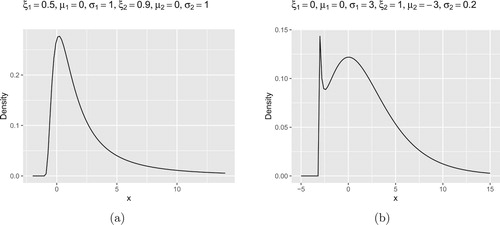
In Figures 6 and 7, four density plots of Weibull-Gumbel type are shown. In Figure 8, panel (a) is the density plot of Fréchet-Fréchet type; and panel (b) is the density plot of Fréchet-Gumbel type. We can observe that they capture the shapes of the histograms shown in Figures 4 and 5.

Figure 6. Density plots of the accelerated max-stable distributions with Weibull-Gumbel combinations. (a) ${\xi }_1=0$, ${\mu }_1=0.5$, ${\sigma }_1=1$, ${\xi }_2=-1$, ${\mu }_2=-1$, ${\sigma }_2=1$. (b) ${\xi }_1=0$, ${\mu }_1=0.5$, ${\sigma }_1=1$, ${\xi }_2=-1$, ${\mu }_2=0.5$, ${\sigma }_2=1$.

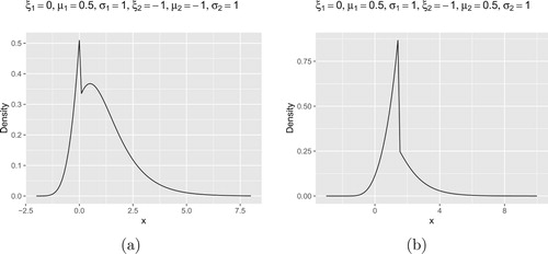
Figure 7. Density plots of the accelerated max-stable distributions with Weibull-Gumbel combinations. (a) ${\xi }_1=-1$, ${\mu }_1=-1$, ${\sigma }_1=1$, ${\xi }_2=0$, ${\mu }_2=0.5$, ${\sigma }_2=0.7$. (b) ${\xi }_1=-0.5$, ${\mu }_1=-2$, ${\sigma }_1=1$, ${\xi }_2=0$, ${\mu }_2=-1$, ${\sigma }_2=0.7$.

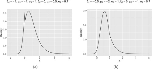
Figure 8. (a) Density plot of the accelerated max-stable distribution with Fréchet-Fréchet combinition. ${\xi }_1=0.5$, ${\mu }_1=0$, ${\sigma }_1=1$, ${\xi }_2=0.9$, ${\mu }_2=0$, ${\sigma }_2=1$. (b) Density plot of the accelerated max-stable distributions with Fréchet-Gumbel combinition. ${\xi }_1=0$, ${\mu }_1=0$, ${\sigma }_1=3$, ${\xi }_2=1$, ${\mu }_2=-3$, ${\sigma }_2=0.2$.

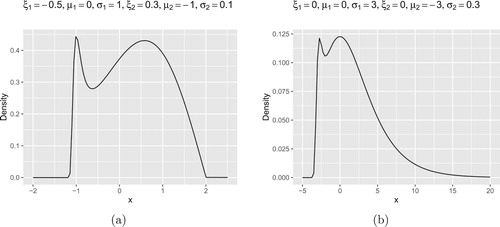
In Figure 9(b), it is for ${\xi }_1={\xi }_2=0$, i.e., the combination of two Gumbel distributions. In this case, the density plot is bimodal, which is different from that of a Gumbel distribution. Suppose that $X_{1,i}\sim N({\mu }_1,{\sigma }_1)$ and $X_{2,j}\sim N({\mu }_2,{\sigma }_2)$, $1\le i\le n_1$ and $1\le j\le n_2$, then we have some norming constants $a_{1,n_1}>0,b_{1,n_1}$ and $a_{2,n_2}>0,b_{2,n_2}$ such that (23) $\begin{array}{rl}& P\left(a_{1,n_1}\right(M_{1,n_1}-b_{1,n_1})\le x,a_{2,n_2}(M_{2,n_2}-b_{2,n_2})\le x)\\ & \to \mathrm{\Lambda }\left(\frac{x-{\mu }_1}{{\sigma }_1}\right)\mathrm{\Lambda }\left(\frac{x-{\mu }_2}{{\sigma }_2}\right)\\ & =\exp \{-{\mathrm{e}}^{-\frac{x-{\mu }_1}{{\sigma }_1}}-{\mathrm{e}}^{-\frac{x-{\mu }_2}{{\sigma }_2}}\}.\end{array}$(23) Here the limit product form requires that the two scale parameters ${\sigma }_1\ne {\sigma }_2$. Otherwise, the product $\exp \{-{\mathrm{e}}^{-\frac{x-{\mu }_1}{\sigma }}-{\mathrm{e}}^{-\frac{x-{\mu }_2}{\sigma }}\}$ reduces to the Gumbel type.

Figure 9. (a) Density plot of the accelerated max-stable distribution with Weibull-Fréchet combination. ${\xi }_1=-0.5$, ${\mu }_1=0$, ${\sigma }_1=1$, ${\xi }_2=0.3$, ${\mu }_2=-1$, ${\sigma }_2=0.1$. (b) Density plot of the accelerated max-stable distribution with Gumbel-Gumbel combinition. ${\xi }_1=0$, ${\mu }_1=0$, ${\sigma }_1=3$, ${\xi }_2=0$, ${\mu }_2=-3$, ${\sigma }_2=0.3$.

2.5. Tail equivalence and the existence of moments

In this section, we discuss some results of tail-equivalence, and which moments are finite for certain AMSDs/AEVDs.

Definition 2.3

Two cdf's F and H are called tail-equivalent if they have the same right endpoint, i.e., if $x_F=x_H$, and (24) $\underset{x\to x_F}{lim}\overline{F}\left(x\right)/\overline{H}\left(x\right)=c$(24) for some constant $0<c<\mathrm{\infty }$.

We have the following facts.

Fact 2.1

It is clear that the product distribution of a Weibull distribution and another type of extreme value distribution $H\left(x\right)$ is tail equivalent to $H\left(x\right)$.

Fact 2.2

Suppose $X\sim {\mathrm{\Phi }}_{{\alpha }_1}{\mathrm{\Phi }}_{{\alpha }_2}$, let ${\mu }_k=E\left(X^k\right)$ be the kth moment of X, then ${\mu }_k$ is finite only if $k<min({\alpha }_1,{\alpha }_2)$.

Suppose ${\alpha }_1<{\alpha }_2$, then ${\mathrm{\Phi }}_{{\alpha }_1}$ has a heavier tail than ${\mathrm{\Phi }}_{{\alpha }_2}$. Let ${\mu }_k^{\left(1\right)}$ be the kth moment of $X\sim {\mathrm{\Phi }}_{{\alpha }_1}$. We know that ${\mu }_k^{\left(1\right)}<\mathrm{\infty }$ only if $k<{\alpha }_1$. This implies that ${\mathrm{\Phi }}_{{\alpha }_1}{\mathrm{\Phi }}_{{\alpha }_2}$ has the same right-tail heaviness as ${\mathrm{\Phi }}_{{\alpha }_1}$.

Fact 2.3

If $0<{\alpha }_1<{\alpha }_2$, then ${\mathrm{\Phi }}_{{\alpha }_1}{\mathrm{\Phi }}_{{\alpha }_2}$ and ${\mathrm{\Phi }}_{{\alpha }_1}$ are tail-equivalent.

Fact 2.4

Suppose $X\sim \mathrm{\Lambda }\left(x\right){\mathrm{\Phi }}_{\alpha }\left(x\right)$. Let ${\mu }_k=E\left(X^k\right)$ be the kth moment of X. Then ${\mu }_k$ is finite only if $k<\alpha$.

Fact 2.5

$\mathrm{\Lambda }\left(x\right){\mathrm{\Phi }}_{\alpha }\left(x\right)$ and ${\mathrm{\Phi }}_{\alpha }\left(x\right)$ are tail-equivalent.

Fact 2.6

If $H_1\left(x\right)$ has a heavier tail than $H_2\left(x\right)$, then the accelerated max-stable distribution $H_1\left(x\right)H_2\left(x\right)$ is tail-equivalent to $H_1\left(x\right)$.

3. Joint convergence and approximation errors

3.1. Convergence of joint probability for general thresholds

It may also be interesting to consider the limits of $P(M_{1,n_1}\le u_{1,n_1},M_{2,n_2}\le u_{2,n_2})$ for some sequences $u_{1,n_1}$ and $u_{2,n_2}$ not necessarily of the form $x/a_{i,n_i}+b_{i,n_i}$ or even not dependent on x. Here $n_1$ and $n_2$ are the lengths of the two subsequences, we may write them specifically as $n_1\left(n\right)$ and $n_2\left(n\right)$ since they vary with the total length n. When choosing $u_{j,n_j}=x/a_{j,n_j}+b_{j,n_j}$ for j = 1, 2, it becomes the problem we discussed before. The question is:

Which conditions on $F_1$ and $F_2$ ensure that the limit of $P(M_{1,n_1}\le u_{1,n_1},M_{2,n_2}\le u_{2,n_2})$ for $n\to \mathrm{\infty }$ exists for appropriate constants $u_{1,n_1}$ and $u_{2,n_2}$?

Some conditions on tails ${\overline{F}}_1$ and ${\overline{F}}_2$ are required to ensure that $P(M_{1,n_1}\le u_{1,n_1},M_{2,n_2}\le u_{2,n_2})$ converges to a non-trivial limit, i.e., a number in $(0,1)$.

Theorem 3.1

Suppose $\{X_i{\}}_{i=1}^n$ is an independent sequence of random variables which is mixed with two subsequences $\{X_{1,i}{\}}_{i=1}^{n_1}$ and $\{X_{2,i}{\}}_{i=1}^{n_2}$ with underlying distributions $F_1\left(x\right)$ and $F_2\left(x\right)$, $n_1\to \mathrm{\infty }$ and $n_2\to \mathrm{\infty }$ as $n\to \mathrm{\infty }$. Let $0\le \tau <\mathrm{\infty }$ and $\{u_{1,i}{\}}_{i=1}^{n_1}$ and $\{u_{2,i}{\}}_{i=1}^{n_2}$ are two sequences of real numbers such that (25) $\begin{array}{rl}& n_1(1-F_1(u_{1,n_1}\left)\right)+n_2(1-F_2(u_{2,n_2}\left)\right)\\ & \to \tau \mathrm{a}\mathrm{s}n\to \mathrm{\infty }.\end{array}$(25) Then (26) $P(M_{1,n_1}\le u_{1,n_1},M_{2,n_2}\le u_{2,n_2})\to {\mathrm{e}}^{-\tau }\mathrm{a}\mathrm{s}n\to \mathrm{\infty }.$(26) Conversely, if (26(26) $P(M_{1,n_1}\le u_{1,n_1},M_{2,n_2}\le u_{2,n_2})\to {\mathrm{e}}^{-\tau }\mathrm{a}\mathrm{s}n\to \mathrm{\infty }.$(26) ) holds for some $0\le \tau <\mathrm{\infty }$, then so does (25(25) $\begin{array}{rl}& n_1(1-F_1(u_{1,n_1}\left)\right)+n_2(1-F_2(u_{2,n_2}\left)\right)\\ & \to \tau \mathrm{a}\mathrm{s}n\to \mathrm{\infty }.\end{array}$(25) ).

Remark

Since $1-F\left(u_{j,n_j}\right)$ is the probability that $X_{j,i}$ exceeds level $u_{j,n_j}$, Equation (25(25) $\begin{array}{rl}& n_1(1-F_1(u_{1,n_1}\left)\right)+n_2(1-F_2(u_{2,n_2}\left)\right)\\ & \to \tau \mathrm{a}\mathrm{s}n\to \mathrm{\infty }.\end{array}$(25) ) means that the expected number of exceedences of $u_{1,n_1}$ by $\{X_{1,i}{\}}_{i=1}^{n_1}$ and $u_{2,n_2}$ by $\{X_{2,i}{\}}_{i=1}^{n_2}$ in total converges to τ. When the sequence is generated from one distribution $F\left(x\right)$, Theorem 3.1 can be reduced to the classical result by choosing $u_{1,n_1}=u_{2,n_2}=u_n$. That is (27) $n(1-F(u_n\left)\right)\to \tau ,$(27) if and only if (28) $P(M_n\le u_n)\to {\mathrm{e}}^{-\tau }$(28) as $n\to \mathrm{\infty }$.

The following corollary gives the conditions such that we can choose one of $\{u_{1,i}{\}}_{i=1}^{n_1}$ and $\{u_{2,i}{\}}_{i=1}^{n_2}$ to be applied to $M_n$, and derive a similar limit of $P(M_n\le u_n)$. The condition involves both the ratio of two tail probabilities $\frac{1-F_1\left(u_{1,n_1}\right)}{1-F_2\left(u_{2,n_2}\right)}$ and $\frac{n_1}{n_2}$.

Corollary 3.1

Let $0\le {\tau }_1<\mathrm{\infty }$, $0\le {\tau }_2<\mathrm{\infty }$. Suppose that there exist two sequences $u_{1,n_1}$ and $u_{2,n_2}$ such that (29) $\begin{array}{rl}{n}_1(1-F_1(u_{1,n_1}\left)\right)& \to {\tau }_1,\\ n_2(1-F_2(u_{2,n_2}\left)\right)& \to {\tau }_2.\end{array}$(29) Then (30) $P(M_{1,n_1}\le u_{1,n},M_{2,n_2}\le u_{2,n})\to {\mathrm{e}}^{-{\tau }_1-{\tau }_2}.$(30) Moreover, if $\frac{n_2(1-F_2(u_{1,n_1}\left)\right)}{n_1(1-F_1(u_{1,n_1}\left)\right)}\to t$, where $0\le t<\mathrm{\infty }$, then (31) $P(M_n\le u_{1,n_1})\to {\mathrm{e}}^{-{\tau }_1(1+t)}.$(31)

Specifically, if we choose $u_{1,n_1}=\frac{x}{a_{1,n_1}}+b_{1,n_1}$, $u_{2,n_2}=\frac{x}{a_{2,n_2}}+b_{2,n_2}$, and suppose that (32) $\begin{array}{rl}P\left(a_{1,n_1}\right(M_{1,n_1}-b_{1,n_1})\le x)& \to G_1\left(x\right),\end{array}$(32) (33) $\begin{array}{rl}P\left(a_{2,n_2}\right(M_{2,n_2}-b_{2,n_2})\le x)& \to G_2\left(x\right),\end{array}$(33) then $G_1$ and $G_2$ belong to the GEV distribution family and the limit in (31(31) $P(M_n\le u_{1,n_1})\to {\mathrm{e}}^{-{\tau }_1(1+t)}.$(31) ) becomes $G_1\left(x\right)G_2\left(x\right)$.

The following is an example of mixed sequence and the limit properties of the maxima of subsequences and the global maxima.

Example 3.1

Suppose $\{X_i{\}}_{i=1}^n$ is a sequence of random variables combining two subsequences $\{X_{1,i}{\}}_{i=1}^{n_1}$ and $\{X_{2,i}{\}}_{i=1}^{n_2}$. Suppose $\frac{n_1}{n}\to p$, where $0\le p\le 1$, $\{X_{1,i}{\}}_{i=1}^{n_1}$ and $\{X_{2,i}{\}}_{i=1}^{n_2}$ are i.i.d. from a Pareto distribution with $F_1\left(x\right)=1-K{x}^{-{\alpha }_1},{\alpha }_1>0,K>0,x>0$ and a Fréchet distribution with $F_2\left(x\right)=\exp (-x^{-{\alpha }_2}),{\alpha }_2>0,x>0,$ respectively.

Since $(1-F_1(tx\left)\right)/(1-F_1(t\left)\right)=x^{-{\alpha }_1}$ for each $x>0,$ so that Type II (Fréchet) limit applies. For $u_{1,n_1}=(K{n}_{1,n_1}/\tau {)}^{1/{\alpha }_1}$ we have $1-F_1\left(u_{1,n_1}\right)=\tau /n_1$, so that (34) $P\left(M_{1,n_1}\le {\left(\frac{K{n}_1}{\tau }\right)}^{1/{\alpha }_1}\right)\to {\mathrm{e}}^{-\tau }.$(34) Putting $\tau =x^{-{\alpha }_1}$ for $x\ge 0$, (35) $P\left(\right(K{n}_1{)}^{-1/{\alpha }_1}{M}_{1,n_1}\le x)\to \exp (-x^{-{\alpha }_1}).$(35) On the other hand, $F_2^{n_2}\left(n_2^{1/{\alpha }_2}x\right)=F_2\left(x\right)$, i.e., $P(n_2^{-1/{\alpha }_2}{M}_{2,n_2}\le x)=F_2\left(x\right)$.

Then we have for $x\ge 0$, (36) $\begin{array}{rl}& P\left(\right(K{n}_1{)}^{-1/{\alpha }_1}{M}_{1,n_1}\\ & \le x,n_2^{-1/{\alpha }_2}{M}_{2,n_2}\le x)\to \exp (-x^{-{\alpha }_1}-x^{-{\alpha }_2}).\end{array}$(36) Since $\begin{array}{rl}\underset{x\to \mathrm{\infty }}{lim}\frac{{\overline{F}}_1\left(x\right)}{{\overline{F}}_2\left(x\right)}& =\underset{x\to \mathrm{\infty }}{lim}\frac{K{x}^{-{\alpha }_1}}{1-\exp (-x^{-{\alpha }_2})}\\ & =\underset{x\to \mathrm{\infty }}{lim}\frac{K{x}^{-{\alpha }_1}}{x^{-{\alpha }_2}+O\left(x^{-2{\alpha }_2}\right)}\\ & \to \left\{\begin{array}{ll}0,& {\alpha }_1>{\alpha }_2,\\ K,& {\alpha }_1={\alpha }_2,\\ \mathrm{\infty },& {\alpha }_1<{\alpha }_2.\end{array}\right.\end{array}$When ${\alpha }_1={\alpha }_2$, the condition $\frac{n_2(1-F_2(u_{1,n_1}\left)\right)}{n_1(1-F_1(u_{1,n_1}\left)\right)}\to \frac{1-p}{pK}$ in Corollary 3.1 is satisfied, hence (37) $P(M_n\le n_1^{-1/{\alpha }_1}x)\to \exp \left(-x^{-{\alpha }_1}\left(1+\frac{1-p}{pk}\right)\right).$(37) Since $n_1\sim np,$ we also have (38) $P(M_n\le (np{)}^{-1/{\alpha }_1}x)\to \exp \left(-x^{-{\alpha }_1}\left(1+\frac{1-p}{pk}\right)\right).$(38)

3.2. Approximation error

The convergence results are usually accompanied by the question of the approximation error. Suppose $n_1(1-F_1(u_{1,n_1}\left)\right)\to {\tau }_1$ and $n_2(1-F_2(u_{2,n_2}\left)\right)\to {\tau }_2$, writing ${\tau }_{1,n_1}=n_1(1-F_1(u_{1,n_1}\left)\right)$ and ${\tau }_{2,n_2}=n_2(1-F_2(u_{2,n_2}\left)\right)$, then by Theorem 3.1 we have (39) $P(M_{1,n_1}\le u_{1,n_1},M_{2,n_2}\le u_{2,n_2})\to {\mathrm{e}}^{-{\tau }_1-{\tau }_2}.$(39) The approximation can be decomposed into several parts. We have ${\left(1-\frac{{\tau }_{1,n_1}}{n_1}\right)}^{n_1}\approx {\mathrm{e}}^{-{\tau }_{1,n_1}},{\left(1-\frac{{\tau }_{2,n_2}}{n_2}\right)}^{n_2}\approx {\mathrm{e}}^{-{\tau }_{2,n_2}},$and ${\mathrm{e}}^{-{\tau }_{1,n_1}}\approx {\mathrm{e}}^{-{\tau }_1},{\mathrm{e}}^{-{\tau }_{2,n_2}}\approx {\mathrm{e}}^{-{\tau }_2}.$We denote $\begin{array}{rl}{\mathrm{\Delta }}_{1,n_1}& ={\left(1-\frac{{\tau }_{1,n_1}}{n_1}\right)}^{n_1}-{\mathrm{e}}^{-{\tau }_{1,n_1}},\\ {\mathrm{\Delta }}_{1,n_1}^{\prime }& ={\mathrm{e}}^{-{\tau }_{1,n_1}}-{\mathrm{e}}^{-{\tau }_1},\\ {\mathrm{\Delta }}_{2,n_2}& ={\left(1-\frac{{\tau }_{2,n_2}}{n_2}\right)}^{n_2}-{\mathrm{e}}^{-{\tau }_{2,n_2}},\\ {\mathrm{\Delta }}_{2,n_2}^{\prime }& ={\mathrm{e}}^{-{\tau }_{2,n_2}}-{\mathrm{e}}^{-{\tau }_2}.\end{array}$Then $\begin{array}{rl}P(M_{1,n_1}\le u_{1,n_1})-{\mathrm{e}}^{-{\tau }_1}& ={\mathrm{\Delta }}_{1,n_1}+{\mathrm{\Delta }}_{1,n_1}^{\prime },\\ P(M_{2,n_2}\le u_{2,n_2})-{\mathrm{e}}^{-{\tau }_2}& ={\mathrm{\Delta }}_{2,n_2}+{\mathrm{\Delta }}_{2,n_2}^{\prime }.\end{array}$The following result gives the bound for the approximation error.

Theorem 3.2

Let $\{X_i{\}}_{i=1}^n$ be an independent sequence of random variables mixed with two subsequences $\{X_{1,i}{\}}_{i=1}^{n_1}$ and $\{X_{2,i}{\}}_{i=1}^{n_2}$, which satisfies $n_1(1-F_1(u_{1,n_1}\left)\right)\to {\tau }_1$ and $n_2(1-F_2(u_{2,n_2}\left)\right)\to {\tau }_2$, ${\mathrm{\Delta }}_{1,n_1}$, ${\mathrm{\Delta }}_{1,n_1}^{\prime },$ ${\mathrm{\Delta }}_{2,n_2},$ ${\mathrm{\Delta }}_{2,n_2}^{\prime }$ are defined as above, then $\begin{array}{rl}P(M_{1,n_1}& \le u_{1,n_1},M_{2,n_2}\le u_{2,n_2})-{\mathrm{e}}^{-{\tau }_1-{\tau }_2}\\ & \le {\mathrm{\Delta }}_{1,n_1}+{\mathrm{\Delta }}_{1,n_1}^{\prime }+{\mathrm{\Delta }}_{2,n_2}+{\mathrm{\Delta }}_{2,n_2}^{\prime }\end{array}$with $\begin{array}{rl}0\le -{\mathrm{\Delta }}_{j,n_j}& \le \frac{{\tau }_{j,n_j}{\mathrm{e}}^{-{\tau }_{j,n_j}}}{2}\cdot \frac{1}{n_j-1}\\ & \le 0.3\cdot \frac{1}{n_j-1},\mathrm{f}\mathrm{o}\mathrm{r}j=1,2,\end{array}$where the first bound is asymptotically sharp, in the sense that if ${\tau }_{j,n_j}\to {\tau }_j$ then ${\mathrm{\Delta }}_{j,n_j}\sim -\left(\frac{{\tau }_j{\mathrm{e}}^{-{\tau }_j}}{2}\right)/n_j$. Furthermore, for ${\tau }_j-{\tau }_{j,n_j}\le \log 2$, ${\mathrm{\Delta }}_{j,n_j}^{\prime }={\mathrm{e}}^{{\tau }_j}\left\{\right({\tau }_j-{\tau }_{j,n_j})+{\theta }_j({\tau }_j-{\tau }_{j,n_j}{)}^2\},$with $0<{\theta }_j<1$.

If ${\tau }_{j,n_j}\to {\tau }_j$ for $u_{j,n_j}=x/a_{j,n_j}+b_{j,n_j}$, then (39(39) $P(M_{1,n_1}\le u_{1,n_1},M_{2,n_2}\le u_{2,n_2})\to {\mathrm{e}}^{-{\tau }_1-{\tau }_2}.$(39) ) holds. By Lemma A.1, (39(39) $P(M_{1,n_1}\le u_{1,n_1},M_{2,n_2}\le u_{2,n_2})\to {\mathrm{e}}^{-{\tau }_1-{\tau }_2}.$(39) ) holds also if $a_{j,n_j}$ and $b_{j,n_j}$ are replaced by different constants ${\alpha }_{j,n_j}$ and ${\text{β}}_{j,n_j}$, satisfying ${\alpha }_{j,n_j}/a_{j,n_j}\to 1$ and $({\text{β}}_{j,n_j}-b_{j,n_j})/a_{j,n_j}\to 0$. However, the speed of convergence to zero of ${\mathrm{\Delta }}_{j,n_j}^{\prime }$ (thus the speed of $P(M_{j,n_j}\le u_{j,n_j})$ to ${\mathrm{e}}^{-{\tau }_j}$) can be very different for different choices of norming constants.

4. Weakly dependent sequences

In this section, we extend the independent sequences to weakly dependent sequences. For a sequence of random variables $\{X_i{\}}_{i=1}^n$ with identical distribution, it is stationary if $\{X_{j_1},\dots ,X_{j_n}\}$ and $\{X_{j_1+m},\dots ,X_{j_n+m}\}$ have the same joint distribution for any choice of n, $j_1,\dots ,j_n$, and m. For the mixed sequence, we will provide some alternatives so that the desired results still hold. We assume that the dependence between $X_{i,k}$ and $X_{i,j}$ falls off in some specific way as $|k-j|$ increases.

4.1. Review of some weakly dependent conditions

Some weakly dependent conditions in the literature can be generalised to the scenarios of mixed sequences. For m-dependent sequence $\{X_i{\}}_{i=1}^n$, $X_i$ and $X_j$ are independent if $|i-j|>m$. Another commonly used condition is the strong mixing condition first introduced by Rosenblatt (1956). A sequence of random variables $\{X_i{\}}_{i=1}^n$ is said to satisfy the strong mixing condition if for some $A\in \mathcal{F}(X_1,\dots ,X_p)$ and $B\in \mathcal{F}(X_{p+k+1},X_{p+k+2},\dots )$ $|P(A\cap B)-P\left(A\right)P\left(B\right)|<g\left(k\right)$for any p and k, where $g\left(k\right)\to 0$ as $k\to \mathrm{\infty }$; $\mathcal{F}\mathcal{(}\cdot \mathcal{)}$ is the σ-field generated by the indicated random variables. The function $g\left(k\right)$ does not depend on the sets A and B, so the strong mixing condition is uniform.

For normal sequences, the correlation between $X_k$ and $X_j$ may be a better measure of dependence. We can also use the dependence restriction $|\mathrm{C}\mathrm{o}\mathrm{r}\mathrm{r}(X_k,X_j)|\le g(|k-j|),$ where $g\left(k\right)\to 0$ as $k\to \mathrm{\infty }$.

Since the event $\{M_n\le u\}$ is the same as $\{X_1\le u,X_2\le u,\dots ,X_n\le u\}$. We may restric the events on this type of event. Following Leadbetter et al. (2012), we use $F_{i_1,\dots ,i_n}\left(u\right)$ to denote $P(X_{i_1}\le u,X_{i_2}\le u,\dots ,X_{i_n}\le u)$. The following condition D is a weakened condition of strong mixing.

The condition $\text{D}$ will be said to hold if for any integers $i_1<\cdots <i_p$ and $j_1<\cdots <j_{p^{\prime }}$ for which $j_1-i_p\ge l$, and any real u, (40) $|F_{i_1,\dots ,i_p,j_1,\dots ,j_{p^{\prime }}}\left(u\right)-F_{i_1,\dots ,i_p}\left(u\right)F_{j_1,\dots ,j_{p^{\prime }}}\left(u\right)|\le g\left(l\right)$(40) where $g\left(l\right)\to 0$ as $l\to \mathrm{\infty }$.

Under the condition D, the Extremal Types Theorem also holds. Since we usually deal with the event $\{M_n\le u_n\}$ for some levels $\left\{u_n\right\}$, the condition can still be weakened. The condition $D\left(u_n\right)$ is defined as follows.

The condition $\mathit{D}\mathit{\left(}{\mathit{u}}_{\mathit{n}}\mathit{\right)}$ will be said to hold if for any integers (41) $1\le i_1<\cdots <i_p<j_1<\cdots <j_{p^{\prime }}\le n$(41) for which $j_1-i_p\ge l$, we have (42) $|F_{i_1,\dots ,i_p,j_1,\dots ,j_{p^{\prime }}}\left(u_n\right)-F_{i_1,\dots ,i_p}\left(u_n\right)F_{j_1,\dots ,j_{p^{\prime }}}\left(u_n\right)|\le {\alpha }_{n,l}$(42) where ${\alpha }_{n,l_n}\to 0$ as $n\to \mathrm{\infty }$ for some sequence $l_n=o\left(n\right)$.

The condition $D\left(u_n\right)$ guarantees that $lim infP(M_n\le u_n)\ge {\mathrm{e}}^{-\tau }$. We still need a further assumption to have the opposite inequality for the upper limit. Here we present the $D^{\prime }\left(u_n\right)$ condition used in Watson (1954) and Loynes (1965). This condition bounds the probability of more than one exceedance among $X_1,\dots ,X_{\left[n/k\right]}$, therefore no multiple points in the point process of exceedances.

The condition $D^{\prime }\left(u_n\right)$ will be said to hold for the sequence of random variables $\{X_i{\}}_{i=1}^n$, if (43) $\underset{n\to \mathrm{\infty }}{lim sup}n\sum _{j=2}^{\left[n/k\right]}P\{X_1>u_n,X_j>u_n\}\to 0$(43) as $k\to \mathrm{\infty }$, (where [ ] denotes the interger part).

If both conditions $D\left(u_n\right)$ and $D^{\prime }\left(u_n\right)$ are satisfied, we have $P(M_n\le u_n)\to {\mathrm{e}}^{-\tau }$ is equivalent to $n(1-F(u_n\left)\right)\to \tau \mathrm{a}\mathrm{s}n\to \mathrm{\infty }$ for $0\le \tau <\mathrm{\infty }$.

4.2. Weakly dependent mixed sequences

To generalise the results from non-mixed sequences to mixed sequences, we need to modify the conditions of $D\left(u_n\right)$ and $D^{\prime }\left(u_n\right)$. We use ${\mathbf{u}}_n$ to denote the vector of levels $(u_{1,n_1},u_{2,n_2})$ when the sequence $\{X_i{\}}_{i=1}^n$ is composed of two subsequences $\{X_{1,i}{\}}_{i=1}^{n_1}$ and $\{X_{2,i}{\}}_{i=2}^{n_2}$, $n_1+n_2=n$. We further assume that $\frac{n_1}{n}\to p$ as $n\to \mathrm{\infty }$, $0\le p\le 1$, so that $\frac{n_2}{n}\to 1-p$.

Before introducing the more general $D\left({\mathbf{u}}_n\right)$ condition, we introduce some new notations. Let $u_n^{\left(i\right)}=u_{1,n_1}I(X_i\in \{X_{1,i}{\}}_{i=1}^{n_1})+u_{2,n_2}I(X_i\in \left\{X_{2,i}{\}}_{i=1}^{n_2}\right)$. Here $I\left(A\right)=1$ indicates that the event A is true, otherwise $I\left(A\right)=0$. The notation $u_n^{\left(i\right)}$ represents the threshold for $X_i$, which depends on the subsequence that $X_i$ belongs to. For example, if $X_1=X_{1,1}$ and $X_2=X_{2,1}$, then $P(X_1\le u_n^{\left(1\right)},X_2\le u_n^{\left(2\right)})$ represents $P(X_{1,1}\le u_{1,n_1},X_{2,1}\le u_{2,n_2})$. After introducing this notation, we can state the condition $D\left({\mathbf{u}}_n\right)$ as follows.

The condition $D\left({\mathbf{u}}_n\right)$ will be said to hold for the mixed sequence of random variables $\{X_i{\}}_{i=1}^n$ with two subsequences $\{X_{1,i}{\}}_{i=1}^{n_1}$ and $\{X_{2,i}{\}}_{i=1}^{n_2}$ if for any integers (44) $1\le i_1<\cdots <i_p<j_1<\cdots <j_{p^{\prime }}\le n$(44) for which $j_1-i_p\ge l$, we have $\begin{array}{rl}& |P(X_{i_1}\le u_n^{\left(i_1\right)},\dots ,X_{i_p}\\ & \le u_n^{\left(i_p\right)},X_{j_1}\le u_n^{\left(j_1\right)},\dots ,X_{j_{p^{\prime }}}\le u_n^{\left(j_{p^{\prime }}\right)})\\ & -P(X_{i_1}\le u_n^{\left(i_1\right)},\dots ,X_{i_p}\le u_n^{\left(i_p\right)})\\ & P(X_{j_1}\le u_n^{\left(j_1\right)},\dots ,X_{j_{p^{\prime }}}\le u_n^{\left(j_{p^{\prime }}\right)})|<{\alpha }_{n,l},\end{array}$where ${\alpha }_{n,l_n}\to 0$ as $n\to \mathrm{\infty }$ for some sequence $l_n=o\left(n\right)$.

Similarly, we can also extend the condition $D^{\prime }\left(u_n\right)$ for mixed sequences, which is denoted as $D^{\prime }\left({\mathbf{u}}_n\right)$.

The condition $D^{\prime }\left({\mathbf{u}}_n\right)$ will be said to hold for the mixed sequence of random variables $\{X_i{\}}_{i=1}^n$ and levels ${\mathbf{u}}_n=(u_{1,n_1},u_{2,n_2})$ if (45) $\begin{array}{rl}& \underset{n\to \mathrm{\infty }}{lim sup}k\sum _{1\le i<j\le \left[n/k\right]}P(X_i>u_n^{\left(i\right)},X_j>u_n^{\left(j\right)})\to 0\\ & \mathrm{a}\mathrm{s}k\to \mathrm{\infty },\end{array}$(45) where $u_n^{\left(i\right)}=u_{1,n_1}I(X_i\in \{X_{1,i}{\}}_{i=1}^{n_1})+u_{2,n_2}I(X_i\in \left\{X_{2,i}{\}}_{i=2}^{n_2}\right),$ and $\left[\right]$ denotes the integer part.

Equation (45(45) $\begin{array}{rl}& \underset{n\to \mathrm{\infty }}{lim sup}k\sum _{1\le i<j\le \left[n/k\right]}P(X_i>u_n^{\left(i\right)},X_j>u_n^{\left(j\right)})\to 0\\ & \mathrm{a}\mathrm{s}k\to \mathrm{\infty },\end{array}$(45) ) means that $\underset{n\to \mathrm{\infty }}{lim sup}\sum _{1\le i<j\le \left[n/k\right]}P(X_i>u_n^{\left(i\right)},X_j>u_n^{\left(j\right)})=o\left(1/k\right)$. It can be observed that if $D\left({\mathbf{u}}_n\right)$ holds for the mixed sequence $\{X_i{\}}_{i=1}^n$, then $D\left(u_{j,n_j}\right)$ also holds for the subsequence $\{X_{j,i}{\}}_{i=1}^{n_j}$, for j = 1, 2. The same conclusion is also true for the condition $D^{\prime }\left({\mathbf{u}}_n\right)$.

After introducing the conditions $D\left({\mathbf{u}}_n\right)$ and $D^{\prime }\left({\mathbf{u}}_n\right)$, we have the extended results for mixed sequences. We assume that the two subsequences $\{X_{1,i}{\}}_{i=1}^{n_1}$ and $\{X_{2,i}{\}}_{i=2}^{n_2}$ are independent with each other. Also, for any interval $I_n$ with $l_n$ members, there are $a_n$ members from $\{X_{1,i}{\}}_{i=1}^{n_1}$ and $b_n$ members from $\{X_{2,i}{\}}_{i=2}^{n_2}$. We assume that the proportion of each subsequence $\frac{a_n}{l_n}\to p$ and $\frac{b_n}{l_n}\to 1-p$, where $0\le p\le 1$.

Theorem 4.1

Let $\{X_i{\}}_{i=1}^n$ be a weakly dependent mixed sequence of random variables with two subsequences $\{X_{1,i}{\}}_{i=1}^{n_1}$ and $\{X_{2,i}{\}}_{i=1}^{n_2}$, with sample size proportions $\frac{n_1}{n}\to p$ and $\frac{n_2}{n}\to 1-p$ as $n\to \mathrm{\infty }$, $0\le p\le 1$. Suppose that $D\left({\mathbf{u}}_n\right)$ and $D^{\prime }\left({\mathbf{u}}_n\right)$ hold for $\{X_i{\}}_{i=1}^n$, then for $0\le \tau <\mathrm{\infty },$ (46) $P(M_{1,n_1}\le u_{1,n_1},M_{2,n_2}\le u_{2,n_2})\to {\mathrm{e}}^{-\tau }$(46) if and only if (47) $n_1(1-F_1(u_{1,n_1}\left)\right)+n_2(1-F_2(u_{2,n_2}\left)\right)\to \tau .$(47)

Based on Theorem 4.1, we have the following corollary.

Corollary 4.1

The same conclusions hold with $\tau =\mathrm{\infty }$ (i.e., $P(M_{1,n_1}\le u_{1,n_1},M_{2,n_2}\le u_{2,n_2})\to 0$ if and only if $n_1(1-F_1(u_{1,n_1}\left)\right)+n_2(1-F_2(u_{2,n_2}\left)\right)\to \mathrm{\infty })$ if the requirements that $D\left({\mathbf{u}}_n\right)$, $D^{\prime }\left({\mathbf{u}}_n\right)$ hold are replaced by the condition that, for arbitrarily large $\tau (<\mathrm{\infty })$, there exists a vector of levels ${\mathbf{v}}_n=(v_{1,n_1},v_{2,n_2})$ such that $v_{1,n_1}>u_{1,n_1},v_{2,n_2}>u_{2,n_2}$, which satisfy $n_1(1-F_1(v_{1,n_1}\left)\right)+n_2(1-F_2(v_{2,n_2}\left)\right)\to \tau$ with $D\left({\mathbf{v}}_n\right)$ and $D^{\prime }\left({\mathbf{v}}_n\right)$ hold.

Theorem 4.1 tells us the property of the joint probability $P(M_{1,n_1}\le u_{1,n_1},M_{2,n_2}\le u_{2,n_2})$ given the tail properties of $F_1$ and $F_2$. $n_1(1-F_1(u_{1,n_1}\left)\right)+n_2(1-F_2(u_{2,n_2}\left)\right)$ is the mean exceedances of the two thresholds by the corresponding subsequences in total. Theorem 4.1 is the generalisation of Theorem 3.1 under the condition that the mixed sequence is weakly dependent within each subsequence.

4.3. Associated independent sequences

The ‘independent sequence associated with $\{X_i{\}}_{i=1}^n$’ can be used to study the maxima of dependent sequence. It was first introduced by Loynes (1965). For a weakly dependent sequence of random variables $\{X_i{\}}_{i=1}^n$, the notation $\{{\hat{X}}_i{\}}_{i=1}^n$ is used to be the independent sequence with the same marginal distribution as $\{X_i{\}}_{i=1}^n$, and write ${\hat{M}}_n=max({\hat{X}}_1,\dots ,{\hat{X}}_n)$. When $\{X_i{\}}_{i=1}^n$ is mixed with two subsequences $\{X_{1,i}{\}}_{i=1}^{n_1}$ and $\{X_{2,i}{\}}_{i=1}^{n_2}$ with different marginal distributions, we still have the associated independent subsequences $\{{\hat{X}}_{1,i}{\}}_{i=1}^{n_1}$ and $\{{\hat{X}}_{2,i}{\}}_{i=1}^{n_1}$, and we write ${\hat{M}}_{i,n_i}=max({\hat{X}}_{i,1},\dots ,{\hat{X}}_{i,n_i})$, for i = 1, 2.

The following Theorem 4.2 tells us that, under the weakly dependent conditions, $P(M_{1,n_1}\le u_{1,n_1},M_{2,n_2}\le u_{2,n_2})$ and $P({\hat{M}}_{1,n_1}\le u_{1,n_1},{\hat{M}}_{2,n_2}\le u_{2,n_2})$ have the same limit if it exists. By Theorem 4.3, we can choose the same norming constant as the independent sequence to derive the same limit of $P\left(a_{1,n_1}\right(M_{1,n_1}-b_{1,n_1})\le x,a_{2,n_2}(M_{2,n_2}-b_{2,n_2})\le x)$ and $P\left(a_{1,n_1}\right({\hat{M}}_{1,n_1}-b_{1,n_1})\le x,a_{2,n_2}({\hat{M}}_{2,n_2}-b_{2,n_2})\le x)$.

Theorem 4.2

Let $\{X_i{\}}_{i=1}^n$ be a mixed sequence of random variables with two subsequences $\{X_{1,i}{\}}_{i=1}^{n_1}$ and $\{X_{2,i}{\}}_{i=1}^{n_2}$, independent with each other. Suppose $D\left({\mathbf{u}}_n\right)$ and $D^{\prime }\left({\mathbf{u}}_n\right)$ hold for a vector of levels ${\mathbf{u}}_n=(u_{1,n_1},u_{2,n_2})$. Then $P(M_{1,n_1}\le u_{1,n_1},M_{2,n_2}\le u_{2,n_2})\to \theta >0$ if and only if $P({\hat{M}}_{1,n_1}\le u_{1,n_1},{\hat{M}}_{2,n_2}\le u_{2,n_2})\to \theta$. The same holds with $\theta =0$ if the condition $D\left({\mathbf{u}}_n\right)$ and $D^{\prime }\left({\mathbf{u}}_n\right)$ are replaced by the requirement that for arbitrarily large $\tau <\mathrm{\infty }$ there exists ${\mathbf{v}}_n=(v_{1,n_1},v_{2,n_2})$ such that $v_{1,n_1}>u_{1,n_1},v_{2,n_2}>u_{2,n_2}$, which satisfy $n_1(1-F_1(v_{1,n_1}\left)\right)+n_2(1-F_2(v_{2,n_2}\left)\right)\to \tau$ with $D\left({\mathbf{v}}_n\right)$ and $D^{\prime }\left({\mathbf{v}}_n\right)$ hold.

Theorem 4.3

Suppose that $D\left({\mathbf{u}}_n\right)$ and $D^{\prime }\left({\mathbf{u}}_n\right)$ hold for the mixed sequence of random variables $\{X_i{\}}_{i=1}^n$, with $u_{1,n_1}=x/a_{1,n_1}+b_{1,n_1},u_{2,n_2}=x/a_{2,n_2}+b_{2,n_2}$ for each real x. Then (48) $\begin{array}{rl}& P\left(a_{1,n_1}\right(M_{1,n_1}-b_{1,n_1})\\ & \le x,a_{2,n_2}(M_{2,n_2}-b_{2,n_2})\le x)\to G(x)\end{array}$(48) if and only if (49) $\begin{array}{rl}& P\left(a_{1,n_1}\right({\hat{M}}_{1,n_1}-b_{1,n_1})\\ & \le x,a_{2,n_2}({\hat{M}}_{2,n_2}-b_{2,n_2})\le x)\to G(x)\end{array}$(49) for some non-degenerate continuous distribution function $G\left(x\right)$.

With the results in this section, for weakly dependent sequences with conditions $D\left({\mathbf{u}}_n\right)$ and $D^{\prime }\left({\mathbf{u}}_n\right)$ being satisfied, we can treat them as independent sequences when studying the limit distribution of the maxima. In the next section, some numerical experiments and estimation results are presented.

5. Numerical experiments

5.1. Simulation

We study the accuracy of the accelerated max-stable distributions in estimating the high quantiles of the simulated data. They are compared to the results using the classical GEV distribution alone. To simulate the data, we first generate two sequences from two different GEV distributions with parameters ${\xi }_1,{\mu }_1,{\sigma }_1$ and ${\xi }_2,{\mu }_2,{\sigma }_2$, denoting them as $\{X_i{\}}_{i=1}^n$ and $\{Y_i{\}}_{i=1}^n$, here n = 2000. We pair them and find their maxima, $Z_i=max(X_i,Y_i)$, then fit the accelerated max-stable distribution and GEV distribution separately to the sequence $\{Z_i{\}}_{i=1}^n$ using maximum likelihood method. Using each fitted distribution, we generate a new sequence $\{Z_i^{\ast }{\}}_{i=1}^n$ and calculate the proportion of $\{Z_i^{\ast }{\}}_{i=1}^n$ that exceeds the 90th, 95th and 99th percentiles of the original sequence $\{Z_i{\}}_{i=1}^n$. The simulation scenarios cover all the possible combinations of three types of extreme value distributions. For each combination scenario, the process is repeated 100 times and the standard deviations of the estimated proportions are shown in the parentheses. The results are in Table 1.

Table 1. The proportions of the simulated data based on the fitted accelerated max-stable distributions and GEV distributions that exceeds the 90th, 95th and 99th percentiles of the original data $Z_i$.

							90th		95th		99th
	${\xi }_1$	${\mu }_1$	${\sigma }_1$	${\xi }_2$	${\mu }_2$	${\sigma }_2$	AEVD	GEV	AEVD	GEV	AEVD	GEV
1	0.1	0	1	−0.1	0	1	0.1002	0.1071	0.0502	0.0540	0.0104	0.0094
							(0.005)	(0.006)	(0.004)	(0.004)	(0.002)	(0.002)
2	0.1	0	1	−0.2	2	1	0.0988	0.1191	0.0496	0.0688	0.0102	0.0140
							(0.005)	(0.006)	(0.004)	(0.006)	(0.002)	(0.003)
3	0	0	1	−0.2	2	1	0.1022	0.1094	0.0516	0.0555	0.0097	0.0088
							(0.009)	(0.008)	(0.007)	(0.006)	(0.003)	(0.003)
4	0	0	1	−0.1	0	1	0.1008	0.1039	0.0507	0.0525	0.0102	0.0096
							(0.007)	(0.008)	(0.006)	(0.006)	(0.003)	(0.003)
5	-0.1	0	1	−0.2	0	1	0.1007	0.1052	0.0502	0.0534	0.0103	0.0100
							(0.007)	(0.008)	(0.005)	(0.006)	(0.003)	(0.003)
6	-0.3	2	1	−0.15	0	1	0.1010	0.1024	0.0506	0.0514	0.0104	0.0098
							(0.008)	(0.008)	(0.006)	(0.006)	(0.002)	(0.003)
7	0	10	1	0.1	0	1	0.0997	0.1029	0.0505	0.0519	0.0104	0.0096
							(0.007)	(0.008)	(0.006)	(0.006)	(0.002)	(0.003)
8	0	30	1	0.05	0	1	0.0996	0.1033	0.0497	0.0520	0.0104	0.0098
							(0.008)	(0.008)	(0.005)	(0.006)	(0.002)	(0.003)
9	0.1	30	1	0.15	0	1	0.1002	0.1030	0.0507	0.0520	0.0106	0.0099
							(0.007)	(0.008)	(0.005)	(0.006)	(0.003)	(0.003)
10	0.05	20	1	0.08	0	1	0.0995	0.1025	0.0497	0.0517	0.0104	0.0098
							(0.007)	(0.008)	(0.006)	(0.006)	(0.003)	(0.003)
11	0	5	1	0	0	1	0.0996	0.1031	0.0502	0.0518	0.0104	0.0098
							(0.007)	(0.008)	(0.005)	(0.006)	(0.003)	(0.003)
12	0	2	1	0.2	0	1	0.1021	0.1077	0.0506	0.0548	0.0107	0.0095
							(0.007)	(0.009)	(0.005)	(0.007)	(0.003)	(0.003)

Notes: $\{Z_i{\}}_{i=1}^n$ is generated by taking the paired maxima of simulated sequences $\{X_i{\}}_{i=1}^n$ and $\{Y_i{\}}_{i=1}^n$ from two different GEV distributions. The standard deviations of the 100 repetitions are shown in the parentheses. The numbers in bold font are the ones that are closer to the theoretical values, i.e., 0.1, 0.05, and 0.01.

From Table 1, for the 90th percentile, we can observe that accelerated max-stable distributions perform better than the GEV alone, and the exceeding proportion is closer to the theoretical value 0.1. The same is true for the 95th percentiles. For both of these two percentiles, the proportions are larger than the theoretical value 0.1 and 0.05 in general, with the GEV distribution deviating more. This observation implies that both estimations overestimate the true values. For the 99th percentiles, we observe that the differences are not large overall. With a few cases (2nd and 3rd), the accelerated max-stable distribution outperforms the GEV distribution. Also, the proportions for accelerated max-stable distributions are all larger than 0.01 and those for GEV distributions are mostly smaller than 0.01. This phenomenon implies that the accelerated max-stable distribution may overestimate the 99th percentiles. On the other hand, the GEV distribution may underestimate the 99th percentiles.

5.2. Real data

In this section, we apply both AMSD/AEVD and GEV fitting to stock data. The data contains the daily closing prices of 330 S&P 500 companies. Based on the closing prices, we calculate the daily negative log returns using the formula $r_i=-\log \left(\frac{p_i}{p_{i-1}}\right)$. Here $p_i$ represents the stock's closing price of one company on day i. For each day i, we obtain the 330 negative log returns and calculate the maximal value of them, denoting it as $m_i$. The time range is from 3 January 2000 to 30 December 2016, which contain 4277 trading days in the data. The histogram showing the distribution of $\{m_i{\}}_{i=1}^{4277}$ is in Figure 10.

Figure 10. The histogram of the daily maxima of negative log returns of 330 stocks in the S&P 500 companies list.

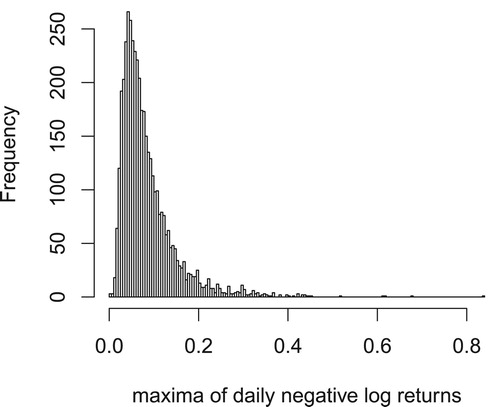
We find the 90th, 95th and 99th sample percentiles of $\{m_i{\}}_{i=1}^{4277}$, which are 0.1545, 0.2 and 0.3229, respectively. Here the daily maximal negative log returns have some time dependency. However, for the purpose of demonstration, we treat them as independent and fit the AMSD/AEVD and the GEV distribution to $\{m_i{\}}_{i=1}^{4277}$. Based on the fitted distributions, we generate random samples with the same size and find the proportions of the samples that exceed the three percentiles. The proportions are shown in Table 2.

Table 2. The proportions of the simulated samples generated from the fitted distributions that exceed the 90th, 95th, and 99th sample percentiles of the maximal daily negative log returns.

	90th		95th		99th
	AMSD	GEV	AMSD	GEV	AMSD	GEV
Proportion	0.0961	0.0954	0.0475	0.0521	0.0115	0.0140

Note: The numbers in bold font are the ones that are closer to the theoretical values, i.e., 0.1, 0.05, and 0.01, respectively.

Table 2 clearly reveals that the AMSD/AEVD performs better than the GEV alone. The modelling performance may be further improved if time series dependence is implemented in the model fitting, e.g., the AcF model proposed by Zhao et al. (2018) and Mao and Zhang (2018). We will leave this task as a future project.

6. Conclusions

This paper extends the classical extreme value theory to maxima of maxima of time series with mixture patterns depending on the sample size. It has been shown that the classical extreme value distributions are special cases of the accelerated max-stable (extreme value) distributions (AMSDs/AEVDs). Some basic probabilistic properties are presented in the paper. These properties can be used as the probability foundation of recently proposed statistical models for extreme observations. The AMSDs may shed the light of extreme value studies and inferences. Many of existing theories in classical extreme value literature can be renovated in a much more general setting. Many real applications, e.g., risk analysis and portfolio management, systemic risk, etc. can be reanalysed and better results can be expected. Under the newly introduced framework, many new statistical models can be introduced and explored.

Acknowledgments

The authors thank Editor Jun Shao and two referees for their valuable comments. The work by Cao was partially supported by NSF-DMS-1505367 and Wisconsin Alumni Research Foundation #MSN215758. The work by Zhang was partially supported by NSF-DMS-1505367 and NSF-DMS-2012298.

Disclosure statement

No potential conflict of interest was reported by the author(s).

Additional information

Funding

The work by Cao was partially supported by NSF-DMS-1505367 and Wisconsin Alumni Research Foundation #MSN215758. The work by Zhang was partially supported by National Science Foundation NSF-DMS-1505367 and NSF-DMS-2012298.

Notes on contributors

Wenzhi Cao

Wenzhi Cao is a PhD student from the statistics department at the University of Wisconsin-Madison. Cao received his bachelor degree in Mathematics from Nankai University. Cao's research areas include extreme value theory and machine learning.

Zhengjun Zhang

Zhengjun Zhang is Professor of Statistics at the University of Wisconsin. Zhang's main research areas of expertise are in financial time series and rare event modelling, virtual standard cryptocurrency, risk management, nonlinear dependence, asymmetric dependence, asymmetric and directed causal inference, gene-gene relationship in rare diseases.

Appendix

A.1. Proofs of Theorems and Propositions

A.1.1. Proof of Theorem 2.1

For Equation (4(4) $P\left(a_{2,n_2}\right(M_n-b_{2,n_2})\le x)\to H_1(ax+b)H_2\left(x\right).$(4) ), $\begin{array}{rl}& P\left(a_{2,n_2}\right(M_n-b_{2,n_2})\le x)\\ & =P(max(a_{2,n_2}(M_{1,n_1}-b_{2,n_2}),\\ & a_{2,n_2}(M_{2,n_2}-b_{2,n_2}))\le x)\\ & =P\left(a_{2,n_2}\right(M_{1,n_1}-b_{2,n_2})\\ & \le x,a_{2,n_2}(M_{2,n_2}-b_{2,n_2})\le x)\\ & =P\left(a_{1,n_1}(M_{1,n_1}-b_{1,n_1})\right.\\ & \le a_{1,n_1}\left(\frac{x}{a_{2,n_2}}+b_{2,n_2}-b_{1,n_1}\right),\\ & \left.a_{2,n_2}(M_{2,n_2}-b_{2,n_2})\le x\right)\\ & \to H_1(ax+b)H_2\left(x\right).\end{array}$For Equation (5(5) $P\left(a_{2,n_2}\right(M_n-b_{2,n_2})\le x)\to H_2\left(x\right).$(5) ), $\begin{array}{rl}& P\left(a_{2,n_2}\right(M_n-b_{2,n_2})\le x)\\ & =P(a_{1,n_1}(M_{1,n_1}-b_{1,n_1})\\ & \le a_{1,n_1}\left(\frac{x}{a_{2,n_2}}+b_{2,n_2}-b_{1,n_1}\right),\\ & a_{2,n_2}(M_{2,n_2}-b_{2,n_2})\le x)\\ & \to H_2\left(x\right).\end{array}$

A.1.2. Proof of Fact 2.2

The density of ${\mathrm{\Phi }}_{{\alpha }_1}{\mathrm{\Phi }}_{{\alpha }_2}$ is (A1) $f\left(x\right)=\left\{\begin{array}{ll}{\mathrm{e}}^{-x^{-{\alpha }_1}-x^{-{\alpha }_2}}({\alpha }_1{x}^{-{\alpha }_1-1}+{\alpha }_2{x}^{-{\alpha }_2-1}),& x\ge 0,\\ 0,& x<0.\end{array}\right.$(A1) Thus (A2) $\begin{array}{rl}{\mu }_k& ={\int }_0^{\mathrm{\infty }}{x}^{k}f\left(x\right)\mathrm{d}\left(x\right)\\ & ={\int }_0^{\mathrm{\infty }}{x}^k{\mathrm{e}}^{-x^{-{\alpha }_1}-x^{-{\alpha }_2}}({\alpha }_1{x}^{-{\alpha }_1-1}+{\alpha }_2{x}^{-{\alpha }_2-1})\mathrm{d}x.\end{array}$(A2) Dividing the integral into two parts, we get (A3) ${\mu }_k={\int }_0^1{x}^{k}f\left(x\right)\mathrm{d}x+{\int }_1^{\mathrm{\infty }}{x}^{k}f\left(x\right)\mathrm{d}x.$(A3) First, let us consider ${\int }_0^1{x}^{k}f\left(x\right)\mathrm{d}x$. Since $\underset{x\to 0}{lim}{x}^{k}f\left(x\right)=0$ and $x^{k}f\left(x\right)$ is continuous on $[0,1]$, it is bounded on $[0,1]$. This implies that (A4) ${\int }_0^1{x}^{k}f\left(x\right)\mathrm{d}x<\mathrm{\infty }.$(A4) Next, let us consider ${\int }_1^{\mathrm{\infty }}{x}^{k}f\left(x\right)\mathrm{d}x$. We have $\begin{array}{rl}& {\int }_1^{\mathrm{\infty }}{x}^{k}f\left(x\right)\mathrm{d}x\\ & ={\int }_1^{\mathrm{\infty }}{\mathrm{e}}^{-x^{-{\alpha }_1}-x^{-{\alpha }_2}}({\alpha }_1{x}^{k-{\alpha }_1-1}+{\alpha }_2{x}^{k-{\alpha }_2-1})\mathrm{d}x.\end{array}$Notice that (A5) $\underset{x\to \mathrm{\infty }}{lim}{\mathrm{e}}^{-x^{-{\alpha }_1}-x^{-{\alpha }_2}}=1.$(A5) Therefore ${\int }_1^{\mathrm{\infty }}{\mathrm{e}}^{-x^{-{\alpha }_1}-x^{-{\alpha }_2}}({\alpha }_1{x}^{k-{\alpha }_1-1}+{\alpha }_2{x}^{k-{\alpha }_2-1})\mathrm{d}x<\mathrm{\infty }$ only if $k<{\alpha }_1$ and $k<{\alpha }_2$, i.e., $k<min({\alpha }_1,{\alpha }_2)$.

A.1.3. Proof of Fact 2.3

We need to consider $\underset{x\to \mathrm{\infty }}{lim}\frac{1-{\mathrm{e}}^{-x^{-{\alpha }_1}}{\mathrm{e}}^{-x^{-{\alpha }_2}}}{1-{\mathrm{e}}^{-x^{-{\alpha }_1}}}$.

Since $x^{-{\alpha }_1}\to 0$ and $x^{-{\alpha }_2}\to 0$ as $x\to \mathrm{\infty }$, we have the Taylor expansions $\begin{array}{rl}{\mathrm{e}}^{-x^{-{\alpha }_1}}& =1-x^{-{\alpha }_1}+o\left(x^{-{\alpha }_1}\right),\\ {\mathrm{e}}^{-x^{-{\alpha }_1}-x^{-{\alpha }_2}}& =1-(x^{-{\alpha }_1}+x^{-{\alpha }_2})+o(x^{-{\alpha }_1}+x^{-{\alpha }_2}).\end{array}$Therefore (A6) $\begin{array}{rl}& \underset{x\to \mathrm{\infty }}{lim}\frac{1-{\mathrm{e}}^{-x^{-{\alpha }_1}}{\mathrm{e}}^{-x^{-{\alpha }_2}}}{1-{\mathrm{e}}^{-x^{-{\alpha }_1}}}\\ & =\underset{x\to \mathrm{\infty }}{lim}\frac{(x^{-{\alpha }_1}+x^{-{\alpha }_2})+o(x^{-{\alpha }_1}+x^{-{\alpha }_2})}{x^{-{\alpha }_1}+o\left(x^{-{\alpha }_1}\right)}\\ & =\underset{x\to \mathrm{\infty }}{lim}(1+x^{{\alpha }_1-{\alpha }_2})=1.\end{array}$(A6) This proves that ${\mathrm{\Phi }}_{{\alpha }_1}{\mathrm{\Phi }}_{{\alpha }_2}$ and ${\mathrm{\Phi }}_{{\alpha }_1}$ are tail-equivalent.

A.1.4. Proof of Fact 2.4

The density of $\mathrm{\Lambda }\left(x\right){\mathrm{\Phi }}_{\alpha }\left(x\right)$ is $f\left(x\right)=\left\{\begin{array}{ll}{\mathrm{e}}^{-{\mathrm{e}}^{-x}-x^{-\alpha }}({\mathrm{e}}^{-x}+\alpha x^{-\alpha -1}),& x\ge 0,\\ 0,& x<0.\end{array}\right.$Thus (A7) $\begin{array}{rl}{\mu }_k& ={\int }_0^{\mathrm{\infty }}{x}^{k}f\left(x\right)\mathrm{d}x\\ & ={\int }_0^{\mathrm{\infty }}{x}^k{\mathrm{e}}^{-{\mathrm{e}}^{-x}-x^{-\alpha }}({\mathrm{e}}^{-x}+\alpha x^{-\alpha -1})\mathrm{d}x.\end{array}$(A7) Dividing the above equation into two parts, we get (A8) ${\mu }_k={\int }_0^1{x}^{k}f\left(x\right)\mathrm{d}x+{\int }_1^{\mathrm{\infty }}{x}^{k}f\left(x\right)\mathrm{d}x.$(A8) For the first part, since $\underset{x\to 0}{lim}{x}^{k}f\left(x\right)=0$ and $x^{k}f\left(x\right)$ is continuous on $[0,1]$, it is bounded on $[0,1]$. Thus ${\int }_0^1{x}^{k}f\left(x\right)<\mathrm{\infty }$.

For the second part, (A9) ${\int }_1^{\mathrm{\infty }}{x}^{k}f\left(x\right)={\int }_1^{\mathrm{\infty }}{\mathrm{e}}^{-{\mathrm{e}}^{-x}-x^{-\alpha }}({\mathrm{e}}^{-x}{x}^k+\alpha x^{k-\alpha -1})\mathrm{d}x.$(A9) Since (A10) $\underset{x\to \mathrm{\infty }}{lim}{\mathrm{e}}^{-{\mathrm{e}}^{-x}-x^{-\alpha }}=1,\mathrm{a}\mathrm{n}\mathrm{d}{\int }_1^{\mathrm{\infty }}{\mathrm{e}}^{-x}{x}^k\mathrm{d}x<\mathrm{\infty }\mathrm{f}\mathrm{o}\mathrm{r}\mathrm{\forall }k,$(A10) we have ${\int }_1^{\mathrm{\infty }}{\mathrm{e}}^{-{\mathrm{e}}^{-x}-x^{-\alpha }}({\mathrm{e}}^{-x}{x}^k+\alpha x^{k-\alpha -1})\mathrm{d}x<\mathrm{\infty }$ if and only if $k<\alpha$.

A.1.5. Proof of Fact 2.5

We need to consider $\underset{x\to \mathrm{\infty }}{lim}\frac{1-{\mathrm{e}}^{-{\mathrm{e}}^{-x}}{\mathrm{e}}^{-x^{-\alpha }}}{1-{\mathrm{e}}^{-x^{-\alpha }}}$.

Since $\underset{x\to \mathrm{\infty }}{lim}{\mathrm{e}}^{-x}\to 0$ and $\underset{x\to \mathrm{\infty }}{lim}{x}^{-\alpha }\to 0$, we have the Taylor expansions $\begin{array}{rl}{\mathrm{e}}^{-{\mathrm{e}}^{-x}-x^{-\alpha }}& =1-{\mathrm{e}}^{-x}-x^{-\alpha }+o({\mathrm{e}}^{-x}+x^{-\alpha }),\\ {\mathrm{e}}^{-x^{-\alpha }}& =1-x^{-\alpha }+o\left(x^{-\alpha }\right).\end{array}$Thus (A11) $\begin{array}{rl}\underset{x\to \mathrm{\infty }}{lim}\frac{1-{\mathrm{e}}^{-{\mathrm{e}}^{-x}}{\mathrm{e}}^{-x^{-\alpha }}}{1-{\mathrm{e}}^{-x^{-\alpha }}}& =\underset{x\to \mathrm{\infty }}{lim}\frac{{\mathrm{e}}^{-x}+x^{-\alpha }+o({\mathrm{e}}^{-x}+x^{-\alpha })}{x^{-\alpha }+o\left(x^{-\alpha }\right)}\\ & =1.\end{array}$(A11) This implies that $\mathrm{\Lambda }\left(x\right){\mathrm{\Phi }}_{\alpha }\left(x\right)$ and ${\mathrm{\Phi }}_{\alpha }\left(x\right)$ are tail-equivalent.

A.1.6. Proof of Theorem 3.1

If (25(25) $\begin{array}{rl}& n_1(1-F_1(u_{1,n_1}\left)\right)+n_2(1-F_2(u_{2,n_2}\left)\right)\\ & \to \tau \mathrm{a}\mathrm{s}n\to \mathrm{\infty }.\end{array}$(25) ) holds, we must have $\begin{array}{rl}& 1-F_1\left(u_{1,n_1}\right)\to 0,\\ & 1-F_2\left(u_{2,n_2}\right)\to 0.\end{array}$Then (A12) $\begin{array}{rl}& n_1\log (1-(1-F_1\left(u_{1,n_1}\right)\left)\right)+n_2\log (1-(1-F_2\left(u_{2,n_2}\right)\left)\right)\\ & =-n_1(1-F_1(u_{1,n_1}\left)\right)(1+o(1\left)\right)\\ & -n_2(1-F_2(u_{2,n_2}\left)\right)(1+o(1\left)\right)\\ & \to -\tau ,\end{array}$(A12) which is equivalent to $\begin{array}{rl}& P(M_{1,n_1}\le u_{1,n_1},M_{2,n_2}\le u_{2,n_2})\\ & =(1-(1-F_1\left(u_{1,n_1}\right)\left){)}^{n_1}\right(1-(1-F_2(u_{2,n_2}\left)\right){)}^{n_2}\\ & =\exp \{n_1\log (1-(1-F_1\left(u_{1,n_1}\right)\left)\right)\\ & +n_2\log (1-(1-F_2\left(u_{2,n_2}\right)\left)\right)\}\\ & \to {\mathrm{e}}^{-\tau }.\end{array}$Conversely, if (26(26) $P(M_{1,n_1}\le u_{1,n_1},M_{2,n_2}\le u_{2,n_2})\to {\mathrm{e}}^{-\tau }\mathrm{a}\mathrm{s}n\to \mathrm{\infty }.$(26) ) holds, which is equivalent to (A13) $\begin{array}{rl}& n_1\log (1-(1-F_1\left(u_{1,n_1}\right)\left)\right)\\ & +n_2\log (1-(1-F_2\left(u_{2,n_2}\right)\left)\right)\to -\tau ,\end{array}$(A13) we must have $1-F_1\left(u_{1,n_1}\right)\to 0$ and $1-F_2\left(u_{2,n_2}\right)\to 0$. Otherwise, suppose $1-F_1\left(u_{1,n_1}\right)\nrightarrow 0$, then there is a sequence of indexes $m_1,m_2,\dots$ and $ϵ>0$ such that $1-F_1\left(u_{1,m_k}\right)>ϵ$ for $\mathrm{\forall }k$. This means that $\begin{array}{rl}& n_1\log (1-(1-F_1\left(u_{1,m_i}\right)\left)\right)+n_2\log (1-(1-F_2\left(u_{2,n-m_i}\right)\left)\right)\\ & <n_1\log (1-(1-F_1\left(u_{1,m_i}\right)\left)\right)\\ & <n_1\log (1-ϵ)\to -\mathrm{\infty },\end{array}$which is contradictory to (A13(A13) $\begin{array}{rl}& n_1\log (1-(1-F_1\left(u_{1,n_1}\right)\left)\right)\\ & +n_2\log (1-(1-F_2\left(u_{2,n_2}\right)\left)\right)\to -\tau ,\end{array}$(A13) ). We have (A14) $\begin{array}{rl}& n_1\left[\right(1-F_1\left(u_{1,n_1}\right))+o(1-F_1\left(u_{1,n_1}\right)\left)\right]\\ & +n_2\left[\right(1-F_2\left(u_{2,n_2}\right))+o(1-F_2\left(u_{2,n_2}\right)\left)\right]\to \tau \end{array}$(A14) and Equation (25(25) $\begin{array}{rl}& n_1(1-F_1(u_{1,n_1}\left)\right)+n_2(1-F_2(u_{2,n_2}\left)\right)\\ & \to \tau \mathrm{a}\mathrm{s}n\to \mathrm{\infty }.\end{array}$(25) ) holds.

A.1.7. Proof of Corollary 3.1

Since (A15) $n_1(1-F_1(u_{1,n_1}\left)\right)+n_2(1-F_2(u_{2,n_2}\left)\right)\to {\tau }_1+{\tau }_2,$(A15) (30(30) $P(M_{1,n_1}\le u_{1,n},M_{2,n_2}\le u_{2,n})\to {\mathrm{e}}^{-{\tau }_1-{\tau }_2}.$(30) ) is a direct result of Theorem 3.1.

If $\frac{n_2(1-F_2(u_{1,n_1}\left)\right)}{n_1(1-F_1(u_{1,n_1}\left)\right)}\to t$, then $n_2(1-F_2(u_{1,n_1}\left)\right)\to t{\tau }_1$, where $0\le t{\tau }_1<\mathrm{\infty }$. Therefore, $\begin{array}{rl}P(M_n\le u_{1,n_1})& =P(M_{1,n_1}\le u_{1,n_1})P(M_{2,n_2}\le u_{1,n_1})\\ & \to {\mathrm{e}}^{-{\tau }_1(1+t)}.\end{array}$

A.1.8. Proof of Theorem 3.2

Since $P(M_{i,n_i}\le u_{i,n_i})=(1-{\tau }_{i,n_i}/n_i{)}^{n_i}$ and $0\le {\tau }_{i,n_i}=n_1(1-F_i(u_{i,n_i}\left)\right)\le n$, the result follows from Lemma A.2.

A.1.9. Proof of Theorem 4.1

For fixed k, write $n^{\prime }=\left[n/k\right]$, suppose that there are $n_1^{\prime }$ members from $F_1$ and $n_2^{\prime }$ members from $F_2$ among $\{X_1,\dots ,X_{n^{\prime }}\},$ $n^{\prime }=n_1^{\prime }+n_2^{\prime }$. If (47(47) $n_1(1-F_1(u_{1,n_1}\left)\right)+n_2(1-F_2(u_{2,n_2}\left)\right)\to \tau .$(47) ) holds, by assumption we have $n_1^{\prime }\sim p{n}^{\prime }\sim \frac{n_1}{k}$ and $n_2^{\prime }\sim (1-p)n^{\prime }\sim \frac{n_2}{k},$ thus (A16) $n_1^{\prime }(1-F_1(u_{1,n_1}\left)\right)+n_2^{\prime }(1-F_2(u_{2,n_2}\left)\right)\to \frac{\tau }{k}.$(A16) Since $\begin{array}{rl}& P\left(\right\{M_{1,n_1^{\prime }}\le u_{1,n_1},M_{2,n_2^{\prime }}\le u_{2,n_2}\left\}\right)\\ & =1-P\left(\right\{M_{1,n_1^{\prime }}>u_{1,n_1}\}\cup \{M_{2,n_2^{\prime }}>u_{2,n_2}\left\}\right)\\ & =1-P\left(\left(\bigcup _{i=1}^{n_1^{\prime }}\{X_{1,i}>u_{1,n_1}\}\right)\cup \left(\bigcup _{j=1}^{n_2^{\prime }}\{X_{2,j}>u_{2,n_2}\}\right)\right),\end{array}$we have (A17) $\begin{array}{rl}& 1-n_1^{\prime }(1-F_1(u_{1,n_1}\left)\right)-n_2^{\prime }(1-F_2(u_{2,n_2}\left)\right)\\ & \le P(M_{1,n_1^{\prime }}\le u_{1,n_1},M_{2,n_2^{\prime }}\le u_{2,n_2})\\ & \le 1-n_1^{\prime }(1-F_1(u_{1,n_1}\left)\right)-n_2^{\prime }(1-F_2(u_{2,n_2}\left)\right)+S_n,\end{array}$(A17) where $S_n=\sum _{1\le i<j\le n^{\prime }}P(X_i>u_n^{\left(i\right)},X_j>u_n^{\left(j\right)})$.

Condition $D^{\prime }\left({\mathbf{u}}_n\right)$ implies that $\underset{n\to \mathrm{\infty }}{lim sup}{S}_n=o\left(\frac{1}{k}\right)$ as $k\to \mathrm{\infty }$. By (A16(A16) $n_1^{\prime }(1-F_1(u_{1,n_1}\left)\right)+n_2^{\prime }(1-F_2(u_{2,n_2}\left)\right)\to \frac{\tau }{k}.$(A16) ) and (A17(A17) $\begin{array}{rl}& 1-n_1^{\prime }(1-F_1(u_{1,n_1}\left)\right)-n_2^{\prime }(1-F_2(u_{2,n_2}\left)\right)\\ & \le P(M_{1,n_1^{\prime }}\le u_{1,n_1},M_{2,n_2^{\prime }}\le u_{2,n_2})\\ & \le 1-n_1^{\prime }(1-F_1(u_{1,n_1}\left)\right)-n_2^{\prime }(1-F_2(u_{2,n_2}\left)\right)+S_n,\end{array}$(A17) ), we have $\begin{array}{rl}1-\frac{\tau }{k}& \le \underset{n\to \mathrm{\infty }}{lim inf}P(M_{1,n_1^{\prime }}\le u_{1,n_1},M_{2,n_2^{\prime }}\le u_{2,n_2})\\ & \le \underset{n\to \mathrm{\infty }}{lim sup}P(M_{1,n_1^{\prime }}\le u_{1,n_1},M_{2,n_2^{\prime }}\le u_{2,n_2})\\ & \le 1-\frac{\tau }{k}+o\left(\frac{1}{k}\right).\end{array}$Since $D\left({\mathbf{u}}_n\right)$ implies $D\left(u_{1,n_1}\right)$ and $D\left(u_{2,n_2}\right)$, Lemma A.3 holds for each subsequence. We have $\begin{array}{rl}{\left(1-\frac{\tau }{k}\right)}^k& \le \underset{n\to \mathrm{\infty }}{lim inf}P(M_{1,n_1}\le u_{1,n_1},M_{2,n_2}\le u_{2,n_2})\\ & \le \underset{n\to \mathrm{\infty }}{lim sup}P(M_{1,n_1}\le u_{1,n_1},M_{2,n_2}\le u_{2,n_2})\\ & \le {\left(1-\frac{\tau }{k}+o\left(\frac{1}{k}\right)\right)}^k.\end{array}$Letting $k\to \mathrm{\infty },$ we have $\underset{n\to \mathrm{\infty }}{lim}P(M_{1,n_1}\le u_{1,n_1},M_{2,n_2}\le u_{2,n_2})\to {\mathrm{e}}^{-\tau }$.

Conversely, if (46(46) $P(M_{1,n_1}\le u_{1,n_1},M_{2,n_2}\le u_{2,n_2})\to {\mathrm{e}}^{-\tau }$(46) ) holds, (A18) $\begin{array}{rl}& 1-P(M_{1,n_1^{\prime }}\le u_{1,n_1},M_{2,n_2^{\prime }}\le u_{2,n_2})\\ & \le n_1^{\prime }(1-F_1(u_{1,n_1}\left)\right)+n_2^{\prime }(1-F_2(u_{2,n_2}\left)\right)\\ & \le 1-P(M_{1,n_1^{\prime }}\le u_{1,n_1},M_{2,n_2^{\prime }}\le u_{2,n_2})+S_n.\end{array}$(A18) Since $P(M_{1,n_1}\le u_{1,n_1},M_{2,n_2}\le u_{2,n_2})\to {\mathrm{e}}^{-\tau },$ we have $P(M_{1,n_1^{\prime }}\le u_{1,n_1},M_{2,n_2^{\prime }}\le u_{2,n_2})\to {\mathrm{e}}^{-\tau /k}$. By letting $n\to \mathrm{\infty }$ in (A18(A18) $\begin{array}{rl}& 1-P(M_{1,n_1^{\prime }}\le u_{1,n_1},M_{2,n_2^{\prime }}\le u_{2,n_2})\\ & \le n_1^{\prime }(1-F_1(u_{1,n_1}\left)\right)+n_2^{\prime }(1-F_2(u_{2,n_2}\left)\right)\\ & \le 1-P(M_{1,n_1^{\prime }}\le u_{1,n_1},M_{2,n_2^{\prime }}\le u_{2,n_2})+S_n.\end{array}$(A18) ), $\begin{array}{rl}& 1-{\mathrm{e}}^{-\tau /k}\\ & \le \frac{1}{k}\underset{n\to \mathrm{\infty }}{lim inf}{n}_1(1-F_1(u_{1,n_1}\left)\right)+n_2(1-F_2(u_{2,n_2}\left)\right)\\ & \le \frac{1}{k}\underset{n\to \mathrm{\infty }}{lim sup}{n}_1(1-F_1(u_{1,n_1}\left)\right)+n_2(1-F_2(u_{2,n_2}\left)\right)\\ & \le 1-{\mathrm{e}}^{-\tau /k}+o\left(\frac{1}{k}\right)\end{array}$from which (multiplying k on all sides and let $k\to \mathrm{\infty }$) we have $n_1(1-F_1(u_{1,n_1}\left)\right)+n_2(1-F_2(u_{2,n_2}\left)\right)\to \tau$.

A.1.10. Proof of Corollary 4.1

Suppose $n_1(1-F_1(u_{1,n_1}\left)\right)+n_2(1-F_2(u_{2,n_2}\left)\right)\to \mathrm{\infty },$ by $u_{1,n_1}<v_{1,n_1}$ and $u_{2,n_2}<v_{2,n_2}$, we have $\begin{array}{rl}P(M_{1,n_1}& \le u_{1,n_1},M_{2,n_2}\le u_{2,n_2})\\ & \le P(M_{1,n_1}\le v_{1,n_1},M_{2,n_2}\le v_{2,n_2}).\end{array}$By Theorem 4.1, $P(M_{1,n_1}\le v_{1,n_1},M_{2,n_2}\le v_{2,n_2})\to {\mathrm{e}}^{-\tau }$. Then $\underset{n\to \mathrm{\infty }}{lim sup}P(M_{1,n_1}\le u_{1,n_1},M_{2,n_2}\le u_{2,n_2})\le {\mathrm{e}}^{-\tau }.$By letting $\tau \to \mathrm{\infty }$, we have $\underset{n\to \mathrm{\infty }}{lim}P(M_{1,n_1}\le u_{1,n_1},M_{2,n_2}\le u_{2,n_2})=0.$Conversely, we still have $\begin{array}{rl}& n_1(1-F_1(u_{1,n_1}\left)\right)+n_2(1-F_2(u_{2,n_2}\left)\right)\\ & \ge n_1(1-F_1(v_{1,n_1})+n_2(1-F_2\left(v_{2,n_2}\right))\to \tau .\end{array}$Since the above inequality holds for arbitrary large $\tau >0,$ we must have $n_1(1-F_1(u_{1,n_1}\left)\right)+n_2(1-F_2(u_{2,n_2}\left)\right)\to \mathrm{\infty }$.

A.1.11. Proof of Theorem 4.2

For $\theta >0$, the condition $P({\hat{M}}_{1,n_1}\le u_{1,n_1},{\hat{M}}_{2,n_2}\le u_{2,n_2})\to \theta$ may be rewritten as $P({\hat{M}}_{1,n_1}\le u_{1,n_1},{\hat{M}}_{2,n_2}\le u_{2,n_2})\to {\mathrm{e}}^{-\tau }$ with $\tau =-\log \theta$, this holds if and only if $n_1(1-F_1(u_{1,n_1}\left)\right)+n_2(1-F_2(u_{2,n_2}\left)\right)\to \tau$. The same is true for $P(M_{1,n_1}\le u_{1,n_1},M_{2,n_2}\le u_{2,n_2})$ by condition $D\left({\mathbf{u}}_n\right)$ and $D^{\prime }\left({\mathbf{u}}_n\right)$. When $\theta =0$, the result follows from Corollary 4.1.

A.1.12. Proof of Theorem 4.3

If $G\left(x\right)>0$, the equivalence follows from Theorem 4.2, with $\theta =G\left(x\right)$.

If $G\left(x\right)=0$, the continuity of G shows that, if $0<\tau <\mathrm{\infty }$,there exists $x_0$ such that $G\left(x_0\right)={\mathrm{e}}^{-\tau }$. $D\left(v_{i,n_i}\right)$ and $D^{\prime }\left(v_{i,n_i}\right)$ hold for $v_{1,n_1}=x_0/a_{1,n_1}+b_{1,n_1},v_{2,n_2}=x_0/a_{2,n_2}+b_{2,n_2}$ and $P(M_{1,n_1}\le v_{1,n_1},M_{2,n_2}\le v_{2,n_2})\to {\mathrm{e}}^{-\tau }$ or $P({\hat{M}}_{1,n_1}\le v_{1,n_1},{\hat{M}}_{2,n_2}\le v_{2,n_2})\to {\mathrm{e}}^{-\tau }$ depending on the assumption made, so that $n_1(1-F_1(v_{1,n_1}\left)\right)+n_2(1-F_2(v_{2,n_2}\left)\right)\to \tau$. If (49(49) $\begin{array}{rl}& P\left(a_{1,n_1}\right({\hat{M}}_{1,n_1}-b_{1,n_1})\\ & \le x,a_{2,n_2}({\hat{M}}_{2,n_2}-b_{2,n_2})\le x)\to G(x)\end{array}$(49) ) holds, then we have $n_1(1-F_1(u_{1,n_1}\left)\right)+n_2(1-F_2(u_{2,n_2}\left)\right)\to \mathrm{\infty },$ thus $u_{1,n_1}<v_{1,n_1}$ and $u_{2,n_2}<v_{2,n_2}$ (since one of the inequalities must hold and also implies another). By Theorem 4.2, (48(48) $\begin{array}{rl}& P\left(a_{1,n_1}\right(M_{1,n_1}-b_{1,n_1})\\ & \le x,a_{2,n_2}(M_{2,n_2}-b_{2,n_2})\le x)\to G(x)\end{array}$(48) ) holds. The converse direction can be proved similarly.

A.2. Lemmas

Lemma A.1

Khintchine, Theorem 1.2.3 in Leadbetter et al. (2012)

Let $\left\{F_n\right\}$ be a sequence of cdf's and H a nondegenerate cdf. Let $a_n>0$ and $b_n$ be constants such that (A19) $F_n(a_{n}x+b_n)\stackrel{w}{\to }H\left(x\right).$(A19) Then for some nondegenerate cdf $H_{\ast }$ and constants ${\alpha }_n>0$, ${\text{β}}_n$, (A20) $F_n({\alpha }_{n}x+{\text{β}}_n)\stackrel{w}{\to }{H}_{\ast }\left(x\right)$(A20) if and only if (A21) $a_n^{-1}{\alpha }_n\to a\mathrm{a}\mathrm{n}\mathrm{d}{a}_n^{-1}({\text{β}}_n-b_n)\to b$(A21) for some a>0 and b, and then (A22) $H_{\ast }\left(x\right)=H(ax+b).$(A22)

Lemma A.2

Lemma 2.4.1 in Leadbetter et al. (2012)

1. If $0\le x\le n$ then (A23) $\begin{array}{rl}0\le {\mathrm{e}}^{-x}-{\left(1-\frac{x}{n}\right)}^n& \le \frac{x^2{\mathrm{e}}^{-x}}{2}\cdot \frac{1}{n-1}\\ & \le 2{\mathrm{e}}^{-2}\cdot \frac{1}{n-1}\\ & \le 0.3\cdot \frac{1}{n-1}\mathrm{f}\mathrm{o}\mathrm{r}n=1,2,\dots ,\end{array}$(A23) and further (A24) $\begin{array}{rl}& {\mathrm{e}}^{-x}-{\left(1-\frac{x}{n}\right)}^n\\ & =\frac{x^2{\mathrm{e}}^{-x}}{2}\frac{1}{n}\left(1+O\left(\frac{1}{n}\right)\right)\mathrm{a}\mathrm{s}n\to \mathrm{\infty },\end{array}$(A24) uniformly for x in bounded intervals.

2. If $x-y\le \log 2$ then (A25) ${\mathrm{e}}^{-y}-{\mathrm{e}}^{-x}={\mathrm{e}}^{-x}\left\{\right(x-y)+\theta (x-y{)}^2\},$(A25) with $0<\theta <1$.

Lemma A.3

Lemma 3.3.2 in Leadbetter et al. (2012)

If $D\left(u_n\right)$ holds, for a fixed integer k, we have (A26) $P(M_n\le u_n)-P^k(M_{\left[n/k\right]}\le u_n)\to 0\mathrm{a}\mathrm{s}n\to \mathrm{\infty }.$(A26)

References

- Beirlant, J., Goegebeur, Y., Segers, J., & Teugels, J. (2004). Statistics of extremes: Theory and applications. Wiley Series in Probability and Statistics. Wiley.
- Bücher, A., & Segers, J. (2017). On the maximum likelihood estimator for the generalized extreme-value distribution. Extremes, 20(4), 839–872. https://doi.org/https://doi.org/10.1007/s10687-017-0292-6
- Castillo, E., Hadi, A. S., Balakrishnan, N., & Sarabia, J. M. (2005). Extreme value and related models with applications in engineering and science. Wiley Series in Probability and Statistics. Wiley.
- Chavez-Demoulin, V., Embrechts, P., & Hofert, M. (2016). An extreme value approach for modeling operational risk losses depending on covariates. Journal of Risk and Insurance, 83(3), 735–776. https://doi.org/https://doi.org/10.1111/jori.v83.3
- Coles, S. (2001). An introduction to statistical modeling of extreme values. Springer.
- Daouia, A., Girard, S., & Stupfler, G. (2018). Estimation of tail risk based on extreme expectiles. Journal of the Royal Statistical Society: Series B (Statistical Methodology), 80(2), 263–292. https://doi.org/https://doi.org/10.1111/rssb.12254
- de Haan, L. (1993). Extreme value statistics. In J. Galambos, J. Lechner, & E. Simiu (Eds.), Extreme value theory and applications (pp. 93–122). Kluwer Academic Publisher.
- de Haan, L., & Ferreira, A. (2006). Extreme value theory: An introduction. Springer Verlag.
- Dey, D. K., & Yan, J. (2016). Extreme value modeling and risk analysis: Methods and applications. Chapman & Hall/CRC.
- Embrechts, P., Resnick, S. I., & Samorodnitsky, G. (1999). Extreme value theory as a risk management tool. North American Actuarial Journal, 3(2), 30–41. https://doi.org/https://doi.org/10.1080/10920277.1999.10595797
- Finkenstädt, B., & Rootzén, H. E. (2004). Extreme values in finance, telecommunications, and the environment. Chapman & Hall/CRC.
- Galambos, J. (1978). The asymptotic theory of extreme order statistics. Technical Report.
- Heffernan, J. E., Tawn, J. A., & Zhang, Z. (2007). Asymptotically (in)dependent multivariate maxima of moving maxima processes. Extremes, 10(1–2), 57–82. https://doi.org/https://doi.org/10.1007/s10687-007-0035-1
- Idowu, T., & Zhang, Z. (2017). An extended sparse max-linear moving model with application to high-frequency financial data. Statistical Theory and Related Fields, 1(1), 92–111. https://doi.org/https://doi.org/10.1080/24754269.2017.1346852
- Leadbetter, M. R., Lindgren, G., & Rootzén, H. (2012). Extremes and related properties of random sequences and processes. Springer Science & Business Media.
- Loynes, R. M. (1965). Extreme values in uniformly mixing stationary stochastic processes. The Annals of Mathematical Statistics, 36(3), 993–999. https://doi.org/https://doi.org/10.1214/aoms/1177700071
- Malinowski, A., Schlather, M., & Zhang, Z. (2015). Marked point process adjusted tail dependence analysis for high-frequency financial data. Statistics and Its Interface, 8(1), 109–122. https://doi.org/https://doi.org/10.4310/SII.2015.v8.n1.a10
- Mao, G., & Zhang, Z. (2018). Stochastic tail index model for high frequency financial data with Bayesian analysis. Journal of Econometrics, 205(2), 470–487. https://doi.org/https://doi.org/10.1016/j.jeconom.2018.03.019
- McNeil, A. J., & Frey, R. (2000). Estimation of tail-related risk measures for heteroscedastic financial time series: An extreme value approach. Journal of Empirical Finance, 7(3–4), 271–300. https://doi.org/https://doi.org/10.1016/S0927-5398(00)00012-8
- Mikosch, T., Embrechts, P., & Klüppelberg, C. (1997). Modelling extremal events for insurance and finance. Springer Verlag.
- Naveau, P., Zhang, Z., & Zhu, B. (2011). An extension of max autoregressive models. Statistics and Its Interface, 4(2), 253–266. https://doi.org/https://doi.org/10.4310/SII.2011.v4.n2.a19
- Resnick, S. I. (2013). Extreme values, regular variation and point processes. Springer.
- Rocco, M. (2014). Extreme value theory in finance: A survey. Journal of Economic Surveys, 28(1), 82–108. https://doi.org/https://doi.org/10.1111/joes.2014.28.issue-1
- Rosenblatt, M. (1956). A central limit theorem and a strong mixing condition. Proceedings of the National Academy of Sciences USA, 42(1), 43–47. https://doi.org/https://doi.org/10.1073/pnas.42.1.43
- Salvadori, G., De Michele, C., Kottegoda, N. T., & Rosso, R. (2007). Extremes in nature: An approach using copulas. Springer(Complexity).
- Smith, R. L. (1985). Maximum likelihood estimation in a class of nonregular cases. Biometrika, 72(1), 67–90. https://doi.org/https://doi.org/10.1093/biomet/72.1.67
- Tang, R., Shao, J., & Zhang, Z. (2013). Sparse moving maxima models for tail dependence in multivariate financial time series. Journal of Statistical Planning and Inference, 143(5), 882–895. https://doi.org/https://doi.org/10.1016/j.jspi.2012.11.008
- Tsay, R. S. (2005). Analysis of financial time series (Vol. 543). John Wiley & Sons.
- Watson, G. S. (1954). Extreme values in samples from m-dependent stationary stochastic processes. The Annals of Mathematical Statistics, 25(4), 798–800. https://doi.org/https://doi.org/10.1214/aoms/1177728670
- Zhang, Z., & Smith, R. L. (2010). On the estimation and application of max-stable processes. Journal of Statistical Planning and Inference, 140(5), 1135–1153. https://doi.org/https://doi.org/10.1016/j.jspi.2009.10.014
- Zhang, Z., & Zhu, B. (2016). Copula structured m4 processes with application to high-frequency financial data. Journal of Econometrics, 194(2), 231–241. https://doi.org/https://doi.org/10.1016/j.jeconom.2016.05.004
- Zhao, Z., & Zhang, Z. (2018). Semi-parametric dynamic max-copula model for multivariate time series. Journal of the Royal Statistical Society: Series B (Statistical Methodology), 80(2), 409–432. https://doi.org/https://doi.org/10.1111/rssb.12256
- Zhao, Z., Zhang, Z., & Chen, R. (2018). Modeling maxima with autoregressive conditional Fréchet model. Journal of Econometrics, 207(2), 325–351. https://doi.org/https://doi.org/10.1016/j.jeconom.2018.07.004