Research on three-step accelerated gradient algorithm in deep learning

Abstract

Gradient descent (GD) algorithm is the widely used optimisation method in training machine learning and deep learning models. In this paper, based on GD, Polyak's momentum (PM), and Nesterov accelerated gradient (NAG), we give the convergence of the algorithms from an initial value to the optimal value of an objective function in simple quadratic form. Based on the convergence property of the quadratic function, two sister sequences of NAG's iteration and parallel tangent methods in neural networks, the three-step accelerated gradient (TAG) algorithm is proposed, which has three sequences other than two sister sequences. To illustrate the performance of this algorithm, we compare the proposed algorithm with the three other algorithms in quadratic function, high-dimensional quadratic functions, and nonquadratic function. Then we consider to combine the TAG algorithm to the backpropagation algorithm and the stochastic gradient descent algorithm in deep learning. For conveniently facilitate the proposed algorithms, we rewite the R package ‘neuralnet’ and extend it to ‘supneuralnet’. All kinds of deep learning algorithms in this paper are included in ‘supneuralnet’ package. Finally, we show our algorithms are superior to other algorithms in four case studies.

Keywords:

• Accelerated algorithm
• backpropagation
• deep learning
• learning rate
• momentum
• stochastic gradient descent

1. Introduction

In recent years, the scale of the industrial application system has expanded rapidly and industrial application data generated with the exponential growth due to the recent advance in computer and information technology. Big Data brings allround thinking revolution, industrial revolution, and management revolution because Big Data has vast amounts of data status and cloud service-level data processing ability, and Big Data has Volume, Velocity, Variety, and Veracity (also called 4V) characteristics. The data of enterprises has reached hundreds of TBs or hundreds of PBs which has been far beyond the processing capacity of traditional computing technology and information system. Therefore, to study effective Big Data processing technology, methods, and measurements have become urgent requirements in our daily lives.

Viktor Mayer-Schonberger, who is known as ‘the Prophet of Big Data Era’, lists a large number of detailed cases of Big Data applications in his book ‘Big Data: A Revolution That Will Transform How We Live, Work, and Think (Schonberger & Cukier, 2013)’. He analysed and predicted the development and trends of Big Data, and put forward many important ideas and development strategies. He said Big Data opens up a great transformation stage and stated that Big Data will bring great changes. It will change our lives, work and way of thinking, change our business mode, and change our economics, politics, technologies, societies, and so on.

‘The Outline of Promoting Development of Big Data’ was published by the State Council of China in September 2015. The Prime Minister of China Keqiang Li said we should deploy Big Data program systematically. The ‘Outline’ showed us how to promote Big Data development and application, to create accurate control and the collaborative new social governance mode in the next 5 to 10 years. Big Data can establish a new mechanism of economic operation, which is safe, efficient, and operates steadily. Big Data also can construct a new system about public services which is people oriented and benefits all, can open the new pattern of innovation driven which makes more people to have the sense of entrepreneurship and innovation, can cultivate the new environment of industry development which is intelligent, smart, and prosperous.

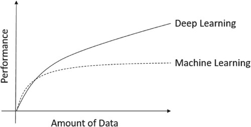
Machine learning and deep learning are very important big data processing technologies. Especially for deep learning, which is very popular in industry and academia in recent years. An important reason is that Google has developed AlphaGo. AlphaGo is the first artificial intelligence system that defeated professional Go players, and the first one defeated the Go world champion. It was developed by a team led by Demis Hassabis from Google's DeepMind company, and its main working principle is ‘deep learning’. AlphaGo uses many new technologies, such as neural networks (Flach, 2012), deep learning (Lisa, 2015), Monte Carlo tree search (Bishop, 2006; Murphy, 2012) etc., which has made a substantial power in training data and prediction. The performance of deep learning is shown in Figure 1. It can be seen from the figure that as the amount of data increases, compared with machine learning, the performance of deep learning becomes better and better.

Figure 1. The performance comparison of deep learning and machine learning.

Feedforward neural networks are the most basic type of artificial neural networks. The connections between neurons in the network do not form a cycle. Feedforward neural networks are the first type of artificial neural networks. The reason why they are called feedforward is because the information in these networks is only forwarded, do not have loops. The information first through the input nodes, then through the hidden nodes (if present), and finally through the output nodes (Nielsen, 2019). In industry and academia, a neural network is called deep learning which has at least one hidden layer.

Gradient descent (GD) algorithm is an optimisation algorithm used to minimise some function by iteratively moving in the direction of steepest descent as defined by the negative of the gradient. In artificial neural networks, backpropagation is a specific implementation method of the gradient descent algorithm. The name of the backpropogation algorithm originates from the process of calculating the gradient of the neural network, which is actually calculated backward (Rumelhart & McClelland, 1986). It is the most extensively used algorithm for training multilayer feedforward neural networks. Given an artificial neural network and an error function, then backpropagation is mainly to calculate the gradient of the error function with respect to the weights of the neural network. However, throughout the current books and literatures (Chen, 2016; Gordon, 2018; Le, 2015; Magoulas et al., 1997; Moreira & Fiesler, 1995), the mathematical representations of the backpropagation algorithm are different. This paper will present it in the subsequent sections with mathematical formulas.

The actual proceeding is that the gradient of the last layer of weights are calculated first, and the gradient of the first layer of weights are calculated last. When calculating the gradient of the previous layer, the partial derivatives which have been calculated in the current layer can be reused. This technique can be clearly seen when introducing deep learning neural networks in subsequent sections, and it is also very important in programming. It can not only save the time of program running, but also save the memory used by this program. Therefore, the backwards flow of the error information makes the gradient of the weights of each layer can be calculated efficiently, instead of using a very naive method to calculate the gradient separately.

The popularity of backpropagation has been reappeared in recent years, the main reason is that deep neural networks have obvious advantages in image recognition and speech recognition. Backpropagation is an iterative gradient descent algorithm. With the cooperation of Graphics Processing Unit (GPU), its performance has been greatly improved. However, from Churchland and Sejnowski (2016), Rumelhart et al. (1986), it is well known that such a learning scheme can be very slow. So various methods have been created to improve the conventional backpropagation efficiency. Momentum algorithms, first proposed by Polyak (1964), are well known techniques to accelerate deterministic smooth convex optimisation. Recently, Lan (2009, 2012) and Deng et al. (2018) have incorporated these techniques into optimisation.

Intuitively, the reason for using the momentum is that the GD algorithm is very slow when the error function surface is a very long and narrow valley. In this case, the gradient direction of the GD algorithm is almost perpendicular to the long axis of the valley. This causes the iteration to oscillate back and forth in the short axis while moving very slowly in the long axis of the valley. Qian (1999) pointed out that the role of momentum is to correct the gradient direction from the short axis to the long axis of the valley.

Besides, other methods have also been proposed for improving the speed of convergence of GD algorithm. The conjugate gradient algorithm has been shown to be superior to the GD algorithm in most applications, see Press et al. (1992). But this algorithm is less biologically plausible and harder to implement on hardware. Qian (1999) indicated the momentum algorithm appears to be dominant in the connectionist learning literature. The Polyak momentum (PM) algorithm does not converge in relatively simple convex optimisation problems. Nesterov (1983, 2004) made further improvements to the PM algorithm, which was later called the Nesterov accelerated gradient (NAG) algorithm. Nesterov's idea is that the improved algorithm should have the same acceleration effect as the PM algorithm, but it must converge for general convex functions optimisation problems. Finally, Nesterov proposed a pair of sister sequences which have correction effect on the direction of the iteration points of the algorithm.

In the global optimisation problems, Shah et al. (1964) and Petalas and Vrahatis (2004) used the parallel tangent method to improve the GD algorithm and speed up its convergence. The main idea of the parallel tangent method is that during the iteration, it use the parallel tangent direction occasionally instead of the gradient descent direction $-\mathrm{\nabla }f\left(x_i\right)$. Based on NAG algorithm, parallel tangent method, and some properties of optimal gradient descent with quadratic function, we propose a three-step accelerated gradient (TAG) algorithm, which has three sequences.

This paper mainly researches the TAG algorithm and applies it to deep learning, and compares it with the traditional GD algorithm, PM algorithm, and NAG algorithm. The rest of the paper proceeds as follows. Section 2 introduces GD, PM and NAG algorithms, then the TAG algorithm is developed, implements them to the quadratic function. Then the paper conducts experiments to high-dimensional functions, which help us to understand TAG with the fastest convergence among these four algorithms. Section 3 introduces deep learning and backpropagation algorithm. Then the TAG algorithm is added to the backpropagation algorithm. Since the R language package ‘neuralnet’ only contains the GD algorithm, we write a new package ‘supneuralnet’, which extend the PM algorithm, NAG algorithm, and TAG algorithm to the ‘neuralnet’ package. We also add the stochastic gradient descent (SGD) algorithm to the package, which is convenient to implement these algorithms. Section 4 applies the four algorithms to the iris and spiral data sets in the deep learning framework, to compare their classification effects and convergence speed. The proposed algorithm performs best. Section 5 combines the SGD algorithm with the four algorithms mentioned in Section 2, and applies them to the iris and spiral data sets under the deep learning framework to compare their classification effects and convergence speed. The proposed algorithm also performs best. Finally we draw conclusions in Section 6.

2. Three-step accelerated gradient algorithm

2.1. Gradient descent algorithm

From Yin (2015), we have the main iteration steps of GD algorithm are (1) $x_i=x_{i-1}-\alpha \mathrm{\nabla }f\left(x_{i-1}\right),$(1) for $i=2,3,\dots$. Here $f\left(x\right):{\mathbb{R}}^n\to \mathbb{R}$ is a differentiable function, its gradient is $\mathrm{\nabla }f\left(x\right)$, and α is step size.

Assume that A is symmetric and positive definite ($x^{\mathrm{T}}Ax>0$ for any $x\ne 0$). 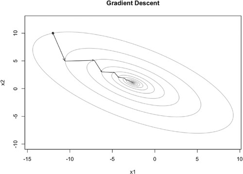Consider the quadratic function (2) $f\left(x\right)=\frac{1}{2}{x}^{\mathrm{T}}Ax+b^{\mathrm{T}}x+c,$(2) with (3) $\mathrm{\nabla }f\left(x\right)=Ax+b.$(3) Let $A=\left[\begin{array}{cc}6& 5\\ 5& 10\end{array}\right],b=\left(\begin{array}{c}10\\ 2\end{array}\right),x_1=\left(\begin{array}{c}-12\\ 10\end{array}\right).$Then we can show GD iteration trajectory.

From Figure 2, the initial point is $x_1=(-12,10)$. The grey elliptic curves are contour lines which mean the objective function values in each elliptic curve are equal. After first iteration, initial point $x_1$ jumps to $x_2$. Then with the following iteration, the point jumps step by step, finally to the optimal point $x^{\ast }=(-2.5714,1.0857)$.

As we can see from Figures 2–4, all converge to the optimal point $x^{\ast }=(-2.5714,1.0857)$. While different learning rates lead to different number of iteration steps, 117, 54, 44 respectively. So the larger learning rate means fewer iteration steps, but too large learning rate will lead to divergency of the algorithm.

Figure 2. Illustration of GD iteration trajectory with learning rate 0.05.

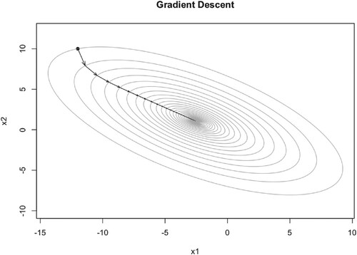
Figure 3. Illustration of GD iteration trajectory with learning rate 0.1.

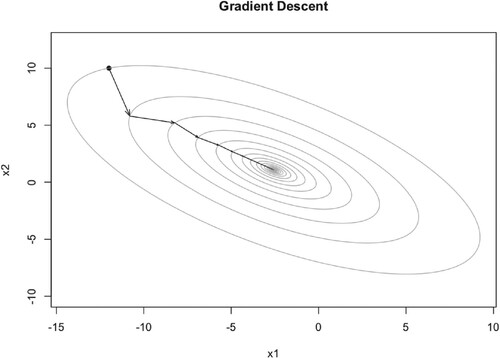
Figure 4. Illustration of GD iteration trajectory with learning rate 0.12.

The learning rates above all are constant. Actually we can use alterable learning rate during iteration. The optimal gradient descent (OGD) is an effective method if the function is not difficult.

We start from any $x_1$, set (4) $x_{k+1}=x_k-{\alpha }_k\mathrm{\nabla }f\left(x_k\right),k=1,2,\dots .$(4) Then (5) $\begin{array}{rl}{\alpha }_k& =\underset{\alpha ⩾0}{\mathrm{a}\mathrm{r}\mathrm{g}\mathrm{m}\mathrm{i}\mathrm{n}}f(x_k-\alpha \mathrm{\nabla }f(x_k\left)\right)\\ & =\frac{{\left[\mathrm{\nabla }f\left(x_k\right)\right]}^{\mathrm{T}}\mathrm{\nabla }f\left(x_k\right)}{{\left[\mathrm{\nabla }f\left(x_k\right)\right]}^{\mathrm{T}}A\mathrm{\nabla }f\left(x_k\right)}.\end{array}$(5) Equation (5(5) $\begin{array}{rl}{\alpha }_k& =\underset{\alpha ⩾0}{\mathrm{a}\mathrm{r}\mathrm{g}\mathrm{m}\mathrm{i}\mathrm{n}}f(x_k-\alpha \mathrm{\nabla }f(x_k\left)\right)\\ & =\frac{{\left[\mathrm{\nabla }f\left(x_k\right)\right]}^{\mathrm{T}}\mathrm{\nabla }f\left(x_k\right)}{{\left[\mathrm{\nabla }f\left(x_k\right)\right]}^{\mathrm{T}}A\mathrm{\nabla }f\left(x_k\right)}.\end{array}$(5) ) is the OGD learning rate.

From Figure 5, we can see that the OGD algorithm converges to the optimal point $x^{\ast }=(-2.5714,1.0857)$, and the number of iteration steps is 41.

Figure 5. Illustration of OGD iteration trajectory.

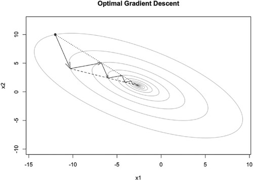
There are some properties of OGD algorithm with quadratic function. We can find that $\overline{x_1{x}_3}$, $\overline{x_3{x}_5}$ etc. are maybe in one line (dotted lines in Figure 5). The same for the dashed lines. If it is true, then we can accelerate GD algorithm. We will discuss it later.

2.2. Polyak momentum algorithm

The learning scheme of the general gradient descent can be very slow sometime. The addition of a momentum term has been found to increase the rate of convergence dramatically, see Qian (1999). With this method, (1(1) $x_i=x_{i-1}-\alpha \mathrm{\nabla }f\left(x_{i-1}\right),$(1) ) takes the form (6) $x_i=x_{i-1}-\alpha \mathrm{\nabla }f\left(x_{i-1}\right)+\mu (x_{i-1}-x_{i-2}),$(6) for $i=3,4,\dots$.

If $\mu \in [0,1]$ and $\alpha >0$ in (6(6) $x_i=x_{i-1}-\alpha \mathrm{\nabla }f\left(x_{i-1}\right)+\mu (x_{i-1}-x_{i-2}),$(6) ), we call it Polyak momentum (PM) algorithm. PM algorithm is also called heavy-ball method in some literatures, see Polyak (1964). Here μ is the momentum parameter. That is, the modification of the vector at the current time step depends on both the current gradient and the change of the previous step. Intuitively, the rationale for using the momentum term is that the GD algorithm is particularly slow when the error function surface is a very long and narrow valley. In this situation, the gradient direction of the GD algorithm is almost perpendicular to the long axis of the valley. This causes the iteration to oscillate back and forth in the short axis while moving very slowly in the long axis of the valley. Rumelhart and McClelland (1986) also showed the momentum term helps average out the oscillation along the short axis while at the same time adds up contributions along the long axis.

We can also show PM algorithm iteration trajectory with different momentum parameter μ. When $\mu =0$, PM algorithm is GD algorithm. That is to say, the GD algorithm is just a special case of PM algorithm.

As we can see, when μ is small, for example $\mu =0.25$, PM algorithm converges to the optimal point $x^{\ast }=(-2.5714,1.0857)$ very fast, see Figure 6. But when μ becomes larger, it converges to the optimal point slowly. However, the iteration points always cross the optimal point, see Figures 7 and 8. The dashed arrow starts from initial point and we can not use the momentum parameter at this time. The number of iteration steps are given in Tables 1–3, which will be discussed later.

Figure 6. Illustration of PM iteration trajectory with $\alpha =0.1$ and $\mu =0.25$.

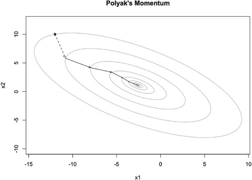
Figure 7. Illustration of PM iteration trajectory with $\alpha =0.1$ and $\mu =0.5$.

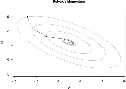
Figure 8. Illustration of PM iteration trajectory with $\alpha =0.1$ and $\mu =0.75$.

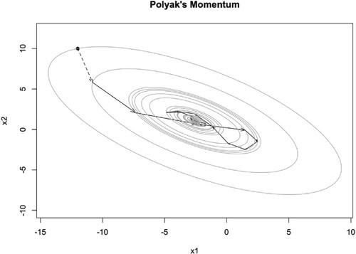
Table 1. Iteration steps of PM, NAG, and TAG algorithms with learning rate $\alpha =0.05$, while the steps of GD algorithm is 117.

μ	PM	NAG	TAG
0.25	79	84	45
0.5	46	37	36
0.75	100	69	30
1	Divergent	190	59

Table 2. Iteration steps of PM, NAG, and TAG algorithms with learning rate $\alpha =0.1$, while the steps of GD algorithm is 54.

μ	PM	NAG	TAG
0.25	26	36	20
0.5	47	49	15
0.75	108	118	25
1	Divergent	Divergent	56

Table 3. Iteration steps of PM, NAG, and TAG algorithms with learning rate $\alpha =0.12$, while the steps of GD algorithm is 44.

μ	PM	NAG	TAG
0.25	24	181	16
0.5	46	Divergent	11
0.75	108	Divergent	7
1	Divergent	Divergent	11

2.3. Nesterov accelerated gradient algorithm

PM algorithm may diverge for relatively simple convex optimisation problems. Mitliagkas (2018) presented an example as follows.

Let f be defined by its gradient as $\mathrm{\nabla }f\left(x\right)=\left\{\begin{array}{ll}25x,& \mathrm{i}\mathrm{f}x<1;\\ x+24,& \mathrm{i}\mathrm{f}1⩽x<2;\\ 25x-24,& \mathrm{o}\mathrm{t}\mathrm{h}\mathrm{e}\mathrm{r}\mathrm{w}\mathrm{i}\mathrm{s}\mathrm{e}.\end{array}\right.$The proof revolves around the idea that the iterations are stuck in a limit cycle. The following subseries of the iterations tend to three points that are not the optimal value of f. $x_{3n}\to p,x_{3n+1}\to q,x_{3n+2}\to r.$They show that $p\approx 0.65$, $q\approx -1.80$, and $r\approx 2.12$.

Leveraging the idea of momentum introduced by Polyak, Nesterov solved that problem by finding an algorithm achieving acceleration the same as the PM algorithm, but that can converge for general convex functions. Nesterov gave the Nesterov accelerated gradient (NAG) algorithm in Nesterov (1983), for $i=3,4,\dots$, the main iteration steps of it are (7) $\begin{array}{l}{y}_i=x_{i-1}-\alpha \mathrm{\nabla }f\left(x_{i-1}\right),\\ x_i=y_i+\mu (y_i-y_{i-1}).\end{array}$(7) The main difference between PM algorithm and NAG algorithm comes from the fact that the latter has two sister sequences working together to produce a corrective movement. Comparing with (6(6) $x_i=x_{i-1}-\alpha \mathrm{\nabla }f\left(x_{i-1}\right)+\mu (x_{i-1}-x_{i-2}),$(6) ), we see that PM algorithm evaluates the gradient before adding momentum, while NAG algorithm evaluates the gradient after applying momentum.

We show NAG algorithm iteration trajectory with different values of momentum parameter μ in Figures 9–11. When $\mu =0$, like PM algorithm, NAG algorithm is GD algorithm.

Figure 9. Illustration of NAG iteration trajectory with $\alpha =0.1$ and $\mu =0.25$.

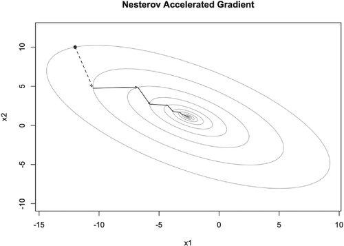
Figure 10. Illustration of NAG iteration trajectory with $\alpha =0.1$ and $\mu =0.5$.

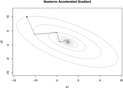
Figure 11. Illustration of NAG iteration trajectory with $\alpha =0.1$ and $\mu =0.75$.

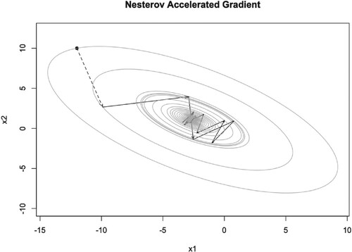
When μ is small, for example $\mu =0.25$ or $\mu =0.5$, NAG algorithm converges to the optimal point $x^{\ast }=(-2.5714,1.0857)$ very fast, see Figures 9–10. But when μ becomes larger, it converges to the optimal point slow down, the iteration points always cross the optimal point, see Figure 11. The dashed arrow starts from the initial point and we can not use the momentum parameter at this time. The number of iteration steps are given in Tables 1–3. We will discuss them later.

2.4. Three-step accelerated gradient algorithm

If the dotted lines $\overline{x_1{x}_3}$, $\overline{x_3{x}_5}$ etc. in Figure 5 are in one line, or the dashed lines $\overline{x_2{x}_4}$, $\overline{x_4{x}_6}$ etc. are in one line, then we can also accelerate GD algorithm. Because they all point to the optimal point. Actually they are in one line, we prove this in Theorem 2.1.

Theorem 2.1

Three-step Accelerated Gradient Algorithm for Two-dimensional Quadratic Function

Assume that A is symmetric and positive definite $(x^{\mathrm{T}}Ax>0$ for any $x\ne 0)$. Consider the two-dimensional quadratic function (8) $f\left(x\right)=\frac{1}{2}{x}^{\mathrm{T}}Ax+b^{\mathrm{T}}x+c,$(8) with the optimal gradient descent iteration and line search, we need only three steps to get to the optimal point.

Proof.

From (8(8) $f\left(x\right)=\frac{1}{2}{x}^{\mathrm{T}}Ax+b^{\mathrm{T}}x+c,$(8) ), we can get $\mathrm{\nabla }f\left(x\right)=Ax+b.$Let $\phi \left(\alpha \right)=f\left(x_{k+1}\right)=f(x_k-\alpha \mathrm{\nabla }f(x_k\left)\right).$Then ${\phi }^{\prime }\left(\alpha \right)=-\left[\mathrm{\nabla }f\right(x_{k+1}\left){]}^{\mathrm{T}}\mathrm{\nabla }f\right(x_k).$Because for the optimal gradient descent, ${\phi }^{\prime }\left(\alpha \right)=0$, so $\left[\mathrm{\nabla }f\right(x_{k+1}\left){]}^{\mathrm{T}}\mathrm{\nabla }f\right(x_k)=0,$that is, $(A{x}_{k+1}+b{)}^{\mathrm{T}}(A{x}_k+b)=0.$Let $x^{\ast }$ be the optimal point, then $x^{\ast }=x_k-A^{-1}(A{x}_k+b),$so $\begin{array}{rl}{x}_k-x^{\ast }& =A^{-1}(A{x}_k+b),\\ x_{k+1}-x^{\ast }& =A^{-1}(A{x}_{k+1}+b).\end{array}$Then $\begin{array}{rl}& (x_{k+1}-x^{\ast }{)}^{\mathrm{T}}{A}^2(x_k-x^{\ast })\\ & =(A{x}_{k+1}+b{)}^{\mathrm{T}}{A}^{-1}{A}^2{A}^{-1}(A{x}_k+b)\\ & =(A{x}_{k+1}+b{)}^{\mathrm{T}}(A{x}_k+b)\\ & =0.\end{array}$Similarly, $(x_{k+2}-x^{\ast }{)}^{\mathrm{T}}{A}^2(x_{k+1}-x^{\ast })=0.$Let $Q=A^2$. When $f:{\mathbb{R}}^2\to \mathbb{R},Q:2\times 2,$we have $\begin{array}{rl}& (x_{k+2}-x^{\ast }{)}^{\mathrm{T}}[Q(x_{k+1}-x^{\ast })]=0,\\ & \left[Q\right(x_{k+1}-x^{\ast }\left){]}^{\mathrm{T}}\right(x_k-x^{\ast })=0.\end{array}$So both $x_{k+2}-x^{\ast }$ and $x_k-x^{\ast }$ are orthogonal to $Q(x_{k+1}-x^{\ast })$.

Because $x^{\ast }$ is the optimal point, so $x_{k+2}-x^{\ast }$ and $x_k-x^{\ast }$ are in the same one dimension subspace. Thus they must be in one line.

Let k = 1, with the direction $x_3-x_1$ and line search, we can approach $x^{\ast }$ at $x_4$. So we need only three steps to get to the optimal point. Thus the result holds.

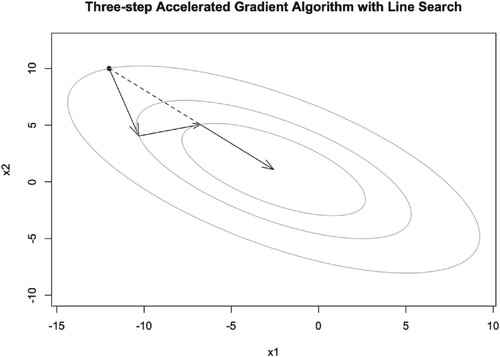
We show the three-step accelerated gradient (TAG) algorithm iteration trajectory for the two-dimensional quadratic function in Figure 12. For the line search of last step, we use the R language package ‘pracma’ which was developed by Borchers (2019).

Figure 12. Illustration of TAG iteration trajectory for two-dimensional quadratic function with line search.

Armijo gave three theorems in Armijo (1966) to illustrate the convergence of the GD algorithm. With the Lipschitz condition in the theorems, we can explain why the algorithms always converge when the learning rate α is small, and will diverge when the learning rate is large.

When the target function is very complex, such as the error function in deep learning, line search may take much time and we still need lots of three-steps to get to the optimal point. So at this time, we use a momentum parameter μ instead of using line search. And based on parallel tangent method proposed by Petalas and Vrahatis (2004), we give TAG algorithm as follows.

The main difference between NAG algorithm and TAG algorithm comes from the fact that the latter has three sequences working together to produce a corrective movement. And based on the idea of Petalas and Vrahatis (2004), the TAG algorithm has more advantages to find out the global optimal value.

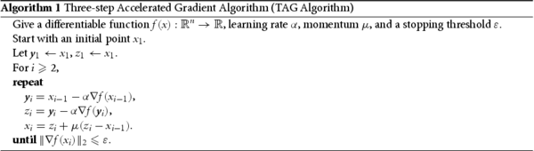
We show the TAG algorithm iteration trajectory with different momentum parameter μ in Figures 13–16. When $\mu =0$, just like the above two algorithms, TAG algorithm is GD algorithm.

Figure 13. Illustration of TAG iteration trajectory with $\alpha =0.1$ and $\mu =0.25$.

Figure 14. Illustration of TAG iteration trajectory with $\alpha =0.1$ and $\mu =0.5$.

Figure 15. Illustration of TAG iteration trajectory with $\alpha =0.1$ and $\mu =0.75$.

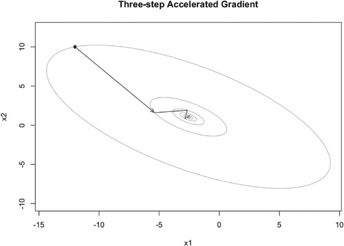
Figure 16. Illustration of TAG iteration trajectory with $\alpha =0.1$ and $\mu =1$.

When $\mu =0.25$, $\mu =0.5$, and $\mu =0.75$, TAG algorithm converges to the optimal point $x^{\ast }=(-2.5714,1.0857)$ very fast, see Figures 13–15. But when μ becomes larger, it converges to the optimal point slowly, the iteration points always cross the optimal point, see Figure 16. But unlike PM algorithm and NAG algorithm, even when $\mu =1$, TAG algorithm always converges to the optimal point. The number of iteration steps are given in Tables 1–3.

From Tables 1–3, we can see that TAG algorithm has more advantages in terms of iteration steps, especially when $\alpha =0.1$ and $\alpha =0.12$. There have two main reasons. One is that the TAG algorithm has three sequences working together to produce a corrective movement. The other reason is that the objective function is a two-dimensional quadratic function, then Theorem 2.1 shows that the TAG algorithm has more advantages. Furthermore, TAG algorithm is more robust than PM and NAG algorithms, for the latter two algorithms always diverge when $\mu =1$. In order to compare the four algorithms further, we give the following two cases.

2.5. Case studies

In order to compare above four algorithms, GD algorithm, PM algorithm, NAG algorithm, and TAG algorithm, we use two kinds of function to implement, i.e. a high dimension quadratic function and a high dimension nonquadratic function. The symmetric and positive definite matrix A of the quadratic function comes from the R language package ‘pracma’ which was developed by Borchers (2019). All kinds of high-dimensional quadratic function can be generated by this package. For nonquadratic function, FLETCHCR function is used, which comes from CUTE (constrained and unconstrained testing environments, from Association for Computing Machinery) collection (Andrei, 2008).

2.5.1. Quadratic function

Tables 4–6 are the iteration steps and runtime for 10-, 100-, and 500-dimensional quadratic functions. The runtime in ‘second’ is within parentheses. The first row is the value of learning rate α. The sign of ‘–’ means this algorithm is diverging during this scenario.

Table 4. Iteration steps and runtime (within parentheses) of 10-dimensional quadratic function.

	GD			PM			NAG			TAG
μ	0.0025	0.005	0.0075	0.0025	0.005	0.0075	0.0025	0.005	0.0075	0.0025	0.005	0.0075
0.2				442	215	140	445	218	143	232	114	74
				(0.0177)	(0.0136)	(0.0136)	(0.0065)	(0.0060)	(0.0059)	(0.0064)	(0.0060)	(0.0061)
0.4				322	151	94	328	158	101	198	96	63
				(0.0126)	(0.0107)	(0.0105)	(0.0055)	(0.0055)	(0.0051)	(0.0054)	(0.0050)	(0.0052)
0.6	559	276	181	193	74	67	204	86	53	172	83	54
	(0.0213)	(0.0261)	(0.0197)	(0.0068)	(0.0104)	(0.0050)	(0.0140)	(0.0055)	(0.0135)	(0.0056)	(0.0051)	(0.0052)
0.8				146	146	146	115	97	97	152	73	47
				(0.0065)	(0.0208)	(0.0252)	(0.0058)	(0.0079)	(0.0063)	(0.0057)	(0.0054)	(0.0057)
1.0				–	–	–	903	491	345	136	65	63
				(–)	(–)	(–)	(0.0071)	(0.0066)	(0.0062)	(0.0056)	(0.0057)	(0.0057)

Table 5. Iteration steps and runtime (within parentheses) of 100-dimensional quadratic function.

	GD			PM			NAG			TAG
μ	0.0025	0.005	0.0075	0.0025	0.005	0.0075	0.0025	0.005	0.0075	0.0025	0.005	0.0075
0.2				1647	819	542	1650	821	545	860	428	284
				(0.0719)	(0.0182)	(0.0207)	(0.0435)	(0.0179)	(0.0147)	(0.0423)	(0.0182)	(0.0154)
0.4				1228	606	398	1233	611	404	736	366	243
				(0.0262)	(0.0166)	(0.0127)	(0.0262)	(0.0165)	(0.0132)	(0.0291)	(0.0172)	(0.0130)
0.6	2065	1029	684	802	386	247	810	395	256	643	319	211
	(0.0551)	(0.0634)	(0.0474)	(0.0198)	(0.0125)	(0.0104)	(0.0199)	(0.0128)	(0.0110)	(0.0252)	(0.0157)	(0.0124)
0.8				343	156	156	356	130	122	571	283	187
				(0.0116)	(0.0098)	(0.0094)	(0.0118)	(0.0089)	(0.0089)	(0.0211)	(0.0142)	(0.0125)
1.0				–	–	–	3680	1898	1219	513	254	168
				(–)	(–)	(–)	(0.0551)	(0.0323)	(0.0430)	(0.0200)	(0.0135)	(0.0116)

Table 6. Iteration steps and runtime (within parentheses) of 500-dimensional quadratic function.

	GD			PM			NAG			TAG
μ	0.0025	0.005	0.0075	0.0025	0.005	0.0075	0.0025	0.005	0.0075	0.0025	0.005	0.0075
0.2				4048	2019	1343	4051	2022	1345	2110	1053	701
				(1.3008)	(0.6927)	(0.5005)	(1.2367)	(0.6920)	(0.5054)	(1.2804)	(0.6994)	(0.5146)
0.4				3028	1506	999	3033	1511	1004	1808	902	600
				(0.9363)	(0.5527)	(0.4361)	(0.9710)	(0.5611)	(0.4216)	(1.1165)	(0.6524)	(0.4869)
0.6	5066	2530	1684	2002	987	648	2010	995	657	1581	788	524
	(1.5307)	(0.8515)	(0.6152)	(0.7105)	(0.4485)	(0.3385)	(0.6991)	(0.4296)	(0.3717)	(0.9993)	(0.5811)	(0.4517)
0.8				950	436	258	961	450	274	1404	700	465
				(0.4423)	(0.3022)	(0.2529)	(0.4228)	(0.2773)	(0.2120)	(0.9032)	(0.5412)	(0.4373)
1.0				–	–	–	9836	4797	3168	1263	629	418
				(–)	(–)	(–)	(2.7888)	(1.4743)	(1.0167)	(0.8557)	(0.5045)	(0.4282)

Tables 4–6 show that with respect to both iteration steps and runtime, TAG algorithm is superior to NAG algorithm, NAG algorithm is superior to PM algorithm, PM algorithm is superior to GD algorithm. And with the momentum parameter μ, we can find out that TAG is more robust than NAG, NAG is more robust than PM. Notice that when $\mu =1$, PM is always diverging. The larger learning rate α, the fewer the iteration steps and the less runtime needed. But too large learning rate will lead to divergency of algorithms. When μ changes from 0 to 1, the iteration steps and runtime decrease then increase, so there may exist an optimal μ for PM, NAG and TAG algorithms. The momentum parameter μ of TAG algorithm can be larger than 1. Next, we implement these four algorithms to the FLETCHCR function and compare them.

2.5.2. FLETCHCR function

The FLETCHCR function is given as follows, which comes from CUTE collection. (9) $\begin{array}{r}f\left(x\right)=\sum _{i=1}^{n-1}C(x_{i+1}-x_i+1-x_i^2{)}^2,\\ x_0=(0,0,\dots ,0),\\ C=100.\end{array}$(9)

Tables 7–9 demonstrate the iteration steps, runtime, and optimal μ with its range for 10-, 100-, and 500-dimensional FLETCHCR functions. The runtime in ‘second’ is within parentheses. The range of μ is within brackets with optimal value on the left.

Table 7. Iteration steps, runtime (within parentheses), and optimal μ with its range (within brackets) for 10-dimensional FLETCHCR function.

α	GD		PM			NAG			TAG
0.0007	151	(0.0261)	41	(0.0191)	0.6[0,0.9]	149	(0.0240)	0.8[0,0.8]	57	(0.0205)	0.3[0,1.5]
0.0005	210	(0.0223)	55	(0.0235)	0.7[0,0.9]	48	(0.0176)	0.7[0,1]	58	(0.0260)	0.9[0,1.9]
0.0003	343	(0.0310)	78	(0.0215)	0.8[0,0.9]	65	(0.0184)	0.8[0,1]	91	(0.0197)	1[0,2.5]
0.0001	967	(0.0603)	169	(0.0271)	0.9[0,0.9]	138	(0.0496)	0.9[0,1]	131	(0.0272)	3.1[0,6.4]

Table 8. Iteration steps, runtime (within parentheses), and optimal μ with its range (within brackets) for 100-dimensional FLETCHCR function.

α	GD		PM			NAG			TAG
0.0006	329	(0.0950)	358	(0.1079)	0.9[0,0.9]	2412	(0.4783)	0.9[0.7,0.9]	253	(0.1106)	0.1[0,1.4]
0.0005	687	(0.1790)	326	(0.0932)	0.1[0,0.9]	276	(0.1351)	0.2[0,0.3]	183	(0.0835)	0.2[0,1.7]
0.0004	1150	(0.2400)	350	(0.0972)	0.2[0,0.9]	305	(0.1290)	0.3[0,1]	199	(0.0792)	0.4[0,1.8]
0.0003	1799	(0.3785)	420	(0.1229)	0.3[0,0.9]	405	(0.0979)	0.4[0,1]	198	(0.0883)	0.7[0,2.3]
0.0002	2892	(0.5712)	647	(0.1644)	0.4[0,0.9]	633	(0.1498)	0.5[0,1]	240	(0.0966)	1.3[0,1.4]

Table 9. Iteration steps, runtime (within parentheses), and optimal μ with its range (within brackets) for 500-dimensional FLETCHCR function.

α	GD		PM			NAG			TAG
0.0006	1213	(1.1347)	718	(0.6414)	0.7[0,0.9]	4452	(3.7189)	0.9[0.8,0.9]	477	(0.5958)	0.6[0,1.3]
0.0005	2019	(1.6973)	1200	(1.0165)	0.4[0,0.9]	1993	(1.6932)	0.3[0,0.3]	734	(0.8973)	0.8[0,1.4]
0.0004	1997	(1.6917)	998	(0.8588)	0.8[0,0.9]	951	(0.8170)	0.4[0,1]	471	(0.5883)	0.7[0,1.7]
0.0003	5439	(4.5350)	1993	(1.6944)	0.4[0,0.9]	1453	(1.3234)	0.9[0,1]	647	(0.8019)	0.4[0,1]
0.0002	7791	(6.5177)	1449	(1.2472)	0.9[0,0.9]	1205	(1.0455)	1[0,1]	954	(1.1697)	0.9[0,1.3]

From Tables 7–9, we can obtain that compared with NAG, PM and GD algorithms, TAG algorithm has fewer iteration steps and less runtime, and has longer range of μ, which means TAG algorithm is more robust than other algorithms. The optimal value of μ of TAG algorithm can be larger than 1. PM algorithm and NAG algorithm maybe have the similar performance but both are superior to GD algorithm.

3. TAG algorithm in deep learning

3.1. Why use deep learning?

The development history of deep learning can be seen in Mcculloch and Pitts (1990), Hebb (1949), Rumelhart et al. (1986), Hinton and Salakhutdinov (2006) and Krizhevsky et al. (2017). The reason we consider accelerating backpropagation algorithm in deep learning is because deep learning has excellent effects in classification projects, speech recognition, and image processing. This paper mainly studies classification problems. From Matloff (2017) and Hastie et al. (2015), we can see that multinomial logistic regression (MLR) is the most practical and effective way to solve multi-classification problems, which is a generalisation of logistic regression. The MLR model which has K categories is as follows. (10) $\begin{array}{rlr}& P(y=k|x,w)& =\frac{{\mathrm{e}}^{h\left(x|w_k\right)}}{1+\sum _{i=1}^{K-1}{\mathrm{e}}^{h\left(x|w_i\right)}},\end{array}$(10) (11) $\begin{array}{rlr}& P(y=K|x,w)& =\frac{1}{1+\sum _{i=1}^{K-1}{\mathrm{e}}^{h\left(x|w_i\right)}}.\end{array}$(11) here, $h\left(x|w_k\right)=w_{k0}+w_{k1}{x}_1+w_{k2}{x}_2+\cdots +w_{kn}{x}_n$, and $k=1,2,\dots ,K-1$.

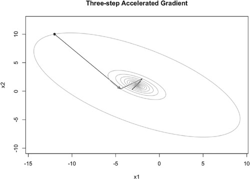
Let us see a spiral data set from the computer science course of Stanford University (Stanford, 2019). For the data size of this data set, the input is $800\times 2$, the output is $800\times 4$, and the output values are divided into 4 categories. The scatter plot of spiral data is given in Figure 17, which is plotted by R language package ‘ggplot2’ developed by Wickham (2016).

Figure 17. The scatter plot of spiral data.

Referring to James et al. (2015), we estimate the coefficients of MLR model using the R language packages ‘nnet’ developed by Ripley and Venables (2020) and ‘tidyverse’ developed by Wickham (2014). The classification accuracy of this model is only 0.3188. Obviously, the classification effect is not good. Hastie et al. (2009) pointed out that Support Vector Machines (SVM) is a very effective classification method in statistical learning. It can change each linearly inseparable problem into a separable one. The main part of SVM model is the following constrained optimisation problem. (12) $\begin{array}{rl}& \underset{w,w_0}{\mathrm{m}\mathrm{i}\mathrm{n}}\left\{\frac{1}{2}\parallel w{\parallel }^2+C\sum _{i=1}^N{\xi }_i\right\},\end{array}$(12) (13) $\begin{array}{rl}& \mathrm{s}.\mathrm{t}.{\xi }_i⩾0,y_i\left(x_i^{\mathrm{T}}w+w_0\right)⩾1-{\xi }_i,\\ & i=1,2,\dots ,N.\end{array}$(13) Here N is the sample size, ${\xi }_i$ is the slack variable, and C is the penalty coefficient.

Referring to Karatzoglou and Meyer (2006), we use the R language package ‘e1071’ developed by Meyer et al. (2019) to train the spiral data set with SVM model. Here the selected kernel function is ‘radial’ with a penalty coefficient of C = 5. After training, 547 support vectors are generated and the classification accuracy is 0.9163, which shows that the classification effect is very good.

Finally, we use the R language package ‘supneuralnet’ developed by ourselves to train the spiral data set with deep learning model. This package will be introduced in detail later, it is rewritten from the R language package ‘neuralnet’ which was developed by Fritsch et al. (2019). Here the neural network contains only one hidden layer, and the hidden layer contains 50 neurons. After 6000 iterations, the classification accuracy reaches 0.98, which has exceeded the SVM model.

Statistics at a crossroads: who is for the challenge? He illustrated this in Berger and He (2019). Research in deep learning is ruinously expensive, and the standard algorithms are ridiculously slow to converge. So the accelerated algorithms in deep learning are very necessary.

3.2. Backpropagation with three-step accelerated gradient

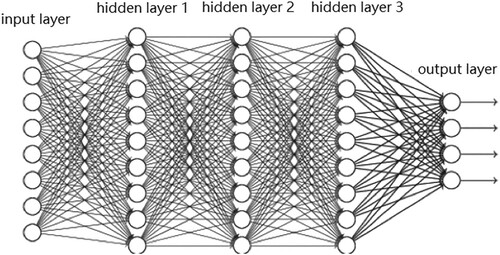
Feedforward neural networks are the first type of artificial neural networks where the connections between neurons do not form a cycle. Feedforward neural networks are simpler than their counterpart, recurrent neural networks. The reason why they are called feedforward is that the information in these networks is only forwarded, do not have loops. The information first through the input neurons, then through the hidden neurons (if present), and finally through the output neurons. In industry and academia, a neural network is called deep learning which has at least one hidden layer. Figure 18 gives the information transmission procedure of a feedforward neural network with 3 hidden layers.

Figure 18. Feedforward neural network with 3 hidden layers.

Throughout the books and literatures on neural networks and deep learning (Anthony & Bartlett, 2009; Blum & Rivest, 1992; Hinton et al., 2006; Hornik, 1991; Kawaguchi, 2016; Prechelt, 1994), the mathematical representations of neural networks are different. The representation in Goodfellow et al. (2016) is very popular. We will combine them and present the mathematical formulas in this paper.

We consider a feedforward neural network has M layers, whose lth layer contains $N_l$ neurons, for $l=1,2,\dots ,M$. $y_j^l$ represents the output of the jth neuron at the lth layer. When l = 1, which is the input layer, we let $y_j^1$ equal to the input vector $v=(v_1,v_2,\dots ,v_{N_1})$ of the input layer, that is (14) $y_j^1=v_j,j=1,2,\dots ,N_1.$(14) For the 2nd layer to the (M−1)th layer, i.e. $2⩽l⩽M-1$, $y_j^l$ is calculated by (15) $\begin{array}{rl}{\mathrm{n}\mathrm{e}\mathrm{t}}_j^l& =b_j^l+\sum _{i=1}^{N_{l-1}}{w}_{ij}^{l-1,l}{y}_i^{l-1},\end{array}$(15) (16) $\begin{array}{rl}{y}_j^l& =f\left({\mathrm{n}\mathrm{e}\mathrm{t}}_j^l\right),\end{array}$(16) where $j=1,2,\dots ,N_l$. Here ${\mathrm{n}\mathrm{e}\mathrm{t}}_j^l$ is the sum of its weighted inputs. $w_{ij}^{l-1,l}$ is the weight from the ith neuron at the (l−1)th layer to the jth neuron at the lth layer. $b_j^l$ is the bias of the jth neuron at the lth layer. $f\left({\mathrm{n}\mathrm{e}\mathrm{t}}_j^l\right)$ is the activation function of the jth neuron at the lth layer. There are many commonly used activation functions, four of them are listed below.

• Sigmoid function (17) $f\left(x\right)=\frac{1}{1+{\mathrm{e}}^{-x}},$(17)

• Tangent function (18) $f\left(x\right)=\tanh \left(x\right),$(18)

• ReLU function (19) $f\left(x\right)=max\{0,x\},$(19)

• Softplus function (20) $f\left(x\right)=\ln (1+{\mathrm{e}}^x).$(20)

The Softplus function is an approximation of the ReLU function. But the Softplus function is a smooth function, which is easy to get the derivative.

For the Mth layer, which is the output layer, $y_j^M$ is calculated by (21) $\begin{array}{rl}& {\mathrm{n}\mathrm{e}\mathrm{t}}_j^M=b_j^M+\sum _{i=1}^{N_{M-1}}{w}_{ij}^{M-1,M}{y}_i^{M-1},\end{array}$(21) (22) $\begin{array}{rl}& y_j^M=f\left({\mathrm{n}\mathrm{e}\mathrm{t}}_j^M\right),\end{array}$(22) where $j=1,2,\dots ,N_M$. We give the formulas of output layer separately because the backpropagation algorithm starts from the output layer in order to minimise the error function. In the following, a combination of numbers is used to represent the structure of a neural network. For example, the neural network in Figure 18 is represented as a 8-9-9-9-4 type neural network.

The backpropagation algorithm was discovered in the 1970s, but the importance of this algorithm was not recognised until Rumelhart, Hinton, and Williams published a paper on Nature (Rumelhart et al., 1986). Backpropagation is short for backward propagation of errors, which is an algorithm for supervised learning of artificial neural networks using gradient descent. It is the most widely used algorithm for training multilayer feedforward neural networks. If an artificial neural network and an error function are given, backpropagation mainly uses the chain rule to calculate the gradient of the error function to weights.

Let the input-output pair of a neural network is $(v,t)$, and the sample size is P, then the error function (or loss function) is (23) $E=\frac{1}{2}\sum _{p=1}^P\sum _{j=1}^{N_M}(y_{j,p}^M-t_{j,p}{)}^2=\sum _{p=1}^P{E}_p,$(23) where the error of the pth sample is (24) $E_p=\frac{1}{2}\sum _{j=1}^{N_M}(y_{j,p}^M-t_{j,p}{)}^2.$(24) For the error function, (23(23) $E=\frac{1}{2}\sum _{p=1}^P\sum _{j=1}^{N_M}(y_{j,p}^M-t_{j,p}{)}^2=\sum _{p=1}^P{E}_p,$(23) ) is divided by P in some literatures. But it has no effect on minimising error function compared with (23(23) $E=\frac{1}{2}\sum _{p=1}^P\sum _{j=1}^{N_M}(y_{j,p}^M-t_{j,p}{)}^2=\sum _{p=1}^P{E}_p,$(23) ), because P is a constant. And there are many kinds of loss function, this is just the most widely used one.

To simplify the mathematical formulas further, the bias $b_j^l$ for the jth neuron at the lth layer will be incorporated into the weights as $w_{0j}^{l-1,l}$ with a fixed output of $y_{0,p}^{l-1}=1$. Thus (25) ${\mathrm{n}\mathrm{e}\mathrm{t}}_{j,p}^l=b_j^l+\sum _{i=1}^{N_{l-1}}{w}_{ij}^{l-1,l}{y}_{i,p}^{l-1}=\sum _{i=0}^{N_{l-1}}{w}_{ij}^{l-1,l}{y}_{i,p}^{l-1}.$(25) In the backpropagation algorithm, minimisation of E is usually using the gradient descent with constant learning rate α, and the computation of $\mathrm{\nabla }E$ by applying the chain rule and product rule in differential calculus. The backpropagation algorithm is mainly how to calculate (26) $\frac{\mathrm{\partial }E}{\mathrm{\partial }{w}_{ij}^{l-1,l}}=\sum _{p=1}^P\frac{\mathrm{\partial }{E}_p}{\mathrm{\partial }{w}_{ij}^{l-1,l}}.$(26) According to the chain rule in differential calculus, we have (27) $\frac{\mathrm{\partial }{E}_p}{\mathrm{\partial }{w}_{ij}^{l-1,l}}=\frac{\mathrm{\partial }{E}_p}{\mathrm{\partial }{\mathrm{n}\mathrm{e}\mathrm{t}}_{j,p}^l}\cdot \frac{\mathrm{\partial }{\mathrm{n}\mathrm{e}\mathrm{t}}_{j,p}^l}{\mathrm{\partial }{w}_{ij}^{l-1,l}}.$(27) Where $\frac{\mathrm{\partial }{\mathrm{n}\mathrm{e}\mathrm{t}}_{j,p}^l}{\mathrm{\partial }{w}_{ij}^{l-1,l}}=\frac{\mathrm{\partial }}{\mathrm{\partial }{w}_{ij}^{l-1,l}}\left(\sum _{k=0}^{N_{l-1}}{w}_{kj}^{l-1,l}{y}_{k,p}^{l-1}\right)=y_{i,p}^{l-1}.$Let (28) ${\delta }_{j,p}^l=\frac{\mathrm{\partial }{E}_p}{\mathrm{\partial }{\mathrm{n}\mathrm{e}\mathrm{t}}_{j,p}^l},$(28) thus (29) $\frac{\mathrm{\partial }{E}_p}{\mathrm{\partial }{w}_{ij}^{l-1,l}}={\delta }_{j,p}^l{y}_{i,p}^{l-1}.$(29) For the Mth layer, we have (30) ${\delta }_{j,p}^M=\frac{\mathrm{\partial }{E}_p}{\mathrm{\partial }{\mathrm{n}\mathrm{e}\mathrm{t}}_{j,p}^M}=\left(y_{j,p}^M-t_{j,p}\right)f^{\mathrm{\prime }}\left({\mathrm{n}\mathrm{e}\mathrm{t}}_{j,p}^M\right).$(30) For the hidden layers, i.e. $2⩽l⩽M-1$, according to Rumelhart et al. 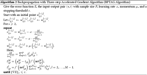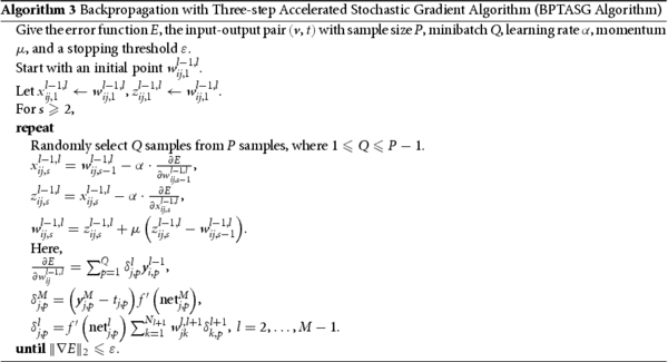(1986), (31) ${\delta }_{j,p}^l=f^{\mathrm{\prime }}\left({\mathrm{n}\mathrm{e}\mathrm{t}}_{j,p}^l\right)\sum _{k=1}^{N_{l+1}}{w}_{jk}^{l,l+1}{\delta }_{k,p}^{l+1}.$(31) Artificial neural networks generally spend a lot of time when training data sets with the backpropagation algorithm. So the acceleration of the backpropagation algorithm is very meaningful. We give the backpropagation with three-step accelerated gradient (BPTAG) algorithm as follows.

3.3. R package supneuralnet

Programming is important after given an algorithm, but the programming of deep learning is difficult. It is relatively easy to program a neural network with only one hidden layer, but this is not versatile, which cannot be used in a neural network with two hidden layers.

R language package ‘neuralnet’ which was developed by Fritsch et al. (2019) is a good package in deep learning. But it only includes the backpropagation with gradient descent (BPGD) algorithm for algorithms in this paper. So we rewrite this package, named ‘supneuralnet’, which includes all algorithms in this paper. In addition to BPGD algorithm, backpropagation with Polyak momentum (BPPM) algorithm, backpropagation with Nesterov accelerated gradient (BPNAG) algorithm, and BPTAG algorithm are added to package ‘supneuralnet’.

The stochastic gradient descent algorithm is also added to package ‘supneuralnet’, then backpropagation with stochastic gradient descent (BPSGD) algorithm, backpropagation with Polyak momentum and stochastic gradient descent (BPPMSGD) algorithm, backpropagation with Nesterov accelerated stochastic gradient (BPNASG) algorithm, and backpropagation with three-step accelerated stochastic gradient (BPTASG) algorithm are automatically added to this package. These will be seen in Section 5.

4. Case studies based on BPTAG algorithm

We apply the BPGD, BPPM, BPNAG, and BPTAG algorithms to two cases, and compare the performances of these algorithms. The purposes of the two cases are different. For iris data set, we control the training accuracy and compare the iteration steps and runtime. For spiral data set, we control the iteration steps and compare the training accuracy. In addition, the performances of linear methods are not bad for iris data set, which can not be accepted for spiral data set.

4.1. Iris data set

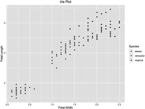
The iris data set is an open source data set in R language (R Core Team, 2020), it has 150 rows and 5 columns. The scatter plot of iris petal is given in Figure 19.

Figure 19. The scatter plot of iris petal.

The ‘supneuralnet’ package is used for training iris data with BPGD, BPPM, BPNAG, and BPTAG algorithms. The data is trained 100 times with the 2-6-3 type neural network for each algorithm, and the optimal one is selected. Figure 20 represents the training results of BPTAG algorithm with learning rate $\alpha =0.05$ and momentum parameter $\mu =0.1$. The processor of machine is 3.1 GHz Dual-Core Intel Core i7 with 16 GB memory. The iteration steps and runtime of algorithms with the values of learning rate and momentum are given in Tables 10–12. The runtime in ‘second’ is within parentheses.

Figure 20. BPTAG algorithm training results of iris data set with $\alpha =0.05$ and $\mu =0.1$.

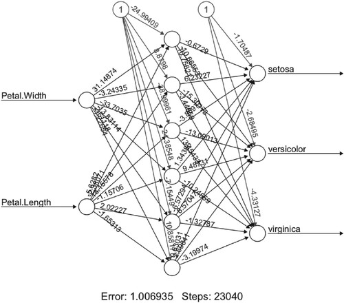
Table 10. Iteration steps and runtime (within parentheses) of BPPM, BPNAG, and BPTAG algorithms with learning rate $\alpha =0.025$ for iris data set, while the steps and runtime of BPGD algorithm are 64822 and 17.88s respectively.

μ	BPPM	BPNAG	BPTAG
0.05	76237 (17.46)	56026 (13.99)	43501 (11.88)
0.1	64836 (16.98)	59333 (15.45)	35833 (10.53)
0.15	57391 (13.95)	69196 (17.92)	27076 (8.98)
0.2	55868 (12.75)	64429 (16.93)	40679 (10.56)

Table 11. Iteration steps and runtime (within parentheses) of BPPM, BPNAG, and BPTAG algorithms with learning rate $\alpha =0.05$ for iris data set, while the steps and runtime of BPGD algorithm is 48849 and 11.77s respectively.

μ	BPPM	BPNAG	BPTAG
0.05	39741 (9.85)	46259 (11.73)	25755 (7.71)
0.1	38682 (9.17)	37256 (8.78)	23040 (6.93)
0.15	38912 (9.53)	45347 (10.91)	19699 (6.18)
0.2	Divergent	33057 (8.01)	20060 (6.22)

Table 12. Iteration steps and runtime (within parentheses) of BPPM, BPNAG, and BPTAG algorithms with learning rate $\alpha =0.075$ for iris data set, while the steps and runtime of BPGD algorithm is 33503 and 8.09s respectively.

μ	BPPM	BPNAG	BPTAG
0.05	33582 (8.05)	39123 (9.33)	17979 (6.08)
0.1	27066 (6.85)	38918 (9.32)	18189 (6.53)
0.15	29095 (7.08)	32257 (8.18)	16477 (5.29)
0.2	29165 (7.29)	24596 (6.24)	14982 (4.96)

It can be seen from the three tables that the BPPM, BPNAG, and BPTAG algorithms are better than the BPGD algorithm. If α is too large, then it will lead to divergency of algorithms. If α is too small, then it will lead to more iteration steps and runtime of algorithms. The momentum parameter μ has similar variation tendency. This is consistent with the variation tendencies of learning rate and momentum of GD, PM, NAG, and TAG algorithms in Section 2. In fact, during the 100 times training process in Table 12, some trainings of these algorithms are divergent. Taken together, BPTAG algorithm is better than BPPM and BPNAG algorithms, and it is more robust to momentum parameter μ. Because BPTAG algorithm is still convergent when μ becomes larger. The BPPM algorithm has the similar iteration steps and runtime to the BPNAG algorithm, but the BPNAG algorithm is more robust, because the BPPM algorithm is more likely to diverge when μ becomes larger.

4.2. Spiral data set

The spiral data set has been introduced in Section 3, which can not be classified with the linear models. In this case, the softmax loss function is chosen to train the data, thus (32) $E_p=-\sum _{j=1}^{N_M}\ln \left(\frac{{\mathrm{e}}^{y_{j,p}^M}}{\sum _{k=1}^P{\mathrm{e}}^{y_{j,k}^M}}\right).$(32) In order to avoid overfitting, the $L2$ regularisation is added to E. Therefore the loss function becomes (33) $\begin{array}{rl}E& =-\sum _{p=1}^P\sum _{j=1}^{N_M}\ln \left(\frac{{\mathrm{e}}^{y_{j,p}^M}}{\sum _{k=1}^P{\mathrm{e}}^{y_{j,k}^M}}\right)\\ & +\frac{\lambda }{2}\sum _{l=2}^M\sum _{i=1}^{N_{l-1}}\sum _{j=1}^{N_l}{\left(w_{ij}^{l-1,l}\right)}^2.\end{array}$(33) Where λ is the regularisation parameter.

The spiral data set is trained by BPGD, BPPM, BPNAG, and BPTAG algorithms with ReLU activation function. The number of iteration steps is set to 3000 steps with regularisation parameter $\lambda =0.0002$ for all algorithms. The data is trained 100 times with the 2-50-4 type neural network for each algorithm, and the optimal one is selected. The training accuracy of algorithms with the values of learning rate α and momentum μ are given in Tables 13–15.

Table 13. Training accuracy of BPPM, BPNAG, and BPTAG algorithms with learning rate $\alpha =0.25$ for spiral data set, while the accuracy of BPGD algorithm is 0.8775.

μ	BPPM	BPNAG	BPTAG
0.25	0.9137	0.9162	0.9775
0.5	0.9625	0.9487	0.9725
0.75	0.9812	0.9225	0.9787
1	0.2500	0.7187	0.9800

Table 14. Training accuracy of BPPM, BPNAG, and BPTAG algorithms with learning rate $\alpha =0.5$ for spiral data set, while the accuracy of BPGD algorithm is 0.8950.

μ	BPPM	BPNAG	BPTAG
0.25	0.9650	0.9175	0.9825
0.5	0.9750	0.9812	0.9821
0.75	0.9675	0.9750	0.9862
1	0.2500	0.3725	0.9900

Table 15. Training accuracy of BPPM, BPNAG, and BPTAG algorithms with learning rate $\alpha =0.75$ for spiral data set, while the accuracy of BPGD algorithm is 0.8975.

μ	BPPM	BPNAG	BPTAG
0.25	0.9462	0.9662	0.9875
0.5	0.9862	0.9712	0.9337
0.75	0.9850	0.9875	0.9800
1	0.2500	0.2500	0.9900

It can be seen from the three tables that the four algorithms have the highest accuracy when $\alpha =0.75$. As the learning rate α decreases to 0.5, and then to 0.25, the training accuracy of the four algorithms decreases slowly. If momentum μ is too large or too small, then it will lead to lower accuracy for BPPM and BPNAG algorithms. In particular, the training accuracy of BPPM algorithm is 0.25 when $\mu =1$, which means that it classifies all the training data into one class. And the training accuracy of BPNAG algorithm is 0.25 occasionally when $\mu =1$, it is very low. At the same time, the training accuracy of the BPTAG algorithm is particularly high, even reaching 0.99, which is a great advantage. Once again, this proves that the BPTAG algorithm is more robust than BPPM and BPNAG algorithms for the momentum parameter μ. In general, the performances of the four algorithms are still the same as the iris data set. The BPTAG algorithm has the highest training accuracy, the BPGD algorithm has the lowest training accuracy, and the training accuracy of BPPM algorithm and BPNAG algorithm is almost the same.

5. Three-step accelerated stochastic gradient algorithm in deep learning

5.1. Backpropagation with three-step accelerated stochastic gradient

The gradient descent algorithm needs to use all the data in each iteration during training, which brings challenges to solve the optimisation problems of large scale data. Given an artificial neural network, in order to update the weights, the BPGD algorithm needs to use all the training data every time. When P is large, it requires lots of computational resources and computing time, which is not feasible in the actual production process. So the stochastic gradient descent (SGD) algorithm is proposed to solve this problem.

The SGD algorithm is to use the minibatch data instead of all data to calculate the gradient every time. That is to say, SGD algorithm randomly selects Q samples from P samples when calculating the gradient in each iteration, where $1⩽Q⩽P-1$.

In practical application, parameter tuning is used to obtain the optimal Q. Generally, it can take full advantage of matrix operation in the computer program when $Q=2^n$, such as 16, 32, 64, 128, 256, and so on.

Since the backpropagation with stochastic gradient descent (BPSGD) algorithm uses part of the data set in each iteration, it should take more iteration steps to converge. So the acceleration of BPSGD algorithm is very helpful for the big data computing. BPSGD algorithm, backpropagation with Polyak momentum and stochastic gradient descent (BPPMSGD) algorithm, backpropagation with Nesterov accelerated stochastic gradient (BPNASG) algorithm, and backpropagation with three-step accelerated stochastic gradient (BPTASG) algorithm have been added to the R language package ‘supneuralnet’, see Section 3. The BPTASG algorithm is given as follows.

5.2. Iris data set

The ‘supneuralnet’ package is used for training iris data with BPSGD, BPPMSGD, BPNASG, and BPTASG algorithms. The data is trained 100 times with the 2-6-3 type neural network and minibatch Q = 64 for each algorithm, and the optimal one is selected. According to the results of Section 4, we choose learning rate $\alpha =0.05$. Figure 21 represents the training results of BPTASG algorithm with momentum parameter $\mu =0.1$. The iteration steps and runtime of algorithms with the value of momentum are given in Table 16. The runtime in ‘second’ is within parentheses.

Figure 21. BPTASG algorithm training results of iris data set with $\alpha =0.05$ and $\mu =0.1$.

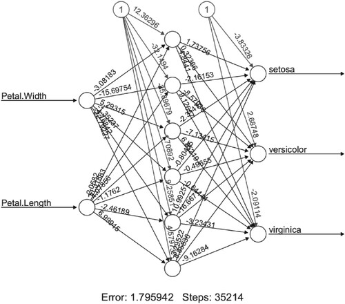
Table 16. Iteration steps and runtime (within parentheses) of BPPMSGD, BPNASG, and BPTASG algorithms with learning rate $\alpha =0.05$ for iris data set, while the steps and runtime of BPSGD algorithm is 123859 and 22.13s respectively.

μ	BPPMSGD	BPNASG	BPTASG
0.05	75929 (14.67)	54308 (12.31)	32059 (12.04)
0.1	54614 (13.98)	67163 (14.99)	35214 (13.45)
0.15	46414 (12.48)	83250 (17.54)	43917 (16.11)
0.2	62638 (14.18)	50136 (11.74)	27907 (10.36)

Compared with Table 11, it can be seen that the BPSGD algorithm requires 123859 steps to converge, which is 2.5 times the iteration steps of BPGD algorithm. At the same time, BPSGD algorithm requires 22.13 seconds to converge, which is about 2 times the runtime of BPGD algorithm. The iteration steps required by accelerated algorithms are almost twice the iteration steps of using the full data set. Some are just less than two times, such as the BPTASG algorithm with momentum $\mu =0.05$. The runtime required by accelerated algorithms are almost 1.5 times the runtime of using the full data set. This shows that the accelerated algorithms have really nice effects, and the BPPMSGD algorithm also converges when $\mu =0.2$. In general, too large momentum μ or too small momentum μ will lead to more iteration steps and runtime for BPPMSGD, BPNASG, and BPTASG algorithms. The BPTASG algorithm has the least iteration steps and runtime, the BPSGD algorithm has the most iteration steps and runtime, and BPPMSGD algorithm and BPNASG algorithm are almost the same.

5.3. Spiral data set

According to the results of Section 4, we choose learning rate $\alpha =0.5$. The spiral data set is trained by BPSGD, BPPMSGD, BPNASG, and BPTASG algorithms with ReLU activation function, softmax loss function, and the $L2$ regularisation. The number of iteration steps is set to 3000 steps with regularisation parameter $\lambda =0.0002$ for all algorithms. The data is trained 100 times with the 2-50-4 type neural network and minibatch Q = 128 for each algorithm, and the optimal one is selected. The training accuracy of algorithms with the value of momentum μ is given in Table 17.

Table 17. Training accuracy of BPPMSGD, BPNASG, and BPTASG algorithms with learning rate $\alpha =0.5$ for spiral data set, while the accuracy of BPSGD algorithm is 0.8887.

μ	BPPMSGD	BPNASG	BPTASG
0.25	0.9475	0.9162	0.9662
0.5	0.9262	0.9750	0.9762
0.75	0.9037	0.9450	0.9787
1	0.2500	0.3075	0.9575

Compared with the Table 14, we find out that with only 3000 iterations, the SGD algorithm reduces the training accuracy. Actually, it needs more iteration steps to reach the training accuracy in Table 14. But the runtime is much shorter after adding the SGD algorithm, and the accuracy is high enough. It can be seen from Table 17 that too large momentum μ or too small momentum μ will lead to lower accuracy for accelerated algorithms. In particular, the training accuracy of BPPMSGD algorithm is 0.25 when $\mu =1$, which means that it classifies all the training data into one class. And the training accuracy of BPNASG algorithm is 0.3075 at this time, which is very low. While the training accuracy of the BPTASG algorithm is very high, which is a great advantage. This proves that the BPTASG algorithm is more robust than BPPMSGD and BPNASG algorithms for the momentum parameter μ. Overall, BPTASG algorithm is superior to BPNASG algorithm, BPNASG algorithm is superior to BPPMSGD algorithm, and BPPMSGD algorithm is superior to BPSGD algorithm.

6. Conclusion

This paper proposes the TAG algorithm and applies it to deep learning. Firstly, we introduce GD algorithm, and give the applications of it to a quadratic function, then state PM and NAG algorithms, give the TAG algorithm, and implement them to the quadratic function. The paper conducts experiments to high-dimensional functions that help us to understand TAG with the fastest convergence among these four algorithms. Secondly, we introduce deep learning and backpropagation algorithm. Then the TAG algorithm is added to the backpropagation algorithm. Since the R language package ‘neuralnet’ only contains the GD algorithm of the algorithms in this paper, we rewrite the ‘neuralnet’ package, named ‘supneuralnet’. The PM algorithm, NAG algorithm, and TAG algorithm are added. We also add the SGD algorithm, so that SGD and other algorithms can be combined with freedom. Thirdly, we apply the four algorithms to the iris and spiral data sets in the deep learning framework, compare their classification effects and convergence speed. We find out that our algorithm is the best. Finally, we combine the SGD algorithm with the above four algorithms, and apply them to the iris and spiral data sets in the deep learning framework, compare their classification effects and convergence speed. We also find out that our algorithm is the best. Moreover, we can do more research for the scalability of BPTASG algorithm with more datasets in the future. The theoretical convergence analysis of BPTASG algorithm is also well worth studying.

Disclosure statement

No potential conflict of interest was reported by the author(s).

Additional information

Funding

This work was supported by National Natural Science Foundation of China (11271136, 81530086), Program of Shanghai Subject Chief Scientist (14XD1401600) and the 111 Project of China (No. B14019).

Notes on contributors

Yongqiang Lian

Yongqiang Lian is a Ph.D. candidate in Statistics at East China Normal University.

Yincai Tang

Yincai Tang is a Professor in School of Statistics at East China Normal University.

Shirong Zhou

Shirong Zhou is a Ph.D. student in Statistics at East China Normal University.

References

- Andrei, N. (2008). An unconstrained optimization test functions collection. Advanced Modeling and Optimization, 10(1), 147–161.
- Anthony, M., & Bartlett, P. L. (2009). Neural network learning: Theoretical foundations. Cambridge University Press.
- Armijo, L. (1966). Minimization of functions having Lipschitz continuous first partial derivatives. Pacific Journal of Mathematics, 16(1), 1–3. https://doi.org/https://doi.org/10.2140/pjm
- Berger, J., & He, X. (2019). Statistics at a crossroads: Challenges and opportunities in the data science era. https://hub.ki/groups/statscrossroad/overview.
- Bishop, C. M. (Ed.). (2006). Pattern recognition and machine learning. Springer.
- Blum, A. L., & Rivest, R. L. (1992). Training a 3-node neural network is NP-complete. Neural Networks, 5(1), 117–127. https://doi.org/https://doi.org/10.1016/S0893-6080(05)80010-3
- Borchers, H. W. (2019). pracma: Practical numerical math functions [Computer software manual]. https://CRAN.R-project.org/package=pracma (R package version 2.2.9).
- Chen, K. K. (2016). The upper bound on knots in neural networks. arXiv:1611.09448.
- Churchland, P. S., & Sejnowski, T. J. (2016). The computational brain. The MIT Press.
- Deng, Q., Cheng, Y., & Lan, G. (2018). Optimal adaptive and accelerated stochastic gradient descent. arXiv:1810.00553.
- Flach, P. (2012). Machine learning: The art and science of algorithms that make sense of data. Cambridge University Press.
- Fritsch, S., Guenther, F., Wright, M. N., Suling, M., & Mueller, S. M. (2019). Neuralnet: Training of neural networks [Computer software manual]. https://CRAN.R-project.org/package=neuralnet (R package version 1.44.2).
- Goodfellow, I., Bengio, Y., & Courville, A. (2016). Deep learning. MIT Press.
- Gordon, M. (2018). My attempt to understand the backpropagation algorithm for training neural networks (Tech. Rep.). https://www.cl.cam.ac.uk/archive/mjcg/plans/Backpropagation.pdf.
- Hastie, T., Tibshirani, R., & Friedman, J. (2009). The elements of statistical learning: Data mining, inference, and prediction. Springer.
- Hastie, T., Tibshirani, R., & Wainwright, M. (2015). Statistical learning with sparsity: The lasso and generalizations. CRC Press.
- Hebb, D. O. (1949). The organization of behavior: A neuropsychological theory. John Wiley & Sons Inc.
- Hinton, G. E., Osindero, S., & Teh, Y. W. (2006). A fast learning algorithm for deep belief nets. Neural Computation, 18(7), 1527–1554. https://doi.org/https://doi.org/10.1162/neco.2006.18.7.1527
- Hinton, G. E., & Salakhutdinov, R. R. (2006). Reducing the dimensionality of data with neural networks. Science, 313(5786), 504–507. https://doi.org/https://doi.org/10.1126/science.1127647
- Hornik, K. (1991). Approximation capabilities of multilayer feedforward networks. Neural Networks, 4(2), 251–257. https://doi.org/https://doi.org/10.1016/0893-6080(91)90009-T
- James, G., Witten, D., Hastie, T., & Tibshirani, R. (2015). An introduction to statistical learning: With applications in R. Springer.
- Karatzoglou, A., & Meyer, D. (2006). Support vector machines in R. Journal of Statistical Software, 15(9), 1–28. https://doi.org/https://doi.org/10.18637/jss.v015.i09
- Kawaguchi, K. (2016). Deep learning without poor local minima. arXiv:1605.07110.
- Krizhevsky, A., Sutskever, I., & Hinton, G. E. (2017). Imagenet classification with deep convolutional neural networks. Communications of the ACM.
- Lan, G. (2009). Convex optimization under inexact first-order information [Unpublished doctoral dissertation].
- Lan, G. (2012). An optimal method for stochastic composite optimization. Mathematical Programming, 133(1), 365–397. https://doi.org/https://doi.org/10.1007/s10107-010-0434-y
- Le, Q. V. (2015). A tutorial on deep learning (Research Report No. 06.3). Google Brain, Google Inc.
- Lisa, L. (2015). Deep learning tutorial release 0.1. http://deeplearning.net/tutorial/contents.html.
- Magoulas, G. D., Vrahatis, M. N., & Androulakis, G. S. (1997). Effective backpropagation training with variable stepsize. Neural Networks, 10(1), 69–82. https://doi.org/https://doi.org/10.1016/S0893-6080(96)00052-4
- Matloff, N. (2017). Statistical regression and classification: From linear models to machine learning. CRC Press.
- Mcculloch, W. S., & Pitts, W. (1990). A logical calculus of the ideas immanent in nervous activity. Bulletin of Mathematical Biology, 52(1–2), 99–115. https://doi.org/https://doi.org/10.1016/S0092-8240(05)80006-0
- Meyer, D., Dimitriadou, E., & Hornik, K. (2019). e1071: Misc Functions of the Department of Statistics, Probability Theory Group [Computer software manual]. https://CRAN.R-project.org/package=e1071 (R package version 1.7-3).
- Mitliagkas, I. (2018). Theoretical principles for deep learning (Tech. Rep.). University of Montreal.
- Moreira, M., & Fiesler, E. (1995). Neural networks with adaptive learning rate and momentum terms (Tech. Rep.). IDIAP.
- Murphy, K. P. (2012). Machine learning: A probabilistic perspective. MIT Press.
- Nesterov, Y. (1983). A method of solving a convex programming problem with convergence rate O(1k2) A method of solving a convex programming problem with convergence rate o(1k2). Doklady Akademii Nauk SSSR, 27(2), 372–376.
- Nesterov, Y. (2004). Introductory lectures on convex optimization: A basic course. Kluwer Academic Publishers.
- Nielsen, M. A. (2019). Neural networks and deep learning. http://neuralnetworksanddeeplearning.com/index.html.
- Petalas, Y. G., & Vrahatis, M. N. (2004). Parallel tangent methods with variable stepsize. 2004 IEEE international joint conference on neural networks (IEEE Cat. No. 04ch37541) (Vol. 2, pp. 1063–1066). IEEE.
- Polyak, B. T. (1964). Some methods of speeding up the convergence of iteration methods. USSR Computational Mathematics and Mathematical Physics, 4(5), 1–17. https://doi.org/https://doi.org/10.1016/0041-5553(64)90137-5
- Prechelt, L. (1994). Proben1: A set of neural network benchmark problems and benchmarking rules (Tech. Rep.). University Karlsruhe.
- Press, W. H., Teukolsky, S. A., Vetterling, W. T., & Flannery, B. P. (1992). Numerical recipes in C. Cambridge University Press.
- Qian, N. (1999). On the momentum term in gradient descent learning algorithms. Neural Networks, 12(1), 145–151. https://doi.org/https://doi.org/10.1016/S0893-6080(98)00116-6
- R Core Team (2020). R: A language and environment for statistical computing [Computer software manual]. https://www.R-project.org/
- Ripley, B., & Venables, W. (2020). NNET: Feed-forward neural networks and multinomial log-linear models [Computer software manual]. https://CRAN.R-project.org/package=nnet (R Package Version 7.3-13).
- Rumelhart, D. E., Hinton, G. E., & Williams, R. J. (1986). Learning representations by backpropagating errors. Nature, 323, 533–536. https://doi.org/https://doi.org/10.1038/323533a0
- Rumelhart, D. E., & McClelland, J. L. (1986). Parallel distributed processing. MIT Press.
- Schonberger, V. M., & Cukier, K. (2013). Big data: A revolution that will transform how we live, work, and think. Houghton Mifflin Harcourt.
- Shah, B. V., Buehler, R. J., & Kempthorne, O. (1964). Some algorithms for minimizing a function of several variables. Journal of the Society for Industrial and Applied Mathematics, 12(1), 74–92. https://doi.org/https://doi.org/10.1137/0112007
- Stanford, C. C. (2019). Cs231n: Convolutional neural networks for visual recognition. Stanford University. http://cs231n.github.io.
- Wickham, H. (2014). Advanced R. Chapman & Hall/CRC.
- Wickham, H. (2016). GGPLOT2: Elegant graphics for data analysis. Springer.
- Yin, W. (2015). Optimization: Gradient methods (Tech. Rep.). Department of Mathematics, University of California.