On studying extreme values and systematic risks with nonlinear time series models and tail dependence measures

ABSTRACT

This review paper discusses advances of statistical inference in modeling extreme observations from multiple sources and heterogeneous populations. The paper starts briefly reviewing classical univariate/multivariate extreme value theory, tail equivalence, and tail (in)dependence. New extreme value theory for heterogeneous populations is then introduced. Time series models for maxima and extreme observations are the focus of the review. These models naturally form a new system with similar structures. They can be used as alternatives to the widely used ARMA models and GARCH models. Applications of these time series models can be in many fields. The paper discusses two important applications: systematic risks and extreme co-movements/large scale contagions.

Keywords:

• Extreme value theory
• tail dependence index
• time series of maxima
• maxima of moving maxima
• autoregressive tail index models

1. Introduction

Extreme value theory and methods are commonly applied in many research fields, e.g., finance, insurance, health, climate, and environmental studies. Vast applications can be found in Mikosch et al. (1997), Embrechts et al. (1999), McNeil and Frey (2000), S. Coles et al. (2001), Finkenstädt and Rootzén (2004), Castillo et al. (2005), Salvadori et al. (2007), Dey and Yan (2016), amongst many excellent books. On the theoretical side, Galambos (1987), Leadbetter et al. (1983), Resnick (1987), de Haan (1993), Beirlant et al. (2006) and de Haan and Ferreira (2007) contain many rigorous and fundamental results. In the statistical inference of maximum likelihood estimation of parameters from the extreme value distributions, there have been quite many developments, e.g., Smith (1985), Drees et al. (2004), Zhou (2008), Bücher and Segers (2017) amongst others. Besides the maximum likelihood estimation, other inference methods, e.g., probability weighted moments, generalised method of moments, have also been developed, which are not detailed here.

In the era of big data, the classical extreme value theory finds its limitations in fitting data generated from multiple sources with complex structures. To attack new challenging problems in extreme value studies, many new methodologies, new models, and new theories have also been developed. Here are some examples. Zhang and Smith (2010) proposed the multivariate maxima of moving maxima (M4) processes and applied the method to model jumps in returns in multivariate financial time series and predicted the extreme co-movements in price returns. Meinguet (2012) studied maxima of moving maxima of continuous functions. Martins and Ferreira (2014) studied the extremal properties of M4 models. Ferreira and Ferreira (2018) constructed estimators for the extremal index through local dependence. Reich and Shaby (2019) proposed a spatial Markov model for climate extremes. Pereira and Fonseca (2019) studied statistical methods for assessing the contagion of spatial extreme events among regions. Deng and Zhang (2018, 2020) studied haze extremes in a vast region in China.

There are many other advances in new theory, methodology, and applications, which are not listed in this review paper. The focus of this review paper is on time series models for maxima and extreme observations and tail dependence modeling. The time series models include moving maxima models in Sections 4.1, 4.3, 4.5, 4.6, max-autoregressive models in Section 4.2, and autoregressive conditional Fréchet models in Section 4.8. The paper also briefly discusses the most recently introduced probability foundations for these advanced statistical models in Section 3. In studying high dimensional extremes and extreme clusters in time series, the core is how to measure tail dependence between random variables. Section 3 is also discussing some of the proposed tail dependence measures in the literature. For completeness, Section 2 briefly reviews classical extreme value theory. Section 5 presents two data examples. Section 6 concludes.

2. Classical extreme value theory: brief review

In this section, we briefly review some fundamental properties in classical extreme value theory. There have been many developments in the field. Many results cannot be discussed in this review section, and readers are referred to the references included and beyond.

2.1. Univariate extreme value theory

2.1.1. Independent sequence

Suppose $\{X_1,X_2,\dots ,X_n\}$ is a sequence of independent and identically distributed (i.i.d.) random variables with the distribution function $F\left(x\right)$ and let (1) $M_n=max(X_1,X_2,\dots ,X_n).$(1) Then $M_n$ has the distribution function (2) $P(M_n\le x)=P(X_1\le x,\dots ,X_n\le x)=F^n\left(x\right).$(2) It is clear that the maximum of a sample simply tends to the right endpoint of the distribution support almost surely, no matter whether it is finite or infinite. Throughout the paper, we denote the right endpoint as $x_F=sup\{x\in \mathbb{R}:F(x)<1\}$ for the distribution function F and similarly for other distribution functions. What we are interested in is the limit form: (3) $\begin{array}{rl}\underset{n\to \mathrm{\infty }}{lim}{F}^n(a_{n}x+b_n)& =\underset{n\to \mathrm{\infty }}{lim}P\left(\frac{M_n-b_n}{a_n}\le x\right)\\ & =H\left(x\right)\end{array}$(3) for suitable norming constants $a_n>0$ and $b_n\in \mathbb{R}$.

If (3(3) $\begin{array}{rl}\underset{n\to \mathrm{\infty }}{lim}{F}^n(a_{n}x+b_n)& =\underset{n\to \mathrm{\infty }}{lim}P\left(\frac{M_n-b_n}{a_n}\le x\right)\\ & =H\left(x\right)\end{array}$(3) ) holds, we say F (or X) belongs to the (maximum) domain of attraction of H and write $F\in MDA\left(H\right)$ (or $X\in MDA\left(H\right)$). H has one of the following three parametric forms (which are generally called extreme value distributions): $\begin{array}{ll}\text{Type I:}& H\left(x\right)=\exp \{-\exp (-x\left)\right\}\\ & (-\mathrm{\infty }<x<\mathrm{\infty }),\\ \text{Type II:}& H\left(x\right)=\left\{\begin{array}{ll}0& \text{if }x\le 0,\\ \exp (-x^{-\alpha })& \text{if }x>0,\end{array}\right.\\ \text{Type III:}& H\left(x\right)=\left\{\begin{array}{ll}\exp (-(-x{)}^{\alpha })& \text{if }x<0,\\ 1& \text{if }x\ge 0.\end{array}\right.\end{array}$In II and III, α is any positive number. The three types are also often called the Gumbel type, Fréchet type and Weibull type, respectively.

The following theorems are very useful in finding the $MDA\left(H\right)$ of F and the suitable norming constants. The proofs of the theorems can be found in Leadbetter et al. (1983), Resnick (1987), Galambos (1987) etc.

Theorem 2.1

Let $0\le \tau \le \mathrm{\infty }$ and suppose that for suitable norming constants $a_n>0$ and $b_n\in \mathbb{R}$, $u_n=u_n\left(x\right)=a_{n}x+b_n$ such that (4) $\begin{array}{r}n(1-F(u_n\left)\right)\to \tau \text{as }n\to \mathrm{\infty },\end{array}$(4) then (5) $\begin{array}{r}P(M_n\le u_n)\to e^{-\tau }\text{as }n\to \mathrm{\infty }.\end{array}$(5) Conversely, if (5(5) $\begin{array}{r}P(M_n\le u_n)\to e^{-\tau }\text{as }n\to \mathrm{\infty }.\end{array}$(5) ) holds for some τ, $0\le \tau \le \mathrm{\infty }$, then (4(4) $\begin{array}{r}n(1-F(u_n\left)\right)\to \tau \text{as }n\to \mathrm{\infty },\end{array}$(4) ) holds.

Theorem 2.2

Necessary and sufficient conditions for the distribution F belongs to the MDA of

• Type I: ${\int }_0^{\mathrm{\infty }}(1-F(u\left)\right)\text{d}u<\mathrm{\infty }$, $\underset{t\uparrow x_F}{lim}\frac{1-F(t+xg(t\left)\right)}{1-F\left(t\right)}=e^{-x}$for all real x, where $g\left(t\right)=\frac{{\int }_t^{x_F}(1-F(u\left)\right)\text{d}u}{1-F\left(t\right)}$for $t<x_F$.

• Type II: $x_F=\mathrm{\infty }$ and $\underset{t\to \mathrm{\infty }}{lim}\frac{1-F\left(tx\right)}{1-F\left(t\right)}=x^{-\alpha }$$\alpha >0$, for each x>0.

• Type III: $x_F<\mathrm{\infty }$ and $\underset{h\downarrow 0}{lim}\frac{1-F(x_F-xh)}{1-F(x_F-h)}=x^{\alpha }$$\alpha >0$, for each x>0.

For illustrative purpose, let's consider the Pareto distribution $F\left(x\right)=1-\kappa x^{-\alpha },\alpha >0,\kappa >0,x\ge {\kappa }^{1/\alpha }.$We have $\frac{1-F\left(tx\right)}{1-F\left(t\right)}=\frac{(tx{)}^{-\alpha }}{t^{-\alpha }}=x^{-\alpha },$so F belongs to MDA of a Type II extreme value distribution. By setting $n(1-F(u_n\left)\right)=\tau ,$we have $u_n=(\kappa n/\tau {)}^{1/\alpha }.$By putting $\tau =x^{-\alpha }$ for $x\ge 0$, we have $P\left(\right(\kappa n{)}^{-1/\alpha }{M}_n\le x)\to \exp (-x^{-\alpha }),$so $a_n=(\kappa n{)}^{1/\alpha },b_n=0.$The extreme value distributions are max-stable distributions. We say a non-degenerate distribution H is max-stable, if $H^n(a_{n}x+b_n)=H\left(x\right)$ holds for some constants $a_n>0$ and $b_n\in \mathbb{R}$ for each $n=2,3,\dots$. The next result (Theorem 1.4.1 in Leadbetter et al., 1983) shows the relation.

Theorem 2.3

Every max-stable distribution is of extreme value type, i.e., equal to $H(ax+b)$ for some a>0 and $b\in \mathbb{R}$; Conversely, each distribution of extreme value type is max-stable.

The three types of extreme value distributions can be represented by a generalised extreme value (GEV) distribution form (which is very useful for statistical purposes): (6) $\begin{array}{r}H(x;\mu ,\sigma ,\xi )=\exp \left(-{\left[1+\frac{\xi (x-\mu )}{\sigma }\right]}^{-1/\xi }\right),\end{array}$(6) where $1+\xi (x-\mu )/\sigma >0$, $\sigma >0$ and $\mu ,\xi$ are arbitrary. The case $\xi =0$ is interpreted as the limit $\xi \to 0$, that is (7) $\begin{array}{r}H(x;\mu ,\sigma ,0)=\exp \left(-\exp \left[-\frac{(x-\mu )}{\sigma }\right]\right).\end{array}$(7) Types II and III correspond to $\xi >0(\xi =\frac{1}{\alpha })$ and $\xi <0(\xi =-\frac{1}{\alpha })$ respectively. Smith (1990) has a detailed review of statistical treatments, applications and estimations, of the GEV.

2.1.2. Stationary sequence

Suppose now $\{X_i,i=1,2,\dots ,\}$ is a stationary sequence with a continuous marginal distribution function $F\left(x\right)$ and $\{{\hat{X}}_i,i=1,2,\dots ,\}$ is the so-called associated sequence of i.i.d. random variables with the same marginal distribution function F. $M_n$ stands for the maximum as usual, defined by (1(1) $M_n=max(X_1,X_2,\dots ,X_n).$(1) ), while ${\hat{M}}_n$ denotes the corresponding maximum of $\{{\hat{X}}_1,\dots ,{\hat{X}}_n\}$. The limit distribution of $M_n$ can be related to the limit distribution of ${\hat{M}}_n$ via a quantity θ defined below.

If for every $\tau >0$ there exists a sequence of thresholds $\left\{u_n\right\}$ such that (8) $\begin{array}{r}P({\hat{M}}_n\le u_n)\to e^{-\tau },\end{array}$(8) and under quite mild additional conditions, (9) $\begin{array}{r}P(M_n\le u_n)\to e^{-\theta \tau }.\end{array}$(9) Then θ is called the extremal index of the sequence $\left\{X_n\right\}$. This concept originated in papers by Cartwright (1958), Newell (1964), Loynes (1965) and O'Brien (1974). Leadbetter (1983) gave a formal definition.

The index θ can take any values in [0,1] and $\frac{1}{\theta }$ is interpreted as the mean cluster size of exceedance over some high threshold. When $\theta =0$, it corresponds to a strong dependence (infinite cluster sizes) but not so strong that all the values can be the same. While $\theta =1$ is a form of asymptotic independence of extremes, but it does not mean that the original sequence is independent.

If (9(9) $\begin{array}{r}P(M_n\le u_n)\to e^{-\theta \tau }.\end{array}$(9) ) holds for some τ and corresponding $\left\{u_n\right\}$, then it holds for all ${\tau }^{\prime }$ (equal or not equal to τ) and its corresponding $\left\{u_n^{\prime }\right\}$. Estimators of the extremal index have been proposed by Leadbetter et al. (1989), Nandagopalan (1990) and Hsing (1993). Smith and Weissman (1994) gave a review of estimating the extreme index and proposed two estimating methods, i.e., blocks method and runs method. Other references include Chapter 8 in the book by Embrechts et al. (1997).

2.2. Multivariate extreme value theory

2.2.1. Independent sequence

Suppose $\{{\mathbf{X}}_i=(X_{i1},\dots ,X_{iD}),i=1,2,\dots \}$ is a D-dimensional i.i.d. random process with distribution $F\left(\mathbf{x}\right)=F(x_1,\dots ,x_D)=P(X_{id}\le x_d,d=1,\dots ,D)$ and marginal distributions $F_d\left(x\right)=P(X_{id}\le x_d),d=1,\dots ,D$. Let ${\mathbf{M}}_n=(M_{n1},\dots ,M_{nD})$ denote the vector of pointwise maxima, where $M_{nd}=max\{X_{id},1\le i\le n\}$. If there exist norming constants ${\mathbf{a}}_n>0$ and ${\mathbf{b}}_n\in {\mathbb{R}}^D$ such that (10) $\begin{array}{rl}& P({\mathbf{M}}_n\le {\mathbf{a}}_n\mathbf{x}+{\mathbf{b}}_n)\\ & =P(M_{nd}\le a_{nd}{x}_d+b_{nd},d=1,\dots ,D)\\ & =F^n(a_{n1}{x}_1+b_{n1},a_{n2}{x}_2+b_{n2},\dots ,a_{nD}{x}_D+b_{nD})\\ & =F^n({\mathbf{a}}_n\mathbf{x}+{\mathbf{b}}_n)\to H\left(\mathbf{x}\right)\end{array}$(10) as $n\to \mathrm{\infty }$ and for the limit distribution H being non-degenerate such that each $H_i,i=1,\dots ,D$, is non-degenerate and must be in the GEV family, then the distribution H is called a D-dimensional multivariate extreme value distribution, and F is said to belong to the domain of attraction of H, which we write $F\in MDA\left(H\right)$.

These distributions received theoretical consideration in works back to 1970s and 1980s by de Haan and Resnick (1977), de Haan (1985), Pickands (1981) and Resnick (1987). In the characterisation of the multivariate extreme value distribution, like the univariate case, max-stable (or min-stable) distributions play a central role. We say a distribution $H\left(\mathbf{x}\right)$ is max-stable if for every t>0 there exist functions $\mathit{\alpha }\left(t\right)>0$ and $\text{β}\left(t\right)\in {\mathbb{R}}^D$ such that (11) $\begin{array}{rl}{H}^t\left(\mathbf{x}\right)& =H\left(\mathit{\alpha }\right(t)\mathbf{x}+\text{β}(t\left)\right)\\ & =H\left({\alpha }_1\right(t)x_1+{\text{β}}_1(t),\dots ,{\alpha }_D(t)x_D+{\text{β}}_D(t\left)\right).\end{array}$(11) The following theorem describes the equivalence between multivariate extreme value distributions and max-stable distributions.

Theorem 2.4

The class of multivariate extreme value distributions is precisely the class of max-stable distribution functions with non-degenerate marginals.

This is Proposition 5.9 in Resnick (1987). After slight modification of Pickands' representation of a min-stable multivariate exponential into a representation for a max-stable multivariate Fréchet distribution, we have

Theorem 2.5

Suppose $H\left(\mathbf{x}\right)$ is a limit distribution satisfying (10(10) $\begin{array}{rl}& P({\mathbf{M}}_n\le {\mathbf{a}}_n\mathbf{x}+{\mathbf{b}}_n)\\ & =P(M_{nd}\le a_{nd}{x}_d+b_{nd},d=1,\dots ,D)\\ & =F^n(a_{n1}{x}_1+b_{n1},a_{n2}{x}_2+b_{n2},\dots ,a_{nD}{x}_D+b_{nD})\\ & =F^n({\mathbf{a}}_n\mathbf{x}+{\mathbf{b}}_n)\to H\left(\mathbf{x}\right)\end{array}$(10) ), then (12) $\begin{array}{r}H\left(\mathbf{x}\right)=\exp \left\{-{\int }_{S_D}c\left(\frac{w_i}{x_i}\right)\text{d}G\left(w\right)\right\},\end{array}$(12) where G is a positive finite measure on the unit simplex $\begin{array}{rl}{S}_D& =\left\{(w_1,\dots ,w_D):\sum _{i=1}^D{w}_i=1,w_i\ge 0,\right.\\ & \left.\phantom{\sum _{i=1}^D}i=1,\dots ,D\right\},\end{array}$and G satisfies (13) $\begin{array}{r}{\int }_{S_D}{w}_i\text{d}G\left(w\right)=1,i=1,\dots ,D.\end{array}$(13)

Note $v\left(\mathbf{x}\right)={\int }_{S_D}\underset{1\le i\le D}{max}\left(\frac{w_i}{x_i}\right)\text{d}G\left(w\right)$ is called the exponent measure by de Haan and Resnick (1977).

2.2.2. Stationary sequence

Some of the results for the univariate stationary sequences can be extended in the multivariate context. Suppose now $\{{\mathbf{X}}_i=(X_{i1},\dots ,X_{iD}),i=1,2,\dots \}$ is a D-dimensional stationary stochastic processes with distribution function F and marginals $F_d$. Also let $\left\{{\hat{\mathbf{X}}}_i\right\}$ be the associated sequence of i.i.d. random vectors having the same distribution function F. ${\mathbf{M}}_n$ and ${\hat{\mathbf{M}}}_n$ are both pointwise maxima of $\left\{{\mathbf{X}}_i\right\}$ and $\left\{{\hat{\mathbf{X}}}_i\right\}$ respectively. Suppose (14) $\begin{array}{r}\begin{array}{rl}\underset{n\to \mathrm{\infty }}{lim}P(M_{n1}\le u_{n1},\dots ,M_{nD}\le u_{nD})& =H\left(\mathit{\tau }\right),\\ \underset{n\to \mathrm{\infty }}{lim}P({\hat{M}}_{n1}\le u_{n1},\dots ,{\hat{M}}_{nD}\le u_{nD})& =\hat{H}\left(\mathit{\tau }\right)\end{array}\end{array}$(14) both exist and are nonzero, then a quantity that (Nandagopalan, 1990, 1994) called the multivariate extremal index can relate the extreme value properties of a stationary process to those of i.i.d. sequence. The multivariate extremal index $\theta \left(\mathit{\tau }\right)$ is defined by (15) $\begin{array}{r}H\left(\mathit{\tau }\right)=\hat{H}(\mathit{\tau }{)}^{\theta \left(\mathit{\tau }\right)}\end{array}$(15) where $\theta \left(\mathit{\tau }\right)$ satisfies

1. $0\le \theta \left(\mathit{\tau }\right)\le 1$ for all $\mathit{\tau }$,

2. $\theta (0,\dots ,0,{\tau }_d,0,\dots ,0)={\theta }_d$ for ${\tau }_d>0$, where ${\theta }_d$ is the extremal index of the $d^{th}$ component process.

3. $\theta \left(c\mathit{\tau }\right)=\theta \left(\mathit{\tau }\right)$ for all c>0 (Theorem 1.1 of Nandagopalan, 1994).

Smith and Weissman (1996) pointed out that these properties are not sufficient to characterise the function $\theta \left(\mathit{\tau }\right)$. They also argued two reasons why one needs to obtain a more precise characterisation to cover a much broader range of processes and to correspond to real stochastic processes, for instance, multivariate maxima of moving maxima processes which will be reviewed next. The first reason is that ‘the number of examples for which the multivariate extreme index has been calculated is currently very small (Nandagopalan, 1994; Weissman, 1994) and it is important to be able to extend this class to cover a much broader range of processes’. The second reason is that ‘why we need a characterisation is statistical: crude estimators of $\theta \left(\tau \right)$ are easy to construct, but would not correspond to multivariate extreme index of any real stochastic process’.

2.2.3. The copula representations of multivariate extreme value distributions

In this subsection, we study some basic properties of multivariate extreme value (MEV) distribution functions. The following two lemmas are very general, not restricted to MEV, and they are Theorems 5.1.1 and 5.2.1 in Galambos (1987).

Lemma 2.6

Let $F\left(\mathbf{x}\right)$ be a D-dimensional distribution function with marginals $F_d\left(x\right),$ $1\le d\le D$. Then, for all $x_1,x_2,\dots ,x_D$, $\begin{array}{rl}& max\left(0,\sum _{d=1}^D{F}_d\left(x_d\right)-D+1\right)\\ & \le F(x_1,x_2,\dots ,x_D)\\ & \le min\left(F_1\right(x_1),F_2(x_2),\dots ,F_D(x_D\left)\right).\end{array}$

Lemma 2.7

Let $F_n\left(\mathbf{x}\right)$ be a sequence of D-dimensional distribution functions, $F_{nd}\left(x_d\right)$ be the dth univariate marginal of $F_n\left(\mathbf{x}\right)$. If $F_n\left(\mathbf{x}\right)$ converges weakly to a nondegenerate continuous distribution function $F\left(\mathbf{x}\right)$, then, for each d with $1\le d\le D$, $F_{nd}\left(x_d\right)$ converges weakly to dth marginal $F_d\left(x_d\right)$ of $F\left(\mathbf{x}\right)$.

The Copula, or dependence function, is a very useful concept in the investigation of limit distributions for normalised extremes. It is a multivariate distribution with all marginals being uniform $U(0,1)$.

Definition 2.8

Let $F\left(\mathbf{x}\right)$ be a D-dimensional distribution function, with dth univariate margin $F_d$. The copula associated with F, is a distribution function $C:[0,1{]}^D\to [0,1]$ that satisfies $F(x_1,x_2,\dots ,x_D)=C\left[F_1\right(x_1),F_2(x_2),\dots ,F_D(x_D\left)\right].$Write $C_F=C_F\left(\mathbf{y}\right)=C\left(\mathbf{y}\right)$ over the unit cube $0\le y_d\le 1,1\le d\le D$.

Based on the function $C\left(\mathbf{y}\right)$, we now re-state theorems which connect the univariate marginals and the multivariate or dependence structure of the limit distributions.

Theorem 2.9

If (10(10) $\begin{array}{rl}& P({\mathbf{M}}_n\le {\mathbf{a}}_n\mathbf{x}+{\mathbf{b}}_n)\\ & =P(M_{nd}\le a_{nd}{x}_d+b_{nd},d=1,\dots ,D)\\ & =F^n(a_{n1}{x}_1+b_{n1},a_{n2}{x}_2+b_{n2},\dots ,a_{nD}{x}_D+b_{nD})\\ & =F^n({\mathbf{a}}_n\mathbf{x}+{\mathbf{b}}_n)\to H\left(\mathbf{x}\right)\end{array}$(10) ) holds, then the dependence function $C_H$ of the limit $H\left(\mathbf{x}\right)$ satisfies $C_H^k(y_1^{1/k},y_2^{1/k},\dots ,y_D^{1/k})=C_H(y_1,y_2,\dots ,y_D)$where $k\ge 1$ is an arbitrary integer. (This is Theorem 5.2.1 of Galambos, 1987).

Theorem 2.10

A D-dimensional distribution function $H\left(\mathbf{x}\right)$ is a limit of (10(10) $\begin{array}{rl}& P({\mathbf{M}}_n\le {\mathbf{a}}_n\mathbf{x}+{\mathbf{b}}_n)\\ & =P(M_{nd}\le a_{nd}{x}_d+b_{nd},d=1,\dots ,D)\\ & =F^n(a_{n1}{x}_1+b_{n1},a_{n2}{x}_2+b_{n2},\dots ,a_{nD}{x}_D+b_{nD})\\ & =F^n({\mathbf{a}}_n\mathbf{x}+{\mathbf{b}}_n)\to H\left(\mathbf{x}\right)\end{array}$(10) ) if and only if its univariate marginals are of the same type as one of three type distributions and its copula $C_H$ satisfies the condition of Theorem 2.9. (This is Theorem 5.2.4 of Galambos, 1987).

Theorem 2.10 tells in principle that if we want to determine ${\mathbf{a}}_n$ and ${\mathbf{b}}_n$ we just need to determine the components from the marginal limit convergence forms. Let's look at a simple example to illustrate how Theorem 2.10 works.

Example 2.1

Let $(X,Y)$ have a bivariate exponential distribution function $F(x,y)$. If $\frac{{\mathbf{M}}_n-{\mathbf{b}}_n}{{\mathbf{a}}_n}$ converges weakly to a nondegenerate distribution function $H(x,y)$, we can choose ${\mathbf{b}}_n=(\log n,\log n)\text{and}{\mathbf{a}}_n=(1,1).$

For finding $H\left(x\right)$ functions, there are many copula dependence theories and examples in Joe (2014); see also Zhang (2009) for constructing extreme value copula, and Yang et al. (2011) for a flexible MGB2 copula family. In Section 4, copulas will be embedded in time series models for extreme values and tail dependent observations.

3. Recent advances on tail (in)dependence and new extreme value theory

From Section 2.2, we can see that the limit multivariate extreme value distribution does not exist in a unified parametric form. To model a multivariate extreme value distribution function is in fact to model the measure function G in (12(12) $\begin{array}{r}H\left(\mathbf{x}\right)=\exp \left\{-{\int }_{S_D}c\left(\frac{w_i}{x_i}\right)\text{d}G\left(w\right)\right\},\end{array}$(12) ). de Haan (1985) gave a simple nonparametric procedure for modeling the measure function. S. G. Coles and Tawn (1991) argued that parametric models are preferable when one wants to simultaneously estimate the exponent measure and the dependence structure.

In parametric modeling, identifying the dependence between two random variables in the tails determines how good is the chosen model. In the next section, we discuss the tail dependence, its probabilistic properties, and its statistical developments.

3.1. Tail equivalence and tail (in)dependence

Definition 3.1

Two identically distributed random variables X and Y with distribution function F are called tail independent, if (16) $\begin{array}{r}\lambda =\underset{u\to x_F}{lim}P(Y>u\mid X>u)\end{array}$(16) is 0. The quantity λ, if exists, is called the bivariate tail dependence index; it quantifies the amount of dependence of the bivariate upper tails. If $\lambda >0$, X and Y are called tail dependent, and we say that there are extreme co-movements between X and Y in time series modeling and inference.

Besides the definition of tail (in)dependence, in the literature, the asymptotic (in)dependence, and the extremal (in)dependence have also been used. The asymptotic independence is more in mathematics, while the other two are more in applications. Sometimes, the upper tail dependence may also be regarded as the tail dependence. In many applications, they are used interchangeably. Sibuya (1959) introduced the idea of asymptotic independence between two random variables with identical marginal distributions, and de Haan and Resnick (1977) extended it to the multivariate case, see also S. Coles et al. (1999). Examples of tail dependence indices of bivariate random variables were presented in Embrechts et al. (2002). For instance, the tail dependence index of a bivariate normal (Gaussian) random vector is zero as long as the corresponding correlation coefficient is less than one; the tail dependence index of a bivariate t random vector with a positive correlation is greater than zero. Many financial analysts, for example Salmon (2012), blamed a mathematical formula, the Gaussian copula, as the major cause of the 2007–2008 financial crisis mainly because Gaussian random variables are tail independent. This example indicates that tail (in)dependence modeling is of practical importance, see also Embrechts et al. (2002) for properties and pitfalls of correlations and dependence measures. Zhang (2005, 2008b) extended the definition of tail dependence between two random variables to lag-k tail dependence of a sequence of random variables with identical marginal distribution. The definition of lag-k tail dependence for a sequence of random variables is given below.

Definition 3.2

A sequence of sample $\{X_1,X_2,\dots ,X_n\}$ is called lag-k tail dependent if (17) $\begin{array}{rl}& {\lambda }_k=\underset{u\to x_F}{lim}P(X_1>u|X_{k+1}>u)>0,\\ & \underset{u\to x_F}{lim}P(X_1>u|X_{k+j}>u)=0,j>1.\end{array}$(17) Then ${\lambda }_k$ is called lag-k tail dependence index.

When $\lambda =0$, the joint limit distribution of bivariate maxima is the product of marginal limit distributions. The following Proposition 3.3 is from Proposition 5.27 in Resnick (1987).

Proposition 3.3

Suppose $\{{\mathbf{X}}_i=(X_{i1},\dots ,X_{iD}),i=1,2,\dots \}$ is a D-dimensional i.i.d. random process with a common distribution F and a common marginal distribution $F_d\left(x\right)=F_1\left(x\right)$ for $d=2,\dots ,D$. Let ${\mathbf{M}}_n=(M_{n1},\dots ,M_{nD})$ denote the vector of pointwise maxima, where $M_{nd}=max\{X_{id},1\le i\le n\}$. Suppose $F_1$ is in the domain of attraction of some univariate extreme value distribution $G_1\left(x\right)$, i.e., there exist $a_n>0,b_n\in \mathbb{R}$ such that $F_1^n(a_{n}x+b_n)\to G_1\left(x\right).$The following are equivalent.

1. F is in the domain of attraction of a product measure: $\begin{array}{rl}& F^n(a_n\mathbf{x}+b_n\mathbf{1})\\ & =P({\mathbf{M}}_n\le a_n\mathbf{x}+b_n\mathbf{1})\to \prod _{i=1}^D{G}_1\left(x_i\right).\end{array}$

2. For all $1\le i<j\le D$ $\begin{array}{rl}& P(M_{ni}\le a_n{x}_i+b_n,M_{nj}\le a_n{x}_j+b_n)\\ & \to G_1\left(x_i\right)G_2\left(x_j\right).\end{array}$

3. For $x_k$ such that $G_1\left(x_k\right)>0,1\le k\le D$ $\underset{n\to \mathrm{\infty }}{lim}nP(X_{1i}>a_n{x}_i+b_n,X_{1j}>a_n{x}_j+b_n)=0$for all $1\le i<j\le D$.

4. With any $1\le i<j\le D$ $\underset{t\to x_F}{lim}P(X_i>t,X_j>t)/P(X_1>t)=0.$

From this proposition, we can see that identifying $\lambda =0$ or not is a very important task as it concerns the final form of the limit distribution. When $\lambda =0$ is confirmed, we just need to find the univariate limit, i.e., not the joint dependence structure.

In practice, dependent random variables are not necessarily tail dependent. It is thus of importance to check or test whether any two sequences of data are tail dependent or tail independent before choosing a certain class of models for the data. In statistical modeling of tail dependent variables, a significant step is due to (Ledford & Tawn, 1996, 1997). They introduced a class of models for tail dependence and near tail independence, and constructed test statistics for the null hypothesis of tail dependence using the coefficient of tail dependence (defined as η); see Heffernan (2001) for a directory of coefficients of tail dependence. Peng (1999) constructed a non-parametric estimator for the η and a test statistic of testing the hypothesis of tail dependence. Contrary to their null hypothesis, Zhang (2008b) and Zhang et al. (2017) introduced an empirically efficient test statistic for the null hypothesis of tail independence based on the tail quotient correlation coefficient (TQCC), where the underlying threshold can be a constant and/or a random variable that diverges to infinity. We note that the null and alternative hypotheses in Ledford and Tawn (1996, 1997) are reversed in Zhang (2008b), Hüsler and Li (2009) and Zhang et al. (2017). Next, we introduce the TQCC and its properties.

In the literature, Pearson's linear correlation coefficient ρ can be interpreted in thirteen ways (Rodgers & Nicewander, 1988). We now consider a new way of relating ρ to a simple form of variable decomposition.

Example 3.1

Suppose a bivariate random vector $(X,Y)$ can be expressed as $X=a_1{Z}_1+a_2{Z}_2,Y=b_1{Z}_1+b_2{Z}_2,$where $a_1^2+a_2^2=1$, $b_1^2+b_2^2=1$, $Z_1$ and $Z_2$ are independent standard normal random variables. Then $\rho =a_1{b}_1+a_2{b}_2.$

Analog to Example 3.1 of stable law of random variables, we construct an extreme value type example of max-stable law of random variables.

Example 3.2

Suppose a bivariate random vector $(X,Y)$ can be expressed as $X=max(a_1{Z}_1,a_2{Z}_2),Y=max(b_1{Z}_1,b_2{Z}_2),$where $a_1,b_1,a_2,b_2$ are nonnegative satisfying $a_1+a_2=1$, $b_1+b_2=1$, $Z_1$ and $Z_2$ are independent unit Fréchet random variables with the distribution function $F\left(x\right)=\exp (-1/x)$ for x>0. Then $\lambda =min(a_1+b_2,a_2+b_1).$

The sample based correlation coefficient $r_n$ of a sequence of bivariate observations $(X_1,Y_1),\dots ,(X_n,Y_n)$ with both $X_i$ and $Y_i$ having finite second moment (not necessarily normally distributed) can be expressed as an inner product of two normalised random vectors: (18) $\begin{array}{r}{r}_n=〈\frac{X-\overline{X}{1}_n}{\parallel X-\overline{X}{1}_n{\parallel }_2},\frac{Y-\overline{Y}{1}_n}{\parallel Y-\overline{Y}{1}_n{\parallel }_2}〉,r_n\stackrel{P}{\to }\rho ,\end{array}$(18) where $X=(X_1,\dots ,X_n),Y=(Y_1,\dots ,Y_n)$, $\overline{X}$ and $\overline{Y}$ are the sample means of $X_i$'s and $Y_i$'s respectively. $1_n$ is a vector with all elements being 1.

Continue Example 3.2 and assume that a sequence of independent bivariate random variables $(X_i,Y_i)$ can be decomposed as $X_i=max(a_1{Z}_{i1},a_2{Z}_{i2}),Y_i=max(b_1{Z}_{i1},b_2{Z}_{i2}),$where $(Z_{i1},Z_{i2}),i=1,2,\dots ,n$, are an independent array of unit Fréchet random variables. Then a quotient correlation coefficient is defined (19) $\begin{array}{rl}{q}_n& =\frac{\underset{i\le n}{max}\{Y_i/X_i-1\}+\underset{i\le n}{max}\{X_i/Y_i-1\}}{\underset{i\le n}{max}\left\{Y_i/X_i\right\}\times \underset{i\le n}{max}\left\{X_i/Y_i\right\}-1},\\ & q_n\stackrel{P}{\to }\lambda .\end{array}$(19) The quantities $\underset{i\le n}{max}\{Y_i/X_i-1\}$ and $\underset{i\le n}{max}\{X_i/Y_i-1\}$ in $q_n$ are asymptotically positive and are interpreted as the maximum relative errors of $X_i$'s to $Y_i$'s and $Y_i$'s to $X_i$'s, respectively.

Looking at (18(18) $\begin{array}{r}{r}_n=〈\frac{X-\overline{X}{1}_n}{\parallel X-\overline{X}{1}_n{\parallel }_2},\frac{Y-\overline{Y}{1}_n}{\parallel Y-\overline{Y}{1}_n{\parallel }_2}〉,r_n\stackrel{P}{\to }\rho ,\end{array}$(18) ), we can see that $|r_n|$ is associated to the absolute errors of $X_i$'s to the center of $X_i$'s and $Y_i$'s to the center of $Y_i$'s. Clearly $r_n$ and $q_n$ measure different variable dependencies. Zhang et al. (2011) proved that $r_n$ and $q_n$ are asymptotically independent and demonstrated that a combination of them outperforms many popular test statistics of testing hypothesis of independence.

We note that the definition of $q_n$ requires $X_i$ and $Y_i$ are identically distributed as unit Fréchet. In fact, the definition can be extended to any positive random variables. In terms of the definition λ in (16(16) $\begin{array}{r}\lambda =\underset{u\to x_F}{lim}P(Y>u\mid X>u)\end{array}$(16) ), Heffernan et al. (2007) showed that X and Y do not have to be identically distributed as long as they are tail equivalent in the sense of the following Lemma 3.4 which is Lemma 14 in Heffernan et al. (2007).

Lemma 3.4

Suppose X and Y satisfy $P(X>x)/P(Y>x)\to 1$ as x tends to infinity. $Y^{\prime }$ is the marginally transformed random variable of Y, i.e., $Y^{\prime }=G\left(Y\right)$ for some increasing monotone function G; and $Y^{\prime }$ has the same distribution as X has. Then (20) $\begin{array}{r}\underset{x\to \mathrm{\infty }}{lim}P(Y>x|X>x)=\underset{x\to \mathrm{\infty }}{lim}P(Y^{\prime }>x|X>x)\end{array}$(20) as long as one of the above two limits exists.

Using the tail equivalence, the $q_n$ can be extended to tail quotient correlation coefficient (TQCC) (Zhang et al., 2017) defined next.

Definition 3.5

If $\left\{\right(X_i,Y_i){\}}_{i=1}^n$ is a random sample of random variables being tail equivalent to unit Fréchet random variables $(X,Y)$, (21) $\begin{array}{r}{q}_{u_n}=\frac{\begin{array}{l}\underset{1\le i\le n}{max}\{\frac{max(X_i,u_n)}{max(Y_i,u_n)}-1\}\\ +\underset{1\le i\le n}{max}\{\frac{max(Y_i,u_n)}{max(X_i,u_n)}-1\}\end{array}}{\begin{array}{l}\underset{1\le i\le n}{max}\left\{\frac{max(X_i,u_n)}{max(Y_i,u_n)}\right\}\\ \times \underset{1\le i\le n}{max}\left\{\frac{max(Y_i,u_n)}{max(X_i,u_n)}\right\}-1\end{array}}\end{array}$(21) is the tail quotient correlation coefficient $\left(\mathrm{T}\mathrm{Q}\mathrm{C}\mathrm{C}\right)$ where $u_n$ is varying thresholds that tend to infinity.

We present some theoretical results from Zhang et al. (2017) related to the limit distribution of $q_{u_n}$ in cases of two random thresholds $u_n$: $u_n=T_{n,t}\stackrel{P}{\to }\mathrm{\infty }$ in Theorem 3.7; $u_n=u_n^{\ast }{a}_n$ with $u_n^{\ast }\stackrel{P}{\to }{u}^{\ast }\in (0,\mathrm{\infty })$, $a_n\to \mathrm{\infty }$ and $a_n/n\to 0$ as $n\to \mathrm{\infty }$ in Theorem 3.8. The following assumption is needed.

Assumption T1: For $1<t<1+\delta ,\delta >0$, paired tail independent random variables $(X_i,Y_i)$ satisfy $\begin{array}{rl}& \underset{1\le i\le n}{max}\frac{max(X_i,T_{n,t})}{max(Y_i,T_{n,t})}/\underset{1\le i\le n}{max}\frac{max(X_i,T_{n,t})}{T_{n,t}}=1+o_p\left(1\right),\\ & \underset{1\le i\le n}{max}\frac{max(Y_i,T_{n,t})}{max(X_i,T_{n,t})}/\underset{1\le i\le n}{max}\frac{max(Y_i,T_{n,t})}{T_{n,t}}=1+o_p\left(1\right).\end{array}$

Remark 3.1

Assumption 3.1 is natural since the tail independence of $(X_i,Y_i)$ (also $(max(X_i,T_{n,t}),max(Y_i,T_{n,t}\left)\right)$) implies $max(X_i,T_{n,t}),i=1,\dots ,n$ and $max(Y_i,T_{n,t}),i=1,\dots ,n$, will hug $T_{n,t}$ in each axis direction when the threshold value $T_{n,t}$ is sufficiently large.

The following proposition is Proposition 2 in Zhang et al. (2017).

Proposition 3.6

If $P(X_i>u)/P(X_i>u,Y_i>u)\sim L\left(u\right)u^{-1+1/\eta },\eta \in (0,1]$, where $L\left(u\right)$ is a slowly varying function, as defined in Ledford and Tawn (1997), then T1 holds for $t\eta <1$ when $\eta <1$, T1 does not hold when $\eta =1$.

Theorem 3.7

Suppose for given t>1, all random variables $X_1^{\prime },\dots ,X_n^{\prime }$, $Y_1^{\prime },\dots ,$ $Y_n^{\prime }$, and $T_{n,t}$ are independent, where $X_i^{\prime }$ and $Y_i^{\prime }$ are unit Fréchet random variables, and $T_{n,t}$ has the distribution function $\exp (-n/x^t)$ for x>0. If $A_{n,t}=n\{1-\exp (-1/T_{n,t}\left)\right\}$, then

1. for z>0, $\begin{array}{rl}& \underset{n\to \mathrm{\infty }}{lim}P\left(A_{n,t}^{-1}\underset{1\le i\le n}{max}\frac{max(X_i^{\prime },T_{n,t})}{max(Y_i^{\prime },T_{n,t})}\le z\right)\\ & =\exp (-1/z);\end{array}$for $z_1>0$ and $z_2>0$, $\begin{array}{rl}& \underset{n\to \mathrm{\infty }}{lim}P\left(A_{n,t}^{-1}\underset{1\le i\le n}{max}\frac{max(X_i^{\prime },T_{n,t})}{max(Y_i^{\prime },T_{n,t})}\le z_1,\right.\\ & \left.A_{n,t}^{-1}\underset{1\le i\le n}{max}\frac{max(Y_i^{\prime },T_{n,t})}{max(X_i^{\prime },T_{n,t})}\le z_2\right)\\ & =\exp \left(-\frac{1}{z_1}\right)\exp \left(-\frac{1}{z_2}\right).\end{array}$

2. Further, (22) $\begin{array}{r}2n\{1-\exp (-1/T_{n,t}\left)\right\}{q}_{{}_{T_{n,t}}}^{\prime }\stackrel{\mathcal{L}}{⟶}{\chi }_4^2,\end{array}$(22) where ${\chi }_4^2$ is a chi-squared random variable with four degrees of freedom; $q_{{}_{T_{n,t}}}^{\prime }$ is defined as $q_{{}_{u_n}}$ by replacing $u_n$ by $T_{n,t}$, $X_i$ by $X_i^{\prime }$, and $Y_i$ by $Y_i^{\prime }$, $i=1,\dots ,n$ respectively.

Theorem 3.8

Suppose $\{X_1^{\prime },\dots ,X_n^{\prime },Y_1^{\prime },\dots ,Y_n^{\prime }\}$ are independent unit Fréchet random variables and $u_n=u_n^{\ast }{a}_n$ satisfies $u_n^{\ast }\stackrel{P}{\to }{u}^{\ast }$, $a_n\to \mathrm{\infty }$, and $a_n/n\to 0$ as $n\to \mathrm{\infty }$, where $u^{\ast }\in (0,\mathrm{\infty })$ is a constant. Then $2n\{1-\exp (-1/u_n\left)\right\}{q}_{{}_{u_n}}^{\prime }\stackrel{\mathcal{L}}{⟶}{\chi }_4^2$.

Theorems 3.7 and 3.8 are Theorems 3 and 4 in Zhang et al. (2017). $T_{n,t}$ in Zhang et al. (2017) is chosen to be a high threshold of the observed and transformed sequence. A practical rank transformation method of transforming $X_i$'s to unit Fréchet was proposed in Zhang et al. (2011) where the transformation is based on a simulation idea. We will apply this rank transformation in our data section.

In dealing with tail dependence, clearly $q_{u_n}$ and $q_{T_{n,t}}$ have the simplest explicit formulas compared with other measures that are implicitly specified. They hold very simple interpretability. Their computability is straightforward. They also hold stability as their limits converge to their corresponding population quantities in (19(19) $\begin{array}{rl}{q}_n& =\frac{\underset{i\le n}{max}\{Y_i/X_i-1\}+\underset{i\le n}{max}\{X_i/Y_i-1\}}{\underset{i\le n}{max}\left\{Y_i/X_i\right\}\times \underset{i\le n}{max}\left\{X_i/Y_i\right\}-1},\\ & q_n\stackrel{P}{\to }\lambda .\end{array}$(19) ). It's hardly finding any other sample based tail measures to share all of these properties. TQCC has been successfully applied to studies in financial risk contagions, precipitation extremes, haze extremes, and medical studies. In this paper, we further illustrate its usages in describing extreme-comovement and market contagions in Section 5.

3.2. New extreme value theory for heterogeneous populations

In the era of big data, data generated from multiple sources meet in a common place (cloud). Certainly, the data from each individual source has its own data generating process, i.e., a probability distribution. As such, classical extreme value theory reviewed in Section 2 cannot meet the need of big data extremes.

Considering the daily risk of high-frequency trading in a stock market, one can partition the data into hourly data (from 9:00am to 4:00pm). Suppose each hourly maxima $M_{j,n_j}$ of negative returns can be approximately modeled by an extreme value distribution $H_j\left(x\right)$. It is clear that $M_n$ is better modeled by a function of $H_j\left(x\right),\mathrm{j}=1,\dots ,7,$ i.e., not a single $H_j\left(x\right)$. We use the following simple example with k = 2 to illustrate the idea.

Example 3.3

The sequence $\{X_i{\}}_{i=1}^n$ is generated by $X_i=max(Y_i,Z_i)$, where $\left\{Y_i{\}}_{i=1}^n\stackrel{i.i.d.}{\sim }{F}_1\right(x)$, $\left\{Z_i{\}}_{i=1}^n\stackrel{i.i.d.}{\sim }{F}_2\right(x)$, $Y_i$ and $Z_i$ are independent, and $F_1\left(x\right)$ and $F_2\left(x\right)$ are two corresponding distribution functions. Then $\left\{X_i{\}}_{i=1}^n\stackrel{i.i.d.}{\sim }F\right(x)=F_1(x\left)F_2\right(x)$.

Remark 3.2

The form $X_i=max(Y_i,Z_i)$ is the simplest case in the general mixture models introduced in Zhao and Zhang (2018). It is also the simplest case in the copula structured M4 models studied by Zhang and Zhu (2016).

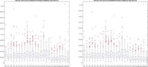
Figure 1 presents Euro dollar against US dollar exchange rate negative return hourly maxima boxplots calculated from 1-minute returns and 5-minute returns in 24 1-hour intervals (h0 - (12:00 AM- 1:00 AM), h1 - (1:00 - 2:00 AM), …, h23 (11:00 PM - 11:59 PM)) from 01/01/2003 - 12/31/2018. Clearly, the trading behaviors in different time intervals are different. The daily maxima can fall in any of those 24 hourly intervals. As a result, the daily maxima is a mixture of hourly maxima. Motivated from this kind of observations, Cao and Zhang (2020) developed new extreme value theory for maxima of maxima.

Figure 1. Euro dollar against US dollar exchange rate hourly maxima of 1 min (left panel) and 5 min (right panel) negative returns. The x-tickers are (h0 - (12:00 AM- 1:00 AM), h1 - (1:00 - 2:00 AM), …, h23 (11:00 PM - 11:59 PM) from left to right, respectively.

Suppose that the mixed sequence $\{X_i{\}}_{i=1}^n$ is composed of k subsequences $\{X_{j,i}{\}}_{i=1}^{n_j},j=1,2,\dots ,k$, $n_j\to \mathrm{\infty }$ as $n\to \mathrm{\infty }$ and $n=n_1+\cdots +n_k$. Denote $M_{j,n_j}=max(X_{j,i},i=1,\dots ,n_j)$ as the maximum of each subsequence, $\left\{X_{j,i}{\}}_{i=1}^{n_j}\stackrel{i.i.d.}{\sim }{F}_j\right(x),j=1,2,\dots ,k$. Suppose $F_j\in MDA\left(H_j\right)$, i.e., $M_{j,n_j}$ has the following limit distribution with some norming constants $a_{j,n_j}>0,b_{j,n_j}\in \mathbb{R}$, (23) $\begin{array}{r}\underset{n\to \mathrm{\infty }}{lim}P\left(a_{j,n_j}^{-1}\right(M_{j,n_j}-b_{j,n_j})\le x)=H_j\left(x\right).\end{array}$(23) Define $M_n=max(M_{1,n_1},M_{2,n_2},\dots ,M_{k,n_k})$. Questions can be asked: (1) whether or not (3(3) $\begin{array}{rl}\underset{n\to \mathrm{\infty }}{lim}{F}^n(a_{n}x+b_n)& =\underset{n\to \mathrm{\infty }}{lim}P\left(\frac{M_n-b_n}{a_n}\le x\right)\\ & =H\left(x\right)\end{array}$(3) ) holds with appropriately chosen norming constants $a_n>0,b_n\in \mathbb{R}$; (2) if (1) holds, whether or not $a_n>0,b_n\in \mathbb{R}$ are equivalent to any of $a_{j,n_j}>0,b_{j,n_j}\in \mathbb{R}$; (3) whether or not $H\left(x\right)$ is a function of $H_j\left(x\right)$; (4) if all (1)–(3) hold, which one is the best method to be used in practice. We include some new results from Cao and Zhang (2020) in the next.

Theorem 3.9

If $M_{1,n_1}$ and $M_{2,n_2}$ satisfy (23(23) $\begin{array}{r}\underset{n\to \mathrm{\infty }}{lim}P\left(a_{j,n_j}^{-1}\right(M_{j,n_j}-b_{j,n_j})\le x)=H_j\left(x\right).\end{array}$(23) ) for j = 1, 2, the limit distribution of $M_n$ as $n\to \mathrm{\infty }$ can be determined in the following cases:

• Case 1. If $\frac{a_{2,n_1}}{a_{1,n_2}}\to a>0$, $a_{1,n_1}^{-1}(b_{2,n_2}-b_{1,n_1})\to b<+\mathrm{\infty }$, for some constants a and b, then (24) $\begin{array}{r}P\left(a_{2,n_2}^{-1}\right(M_n-b_{2,n_2})\le x)\to H_1(ax+b)H_2\left(x\right).\end{array}$(24)

• Case 2. If $\frac{a_{2,n_1}}{a_{1,n_2}}\to 0$, $a_{1,n_1}^{-1}(b_{2,n_2}-b_{1,n_1})\to +\mathrm{\infty }$ then (25) $\begin{array}{r}P\left(a_{2,n_2}^{-1}\right(M_n-b_{2,n_2})\le x)\to H_2\left(x\right).\end{array}$(25)

Definition 3.10

For the independent sequence $\{X_i{\}}_{i=1}^n$ with two subsequences $\{X_{1,i}{\}}_{i=1}^{n_1}$ and $\{X_{2,i}{\}}_{i=2}^{n_2}$ defined as above, suppose (23(23) $\begin{array}{r}\underset{n\to \mathrm{\infty }}{lim}P\left(a_{j,n_j}^{-1}\right(M_{j,n_j}-b_{j,n_j})\le x)=H_j\left(x\right).\end{array}$(23) ) is satisfied with j = 1, 2 and norming constants $a_{j,n_j}>0,b_{j,n_j}\in \mathbb{R}$, i.e., (26) $\begin{array}{r}\underset{n\to \mathrm{\infty }}{lim}P\left(a_{j,n_j}^{-1}\right(M_{j,n_j}-b_{j,n})\le x)=H_j\left(x\right),j=1,2,\end{array}$(26) and (27) $\begin{array}{rl}& P\left(a_{1,n_1}^{-1}\right(M_{1,n_1}-b_{1,n_1})\le x,a_{2,n_2}^{-1}(M_{2,n_2}-b_{2,n_2})\le x)\\ & \to H\left(x\right)=H_1\left(x\right)H_2\left(x\right).\end{array}$(27) Then we call $H\left(x\right)=H_1\left(x\right)H_2\left(x\right)$ the accelerated max-stable distribution, which is the product of two max-stable distributions.

Since $H_1\left(x\right)$ and $H_2\left(x\right)$ are max-stable distributions, for any $n_1=2,3,\dots$ and $n_2=2,3,\dots$, there are constants $a_{1,n_1}>0$, $b_{1,n_1}\in \mathbb{R}$, $a_{2,n_2}>0$, $b_{2,n_2}\in \mathbb{R}$ such that $H_1\left(x\right)H_2\left(x\right)=H_1^{n_1}(a_{1,n}x+b_{1,n})H_2^{n_2}(a_{2,n}x+b_{2,n})$.

In equation (27(27) $\begin{array}{rl}& P\left(a_{1,n_1}^{-1}\right(M_{1,n_1}-b_{1,n_1})\le x,a_{2,n_2}^{-1}(M_{2,n_2}-b_{2,n_2})\le x)\\ & \to H\left(x\right)=H_1\left(x\right)H_2\left(x\right).\end{array}$(27) ), we considered the convergence of $P(max(a_{1,n_1}^{-1}(M_{1,n_1}-b_{1,n_1}),a_{2,n_2}^{-1}(M_{2,n_2}-b_{2,n_2}))\le x),$instead of the traditional $P\left(a_n^{-1}\right(M_n-b_n)\le x)$. If $n_1$ and $n_2$ are sufficiently large, by (26(26) $\begin{array}{r}\underset{n\to \mathrm{\infty }}{lim}P\left(a_{j,n_j}^{-1}\right(M_{j,n_j}-b_{j,n})\le x)=H_j\left(x\right),j=1,2,\end{array}$(26) ) we have $P\left(a_{1,n_1}^{-1}\right(M_{1,n_1}-b_{1,n_1})\le x)\approx G_1\left(x\right)$ and $P\left(a_{2,n_2}^{-1}\right(M_{2,n_2}-b_{2,n_2})\le x)\approx G_2\left(x\right)$, then (28) $\begin{array}{rl}P(M_n\le x)& =P(max(M_{1,n_1},M_{2,n_2})\le x)\\ & =P(M_{1,n_1}\le x)P(M_{2,n_2}\le x)\\ & \approx G_1(a_{1,n_1}x+b_{1,n_1})G_2(a_{2,n_2}x+b_{2,n_2})\\ & =G_1^{\ast }\left(x\right)G_2^{\ast }\left(x\right)\end{array}$(28) where $G_j^{\ast }$ is of the same type as $G_j$, j = 1, 2.

Theorem 3.11

Suppose $\{X_i{\}}_{i=1}^n$ is an independent sequence which is mixed with two subsequences $\{X_{1,i}{\}}_{i=1}^{n_1}$ and $\{X_{2,i}{\}}_{i=1}^{n_2}$ with underlying distributions $F_1\left(x\right)$ and $F_2\left(x\right)$, $n_1\to \mathrm{\infty }$ and $n_2\to \mathrm{\infty }$ as $n\to \mathrm{\infty }$. Let $0\le \tau <\mathrm{\infty }$ and $\{u_{1,i}{\}}_{i=1}^{n_1}$ and $\{u_{2,i}{\}}_{i=1}^{n_2}$ are two sequences of real numbers such that (29) $\begin{array}{rl}& n_1(1-F_1(u_{1,n_1}\left)\right)+n_2(1-F_2(u_{2,n_2}\left)\right)\to \tau \\ & \text{as }n\to \mathrm{\infty }.\end{array}$(29) Then (30) $\begin{array}{r}P(M_{1,n_1}\le u_{1,n_1},M_{2,n_2}\le u_{2,n_2})\to e^{-\tau }\text{as }n\to \mathrm{\infty }.\end{array}$(30) Conversely, if (30(30) $\begin{array}{r}P(M_{1,n_1}\le u_{1,n_1},M_{2,n_2}\le u_{2,n_2})\to e^{-\tau }\text{as }n\to \mathrm{\infty }.\end{array}$(30) ) holds for some $0\le \tau <\mathrm{\infty }$, then so does (29(29) $\begin{array}{rl}& n_1(1-F_1(u_{1,n_1}\left)\right)+n_2(1-F_2(u_{2,n_2}\left)\right)\to \tau \\ & \text{as }n\to \mathrm{\infty }.\end{array}$(29) ).

Remark 3.3

Since $1-F\left(u_{j,n_j}\right)$ is the probability that $X_{j,i}$ exceeds level $u_{j,n_j}$, equation (29(29) $\begin{array}{rl}& n_1(1-F_1(u_{1,n_1}\left)\right)+n_2(1-F_2(u_{2,n_2}\left)\right)\to \tau \\ & \text{as }n\to \mathrm{\infty }.\end{array}$(29) ) means that the expected number of exceedances of $u_{1,n_1}$ by $\{X_{1,i}{\}}_{i=1}^{n_1}$ and $u_{2,n_2}$ by $\{X_{2,i}{\}}_{i=1}^{n_2}$ in total converges to τ. When the sequence is generated from one distribution $F\left(x\right)$, Theorem 3.11 can be reduced to the classical result by choosing $u_{1,n_1}=u_{2,n_2}=u_n$. That is (31) $\begin{array}{r}n(1-F(u_n\left)\right)\to \tau ,\end{array}$(31) if and only if (32) $\begin{array}{r}P(M_n\le u_n)\to e^{-\tau }.\end{array}$(32) as $n\to \mathrm{\infty }$.

These new developments together with those in Cao and Zhang (2020) shed the light of new researches in extreme values from heterogeneous populations. They provide the probability foundation to models introduced in the next section.

4. Transforming ARMA models to models for extreme value observations

The additive structures in traditional time series models, e.g., ARMA models, and their extensions, e.g., GARCH models, cannot describe the extremal clusters and tail dependence satisfactorily in many applications. To solve this issue, alternative models have been proposed in the extreme value literature. These models transform the additive structures in ARMA models to the competing structures in extreme observations (hidden and/or observable). Several such transformations are discussed in the following subsections.

4.1. Moving minimum corresponding process

Deheuvels (1983) defined what he called the moving minimum (MM) corresponding process as $T_i=min\{{\delta }_k{Z}_{i-k},-\mathrm{\infty }<k<\mathrm{\infty }\},-\mathrm{\infty }<i<\mathrm{\infty },$where ${\delta }_k>0$, and $\left\{Z_k\right\}$ are i.i.d. standard exponential random variables. The main theorem of Deheuvels (1983) is exactly stated as the following theorem.

Theorem 4.1

If $(T_0,\dots ,T_m)$ follows a joint multivariate extreme value distribution for minima with standard exponentially distributed marginal random variables, then there exist m + 1 sequences $\left\{a_k^i\right(n),-\mathrm{\infty }<k<\mathrm{\infty }\}$ depending on $n=1,2,\dots ,$ of positive numbers, such that, if $T_i\left(n\right)=min\left\{a_k^i\right(n)Z_{-k},-\mathrm{\infty }<k<\mathrm{\infty }\}$, $i=0,\dots ,m$, then $\left(T_0\right(n),\dots ,T_m(n\left)\right)$ converges in distribution to $(T_0,\dots ,T_m)$ as $n\to \mathrm{\infty }$.

The results of Deheuvels (1983) are very strong, but the model itself is still not easily tractable for the estimation of parameters. Notice that the reciprocal of $T_i$ gives the moving maximum processes as $\begin{array}{rl}\frac{1}{T_i}& =max\left\{\frac{1}{{\delta }_k}{Z}_{i-k}^{\prime },-\mathrm{\infty }<k<\mathrm{\infty }\right\},\\ & -\mathrm{\infty }<i<\mathrm{\infty }\end{array}$where $\left\{Z_k^{\prime }\right\}$ are i.i.d. unit Fréchet random variables.

4.2. Max-autoregressive moving average process

Davis and Resnick (1989) studied what they called the max-autoregressive moving average (MARMA$(p,q)$) process of a stationary process $\left\{X_n\right\}$ which satisfies the MARMA recursion, $\begin{array}{rl}{X}_n& =\left({\varphi }_1{X}_{n-1}\right)\vee \cdots \vee \left({\varphi }_p{X}_{n-p}\right)\vee \left(Z_n\right)\\ & \vee \left({\theta }_1{Z}_{n-1}\right)\vee \cdots \vee \left({\theta }_q{Z}_{n-q}\right)\end{array}$for all n, where ∨ is a maximum operator, i.e., $a\vee b=max(a,b)$, ${\varphi }_i,{\theta }_j\ge 0,1\le i\le p,1\le j\le q$ and $\left\{Z_n\right\}$ is i.i.d. with common distribution function $F\left(x\right)=\exp \{-\sigma x^{-1}\}$. For any given $\left\{{\varphi }_i\right\},\left\{{\theta }_j\right\}$, the corresponding process is a max-stable process. They have argued “it is unlikely that another subclass of the max-stable processes can be found which is as broad and tractable as the MARMA class”. Some basic properties of the MARMA processes have been shown and the prediction of a max-stable process has been studied relatively completely. However, much less is known about estimation of MARMA process. For prediction, see also Davis and Resnick (1993). A naive estimation procedure for ${\varphi }_i,{\theta }_j$'s when the order q = 1 is given in Davis and Resnick (1989).

4.3. Multivariate maxima of moving maxima process

Smith and Weissman (1996) extended Deheuvels' MM process to a more general framework which is called multivariate maxima of moving maxima (henceforth M4) process. The definition is (33) $\begin{array}{r}{Y}_{id}=\underset{l}{max}\underset{k}{max}{a}_{l,k,d}{Z}_{l,i-k},d=1,\dots ,D,\end{array}$(33) where $\{Z_{li},l\ge 1,-\mathrm{\infty }<i<\mathrm{\infty }\}$ are an array of independent unit Fréchet random variables. The constants $\{a_{l,k,d},l\ge 1,-\mathrm{\infty }<k<\mathrm{\infty },1\le d\le D\}$ are nonnegative constants satisfying (34) $\begin{array}{r}\sum _{l=1}^{\mathrm{\infty }}\sum _{k=-\mathrm{\infty }}^{\mathrm{\infty }}{a}_{l,k,d}=1\text{for }d=1,\dots ,D.\end{array}$(34) As we see that M4 processes deal with D dimensional random processes whereas MM processes deal with univariate processes (D = 1). Under the model (33(33) $\begin{array}{r}{Y}_{id}=\underset{l}{max}\underset{k}{max}{a}_{l,k,d}{Z}_{l,i-k},d=1,\dots ,D,\end{array}$(33) ), Smith and Weissman (1996) have shown very attractive results. Some are parallel to the results of Deheuvels (1983). Although MM processes are only specified over one index there are possibilities to easily extend to over two indexes. The extension of MM processes to M4 processes results in hopes to estimate model parameters easily. Following de Haan (1984), (33(33) $\begin{array}{r}{Y}_{id}=\underset{l}{max}\underset{k}{max}{a}_{l,k,d}{Z}_{l,i-k},d=1,\dots ,D,\end{array}$(33) ) defines max-stable processes because for any finite number r and positive constants $\left\{y_{id}\right\}$ we have (35) $\begin{array}{rl}& P(Y_{id}\le y_{id},1\le i\le r,1\le d\le D)\\ & =P\left(Z_{l,i-k}\le \frac{y_{id}}{a_{l,k,d}}\text{ for }l\ge 1,-\mathrm{\infty }<k<\mathrm{\infty },\right.\\ & \left.\phantom{\frac{y_{id}}{a_{l,k,d}}}1\le i\le r,1\le d\le D\right)\\ & =P\left(Z_{l,m}\le \underset{1-m\le k\le r-m}{min}\underset{1\le d\le D}{min}\frac{y_{m+k,d}}{a_{l,k,d}},l\ge 1,\right.\\ & \left.\phantom{\frac{y_{id}}{a_{l,k,d}}}-\mathrm{\infty }<m<\mathrm{\infty }\right)\\ & =\exp \left(-\sum _{l=1}^{\mathrm{\infty }}\sum _{m=-\mathrm{\infty }}^{\mathrm{\infty }}\underset{1-m\le k\le r-m}{max}\underset{1\le d\le D}{max}\frac{a_{l,k,d}}{y_{m+k,d}}\right).\end{array}$(35) This is (2.5) of Smith and Weissman (1996) and we have $\begin{array}{rl}& P^n(Y_{id}\le n{y}_{id},1\le i\le r,1\le d\le D)\\ & =P(Y_{id}\le y_{id},1\le i\le r,1\le d\le D)\end{array}$which tells that $\left\{{\mathbf{Y}}_i\right\}$ are max-stable. They have argued that the extreme values of a multivariate stationary process may be characterised in terms of a limit max-stable process under quite general conditions. They also showed that a very large class of max-stable processes may be approximated by the M4 processes mainly because those processes have the same multivariate extremal index (Theorem 2.3 in Smith & Weissman, 1996). The theorem and conditions appear below.

Now fix $\tau =({\tau }_1,\dots ,{\tau }_D{)}^{\prime }$ with $0\le {\tau }_d<\mathrm{\infty },$ $d=1,\dots ,D$. Let $\{u_{nd},n\ge 1\}$ be a sequence of thresholds such that $n\{1-F_d(u_{nd}\left)\right\}\to {\tau }_d$ under the model assumption. Since $Z_{lk}$ is unit Fréchet we can take $u_{nd}=\frac{n}{{\tau }_d}$. Denote ${\mathbf{u}}_n=(u_{n1},\dots ,u_{nd})$ and ${\mathcal{B}}_j^k\left({\mathbf{u}}_n\right)$ the σ-field generated by the events $\{X_{id}\le u_{nd},j\le i\le k,1\le d\le D\}$ for $1\le j\le k\le n$. Define (36) $\begin{array}{rl}{\alpha }_{nt}& =sup\left\{|P\right(A\cap B)-P(A\left)P\right(B)|:A\in {\mathcal{B}}_1^k({\mathbf{u}}_n),\\ & B\in {\mathcal{B}}_{k+t}^n\left({\mathbf{u}}_n\right)\}\end{array}$(36) where the supremum is taken over $1\le k\le n-t$ and two respective σ-fields. If there exists a sequence $\{t_n,n\ge 1\}$ such that (37) $\begin{array}{r}{t}_n\to \mathrm{\infty },t_n/n\to 0,{\alpha }_{n,t_n}\to 0\text{as }n\to \mathrm{\infty },\end{array}$(37) the mixing condition $\mathrm{△}\left({\mathbf{u}}_n\right)$ is said to hold (Nandagopalan, 1994; Smith & Weissman, 1996). Further assuming there exists a sequence $\{k_n,n\ge 1\}$ such that (38) $\begin{array}{r}{k}_n\to \mathrm{\infty },k_n{t}_n/n\to 0,k_n{\alpha }_{n,t_n}\to 0\text{as }n\to \mathrm{\infty }.\end{array}$(38) Let $r_n=\left[n/k_n\right]$ be the integer part of $n/k_n$. We now exactly state a lemma and a theorem (Lemma 2.2 and their main theorem Theorem 2.3 of Smith & Weissman, 1996.)

Lemma 4.2

Suppose (36(36) $\begin{array}{rl}{\alpha }_{nt}& =sup\left\{|P\right(A\cap B)-P(A\left)P\right(B)|:A\in {\mathcal{B}}_1^k({\mathbf{u}}_n),\\ & B\in {\mathcal{B}}_{k+t}^n\left({\mathbf{u}}_n\right)\}\end{array}$(36) )–(38(38) $\begin{array}{r}{k}_n\to \mathrm{\infty },k_n{t}_n/n\to 0,k_n{\alpha }_{n,t_n}\to 0\text{as }n\to \mathrm{\infty }.\end{array}$(38) ) hold. Then (39) $\begin{array}{rl}\theta \left(\mathit{\tau }\right)& =\underset{n\to \mathrm{\infty }}{lim}P\left(Y_{id}\le u_{nd},2\le i\le r_n,\phantom{\left(\frac{Y_{1d}}{u_{nd}}\right)}\right.\\ & \left.1\le d\le D\left|\underset{d}{max}\left(\frac{Y_{1d}}{u_{nd}}\right)\right.>1\right).\end{array}$(39) Alternatively, if we assume (40) $\begin{array}{rl}& \underset{r\to \mathrm{\infty }}{lim}\underset{n\to \mathrm{\infty }}{lim}\sum _{i=r}^{r_n}\sum _{d=1}^{D}P\left(Y_{id}>u_{nd}\left|\underset{d}{max}\left(\frac{Y_{1d}}{u_{nd}}\right)\right.>1\right)\\ & =0,\end{array}$(40) then (39(39) $\begin{array}{rl}\theta \left(\mathit{\tau }\right)& =\underset{n\to \mathrm{\infty }}{lim}P\left(Y_{id}\le u_{nd},2\le i\le r_n,\phantom{\left(\frac{Y_{1d}}{u_{nd}}\right)}\right.\\ & \left.1\le d\le D\left|\underset{d}{max}\left(\frac{Y_{1d}}{u_{nd}}\right)\right.>1\right).\end{array}$(39) ) is equivalent to (41) $\begin{array}{rl}\theta \left(\mathit{\tau }\right)& =\underset{r\to \mathrm{\infty }}{lim}\underset{n\to \mathrm{\infty }}{lim}P\left(Y_{id}\le u_{nd},2\le i\le r,\phantom{\left(\frac{Y_{1d}}{u_{nd}}\right)}\right.\\ & \left.1\le d\le D\left|\underset{d}{max}\left(\frac{Y_{1d}}{u_{nd}}\right)\right.>1\right).\end{array}$(41)

This lemma is basically a restatement of results of O'Brien, for example O'Brien (1987).

Theorem 4.3

Suppose $\mathrm{△}\left({\mathbf{u}}_n\right)$ and (40(40) $\begin{array}{rl}& \underset{r\to \mathrm{\infty }}{lim}\underset{n\to \mathrm{\infty }}{lim}\sum _{i=r}^{r_n}\sum _{d=1}^{D}P\left(Y_{id}>u_{nd}\left|\underset{d}{max}\left(\frac{Y_{1d}}{u_{nd}}\right)\right.>1\right)\\ & =0,\end{array}$(40) ) hold for $\left\{{\mathbf{Y}}_i\right\}$, so that the multivariate extremal index ${\theta }^{\mathbf{Y}}\left(\mathit{\tau }\right)$ is given by (41(41) $\begin{array}{rl}\theta \left(\mathit{\tau }\right)& =\underset{r\to \mathrm{\infty }}{lim}\underset{n\to \mathrm{\infty }}{lim}P\left(Y_{id}\le u_{nd},2\le i\le r,\phantom{\left(\frac{Y_{1d}}{u_{nd}}\right)}\right.\\ & \left.1\le d\le D\left|\underset{d}{max}\left(\frac{Y_{1d}}{u_{nd}}\right)\right.>1\right).\end{array}$(41) ). Suppose also the same assumptions hold for $\left\{{\mathbf{X}}_i\right\}$ (with the same $t_n$, $k_n$ sequences). So the multivariate extremal index ${\theta }^{\mathbf{X}}\left(\mathit{\tau }\right)$ is also given by (41(41) $\begin{array}{rl}\theta \left(\mathit{\tau }\right)& =\underset{r\to \mathrm{\infty }}{lim}\underset{n\to \mathrm{\infty }}{lim}P\left(Y_{id}\le u_{nd},2\le i\le r,\phantom{\left(\frac{Y_{1d}}{u_{nd}}\right)}\right.\\ & \left.1\le d\le D\left|\underset{d}{max}\left(\frac{Y_{1d}}{u_{nd}}\right)\right.>1\right).\end{array}$(41) ) with $X_{id}$ replacing $Y_{id}$ everywhere. Then ${\theta }^{\mathbf{Y}}\left(\mathit{\tau }\right)={\theta }^{\mathbf{X}}\left(\mathit{\tau }\right)$.

The extremal index of the process defined by (33(33) $\begin{array}{r}{Y}_{id}=\underset{l}{max}\underset{k}{max}{a}_{l,k,d}{Z}_{l,i-k},d=1,\dots ,D,\end{array}$(33) ) is (42) $\begin{array}{r}\theta \left(\mathit{\tau }\right)=\frac{\sum _l\underset{k}{max}\underset{d}{max}{a}_{l,k,d}{\tau }_d}{\sum _l\sum _k\underset{d}{max}{a}_{l,k,d}{\tau }_d}.\end{array}$(42) However, $\theta \left(\mathit{\tau }\right)$ is not easy to obtain with observed data as one has to estimate all parameters $a_{l,k,d}$, which is not straightforward.

We see that Sections 4.1–4.3 deal with probabilistic aspects of time series models for observed extreme value processes. Although theoretical results have been obtained, the estimation of parameters in both MARMA$(p,q)$ and M4 processes are not well developed and the applications of the two processes are very limited. In the next four subsections, we discuss statistical inference and applications.

4.4. Statistical inference of moving maximum models

Hall et al. (2002) discussed moving maximum models $Y_j=sup\{a_{j-i}{Z}_i,-\mathrm{\infty }<i<\mathrm{\infty }\}$where the distribution of $Z_i$ is assumed either $F\left(z|\theta \right)=\exp (-z^{-\theta })$ or the generalised Pareto distribution $F\left(z|\theta \right)=1-(1+z{)}^{-\theta }$. Then for a finite number of parameters, they chose $(\theta ,a_{\left(m\right)})$ to minimise (43) $\begin{array}{rl}& D_m(\theta ,a_{\left(m\right)})\\ & =\int \left\{\hat{G}\left(y\right)-\prod _{i=2-m}^{k}F(min\{a_{j-i}^{-1}{y}_j,\right.\\ & {\left.\phantom{\prod _{i=2-m}^k}max(i,1)\le j\le min(i+m,k)\}|\theta )\right\}}^{2}w\left(y\right)\text{d}y,\end{array}$(43) where the integral is over $y=(y_1,\dots ,y_k)\in {\mathbb{R}}_{+}^k$ and (44) $\begin{array}{r}\hat{G}\left(y\right)=(n-k{)}^{-1}\sum _{i=1}^{n-k}{I}_{(Y_{i+j-1}\le y_j\text{for }1\le j\le k)},\end{array}$(44) and w is a nonnegative weight function. We state their main theorem as follows.

Theorem 4.4

Under conditions:

• F has support on the positive half-line, and is in the domain of attraction of a Type II extreme value distribution;

• each $a_i$ is nonnegative and, for some $ϵ\in (0,r)$, $0<\sum _i{a}_i^{r-ϵ}<\mathrm{\infty }$.

Then (45) $\begin{array}{rl}& \underset{-\mathrm{\infty }<y_1,\dots ,y_k<\mathrm{\infty }}{sup}|P(Y_1^{\ast }\le y_1,\dots ,Y_k^{\ast }\le y_k|Y_1,\dots ,Y_n)\\ & -P(Y_1\le y_1,\dots ,Y_k\le y_k)|\to 0\end{array}$(45) where $Y_j^{\ast }$ is defined by $Y_j^{\ast }=sup\{{\hat{a}}_{j-i}{Z}_i^{\ast },-\mathrm{\infty }<i<\mathrm{\infty }\},$${\hat{a}}_{j-i}$ and $\hat{\theta }$ are solutions of (4.4), and $Z_i^{\ast }$ has distribution function $F(\cdot |\hat{\theta })$. Moreover, if $m\ge C_4(\log n{)}^2$ for $C_4$ sufficiently large, the rate of convergence in (45(45) $\begin{array}{rl}& \underset{-\mathrm{\infty }<y_1,\dots ,y_k<\mathrm{\infty }}{sup}|P(Y_1^{\ast }\le y_1,\dots ,Y_k^{\ast }\le y_k|Y_1,\dots ,Y_n)\\ & -P(Y_1\le y_1,\dots ,Y_k\le y_k)|\to 0\end{array}$(45) ) is $O_p\left(n^{-\left(1/2\right)+\delta }\right)$ for all $\delta >0$.

4.5. Finite representations of M4 processes

It can be seen that models having too many parameters to be estimated and/or having a complicated framework and hence lack of interpretability are hardly applicable to real data with a finite number of observations. This section reviews finite representations of M4 processes and their applications.

A finite dimensional M4 process can be written as follows: (46) $\begin{array}{r}{Y}_{id}=\underset{1\le l\le L}{max}\underset{-K_1\le k\le K_2}{max}{a}_{l,k,d}{Z}_{l,i-k},d=1,\dots ,D,\end{array}$(46) where $\sum _{l=1}^L\sum _{k=-K_1}^{K_2}{a}_{l,k,d}=1$ for $d=1,\dots ,D$.

Under model (46(46) $\begin{array}{r}{Y}_{id}=\underset{1\le l\le L}{max}\underset{-K_1\le k\le K_2}{max}{a}_{l,k,d}{Z}_{l,i-k},d=1,\dots ,D,\end{array}$(46) ), it is possible that a big value of $Z_{lk}$ dominates all other Z values within a certain period of length $K_2+K_1+1$ and creates a moving pattern, i.e., $Y_{id}=a_{l,i-k,d}{Z}_{lk}$ for i close to k. A moving pattern is known as a signature pattern. Zhang and Smith (2004) gave a full investigation of probabilistic properties of model (46(46) $\begin{array}{r}{Y}_{id}=\underset{1\le l\le L}{max}\underset{-K_1\le k\le K_2}{max}{a}_{l,k,d}{Z}_{l,i-k},d=1,\dots ,D,\end{array}$(46) ). Zhang and Smith (2010) studied the estimation of the model, and considered the bivariate joint probabilities. A general joint probability formula of (46(46) $\begin{array}{r}{Y}_{id}=\underset{1\le l\le L}{max}\underset{-K_1\le k\le K_2}{max}{a}_{l,k,d}{Z}_{l,i-k},d=1,\dots ,D,\end{array}$(46) ) is (47) $\begin{array}{rl}& P(Y_{id}\le y_{id},1\le i\le r,1\le d\le D)\\ & =\exp \left(-\sum _{l=1}^L\sum _{m=1-K}^r\underset{1-m\le k\le r-m}{max}\underset{1\le d\le D}{max}\frac{a_{l,k,d}}{y_{m+k,d}}\right),\end{array}$(47) where $a_{l,k,d}=0$ when the triple subindex is outside the range defined in (46(46) $\begin{array}{r}{Y}_{id}=\underset{1\le l\le L}{max}\underset{-K_1\le k\le K_2}{max}{a}_{l,k,d}{Z}_{l,i-k},d=1,\dots ,D,\end{array}$(46) ). Besides this general formula, it follows immediately that $P(Y_{id}\le y)=e^{-1/y}$, which establishes that $Y_{id}$ is itself a unit Fréchet random variable, and the following two special cases are used to construct estimators: (48) $\begin{array}{rl}& P(Y_{id}\le 1,Y_{i+1,d}\le x)\\ & =\exp \left(-\sum _{l=1}^L\sum _{m=1-K}^{2}max\left(a_{l,1-m,d},\frac{a_{l,2-m,d}}{x}\right)\right)\\ & =:e^{-b_{0d}\left(x\right)},\end{array}$(48) and (49) $\begin{array}{rl}& P(Y_{id}\le 1,Y_{i{d}^{\prime }}\le x)\\ & =\exp \left(-\sum _{l=1}^L\sum _{m=1-K}^{1}max\left(a_{l,1-m,d},\frac{a_{l,1-m,d^{\prime }}}{x}\right)\right)\\ & =:e^{-b_{d{d}^{\prime }}\left(x\right)}.\end{array}$(49) It is clear that for each d, we can define new piecewise linear functions: $q_{0d}\left(x\right):=x{b}_{0d}\left(x\right)$ and $q_{d{d}^{\prime }}\left(x\right):=x{b}_{d{d}^{\prime }}\left(x\right)$, where the notation A: = B means that A is denoted as B, and the points where these piecewise linear functions change slopes are at $a_{l,j,d}/a_{l,j^{\prime },d}$ or $a_{l,k,d}/a_{l,k,d^{\prime }}$. This suggests that if we can identify the functions $q_{0d}\left(x\right)$ or $q_{d{d}^{\prime }}\left(x\right)$, we may be able to identify all the parameters $a_{l,k,d}$.

Relating (48(48) $\begin{array}{rl}& P(Y_{id}\le 1,Y_{i+1,d}\le x)\\ & =\exp \left(-\sum _{l=1}^L\sum _{m=1-K}^{2}max\left(a_{l,1-m,d},\frac{a_{l,2-m,d}}{x}\right)\right)\\ & =:e^{-b_{0d}\left(x\right)},\end{array}$(48) ) and (49(49) $\begin{array}{rl}& P(Y_{id}\le 1,Y_{i{d}^{\prime }}\le x)\\ & =\exp \left(-\sum _{l=1}^L\sum _{m=1-K}^{1}max\left(a_{l,1-m,d},\frac{a_{l,1-m,d^{\prime }}}{x}\right)\right)\\ & =:e^{-b_{d{d}^{\prime }}\left(x\right)}.\end{array}$(49) ) to their empirical distribution counterparts, Zhang and Smith (2010) solves a system of piecewise linear functions to construct parameter estimators. The consistency and asymptotic normality of the estimators are established. A financial application of value at risk (VaR) is conducted. A new extreme co-movement measure is defined as (50) $\begin{array}{r}\lambda (t,T)=\underset{\mathbf{u}\nearrow {\mathbf{x}}_F}{lim}P(\xi (t,T,\mathbf{u})\ge 2|\xi (0,t,\mathbf{u})\ge 1)\end{array}$(50) and (51) $\begin{array}{r}\xi (t,T,\mathbf{u})=\underset{t\le i\le T}{max}\sum _{d=1}^D{I}_{(Y_{id}>u_d)}.\end{array}$(51) The idea in (50(50) $\begin{array}{r}\lambda (t,T)=\underset{\mathbf{u}\nearrow {\mathbf{x}}_F}{lim}P(\xi (t,T,\mathbf{u})\ge 2|\xi (0,t,\mathbf{u})\ge 1)\end{array}$(50) ) is to estimate the maximum number of joint exceedances in the time period t to T given at least one exceedance in $(0,t)$. The case t = T = 0 and D = 2 is the usual tail dependence function in the literature (Embrechts et al., 2003). Zhang and Smith (2010) demonstrated that (50(50) $\begin{array}{r}\lambda (t,T)=\underset{\mathbf{u}\nearrow {\mathbf{x}}_F}{lim}P(\xi (t,T,\mathbf{u})\ge 2|\xi (0,t,\mathbf{u})\ge 1)\end{array}$(50) ) is a meaningful market extreme co-movement measure. The tail dependence index λ, the coefficient of tail dependence η, the lag-k tail dependence index ${\lambda }_k$, the extremal index $\theta \left(\tau \right)$, and the extreme co-movement measure $\lambda (t,T)$ can be very useful in studying market crisis and contagions.

4.6. Sparse representations of M4 processes

To increase the estimation efficiency, a common strategy in statistical inference is to reduce the model complexity, i.e., to reduce the number of parameters. Examples include the variable selections in linear regression models, and the sparsity assumption in high-dimensional covariance matrix estimation. In time series, the number of parameters in an auto-regressive model is often less than the number of parameters in a moving average model when they both are fitted to a time series. To reduce the number of unknown parameters in (46(46) $\begin{array}{r}{Y}_{id}=\underset{1\le l\le L}{max}\underset{-K_1\le k\le K_2}{max}{a}_{l,k,d}{Z}_{l,i-k},d=1,\dots ,D,\end{array}$(46) ), Zhang (2008a) considered using geometric moving patterns to study extreme sea wave movements. The number of parameters in Zhang (2008a) is much smaller than the number of parameters in the model studied by Zhang and Smith (2010). This section discusses three scenarios that further simplify model (33(33) $\begin{array}{r}{Y}_{id}=\underset{l}{max}\underset{k}{max}{a}_{l,k,d}{Z}_{l,i-k},d=1,\dots ,D,\end{array}$(33) ) or (46(46) $\begin{array}{r}{Y}_{id}=\underset{1\le l\le L}{max}\underset{-K_1\le k\le K_2}{max}{a}_{l,k,d}{Z}_{l,i-k},d=1,\dots ,D,\end{array}$(46) ) to more interpretable and workable models.

4.6.1. Markov chain MM process

In this section, we consider univariate time series model. Under model (33(33) $\begin{array}{r}{Y}_{id}=\underset{l}{max}\underset{k}{max}{a}_{l,k,d}{Z}_{l,i-k},d=1,\dots ,D,\end{array}$(33) ), we have the following lag-k tail dependence index formula (drop the index d): (52) $\begin{array}{r}{\lambda }_k=\sum _{l=1}^{\mathrm{\infty }}\sum _{m=-\mathrm{\infty }}^{\mathrm{\infty }}min(a_{l,1-m},a_{l,1+k-m}).\end{array}$(52) Obviously, as long as both $a_{l0}$ and $a_{lK}$ are non-zero, $Y_i$ and $Y_{i+K}$ are dependent, and of course tail dependent as can be seen from (52(52) $\begin{array}{r}{\lambda }_k=\sum _{l=1}^{\mathrm{\infty }}\sum _{m=-\mathrm{\infty }}^{\mathrm{\infty }}min(a_{l,1-m},a_{l,1+k-m}).\end{array}$(52) ). Zhang (2005) considered the matrix of weights $\left(a_{lk}\right)$ to have the following structure: (53) $\begin{array}{r}\left(a_{lk}\right)=\left(\begin{array}{cccccc}{a}_{00}& 0& 0& 0& \cdots & 0\\ a_{10}& a_{11}& 0& 0& \cdots & 0\\ a_{20}& 0& a_{22}& 0& \cdots & 0\\ ⋮& ⋮& ⋮& ⋮& \ddots & 0\\ a_{L0}& 0& 0& 0& \dots & a_{LL}\end{array}\right).\end{array}$(53) Now the number L corresponds to the maximal lag of tail dependencies within the sequence; the lag-k tail dependence index is characterised by the coefficients $a_{k0}$ and $a_{kk}$. The coefficient $a_{00}$ represents the proportion of the number of observations which are drawn from an independent process $\left\{Z_{0i}\right\}$. In other words, a very large value at time 0 has no future impact when the large value is generated from $\left\{Z_{0i}\right\}$. If both $a_{k0}$ and $a_{kk}$ are not zero, then a very large value at time 0 has impact at time k when the large value is generated from $\left\{Z_{ki}\right\}$. If there is strong lag-k tail dependence for each k, the value of $a_{00}$ will be small. Using the structure of (53(53) $\begin{array}{r}\left(a_{lk}\right)=\left(\begin{array}{cccccc}{a}_{00}& 0& 0& 0& \cdots & 0\\ a_{10}& a_{11}& 0& 0& \cdots & 0\\ a_{20}& 0& a_{22}& 0& \cdots & 0\\ ⋮& ⋮& ⋮& ⋮& \ddots & 0\\ a_{L0}& 0& 0& 0& \dots & a_{LL}\end{array}\right).\end{array}$(53) ), Zhang (2005) proposed three models for financial times. They are presented next.

Model 4.1

Combining MM (used to model scales) with a Markov process (used to model signs): two models for transformed negative $(-)$ returns and positive $(+)$ returns are $Y_i^{\pm }=\underset{0\le l\le L^{\pm }}{max}\underset{0\le k\le K^{\pm }}{max}{a}_{lk}^{\pm }{Z}_{l,i-k}^{\pm },-\mathrm{\infty }<i<\mathrm{\infty },$where the superscript ${}^{-}$ means that the model is for negative returns only, and ${}^{+}$ means that the model is for positive returns only. In the following, we only discuss the model for negative returns, and the model for positive returns is obtained by simply replacing ${}^{-}$ by ${}^{+}$. Constants $\left\{a_{lk}^{-}\right\}$ are nonnegative and satisfy $\sum _{l=0}^{L^{-}}\sum _{k=0}^{K^{-}}{a}_{lk}^{-}=1$. The matrix of weights is $\left(a_{lk}^{-}\right)=\left(\begin{array}{cccccc}{a}_{00}^{-}& 0& 0& 0& \cdots & 0\\ a_{10}^{-}& a_{11}^{-}& 0& 0& \cdots & 0\\ a_{20}^{-}& 0& a_{22}^{-}& 0& \cdots & 0\\ ⋮& ⋮& ⋮& ⋮& \ddots & 0\\ a_{L^{-}0}^{-}& 0& 0& 0& \dots & a_{L^{-}{L}^{-}}^{-}\end{array}\right).$$\{Z_{li}^{-},l=1,\dots ,L^{-},$ $-\mathrm{\infty }<i<\mathrm{\infty }\}$ is an independent array, where random variables $Z_{li}^{-}$ are identically unit Fréchet distributed. Let (54) $\begin{array}{r}{R}_i^{-}={\xi }_i^{-}{Y}_i^{-},-\mathrm{\infty }<i<\mathrm{\infty },\end{array}$(54) where the process $\left\{{\xi }_i^{-}\right\}$ is independent of $\left\{Y_i^{-}\right\}$ and takes values in a finite set {0, 1} – i.e., $\left\{{\xi }_i^{-}\right\}$ is a sign process. Here $\left\{Y_i^{-}\right\}$ is an MM process, $\left\{{\xi }_i^{-}\right\}$ is a simple Markov process. $\left\{R_i^{-}\right\}$ is the negative return process. For simplicity, Model (54(54) $\begin{array}{r}{R}_i^{-}={\xi }_i^{-}{Y}_i^{-},-\mathrm{\infty }<i<\mathrm{\infty },\end{array}$(54) ) is regarded as MCMM processes.

Remark 4.1

If $\left\{Y_i^{-}\right\}$ is an independent process, then $P(R_{i+r}^{-}>u|R_i^{-}>u)\to 0$ as $u\to \mathrm{\infty }$ for i>0, r>0, i.e., no tail dependence exists. This phenomenon tells that if there are tail dependencies in the observed process, the model with time dependence (through a Markov chain) only can not model the tail dependence if the random variables used to model scales are not tail dependent.

Remark 4.2

Empirical studies show that negative returns $Y_i^{-}$ and positive returns $Y_i^{+}$ are asymmetric, and conclude that models for positive returns should be different from models for negative returns. Notice that at any time i, one can only observe one of the $Y_i^{-}$ and $Y_i^{+}$. The other one is missing. By introducing the Markov processes ${\xi }_i^{-}$ and ${\xi }_i^{+}$, both $R_i^{-}$ and $R_i^{+}$ in (54(54) $\begin{array}{r}{R}_i^{-}={\xi }_i^{-}{Y}_i^{-},-\mathrm{\infty }<i<\mathrm{\infty },\end{array}$(54) ) are observable. We use $R_i^{-}$ and $R_i^{+}$ to construct parameter estimators.

Model 4.2

An MCMM process model for returns: with the established notations in (54(54) $\begin{array}{r}{R}_i^{-}={\xi }_i^{-}{Y}_i^{-},-\mathrm{\infty }<i<\mathrm{\infty },\end{array}$(54) ), let (55) $\begin{array}{rl}{R}_i& =\text{sign}\left({\xi }_i\right)\ast [I_{{\xi }_i=-1}{Y}_i^{-}+I_{{\xi }_i=1}{Y}_i^{+}],\\ & -\mathrm{\infty }<i<\mathrm{\infty },\end{array}$(55) where the process $\left\{{\xi }_i\right\}$ is a simple Markov process which is independent of $\left\{Y_i^{\pm }\right\}$ and takes values in a finite set $\{-1,0,1\}$. $\left\{R_i\right\}$ is the return process.

Remark 4.3

The processes $\left\{{\xi }_i^{-}\right\}$, $\left\{{\xi }_i^{+}\right\}$ may be Bernoulli processes or Markov processes taking values in a finite set. The process $\left\{{\xi }_i\right\}$ may be considered as an independent process or a Markov process taking values in a finite set.

Remark 4.4

In Model (55(55) $\begin{array}{rl}{R}_i& =\text{sign}\left({\xi }_i\right)\ast [I_{{\xi }_i=-1}{Y}_i^{-}+I_{{\xi }_i=1}{Y}_i^{+}],\\ & -\mathrm{\infty }<i<\mathrm{\infty },\end{array}$(55) ), as long as $Y_i^{-}$, $Y_i^{+}$, and ${\xi }_i$ are determined, $R_i$ is determined.

Remark 4.5

In many applications, only positive observed values are concerned. Insurance claims, annual maxima of precipitations, file sizes, durations in internet traffic at a certain point are some of those examples having positive values only. Even in our negative return model, the values have been converted into positive values.

4.6.2. Sparse random coefficient M4 processes

One feature in M4 processes is its signature patterns. To fit the data better, we may need a large number of patterns. One way to get rid of this feature is to set moving coefficients to be random. Tang et al. (2013) considered a sparse M4 random coefficient model (SM4R), which has a parsimonious number of parameters, and it can potentially capture the major stylised facts exhibited by devolatised financial time series found in empirical studies. They demonstrated through real data analysis that the SM4R model can effectively be used to improve the estimates of the value at risk for portfolios consisting of multivariate financial returns while ignoring either temporal or cross-sectional tail dependence could potentially result in a serious underestimate of market risk.

The SM4R model is defined as (56) $\begin{array}{rl}{X}_{td}& =max[{\mathbf{B}}_d^{\left(t\right)}\cdot {\mathbf{Z}}_d^{\left(t\right)}],\\ & d=1,\dots ,D,-\mathrm{\infty }<t<\mathrm{\infty },\end{array}$(56) $\begin{array}{rl}& {\mathbf{B}}_d^{\left(t\right)}=\left(\begin{array}{ccccc}{\text{β}}_{00d}^{\left(t\right)}& 0& 0& \cdots & 0\\ {\text{β}}_{10d}^{\left(t\right)}& {\text{β}}_{11d}^{\left(t\right)}& 0& \cdots & 0\\ {\text{β}}_{20d}^{\left(t\right)}& 0& {\text{β}}_{22d}^{\left(t\right)}& \cdots & 0\\ ⋮& ⋮& ⋮& \ddots & ⋮\\ {\text{β}}_{L_{d}0d}^{\left(t\right)}& 0& 0& \cdots & {\text{β}}_{L_d{L}_{d}d}^{\left(t\right)}\end{array}\right),\\ & {\mathbf{Z}}_d^{\left(t\right)}=\left(\begin{array}{cccc}{Z}_{0td}& Z_{0,t-1,d}& \cdots & Z_{0,t-L_d,d}\\ Z_{1td}& Z_{1,t-1,d}& \cdots & Z_{1,t-L_d,d}\\ ⋮& ⋮& \ddots & ⋮\\ Z_{L_{d}td}& Z_{L_d,t-1,d}& \cdots & Z_{L_d,t-L_d,d}\end{array}\right),\end{array}$where $\{{\mathbf{Z}}_{0t}=(Z_{0t1},\dots ,Z_{0tD}\left)\right\}$ is a sequence of i.i.d. D-dimensional random vectors (across t) having a multivariate extreme value distribution function with unit Fréchet margins, $\left\{Z_{ltd}\right\}$ are i.i.d. unit Fréchet random variables for $l\ge 1$, ${\text{β}}_{00d}^{\left(t\right)}=b_{0d}$, ${\text{β}}_{l0d}^{\left(t\right)}=a_{ltd}{b}_{ld}$ and ${\text{β}}_{lld}^{\left(t\right)}=(1-a_{ltd})b_{ld}$, $l=1,\dots ,L_d$, $d=1,\dots ,D$, $\left\{a_{ltd}\right\}$ are i.i.d. random variables on interval $[0,1]$, $\mathbf{b}=\{b_{ld},l=1,\dots ,L_d,d=1,\dots ,D\}$ are positive constants with $\sum _{l=0}^{L_d}{b}_{ld}=1$ for any d, and $\left\{{\mathbf{Z}}_{0t}\right\}$, $\left\{a_{ltd}\right\}$, and $\{Z_{ltd}:l\ge 1\}$ are independent with each other.

The cross-sectional tail dependence at time t is characterised by the copula function of ${\mathbf{Z}}_{0t}$ and tuned by $\{b_{0d},d=1,\dots ,D\}$. With this setup, all kinds of parametric multivariate extreme value distributions can naturally be incorporated into the SM4R structure so that a parsimonious model with satisfactory level of generality can be achieved. This contrasts with the classical M4 setting where all components depend on the same set of shock variables $Z_{lt}$, which inherently restricts the dependence structure to a given type and often requires a large number of parameters to achieve satisfactory performance.

For any $t=1,\dots ,r$ and positive constants $\mathbf{x}=\{x_{td},t=1,\dots ,r,d=1,\dots ,D\}$, the joint distribution function of $\{X_{td},t=1,\dots ,r,d=1,\dots ,D\}$ conditional on the generic random vector $\mathbf{a}$ representing all the $a_{lkd}$'s involved is (57) $\begin{array}{rl}& P(X_{td}\le x_{td},1\le t\le r,1\le d\le D|\mathbf{a})\\ & =\exp \{-V(\mathbf{x},\mathbf{a};\mathbf{b}\left)\right\},\end{array}$(57) where $V(\mathbf{x},\mathbf{a};\mathbf{b})$ is defined as $\begin{array}{rl}V(\mathbf{x},\mathbf{a};\mathbf{b})& =\sum _{t=1}^r{V}_{\ast }\left(\frac{x_{t1}}{b_{01}},\dots ,\frac{x_{tD}}{b_{0D}}\right)\\ & +\sum _{d=1}^D\sum _{l=1}^L{b}_{ld}\left[\sum _{j=1}^{min(l,r)}\frac{1-a_{ljd}}{x_{jd}}\right.\\ & +\sum _{j^{\mathrm{\prime }}=1}^{max(r-l,0)}max\left(\frac{a_{l{j}^{\mathrm{\prime }}d}}{x_{j^{\mathrm{\prime }}d}},\frac{1-a_{l,j^{\mathrm{\prime }}+l,d}}{x_{j^{\mathrm{\prime }}+l,d}}\right)\\ & \left.+\sum _{j^{\mathrm{\prime }\mathrm{\prime }}=max(r-l,0)+1}^r\frac{a_{l{j}^{\mathrm{\prime }\mathrm{\prime }}d}}{x_{j^{\mathrm{\prime }\mathrm{\prime }}d}}\right],\end{array}$$\exp (-V_{\ast }(\cdot \left)\right)=\exp (-V_{\ast }(\cdot |{\theta }_{Z_0}\left)\right)$ is the multivariate extreme value distribution of ${\mathbf{Z}}_{0t}$, and $V_{\ast }(\cdot )$ is called the exponent measure of ${\mathbf{Z}}_{0t}$ (e.g., Resnick, 1987). A proof of (57(57) $\begin{array}{rl}& P(X_{td}\le x_{td},1\le t\le r,1\le d\le D|\mathbf{a})\\ & =\exp \{-V(\mathbf{x},\mathbf{a};\mathbf{b}\left)\right\},\end{array}$(57) ) can be found in Tang et al. (2013). The marginal distribution of $X_{td}$ is still unit Fréchet and the multivariate distribution function of $(X_{t1},\dots ,X_{tD})$ is (58) $\begin{array}{rl}& P(X_{td}\le x_{td},1\le d\le D)\\ & =\exp \left\{-\sum _{d=1}^D\frac{1}{x_{td}}(1-b_{0d})-V_{\ast }\left(\frac{x_{t1}}{b_{01}},\dots ,\frac{x_{tD}}{b_{0D}}\right)\right\},\end{array}$(58) a new multivariate extreme value distribution function whose dependence is characterised by a mixture of independent and extreme value copulas.

One of the most popular multivariate extreme value distributions in practice is the logistic distribution (Gumbel-Hougaard copula with unit Fréchet margins) defined as: (59) $\begin{array}{r}{G}_{\log }(\mathbf{x};\alpha )=\exp \left\{-{\left(\sum _{d=1}^D{x}_d^{-1/\alpha }\right)}^{\alpha }\right\},\end{array}$(59) where $\alpha \in (0,1]$. When ${\mathbf{Z}}_{0t}\sim G_{\log }(\cdot ;\alpha )$, the joint distribution function (58(58) $\begin{array}{rl}& P(X_{td}\le x_{td},1\le d\le D)\\ & =\exp \left\{-\sum _{d=1}^D\frac{1}{x_{td}}(1-b_{0d})-V_{\ast }\left(\frac{x_{t1}}{b_{01}},\dots ,\frac{x_{tD}}{b_{0D}}\right)\right\},\end{array}$(58) ) becomes (60) $\begin{array}{rl}& P(X_{td}\le x_{td},1\le d\le D)\\ & =\exp \left\{-\sum _{d=1}^D\frac{1}{x_{td}}(1-b_{0d})-{\left[\sum _{d=1}^D{\left(\frac{b_{0d}}{x_{td}}\right)}^{\frac{1}{\alpha }}\right]}^{\alpha }\right\}.\end{array}$(60) When D = 2, the cross-sectional bivariate distribution defined by (60(60) $\begin{array}{rl}& P(X_{td}\le x_{td},1\le d\le D)\\ & =\exp \left\{-\sum _{d=1}^D\frac{1}{x_{td}}(1-b_{0d})-{\left[\sum _{d=1}^D{\left(\frac{b_{0d}}{x_{td}}\right)}^{\frac{1}{\alpha }}\right]}^{\alpha }\right\}.\end{array}$(60) ) is just the asymmetric logistic distribution proposed by Tawn (1988). Interestingly, the copula function of (60(60) $\begin{array}{rl}& P(X_{td}\le x_{td},1\le d\le D)\\ & =\exp \left\{-\sum _{d=1}^D\frac{1}{x_{td}}(1-b_{0d})-{\left[\sum _{d=1}^D{\left(\frac{b_{0d}}{x_{td}}\right)}^{\frac{1}{\alpha }}\right]}^{\alpha }\right\}.\end{array}$(60) ) is $\begin{array}{rl}C(u_1,\dots ,u_D)& =C_{\log }(u_1^{b_{01}},\dots ,u_D^{b_{0D}})\\ & \times C_{\perp }(u_1^{1-b_{01}},\dots ,u_D^{1-b_{0D}}),\end{array}$where $C_{\log }$ and $C_{\perp }$ are the Gumbel-Hougaard copula and independent copula, respectively. In general, if $\{C_j,j=1,\dots ,P\}$ are P D-dimensional copulas and $\left\{b_{jd}\right\}$ are any positive constants satisfying $\sum _{j=1}^P{b}_{jd}=1$ for $d=1,\dots ,D$, then the function $C^{\ast }$ constructed as $C^{\ast }(u_1,\dots ,u_D)=\prod _{j=1}^P{C}_j(u_1^{b_{j1}},\dots ,u_D^{b_{jD}})$ is still a copula function associated with a D-dimensional distribution function. To see this, consider the process $\left\{Y_{td}\right\}$ defined as $Y_{td}=\underset{1\le j\le P}{max}{b}_{jd}{Z}_{tjd}$ for $d=1,\dots ,D$, where $\left\{\right(Z_{tj1},\dots ,Z_{tjD}),j=1,\dots ,P,t=1,\dots ,\}$ are i.i.d. D-variate random vectors with copula $C_j$ and unit Fréchet margins. It can be checked that $C^{\ast }$ is the copula of $(Y_{t1},\dots ,Y_{tD})$.

Besides the above discussed properties of model (56(56) $\begin{array}{rl}{X}_{td}& =max[{\mathbf{B}}_d^{\left(t\right)}\cdot {\mathbf{Z}}_d^{\left(t\right)}],\\ & d=1,\dots ,D,-\mathrm{\infty }<t<\mathrm{\infty },\end{array}$(56) ), there are many other related properties and developments of the model can be found in Tang et al. (2013). The estimators for the model parameters are constructed using GMM approach. We refer the details to Tang et al. (2013).

4.6.3. Copula structured M4 processes

Statistical applications of classical parametric max-stable processes are still sparse mostly due to lack of (1) efficiency of statistical estimation of many parameters in the processes, (2) flexibility of concurrently modeling asymptotic independence, and asymptotic dependence among variables, and (3) capability of fitting real data directly. Zhang and Zhu (2016) studied a more flexible model, i.e., a class of copula structured M4 (multivariate maxima and moving maxima) processes, and hence CSM4 for short. CSM4 processes are constructed by incorporating sparse random coefficients and structured extreme value copulas in asymptotically (in)dependent M4 (AIM4) processes. It is shown that the new model overcomes all of the aforementioned three constraints. They illustrated new features and advantages of the CSM4 model using simulated examples and real data of intra-daily maxima of high-frequency financial time series. They also studied the probabilistic properties of the proposed model and its statistical inference.

In Zhang and Zhu (2016), they first proposed a new model that is good for marginally transformed observations. It is defined as: (61) $\begin{array}{rl}{Y}_{td}& =max(W_{td}^{1/{\text{β}}_d},max[{\mathbf{A}}_{td}\cdot {\mathbf{Z}}_t]),\\ & d=1,\dots ,D,-\mathrm{\infty }<t<\mathrm{\infty },\end{array}$(61) where ${\text{β}}_d>0,d=1,\dots ,D$; $\{W_t,\mathrm{\infty }<t<\mathrm{\infty }\}=\left\{\right(W_{t1},\dots ,W_{tD}),\mathrm{\infty }<t<\mathrm{\infty }\}$ is a sequence of i.i.d. D-dimensional random vectors following logistic distribution defined the same as (59(59) $\begin{array}{r}{G}_{\log }(\mathbf{x};\alpha )=\exp \left\{-{\left(\sum _{d=1}^D{x}_d^{-1/\alpha }\right)}^{\alpha }\right\},\end{array}$(59) ) with $\mathbf{x}=(x_1,\dots ,x_D)$ and $\gamma =1/\alpha \ge 1$. ${\mathbf{A}}_{td}$ is a sparse random loading matrix having the form: $\begin{array}{rl}{\mathbf{A}}_{td}& =\left(\begin{array}{ccc}{\alpha }_{1d}{U}_{1td}& {\alpha }_{1d}(1-U_{1td})& 0\\ {\alpha }_{2d}{U}_{2td}& 0& {\alpha }_{2d}(1-U_{2td})\\ ⋮& ⋮& ⋮\\ {\alpha }_{Ld}{U}_{Ltd}& 0& 0\end{array}\right.\\ & \left.\begin{array}{cc}\cdots & 0\\ \cdots & 0\\ \ddots & ⋮\\ \cdots & {\alpha }_{Ld}(1-U_{Ltd})\end{array}\right)\end{array}$with ${\alpha }_{ld}\ge 0$, $\sum _{l=1}^L{\alpha }_{ld}=1$ for each d, and $\{U_{ltd},1=1,\dots ,L,-\mathrm{\infty }<t<\mathrm{\infty },d=1,\dots ,D\}$ being i.i.d. nondegenerated random variables on $[0,1]$. For $-\mathrm{\infty }<t<\mathrm{\infty }$, $Z_t=\left\{\right(Z_{l,t-j+1}),1=1,\dots ,L;j=1,\dots ,L+1\}$ is an independent array, with $Z_{l,t-j}$'s being unit Fréchet random variables; ${\mathbf{A}}_{td}\cdot {\mathbf{Z}}_t$ represents the componentwise products between matrices ${\mathbf{A}}_{td}$ and ${\mathbf{Z}}_t$ at time t, and $\{max\mathbf{C}\}$ takes the maximum over all elements of matrix $\mathbf{C}$. $\left\{Z_{lt}\right\}$, $\left\{U_{ltd}\right\}$ and $\left\{{\mathbf{W}}_{\mathbf{t}}\right\}$ are assumed to be independent of each other.

In the second step, assuming that $\{{\mathbf{X}}_t=(X_{t1},\dots ,X_{tD}),t=1,2,\dots \}$ is an observable multivariate stationary time series, they generalised (61(61) $\begin{array}{rl}{Y}_{td}& =max(W_{td}^{1/{\text{β}}_d},max[{\mathbf{A}}_{td}\cdot {\mathbf{Z}}_t]),\\ & d=1,\dots ,D,-\mathrm{\infty }<t<\mathrm{\infty },\end{array}$(61) ) to a directly applicable model: (62) $\begin{array}{r}{X}_{td}=C_d{Y}_{td}^{1/{\psi }_d},d=1,\dots ,D,\end{array}$(62) where $C_d>0$ is a scale parameter, ${\psi }_d>0$ is a shape parameter for $d=1,\dots ,D$.

Proposition 4.5

For a CSM4 process defined by (61(61) $\begin{array}{rl}{Y}_{td}& =max(W_{td}^{1/{\text{β}}_d},max[{\mathbf{A}}_{td}\cdot {\mathbf{Z}}_t]),\\ & d=1,\dots ,D,-\mathrm{\infty }<t<\mathrm{\infty },\end{array}$(61) ), the serial¹ and cross-sectional asymptotic dependence index ${\lambda }_{d{d}_r^{\prime }},r=1,\dots ,L,$ (here, ${\lambda }_{d{d}_r^{\prime }}$ stands for the tail dependence index between $X_{td}$ and $X_{t+r,d^{\prime }}$) and the cross-sectional asymptotic dependence index ${\lambda }_{d{d}^{\prime }}$ are presented in Table 1; When r>L, ${\lambda }_{d{d}_r^{\prime }}=0$.

Table 1. The asymptotic dependence index ${\lambda }_{d{d}_r^{\prime }},1\le r\le L$, and ${\lambda }_{d{d}^{\prime }}$.

	${\lambda }_{d{d}_r^{\prime }}$	${\lambda }_{d{d}^{\prime }}$
$min({\text{β}}_d,{\text{β}}_{d^{\prime }})>1$	${\displaystyle E\{min({\alpha }_{rd}{U}_{r1d},{\alpha }_{r{d}^{\prime }}(1-U_{r,1+r,d^{\prime }})\left)\right\}}$	$\begin{array}{l}{\displaystyle 2-\sum _{l=1}^{L}E\{max({\alpha }_{ld}{U}_{l1d},{\alpha }_{l{d}^{\prime }}{U}_{l1d^{\prime }}\left)\right\}}\\ {\displaystyle -\sum _{l=1}^{L}E\{max({\alpha }_{ld}(1-U_{l1d}),{\alpha }_{l{d}^{\prime }}(1-U_{l1d^{\prime }})\left)\right\}}\end{array}$
${\text{β}}_d={\text{β}}_{d^{\prime }}=1$	${\displaystyle \frac{E\{min({\alpha }_{rd}{U}_{r1d},{\alpha }_{r{d}^{\prime }}(1-U_{r,1+r,d^{\prime }})\left)\right\}}{2}}$	$\begin{array}{l}{\displaystyle 2-2^{1/\gamma -1}-\frac{1}{2}\sum _{l=1}^{L}E\{max({\alpha }_{ld}{U}_{l1d},{\alpha }_{l{d}^{\prime }}{U}_{l1d^{\prime }}\left)\right\}}\\ {\displaystyle -\frac{1}{2}\sum _{l=1}^{L}E\{max({\alpha }_{ld}(1-U_{l1d}),{\alpha }_{l{d}^{\prime }}(1-U_{l1d^{\prime }})\left)\right\}}\end{array}$
$max({\text{β}}_d,{\text{β}}_{d^{\prime }})<1$	0	$2-2^{1/\gamma }$
${\text{β}}_d>{\text{β}}_{d^{\prime }}=1$	${\displaystyle \frac{E\{min(2{\alpha }_{rd}{U}_{r1d},{\alpha }_{r{d}^{\prime }}(1-U_{r,1+r,d^{\prime }})\left)\right\}}{2}}$	$\begin{array}{l}{\displaystyle \frac{3}{2}-\frac{1}{2}\sum _{l=1}^{L}E\{max(2{\alpha }_{ld}{U}_{l1d},{\alpha }_{l{d}^{\prime }}{U}_{l1d^{\prime }}\left)\right\}}\\ {\displaystyle -\frac{1}{2}\sum _{l=1}^{L}E\{max(2{\alpha }_{ld}(1-U_{l1d}),{\alpha }_{l{d}^{\prime }}(1-U_{l1d^{\prime }})\left)\right\}}\end{array}$
${\text{β}}_d>1>{\text{β}}_{d^{\prime }}$	0	0
${\text{β}}_d=1>{\text{β}}_{d^{\prime }}$	0	${\displaystyle \frac{3-(1+2^{\gamma }{)}^{1/\gamma }}{2}}$
${\text{β}}_{d^{\prime }}>{\text{β}}_d=1$	${\displaystyle \frac{E\{min({\alpha }_{rd}{U}_{r1d},2{\alpha }_{r{d}^{\prime }}(1-U_{r,1+r,d^{\prime }})\left)\right\}}{2}}$	$\begin{array}{l}{\displaystyle \frac{3}{2}-\frac{1}{2}\sum _{l=1}^{L}E\{max({\alpha }_{ld}{U}_{l1d},2{\alpha }_{l{d}^{\prime }}{U}_{l1d^{\prime }}\left)\right\}}\\ {\displaystyle -\frac{1}{2}\sum _{l=1}^{L}E\{max({\alpha }_{ld}(1-U_{l1d}),2{\alpha }_{l{d}^{\prime }}(1-U_{l1d^{\prime }})\left)\right\}}\end{array}$
${\text{β}}_{d^{\prime }}>1>{\text{β}}_d$	0	0
${\text{β}}_{d^{\prime }}=1>{\text{β}}_d$	0	${\displaystyle \frac{3-(1+2^{\gamma }{)}^{1/\gamma }}{2}}$

The main differences between SM4R model (56(56) $\begin{array}{rl}{X}_{td}& =max[{\mathbf{B}}_d^{\left(t\right)}\cdot {\mathbf{Z}}_d^{\left(t\right)}],\\ & d=1,\dots ,D,-\mathrm{\infty }<t<\mathrm{\infty },\end{array}$(56) ) and CSM4 model (62(62) $\begin{array}{r}{X}_{td}=C_d{Y}_{td}^{1/{\psi }_d},d=1,\dots ,D,\end{array}$(62) ) are that model (62(62) $\begin{array}{r}{X}_{td}=C_d{Y}_{td}^{1/{\psi }_d},d=1,\dots ,D,\end{array}$(62) ) can be directly applied to real data, and it can handle both asymptotic independence and asymptotic dependence as shown in Table 1. Like the inference of SM4R models, the parameter estimation is also based on the generalised method of moments approach; see Zhang and Zhu (2016) for details.

4.7. Approximating a general process by a finite representation: theory

Approximating (33(33) $\begin{array}{r}{Y}_{id}=\underset{l}{max}\underset{k}{max}{a}_{l,k,d}{Z}_{l,i-k},d=1,\dots ,D,\end{array}$(33) ) by a finite representation in Sections 4.5 and 4.6 needs theoretical justifications. This section provides the necessary theoretical results. For completeness, proofs of the theoretical results are provided. More details can be found in Zhang (2009).

4.7.1. Convergence in probability for the finitely discrete time domain processes

Lemma 4.6

Suppose ${\alpha }_k\left(\delta \right)\ge 0$, and $\begin{array}{rl}& \sum _{-\mathrm{\infty }<k<\mathrm{\infty }}{\alpha }_k\left(\delta \right)=1,\sum _{|k|>K}{\alpha }_k\left(\delta \right)=\delta ,\\ & X^{\delta }=\underset{|k|>K}{\bigvee }{\alpha }_k\left(\delta \right)Z_k,Y^{\delta }=\underset{|k|\le K}{\bigvee }{\alpha }_k\left(\delta \right)Z_k,\end{array}$where $\left\{Z_k\right\}$ are i.i.d. unit Fréchet random variables, K is a fixed number, and $\delta >0$. Let $U^{\delta }=\frac{1}{1-\delta }{Y}^{\delta },$then for any $ϵ>0$ (63) $\begin{array}{r}\underset{\delta \to 0}{lim}P(|U^{\delta }-X^{\delta }\vee Y^{\delta }|>ϵ)=0.\end{array}$(63)

Proof.

First, we have $\begin{array}{rl}P(X^{\delta }\le x)& =P\left(\bigcap _{|k|>K}{\alpha }_k\left(\delta \right)Z_k\le x\right)\\ & =\prod _{|k|>K}P\left({\alpha }_k\right(\delta )Z_k\le x)\\ & =\prod _{|k|>K}{e}^{-\frac{{\alpha }_k\left(\delta \right)}{x}}=e^{-\frac{\sum _{|k|>K}{\alpha }_k\left(\delta \right)}{x}}=e^{-\frac{\delta }{x}}.\end{array}$It is easy to check that $Y^{\delta },X^{\delta }\vee Y^{\delta },U^{\delta }$ have the distributions: $Y^{\delta }\sim e^{-\frac{1-\delta }{y}},X^{\delta }\vee Y^{\delta }\sim e^{-\frac{1}{x}},U^{\delta }\sim e^{-\frac{1}{z}}.$Since $\begin{array}{rl}P(X^{\delta }>Y^{\delta })& ={\int }_0^{\mathrm{\infty }}P(X^{\delta }>y)\frac{1-\delta }{y^2}{e}^{-\frac{1-\delta }{y}}\text{d}y\\ & ={\int }_0^{\mathrm{\infty }}(1-e^{-\frac{\delta }{y}})\frac{1-\delta }{y^2}{e}^{-\frac{1-\delta }{y}}\text{d}y\\ & =1-(1-\delta ){\int }_0^{\mathrm{\infty }}\frac{1}{y^2}{e}^{-\frac{1}{y}}\text{d}y\\ & =\delta ,\\ P(U^{\delta }-Y^{\delta }>ϵ)& =P\left(\left(\frac{1}{1-\delta }-1\right)Y^{\delta }>ϵ\right)\\ & =P\left(\frac{\delta }{1-\delta }{Y}^{\delta }>ϵ\right)\\ & =P\left(Y^{\delta }>\frac{(1-\delta )ϵ}{\delta }\right)\\ & =1-e^{-\frac{(1-\delta )\delta }{(1-\delta )ϵ}}=1-e^{-\frac{\delta }{ϵ}}.\end{array}$then $\begin{array}{rl}& P(|U^{\delta }-X^{\delta }\vee Y^{\delta }|>ϵ)\\ & =P(U^{\delta }-X^{\delta }\vee Y^{\delta }>ϵ)+P(X^{\delta }\vee Y^{\delta }-U^{\delta }>ϵ)\\ & =P(U^{\delta }-X^{\delta }>ϵ,X^{\delta }>Y^{\delta })\\ & +P(U^{\delta }-Y^{\delta }>ϵ,Y^{\delta }>X^{\delta })\\ & +P(X^{\delta }-U^{\delta }>ϵ,X^{\delta }>Y^{\delta })\\ & +P(Y^{\delta }-U^{\delta }>ϵ,Y^{\delta }>X^{\delta })\\ & \le 2P(X^{\delta }>Y^{\delta })+P(U^{\delta }-Y^{\delta }>ϵ)+0\\ & =2\delta +1-e^{-\frac{\delta }{ϵ}}\end{array}$which proves the assertion.

Remark

(63(63) $\begin{array}{r}\underset{\delta \to 0}{lim}P(|U^{\delta }-X^{\delta }\vee Y^{\delta }|>ϵ)=0.\end{array}$(63) ) means that for sufficiently small δ, random variables $U_{\delta },X^{\delta }\vee Y^{\delta }$ satisfy (64) $\begin{array}{r}P(|U^{\delta }-X^{\delta }\vee Y^{\delta }|>ϵ)<ϵ.\end{array}$(64)

Lemma 4.7

Suppose ${\alpha }_k\left(\delta \right)\ge 0$, and $\begin{array}{rl}& \sum _{-\mathrm{\infty }<k<\mathrm{\infty }}{\alpha }_k\left(\delta \right)=1,\sum _{|k|>K}{\alpha }_k\left(\delta \right)=\delta ,\end{array}$ $\begin{array}{rl}& X_i^{\delta }=\underset{|k|>K}{\bigvee }{\alpha }_k\left(\delta \right)Z_{i-k},\\ & Y_i^{\delta }=\underset{|k|\le K}{\bigvee }{\alpha }_k\left(\delta \right)Z_{i-k},i=1,\dots ,n\end{array}$where n is a finite number, $\left\{Z_k\right\}$ are i.i.d. unit Fréchet random variables, and K is a fixed number. Let $U_i^{\delta }=\frac{1}{1-\delta }{Y}_i^{\delta },$then (65) $\begin{array}{r}\underset{\delta \to 0}{lim}P\left(\bigcup _{i=1}^n\{|U_i^{\delta }-X_i^{\delta }\vee Y_i^{\delta }|>ϵ\}\right)=0.\end{array}$(65)

Proof.

From Lemma 4.6, we have $P(|U_i^{\delta }-X_i^{\delta }\vee Y_i^{\delta }|>ϵ)\le 2\delta +1-e^{-\frac{\delta }{ϵ}}$for each i. Since $\begin{array}{rl}& P\left(\bigcup _{i=1}^n\{|U_i^{\delta }-X_i^{\delta }\vee Y_i^{\delta }|>ϵ\}\right)\\ & \le \sum _{i=1}^{n}P(|U_i^{\delta }-X_i^{\delta }\vee Y_i^{\delta }|>ϵ)\\ & \le n(2\delta +1-e^{-\frac{\delta }{ϵ}})\end{array}$which proves (65(65) $\begin{array}{r}\underset{\delta \to 0}{lim}P\left(\bigcup _{i=1}^n\{|U_i^{\delta }-X_i^{\delta }\vee Y_i^{\delta }|>ϵ\}\right)=0.\end{array}$(65) ).

Remark

(65(65) $\begin{array}{r}\underset{\delta \to 0}{lim}P\left(\bigcup _{i=1}^n\{|U_i^{\delta }-X_i^{\delta }\vee Y_i^{\delta }|>ϵ\}\right)=0.\end{array}$(65) ) implies for a fixed K, if $\sum _{|k|>K}{\alpha }_k\left(\delta \right)=\delta$ is sufficiently small, the process $X_i^{\delta }\vee Y_i^{\delta }=\underset{-\mathrm{\infty }<k<\mathrm{\infty }}{\bigvee }{\alpha }_k\left(\delta \right)Z_{i-k},i=1,2,\dots n$can be closely approximated by the process $\begin{array}{rl}{U}_i^{\delta }& =\frac{1}{1-\delta }{Y}_i^{\delta }=\frac{1}{1-\delta }\underset{|k|\le K}{\bigvee }{\alpha }_k\left(\delta \right)Z_{i-k},\\ & i=1,2,\dots ,n\end{array}$in the sense of (66) $\begin{array}{r}P\left(\bigcup _{i=1}^n|U_i^{\delta }-X_i^{\delta }\vee Y_i^{\delta }|>ϵ\right)<ϵ.\end{array}$(66)

Lemma 4.8

Suppose ${\alpha }_k\ge 0$, and $\begin{array}{rl}& \sum _{-\mathrm{\infty }<k<\mathrm{\infty }}{\alpha }_k=1,\sum _{|k|>K\left(\delta \right)}{\alpha }_k=\delta ,\\ & X^{\delta }=\underset{|k|>K\left(\delta \right)}{\bigvee }{\alpha }_k{Z}_k,Y^{\delta }=\underset{|k|\le K\left(\delta \right)}{\bigvee }{\alpha }_k{Z}_k,\end{array}$where $\left\{Z_k\right\}$ are i.i.d. unit Fréchet random variables. Let $U^{\delta }=\frac{1}{1-\delta }{Y}^{\delta },$then for any $ϵ>0$, there exist ${\delta }_0\left(ϵ\right)$ and finite number $K_0\left({\delta }_0\right(ϵ\left)\right)$ such that (67) $\begin{array}{r}P(|U^{{\delta }_0\left(ϵ\right)}-X^{{\delta }_0\left(ϵ\right)}\vee Y^{{\delta }_0\left(ϵ\right)}|>ϵ)<ϵ.\end{array}$(67)

Proof.

Follow the lines in the Proof of Lemma 4.6, we have $P(|U^{\delta }-X^{\delta }\vee Y^{\delta }|>ϵ)\le 2\delta +1-e^{-\frac{\delta }{ϵ}}.$It is easy to check that $g\left(x\right)=2x+1-e^{-x/ϵ}$ is a strictly monotone increasing function and $g\left(0\right)=0$, so there exists ${\delta }_0^{\ast }\left(ϵ\right)$ such that $2{\delta }_0^{\ast }\left(ϵ\right)+1-e^{-\frac{{\delta }_0^{\ast }\left(ϵ\right)}{ϵ}}=ϵ.$So $P(|U^{{\delta }_0^{\ast }\left(ϵ\right)}-X^{{\delta }_0^{\ast }\left(ϵ\right)}\vee Y^{{\delta }_0^{\ast }\left(ϵ\right)}|>ϵ)\le ϵ.$Since $\sum _{-\mathrm{\infty }<k<\mathrm{\infty }}{\alpha }_k=1$, there exists a finite number $K_0\left({\delta }_0\right(ϵ\left)\right)$ such that $\sum _{|k|>K\left({\delta }_0\right(ϵ\left)\right)}{\alpha }_k={\delta }_0\left(ϵ\right)$where ${\delta }_0\left(ϵ\right)\le {\delta }_0^{\ast }\left(ϵ\right),$ so $\begin{array}{rl}& P(|U^{{\delta }_0\left(ϵ\right)}-X^{{\delta }_0\left(ϵ\right)}\vee Y^{{\delta }_0\left(ϵ\right)}|>ϵ)\\ & <2{\delta }_0\left(ϵ\right)+1-e^{-\frac{{\delta }_0\left(ϵ\right)}{ϵ}}<ϵ\end{array}$and the proof is then completed.

The following lemma is immediate.

Lemma 4.9

Suppose ${\alpha }_k\ge 0$, and $\begin{array}{rl}& \sum _{-\mathrm{\infty }<k<\mathrm{\infty }}{\alpha }_k=1,\sum _{|k|>K\left(\delta \right)}{\alpha }_k=\delta ,\\ & X_i^{\delta }=\underset{|k|>K\left(\delta \right)}{\bigvee }{\alpha }_k{Z}_k,\\ & Y_i^{\delta }=\underset{|k|\le K\left(\delta \right)}{\bigvee }{\alpha }_k{Z}_k,i=1,\dots ,n\end{array}$where n is a finite number and $\left\{Z_k\right\}$ are i.i.d. unit Fréchet. Let $U_i^{\delta }=\frac{1}{1-\delta }{Y}_i^{\delta },$ then for any $ϵ>0$, there exist ${\delta }_0\left(ϵ\right)$ and a finite number $K_0\left({\delta }_0\right(ϵ\left)\right)$ such that (68) $\begin{array}{r}P\left(\bigcup _{i=1}^n|U_i^{{\delta }_0\left(ϵ\right)}-X_i^{{\delta }_0\left(ϵ\right)}\vee Y_i^{{\delta }_0\left(ϵ\right)}|>ϵ\right)<ϵ.\end{array}$(68)

Remark

if $\sum _{|k|>K\left(\delta \right)}{\alpha }_k=\delta$ is sufficiently small, the process $X_i^{\delta }\vee Y_i^{\delta }=\underset{-\mathrm{\infty }<k<\mathrm{\infty }}{\bigvee }{\alpha }_k{Z}_{i-k},i=1,2,\dots n$can be closely approximated by the process $\begin{array}{rl}{U}_i^{\delta }& =\frac{1}{1-\delta }{Y}_i^{\delta }=\frac{1}{1-\delta }\underset{|k|\le K\left(\delta \right)}{\bigvee }{\alpha }_k{Z}_{i-k},\\ & i=1,2,\dots ,n\end{array}$in the sense of $P\left(\bigcup _{i=1}^n|U_i^{\delta \left(ϵ\right)}-X_i^{\delta \left(ϵ\right)}\vee Y_i^{\delta \left(ϵ\right)}|>ϵ\right)<ϵ.$

4.7.2. Some results on almost sure convergence and infinitely discrete time domain

In Section 4.7.1, we considered convergence in probability as $\delta \to 0$. In this section we will consider a sequence of $\left\{{\delta }_t\right\}$ which has the property that $\left\{{\delta }_t\right\}\to 0$ as $t\to \mathrm{\infty }$, and convergence for infinitely discrete time domain and finitely discrete time domain.

Lemma 4.10

For any given $ϵ>0$ and $\gamma >0$, let ${\delta }_t$ be small and satisfy $\gamma 2^{-t}\ge 2{\delta }_t+1-e^{-\frac{{\delta }_t}{ϵ/2}},{\delta }_t>0,t=1,2,\dots .$For a fixed K, let $\begin{array}{rl}& \sum _{-\mathrm{\infty }<k<\mathrm{\infty }}{\alpha }_k\left(t\right)=1,\sum _{|k|>K}{\alpha }_k\left(t\right)={\delta }_t,{\alpha }_k\left(t\right)\ge 0,\\ & X^t=\underset{|k|>K}{\bigvee }{\alpha }_k\left(t\right)Z_k,Y^t=\underset{|k|\le K}{\bigvee }{\alpha }_k\left(t\right)Z_k,\\ & U^{{\delta }_t}=\frac{1}{1-{\delta }_t}{Y}^t.\end{array}$Then (69) $\begin{array}{r}{U}^{{\delta }_t}-X^t\vee Y^t\stackrel{\mathrm{a}.\mathrm{s}.}{⟶}0.\end{array}$(69)

Proof.

First we have $\begin{array}{rl}& P(\underset{t\to \mathrm{\infty }}{lim}|U^{{\delta }_t}-X^t\vee Y^t|>ϵ)\\ & \le P\left(\right\{|U^{{\delta }_t}-X^t\vee Y^t|>ϵ/2\},i.o.)\\ & =P\left(\bigcap _{t=1}^{\mathrm{\infty }}\bigcup _{j=t}^{\mathrm{\infty }}\{|U^{{\delta }_j}-X^j\vee Y^j|>ϵ/2\}\right)\\ & =\underset{t\to \mathrm{\infty }}{lim}P\left(\bigcup _{j=t}^{\mathrm{\infty }}\{|U^{{\delta }_j}-X^j\vee Y^j|>ϵ/2\}\right)\\ & \le \underset{t\to \mathrm{\infty }}{lim}\sum _{j=t}^{\mathrm{\infty }}P\left(\right\{|U^{{\delta }_j}-X^j\vee Y^j|>ϵ/2\left\}\right)\\ & \le \underset{t\to \mathrm{\infty }}{lim}\gamma 2^{-t+1}=0.\end{array}$Since ϵ is arbitrary, we have $P\left(\underset{t\to \mathrm{\infty }}{lim}(U^{{\delta }_t}-X^t\vee Y^t)\ne 0\right)=0$which shows (69(69) $\begin{array}{r}{U}^{{\delta }_t}-X^t\vee Y^t\stackrel{\mathrm{a}.\mathrm{s}.}{⟶}0.\end{array}$(69) ).

Lemma 4.11

Suppose ${\delta }_t$, ${\alpha }_k\left(t\right)$ are defined the same as in Lemma 4.10, let $\begin{array}{rl}& X_i^t=\underset{|k|>K}{\bigvee }{\alpha }_k\left(t\right)Z_{i-k},Y_i^t=\underset{|k|\le K}{\bigvee }{\alpha }_k\left(t\right)Z_{i-k},\\ & U_i^{{\delta }_t}=\frac{1}{1-{\delta }_t}{Y}_i^t,i=1,2,\dots \end{array}$then for each i, $U_i^{{\delta }_t}-X_i^t\vee Y_i^t\stackrel{\mathrm{a}.\mathrm{s}.}{⟶}0$ and (70) $\begin{array}{r}{U}_i^{{\delta }_t}-X_i^t\vee Y_i^t\stackrel{\mathrm{a}.\mathrm{s}.}{⟶}0,\text{all }i,\text{as }t\to \mathrm{\infty }\end{array}$(70)

Proof.

By Lemma 4.10, it is obvious for each i, $U_i^{{\delta }_t}-X_i^t\vee Y_i^t\stackrel{\mathrm{a}.\mathrm{s}.}{⟶}0$. Since the index set on i is a countable set (70(70) $\begin{array}{r}{U}_i^{{\delta }_t}-X_i^t\vee Y_i^t\stackrel{\mathrm{a}.\mathrm{s}.}{⟶}0,\text{all }i,\text{as }t\to \mathrm{\infty }\end{array}$(70) ) is immediate.

Lemma 4.12

For finitely discrete time domain $i=1,2,\dots ,n$ and the conditions in Lemma 4.11, we have (71) $\begin{array}{r}P\left(\underset{t\to \mathrm{\infty }}{lim}\underset{i\le n}{sup}|U_i^{{\delta }_t}-X_i^t\vee Y_i^t|>ϵ\right)=0.\end{array}$(71)

Proof.

Since for any finite n $\begin{array}{rl}& P\left(\underset{t\to \mathrm{\infty }}{lim}\underset{i\le n}{sup}|U_i^{{\delta }_t}-X_i^t\vee Y_i^t|>ϵ\right)\\ & \le P\left(\underset{i\le n}{sup}|U_i^{{\delta }_t}-X_i^t\vee Y_i^t|>3ϵ/4,i.o.\right)\\ & \le P\left(\bigcap _{t=1}^{\mathrm{\infty }}\bigcup _{j=t}^{\mathrm{\infty }}\left\{\underset{i\le n}{sup}|U_i^{{\delta }_j}-X_i^j\vee Y_i^j|>3ϵ/4\right\}\right)\\ & \le P\left(\bigcap _{t=1}^{\mathrm{\infty }}\bigcup _{j=t}^{\mathrm{\infty }}\bigcup _{i=1}^n\{|U_i^{{\delta }_j}-X_i^j\vee Y_i^j|>ϵ/2\}\right)\\ & =\underset{t\to \mathrm{\infty }}{lim}P\left(\bigcup _{j=t}^{\mathrm{\infty }}\bigcup _{i=1}^n\{|U_i^{{\delta }_j}-X_i^j\vee Y_i^j|>ϵ/2\}\right)\\ & =\underset{t\to \mathrm{\infty }}{lim}P\left(\bigcup _{i=1}^n\bigcup _{j=t}^{\mathrm{\infty }}\{|U_i^{{\delta }_j}-X_i^j\vee Y_i^j|>ϵ/2\}\right)\\ & \le \underset{t\to \mathrm{\infty }}{lim}\sum _{i=1}^{n}P\left(\bigcup _{j=t}^{\mathrm{\infty }}\{|U_i^{{\delta }_j}-X_i^j\vee Y_i^j|>ϵ/2\}\right)\\ & =\sum _{i=1}^n\underset{t\to \mathrm{\infty }}{lim}P\left(\bigcup _{j=t}^{\mathrm{\infty }}\{|U_i^{{\delta }_j}-X_i^j\vee Y_i^j|>ϵ/2\}\right)\\ & \le n\underset{t\to \mathrm{\infty }}{lim}\gamma 2^{-t+1}=0.\end{array}$

Lemma 4.13

Suppose ${\delta }_t$, ${\alpha }_k\left(t\right)$ are defined the same as in Lemma 4.10, let $\begin{array}{rl}& X_i^t=\underset{|k|>K}{\bigvee }{\alpha }_k\left(t\right)Z_{i-k},Y_i^t=\underset{|k|\le K}{\bigvee }{\alpha }_k\left(t\right)Z_{i-k},\\ & U_i^{{\delta }_t}=\frac{1}{1-{\delta }_t}{Y}_i^t,i=1,2,\dots ,n\end{array}$then (72) $\begin{array}{r}\underset{t\to \mathrm{\infty }}{lim}P\left(\bigcup _{i=1}^n\{|U_i^{{\delta }_t}-X_i^t\vee Y_i^t|>ϵ\}\right)=0.\end{array}$(72)

Proof.

From Lemma 4.6 we have $P(|U_i^{{\delta }_t}-X_i^t\vee Y_i^t|>ϵ)\le 2{\delta }_t+1-e^{-\frac{{\delta }_t}{ϵ}}$for each i. Since $\begin{array}{rl}& P\left(\bigcup _{i=1}^n\{|U_i^{{\delta }_t}-X_i^t\vee Y_i^t|>ϵ\}\right)\\ & \le \sum _{i=1}^{n}P(|U_i^{{\delta }_t}-X_i^t\vee Y_i^t|>ϵ)\\ & \le n(2{\delta }_t+1-e^{-\frac{{\delta }_t}{ϵ}})\end{array}$which proves (72(72) $\begin{array}{r}\underset{t\to \mathrm{\infty }}{lim}P\left(\bigcup _{i=1}^n\{|U_i^{{\delta }_t}-X_i^t\vee Y_i^t|>ϵ\}\right)=0.\end{array}$(72) ).

Since (70(70) $\begin{array}{r}{U}_i^{{\delta }_t}-X_i^t\vee Y_i^t\stackrel{\mathrm{a}.\mathrm{s}.}{⟶}0,\text{all }i,\text{as }t\to \mathrm{\infty }\end{array}$(70) ) implies (73) $\begin{array}{r}P\left(\bigcup _{i=1}^{\mathrm{\infty }}\bigcap _{m=1}^{\mathrm{\infty }}\bigcup _{t=m}^{\mathrm{\infty }}\{|U_i^{{\delta }_t}-X_i^t\vee Y_i^t|>ϵ\}\right)=0,\end{array}$(73) we now generalise (73(73) $\begin{array}{r}P\left(\bigcup _{i=1}^{\mathrm{\infty }}\bigcap _{m=1}^{\mathrm{\infty }}\bigcup _{t=m}^{\mathrm{\infty }}\{|U_i^{{\delta }_t}-X_i^t\vee Y_i^t|>ϵ\}\right)=0,\end{array}$(73) ) to a more general case and state a theorem which shows how a finite moving range model arbitrarily closely approximates an infinite range moving process. The proof is just a generalisation of the arguments above.

Theorem 4.14

Suppose $a_{l,k,d}\ge 0$, and $\sum _{l=1}^{\mathrm{\infty }}\sum _{k=-\mathrm{\infty }}^{\mathrm{\infty }}{a}_{l,k,d}\left({\delta }_d\right)=1,\sum _{\left\{lk\right\}⊈\mathcal{K}}{a}_{l,k,d}\left({\delta }_d\right)={\delta }_d>0,$where $\mathcal{K}$ is a finite index set, (74) $\begin{array}{rl}{Y}_{id}^{{\delta }_d}& =\underset{l}{max}\underset{k}{max}{a}_{l,k,d}\left({\delta }_d\right)Z_{l,i-k},d=1,\dots ,D,\end{array}$(74) (75) $\begin{array}{rl}{\tilde{Y}}_{i{\delta }_d}& =\underset{\left\{lk\right\}⫅\mathcal{K}}{max}{b}_{l,k,d}\left({\delta }_d\right)Z_{l,i-k},d=1,\dots ,D,\end{array}$(75) where $\sum _{\left\{lk\right\}⫅\mathcal{K}}{b}_{l,k,d}\left({\delta }_d\right)=1$for each $d=1,\dots ,D$. And $b_{l,k,d}\left({\delta }_d\right)=\frac{1}{1-{\delta }_d}{a}_{l,k,d}\left({\delta }_d\right)$for $\left\{lk\right\}⫅\mathcal{K}$, then there exist $\left\{{\delta }_{md}\right\}$, ${\delta }_{md}\to 0$ as $m\to \mathrm{\infty }$, such that $P\left(\bigcup _{d=1}^D\bigcup _{i=-\mathrm{\infty }}^{\mathrm{\infty }}\bigcap _{t=1}^{\mathrm{\infty }}\bigcup _{m=t}^{\mathrm{\infty }}\{|{\tilde{Y}}_{i{\delta }_{md}}-Y_{id}|>ϵ\}\right)=0.$Therefore, we conclude $\left\{{\tilde{Y}}_{i{\delta }_d}\right\}\to \left\{Y_{id}\right\}$ for all i and d with probability one.

4.8. Autoregressive models with additive errors and competing errors

Using the result of logarithm transformation of Fréchet random variables to Gumbel random variables, Naveau et al. (2011) proposed the following time series model: (76) $\begin{array}{r}{X}_{t,\alpha }=\mu +max(\gamma +\alpha \log \left(S_{t,\alpha }\right)+\alpha X_{t-1,\alpha },{\xi }_t),\end{array}$(76) where μ is a location parameter, and both $X_{t,\alpha }$ and ${\xi }_t$ are Gumbel distributed, $S_{t,\alpha }$ is positive α stable distributed. We can regard (76(76) $\begin{array}{r}{X}_{t,\alpha }=\mu +max(\gamma +\alpha \log \left(S_{t,\alpha }\right)+\alpha X_{t-1,\alpha },{\xi }_t),\end{array}$(76) ) as a time series model with log of positive α stable noises $\log \left(S_{t,\alpha }\right)$ and hidden max Gumbel shocks ${\xi }_t$. The idea is as follows. Suppose that ${\xi }_t=-\mathrm{\infty }$ for all t. Then model (76(76) $\begin{array}{r}{X}_{t,\alpha }=\mu +max(\gamma +\alpha \log \left(S_{t,\alpha }\right)+\alpha X_{t-1,\alpha },{\xi }_t),\end{array}$(76) ) is a pure autoregressive signal process. Alternatively, suppose that $P({\xi }_t>-\mathrm{\infty })=1$ in (76(76) $\begin{array}{r}{X}_{t,\alpha }=\mu +max(\gamma +\alpha \log \left(S_{t,\alpha }\right)+\alpha X_{t-1,\alpha },{\xi }_t),\end{array}$(76) ) at time t. If the signal value of ${\xi }_t$ is stronger than the signal resulted from the autoregressive signal process, then ${\xi }_t$ is the new observed signal value, i.e., the signal process is altered by a hidden (max) Gumbel shock. This model may also be regarded as an autoregressive model with an infinite number of change points. We note that $\log \left(S_{t,\alpha }\right)+X_{t-1,\alpha }$ is a Gumbel type random variable according to Fougéres et al. (2009). As a result, $X_{t,\alpha }$ is Gumbel distributed. A Gumbel distributed random variable can be used to model asymmetric heavy tailed observations, e.g., the deseasonalised weekly maxima of river flow rates in Naveau et al. (2011).

Considering the simplest autoregressive structure and the apparent interpretability of (76(76) $\begin{array}{r}{X}_{t,\alpha }=\mu +max(\gamma +\alpha \log \left(S_{t,\alpha }\right)+\alpha X_{t-1,\alpha },{\xi }_t),\end{array}$(76) ), model (76(76) $\begin{array}{r}{X}_{t,\alpha }=\mu +max(\gamma +\alpha \log \left(S_{t,\alpha }\right)+\alpha X_{t-1,\alpha },{\xi }_t),\end{array}$(76) ) can serve as an alternative model to models (33(33) $\begin{array}{r}{Y}_{id}=\underset{l}{max}\underset{k}{max}{a}_{l,k,d}{Z}_{l,i-k},d=1,\dots ,D,\end{array}$(33) ) and (46(46) $\begin{array}{r}{Y}_{id}=\underset{1\le l\le L}{max}\underset{-K_1\le k\le K_2}{max}{a}_{l,k,d}{Z}_{l,i-k},d=1,\dots ,D,\end{array}$(46) ).

5. Systematic risks, extreme co-movements and risk contagions

Risk analysis and management permeate in our daily life in almost all aspects. Building a good risk model and a good risk measure reduces the probability of a failure of a system. There have been many developments in this subject in many application areas. For example, value at risk (VaR) is a popular risk measure in the banking industry and the insurance industry. Chen et al. (2019) compared several popular risk measures and proposed a new mark to market value at risk (MMVaR) measures to deal with settlements being taken daily during the holding period. For details of VaR and other risk measures, we refer to Chen et al. (2019) and references therein.

Systematic risk (or systemic risk) is a contemporary research topic. Systematic risk can occur in almost every area (system), e.g., flooding, forest fire, earthquake, market crash, financial crisis, economic crisis, global disease pandemic (like CoVID-19), among many others. There are many challenges in modeling systematic risks caused by some rare events. Models discussed in Section 4 for modeling extreme values and rare events can certainly be suitable for many applications. In this section, we discuss a recently proposed framework for studying systematic risk in an integrated time series model. We present some computational results for studying extreme co-movements and risk contagions in Dow Jones stock market. The methodology can be applied to many other scenarios.

5.1. Autoregressive tail-index models

There are many ways to characterise and describe systematic risk and risk contagions. Various models have been developed for modeling systematic risks. Some recent developments include (Kelly, 2014; Mao & Zhang, 2018; Massacci, 2016; Zhang & Schwaab, 2017; Zhao et al., 2018) amongst others. We review one of these models in this section and point out its connections to models discussed in Section 4.

Let's consider a system that contains hundreds or thousands of subsystems. As long as one subsystem fails, the whole system fails. As such, the systematic risk will be the dominating risk from one sub-system among all components at any given time. Examples of such system with systematic risk include those mentioned earlier in Section 5.

The above arguments can be described as: Suppose a financial system/portfolio contains p stocks. The stock return time series are $\{X_{it}{\}}_{i=1}^p,t=1,\dots ,T$. We consider two types of such multivariate time series (high dimensional). The first type is that $\{X_{it}{\}}_{i=1}^p$ are a set of panel time series, and we are interested in modeling the cross-sectional maxima $Q_t=\underset{1\le i\le p}{max}{X}_{it}$. Such problems arise in many applications, including modeling the maximum daily loss across a group of stocks in a portfolio. The second type is that $\{X_{it}{\}}_{i=1}^p$ denote the p intra-period observations for a univariate time series within period t, and we are interested in modeling the intra-period maxima $Q_t=\underset{1\le i\le p}{max}{X}_{it}$. For example, one may be interested in the intra-day maxima of high-frequency trading losses that occur on the same day.

With the established theory in Sections 2 and 3, $Q_t$ may be modeled by a GEV distribution or a product of extreme value distributions. For the rest of the paper, we consider the following model: (77) $\begin{array}{rl}{Q}_t& =\mu +{\sigma }_t{Y}_t^{1/{\alpha }_t},\end{array}$(77) (78) $\begin{array}{rl}\log {\sigma }_t& ={\text{β}}_0+{\text{β}}_1\log {\sigma }_{t-1}+{\text{β}}_2\exp (-{\text{β}}_3{Q}_{t-1}),\end{array}$(78) (79) $\begin{array}{rl}\log {\alpha }_t& ={\gamma }_0+{\gamma }_1\log {\alpha }_{t-1}+{\gamma }_2\exp (-{\gamma }_3{Q}_{t-1}),\end{array}$(79) where $\left\{Y_t\right\}$ is a sequence of i.i.d. unit Fréchet random variables, $0\le {\text{β}}_1\ne {\gamma }_1<1$, ${\text{β}}_2<0$, ${\text{β}}_3>0$, ${\gamma }_2>0$, and ${\gamma }_3>0$.

We note that $\left\{Y_t\right\}$'s are assumed i.i.d. in this section. They can be tail (in)dependent and modeled using the models discussed in Section 4, and hence the modeling accuracy may be increased. We leave this task for future researches.

We now present an analysis of Dow Jones' 30 (DJI30) stock negative returns. Due to two stocks were just added less than two years. The actual number of stocks is 28. The data is downloaded from Yahoo Finance within the time window 1 January 2000 to 21 March 2020. We first fit a GARCH(1,1) model with t distributed innovations to each individual return series. Using the negative return series divided by the fitted volatilities, we get standardised negative return series for each stock. Taking the maximum value of the 28 standardised negative returns each day, we obtain a time series, i.e., $Q_t$. We fit $Q_t$ to model (77(77) $\begin{array}{rl}{Q}_t& =\mu +{\sigma }_t{Y}_t^{1/{\alpha }_t},\end{array}$(77) )–(79(79) $\begin{array}{rl}\log {\alpha }_t& ={\gamma }_0+{\gamma }_1\log {\alpha }_{t-1}+{\gamma }_2\exp (-{\gamma }_3{Q}_{t-1}),\end{array}$(79) ). The fitted parameter values and standard deviations are presented in Table 2.

Table 2. MLE for cross-sectional maxima of negative standardised daily log-returns for DJI30 from 1 January 2000 to 21 March 2020.

DJI30	${\gamma }_0$	${\gamma }_1$	${\gamma }_2$	${\gamma }_3$	${\text{β}}_0$	${\text{β}}_1$	${\text{β}}_2$	${\text{β}}_3$	μ
Mean	0.122	0.838	0.302	0.200	0.075	0.961	−0.020	2.492	−5.279
S.D.	0.092	0.030	0.102	0.099	0.014	0.007	0.003	0.310	0.453

From Table 2, we can see that except ${\gamma }_0$, all other coefficients are significant, which is an indication that (77(77) $\begin{array}{rl}{Q}_t& =\mu +{\sigma }_t{Y}_t^{1/{\alpha }_t},\end{array}$(77) )–(79(79) $\begin{array}{rl}\log {\alpha }_t& ={\gamma }_0+{\gamma }_1\log {\alpha }_{t-1}+{\gamma }_2\exp (-{\gamma }_3{Q}_{t-1}),\end{array}$(79) ) is suitable for the cross-sectional maxima data. Figure 2 plots the recovered tail indexes $\left\{{\hat{\alpha }}_t\right\}$ (left) and scale parameters $\left\{{\hat{\sigma }}_t\right\}$ (right).

Figure 2. Estimated tail indexes $\left\{{\hat{\alpha }}_t\right\}$ (left) and scale parameters $\left\{{\hat{\sigma }}_t\right\}$ (right) from 1 January 2000 to 21 March 2020 for Dow Jones 30.

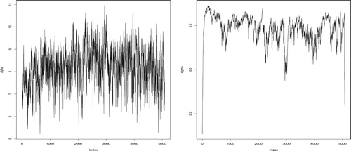
From Figure 2, we can see that $\left\{{\hat{\alpha }}_t\right\}$ and $\left\{{\hat{\sigma }}_t\right\}$ vary all the time, i.e., they cannot be constant. $\left\{{\hat{\alpha }}_t\right\}$ and $\left\{{\hat{\sigma }}_t\right\}$ are affected by the observed extreme values from previous days. Together with Table 2, one can see that (77(77) $\begin{array}{rl}{Q}_t& =\mu +{\sigma }_t{Y}_t^{1/{\alpha }_t},\end{array}$(77) )–(79(79) $\begin{array}{rl}\log {\alpha }_t& ={\gamma }_0+{\gamma }_1\log {\alpha }_{t-1}+{\gamma }_2\exp (-{\gamma }_3{Q}_{t-1}),\end{array}$(79) ) are good for describing the extreme movements in Dow Jones market. Additional analysis results and inference can be done using the fitted model as discussed in Zhao et al. (2018).

We will use the recovered value $Y_t$ to study extreme co-movements in the next section.

5.2. Extreme co-movements and risk contagions

Extreme co-movements refer to extreme values co-occur during a short time period. Risk contagions stand for that risk variables impact each other at extreme values. We use TQCC to study stock price extreme co-movements and risk contagions among Dow Jones' 30 stocks. In the literature, among many applications, Wu et al. (2012) illustrated the idea of studying the equity market index extreme co-movement using TQCC, and Deng and Zhang (2020) used TQCC to study haze extreme contagions in a vast region in China. In their applications, a generalised extreme value (GEV) fitting was implemented. In this section, we adopt a rank transformation using simulated data advocated in Zhang et al. (2011). The computation procedure is shown next.

Consider two stocks A and B among 28 stocks in Dow Jones 30. Denote their standardised negative return series derived from GARCH(1,1) fitting as ${ϵ}_t^A$ and ${ϵ}_t^B$, respectively; denote the sorted (from smallest to largest) series of the recovered $Y_t$ series from the fitted model (77(77) $\begin{array}{rl}{Q}_t& =\mu +{\sigma }_t{Y}_t^{1/{\alpha }_t},\end{array}$(77) ) as $Y_t^r$; denote $Y_t^A=Y_{\text{rank}\left({ϵ}_t^A\right)}^r$.

• For k = 1:1000,

  • Simulate a sequence of unit Fréchet random variables $Z_t$s;

  • Sort $\left\{Z_t\right\}$, and then denote the sorted sequence as $\left\{Y_t^s\right\}$;

  • Set $Y_t^B=Y_{\text{rank}\left({ϵ}_t^B\right)}^s$;

  • Set $(X_t,Y_t)=(Y_t^A,Y_t^B)$;

  • $u_n=min($the 97.5th percentile of $\left\{Y_t^A\right\}$, the 97.5th percentile of $\left\{Y_t^B\right\})$;

  • Compute $q_{.975,k}$ using TQCC formula (21(21) $\begin{array}{r}{q}_{u_n}=\frac{\begin{array}{l}\underset{1\le i\le n}{max}\{\frac{max(X_i,u_n)}{max(Y_i,u_n)}-1\}\\ +\underset{1\le i\le n}{max}\{\frac{max(Y_i,u_n)}{max(X_i,u_n)}-1\}\end{array}}{\begin{array}{l}\underset{1\le i\le n}{max}\left\{\frac{max(X_i,u_n)}{max(Y_i,u_n)}\right\}\\ \times \underset{1\le i\le n}{max}\left\{\frac{max(Y_i,u_n)}{max(X_i,u_n)}\right\}-1\end{array}}\end{array}$(21) );

  • Set $q_{AB}=\underset{1\le k\le 1000}{max}(q_{.975,k}$).

  Repeat the above process for all combinations of all 28 stocks.

For comparison, we also compute linear correlation coefficients $r_{AB}$ between two standardised time series ${ϵ}_t^A$ and ${ϵ}_t^B$. We use $q_{AB}$ and $r_{AB}$ to generate dendrograms in Figures 3 and 4.

Figure 3. Dendrograms based on TQCC (left) and linear correlation coefficients (right) using the complete linkage.

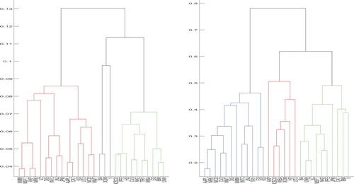
Figure 4. Dendrograms based on TQCC (left) and linear correlation coefficients (right) using the single linkage.

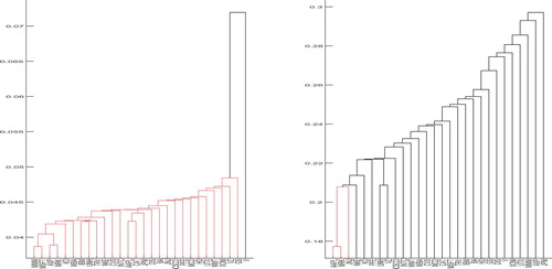
From Figures 3 and 4, we can immediately see that the stock clusters based on TQCC and the stock clusters based on correlation coefficients are different. It is clear correlation coefficients measure the relationship in the middle parts of the data. However, TQCC can reveal the relation in the tails. In Figure 3, the left panel based on TQCC can reveal the highest probability that given one stock price plunges within the left sub-branch of clustered compounds, one stock price also plunges within the right sub-branch of clustered compounds. In Figure 4, the left panel based on TQCC can reveal the smallest probability that given one stock price plunges within the left sub-branch of clustered compounds, one stock price also plunges within the right sub-branch of clustered compounds. Such information can help investors make better trading decisions and form better portfolios during volatile market movements.

6. Conclusions

In this review paper, a series of models and tail dependence measures have been discussed. These models can be applied to many research studies as long as extreme values and rare events are concerned. They can be used as alternative models and/or enhanced models to ARMA and GARCH models. They can be further extended to much more advanced models to meet the need for more complex data. In the literature, there are many other models that can be excellent candidate models for studying extremes, e.g., Brown-Resnick processes (Brown & Resnick, 1977; Huser & Davison, 2013). The new extreme value theory discussed in Section 3 can open a broad area of research. The autoregressive models with additive errors and competing errors and the autoregressive tail-index models can be extended to high order and high-dimensions. As to statistical inference, Bayesian inference of these models is also a promising research direction. In the literature of extreme value and moving maxima models, Kunihama et al. (2012) applied particle filter method to study moving maxima models. Idowu and Zhang (2017) applied a hybrid MCMC approach in a class of SM4R models. It can be expected that more researches using the discussed models will be rooted in many research areas.

Acknowledgments

The author thank Editor Jun Shao and two referees for their valuable comments. The work was partially supported by NSF-DMS-1505367 and NSF-DMS-2012298.

Disclosure statement

No potential conflict of interest was reported by the author(s).

Additional information

Funding

This work was partially supported by NSF - DMS-1505367 and NSF - DMS-2012298.

Notes on contributors

Zhengjun Zhang

Zhengjun Zhang is Professor of Statistics at the University of Wisconsin. His main research areas of expertise are in financial time series and rare event modeling, virtual standard currency, risk management, nonlinear dependence, asymmetric dependence, asymmetric and directed causal inference, gene-gene relationship in rare diseases.

Notes

1 If we let $d=d^{\prime }$, then the first three cases in the second column of Table 1 correspond to the serial asymptotic dependence index ${\lambda }_{d{d}_r}$.

References

- Beirlant, J., Goegebeur, Y., Segers, J., & Teugels, J. (2006). Statistics of extremes: Theory and applications. John Wiley & Sons.
- Brown, B. M., & Resnick, S. I. (1977). Extreme values of independent stochastic processes. Journal of Applied Probability, 14(4), 732–739. https://doi.org/10.2307/3213346
- Bücher, A., & Segers, J. (2017). On the maximum likelihood estimator for the generalized extreme-value distribution. Extremes, 20(4), 839–872. https://doi.org/10.1007/s10687-017-0292-6
- Cao, W., & Zhang, Z. (2020). New extreme value theory for maxima of maxima. Statistical Theory and Related Fields. https://doi.org/10.1080/24754269.2020.1846115
- Cartwright, D. E. (1958). On estimating the mean energy of sea waves from the highest waves in a record. Proceedings of the Royal Society of London, Series A, 247(1248), 22–28.https://doi.org/10.1098/rspa.1958.0168
- Castillo, E., Hadi, A. S., Balakrishnan, N., & Sarabia, J. M. (2005). Extreme value and related models with applications in engineering and science. Wiley Series in Probability and Statistics.
- Chen, Y., Wang, Z. C., & Zhang, Z. (2019). Mark to market value at risk. Journal of Econometrics, 208(1), 299–321. https://doi.org/10.1016/j.jeconom.2018.09.017
- Coles, S., Bawa, J., Trenner, L., & Dorazio, P. (2001). An introduction to statistical modeling of extreme values (vol. 208). Springer.
- Coles, S., Heffernan, J., & Tawn, J. (1999). Dependence measures for extreme value analyses. Extremes, 2(4), 339–365. https://doi.org/10.1023/A:1009963131610
- Coles, S. G., & Tawn, J. A. (1991). Modeling extreme multivariate events. Journal of the Royal Statistical Society, Series B, 53(2), 377–392.https://doi.org/10.1111/j.2517-6161.1991.tb01830.x
- Davis, R. A., & Resnick, S. I. (1989). Basic properties and prediction of max-ARMA processes. Advances in Applied Probability, 21(4), 781–803. https://doi.org/10.2307/1427767
- Davis, R. A., & Resnick, S. I. (1993). Prediction of stationary max-stable processes. The Annals of Applied Probability, 3(2), 497–525. https://doi.org/10.1214/aoap/1177005435
- de Haan, L. (1984). A spectral representation for max-stable processes. The Annals of Probability, 12(4), 1194–1204. https://doi.org/10.1214/aop/1176993148
- de Haan, L. (1985). Extremes in higher dimensions: The model and some statistics. In Proceedings of the 45th session international statistic institute. International Statistical Institute.
- de Haan, L. (1993). Extreme value statistics. In Janos Galambos, James Lechner, & Emil Simiu (Eds.), Extreme value theory and applications (pp. 93–122). Kluwer Academic.
- de Haan, L., & Ferreira, A. (2007). Extreme value theory: An introduction. Springer.
- de Haan, L., & Resnick, S. I. (1977). Limit theory for multivariate sample extremes. Zeitschrift für Wahrscheinlichkeitstheorie und Vrwandte Gebiete, 40(4), 317–337. https://doi.org/10.1007/BF00533086
- Deheuvels, P. (1983). Point processes and multivariate extreme values. Journal of Multivariate Analysis, 13(2), 257–272. https://doi.org/10.1016/0047-259X(83)90025-8
- Deng, L., & Zhang, Z. (2018). Assessing the features of extreme smog in China and the differentiated treatment strategy. Proceedings of the Royal Society A, 474, 220920170511. https://doi.org/10.1098/rspa.2017.0511
- Deng, L., & Zhang, Z. (2020). The haze extreme co-movements in Beijing-Tianjin-Hebei region and its extreme dependence pattern recognitions. Science Progress, 103(2), 36850420916315. https://doi.org/10.1177/0036850420916315
- Dey, D. K., & Yan, J. (2016). Extreme value modeling and risk analysis: Methods and applications, (EDS). Chapman & Hall/CRC.
- Drees, H., Ferreira, A., & de Haan, L. (2004). On maximum likelihood estimation of the extreme value index. Annals of Applied Probability, 14(3), 1179–1201. https://doi.org/10.1214/105051604000000279
- Embrechts, P., Klüppelberg, C., & Mikosch, T. (1997). Modelling extremal events for insurance and finance. Springer.
- Embrechts, P., Lindskog, F., & McNeil, A. (2003). Modelling dependence with copulas and applications to risk management. In S. Rachev (Ed.), Handbook of heavy tailed distributions in finance (pp. 329–384). Elsevier.
- Embrechts, P., McNeil, A., & Straumann, D. (2002). Correlation and dependence in risk management: Properties and pitfalls. In M. A. H. Dempster (Ed.), Risk management: Value at risk and beyond (pp. 176–223). Cambridge University Press.
- Embrechts, P., Resnick, S. I., & Samorodnitsky, G. (1999). Extreme value theory as a risk management tool. North American Actuarial Journal, 3(2), 30–41. https://doi.org/10.1080/10920277.1999.10595797
- Ferreira, H., & Ferreira, M. (2018). Estimating the extremal index through local dependence. Annales de l'Institut Henri Poincaré, Probabilités et Statistiques, 54(2), 587–605. https://doi.org/10.1214/16-AIHP815
- Finkenstädt, B., & Rootzén, H. E. (2004). Extreme values in finance, telecommunications, and the environment. Chapman & Hall/CRC.
- Fougéres, A.-L., Nolan, J. P., & Rootzén, H. (2009). Models for dependent extremes using stable mixtures. Scandinavian Journal of Statistics, 36, 42–59. https://doi.org/10.1111/j.1467-9469.2008.00613.x
- Galambos, J. (1987). Asymptotic theory of extreme order statistics (2nd ed.). Krieger.
- Hall, P., Peng, L., & Yao, Q. (2002). Moving-maximum models for extrema of time series. Journal of Statistical Planning and Inference, 103(1–2), 51–63. https://doi.org/10.1016/S0378-3758(01)00197-5
- Heffernan, J. E. (2001). A directory of coefficients of tail dependence. Extremes, 3(3), 279–290. https://doi.org/10.1023/A:1011459127975
- Heffernan, J. E., Tawn, J. A., & Zhang, Z. (2007). Asymptotically (in)dependent multivariate maxima of moving maxima processes. Extremes, 10(1-2), 57–82. https://doi.org/10.1007/s10687-007-0035-1
- Hsing, T. (1993). Extremal index estimation for a weakly dependent stationary sequence. The Annals of Statistics, 21(4), 2043–2071. https://doi.org/10.1214/aos/1176349409
- Huser, R., & Davison, A. C. (2013). Composite likelihood estimation for the Brown–Resnick process. Biometrika, 100(2), 511–518. https://doi.org/10.1093/biomet/ass089
- Hüsler, J., & Li, D. (2009). Testing asymptotic independence in bivariate extremes. Journal of Statistical Planning and Inference, 139(3), 990–998. https://doi.org/10.1016/j.jspi.2008.06.003
- Idowu, T., & Zhang, Z. (2017). An extended sparse max-linear moving model with application to high-frequency financial data. Statistical Theory and Related Fields, 1(1), 92–111. https://doi.org/10.1080/24754269.2017.1346852
- Joe, H. (2014). Dependence modeling with copulas. Chapman & Hall/CRC Monographs on Statistics & Applied Probability. Chapman & Hall/CRC.
- Kelly, B. (2014). The dynamic power law model. Extremes, 17(4), 557–583. https://doi.org/10.1007/s10687-014-0193-x
- Kunihama, T., Omori, Y., & Zhang, Z. (2012). Efficient estimation and particle filter for max-stable processes. Journal of Time Series Analysis, 33(1), 61–80. https://doi.org/10.1111/jtsa.2011.33.issue-1
- Leadbetter, M. R. (1983). Extremes and local dependence in stationary sequences. Zeitschrift für Wahrscheinlichkeitstheorie und Verwandte Gebiete, 65(2), 291–306. https://doi.org/10.1007/BF00532484
- Leadbetter, M. R., Lindgren, G., & Rootzén, H. (1983). Extremes and related properties of random sequences and processes. Springer Science & Business Media.
- Leadbetter, M. R., Weissman, I., de Haan, L., & Rootzén, H. (1989). On clustering of high values in statistically stationary seriess. In J. Sanson (Ed.), Proceedings of the 4th international meeting on statistical climatology. New Zealand Meteorological Service.
- Ledford, A. W., & Tawn, J. A. (1996). Statistics for near independence in multivariate extreme values. Biometrika, 83(1), 169–187. https://doi.org/10.1093/biomet/83.1.169
- Ledford, A. W., & Tawn, J. A. (1997). Modeling dependence within joint tail regions. Journal of the Royal Statistical Society: Series B (Statistical Methodology), 59(2), 475–499. https://doi.org/10.1111/rssb.1997.59.issue-2
- Loynes, R. M. (1965). Extreme values in uniformly mixing stationary stochastic processes. The Annals of Mathematical Statistics, 36(3), 993–999. https://doi.org/10.1214/aoms/1177700071
- Mao, G., & Zhang, Z. (2018). Stochastic tail index model for high frequency financial data with Bayesian analysis. Journal of Econometrics, 205(2), 470–487. https://doi.org/10.1016/j.jeconom.2018.03.019
- Martins, A. P., & Ferreira, H. (2014). Extremal properties of M4 processes. Test, 23(2), 388–408. https://doi.org/10.1007/s11749-014-0358-6
- Massacci, D. (2016). Tail risk dynamics in stock returns: Links to the macroeconomy and global markets connectedness. Management Science, 63(9), 1–18.https://doi.org/10.1287/mnsc.2016.2488
- McNeil, A. J., & Frey, R. (2000). Estimation of tail-related risk measures for heteroscedastic financial time series: An extreme value approach. Journal of Empirical Finance, 7(3–4), 271–300. https://doi.org/10.1016/S0927-5398(00)00012-8
- Meinguet, T. (2012). Maxima of moving maxima of continuous functions. Extremes, 15(3), 267–297. https://doi.org/10.1007/s10687-011-0136-8
- Mikosch, T., Embrechts, P., & Klüppelberg, C. (1997). Modelling extremal events for insurance and finance. Springer Verlag.
- Nandagopalan, S. (1990). Multivariate extremes and the estimation of the extremal index [PhD thesis]. University of North Carolina, Chapel Hill, Dept. Of Statistics.
- Nandagopalan, S. (1994). On the multivariate extremal index. Journal of Research of the National Institute of Standards and Technology, 99(4), 543–550. https://doi.org/10.6028/jres.099.052
- Naveau, P., Zhang, Z., & Zhu, B. (2011). An extension of max autoregressive models. Statistics and Its Interface, 4(2), 253–266. https://doi.org/10.4310/SII.2011.v4.n2.a19
- Newell, G. F. (1964). Asymptotic extremes for m-dependent random variables. The Annals of Mathematical Statistics, 35(3), 1322–1325. https://doi.org/10.1214/aoms/1177703288
- O'Brien, G. L. (1974). Limit theorems for the maximum term of a stationary process. Annals of Probability, 2(3), 540–545. https://doi.org/10.1214/aop/1176996673
- O'Brien, G. L. (1987). Extreme values for stationary and Markov sequences. Annals of Probability, 15(1), 281–291. https://doi.org/10.1214/aop/1176992270
- Peng, L. (1999). Estimation of the coefficient of tail dependence in bivariate extremes. Statistics & Probability Letters, 43(4), 399–409. https://doi.org/10.1016/S0167-7152(98)00280-6
- Pereira, L., & Fonseca, C. (2019). Statistical methods for assessing the contagion of spatial extreme events among regions. Communications in Statistics - Theory and Methods, 48(13), 3208–3218. https://doi.org/10.1080/03610926.2018.1473612
- Pickands, J. (1981). Multivariate extreme value distributions. In Proceedings 43rd session of the international statistical institute (Vol. 49, pp. 859–878).
- Reich, B. J., & Shaby, B. A. (2019). A spatial Markov model for climate extremes. Journal of Computational and Graphical Statistics, 28(1), 117–126. https://doi.org/10.1080/10618600.2018.1482764
- Resnick, S. I. (1987). Extreme values, regular variation, and point processes. Springer.
- Rodgers, J. L., & Nicewander, W. A. (1988). Thirteen ways to look at the correlation coefficient. American Statistician, 42(1), 59–66. https://doi.org/10.2307/2685263
- Salmon, F. (2012). The formula that killed wall street. Significance, 9(1), 16–20. https://doi.org/10.1111/j.1740-9713.2012.00538.x
- Salvadori, G., De Michele, C., Kottegoda, N. T., & Rosso, R. (2007). Extremes in nature: An approach using copulas. Springer. Complexity.
- Sibuya, M. (1959). Bivariate extreme statistics, I. Annals of the Institute of Statistical Mathematics, 11(2), 195–210.
- Smith, R. L. (1985). Maximum likelihood estimation in a class of nonregular cases. Biometrika, 72(1), 67–90. https://doi.org/10.1093/biomet/72.1.67
- Smith, R. L. (1990). Extreme value theory. Handbook of Applicable Mathematics, 7, 437–471.
- Smith, R. L., & Weissman, I. (1994). Estimating the extremal index. Journal of the Royal Statistical Society, Series B, 56(3), 515–528.
- Smith, R. L., & Weissman, I. (1996). Characterization and estimation of the multivariate extremal index. Technical report, University of North Carolina-Chapel Hill.
- Tang, R., Shao, J., & Zhang, Z. (2013). Sparse moving maxima models for tail dependence in multivariate financial time series. Journal of Statistical Planning and Inference, 143(5), 882–895. https://doi.org/10.1016/j.jspi.2012.11.008
- Tawn, J. A. (1988). Bivariate extreme value theory: Models and estimation. Biometrika, 75(3), 397–415.
- Weissman, I. (1994). On the extremal index of stationary sequences. Technical report, The Conference on Multivariate Extreme Value Estimation with Applications to Economics and Finance, Erasmus University, Rotterdam.
- Wu, J., Zhang, Z., & Zhao, Y. (2012). Study of the tail dependence structure in global financial markets using extreme value theory. Journal of Reviews on Global Economics, 1(1), 62–81.
- Yang, X., Frees, E. W., & Zhang, Z. (2011). A generalized beta copula with applications in modeling multivariate long-tailed data. Insurance: Mathematics and Economics, 49(2), 265–284. https://doi.org/10.1016/j.insmatheco.2011.04.007
- Zhang, Z. (2005). A new class of tail-dependent time series models and its applications in financial time series. Advances in Econometrics, 20(B), 323–358.
- Zhang, Z. (2008a). The estimation of M4 processes with geometric moving patterns. Annals of the Institute of Statistical Mathematics, 60(1), 121–150. https://doi.org/10.1007/s10463-006-0078-0
- Zhang, Z. (2008b). Quotient correlation: A sample based alternative to Pearson's correlation. The Annals of Statistics, 36(2), 1007–1030. https://doi.org/10.1214/009053607000000866
- Zhang, Z. (2009). On approximating max-stable processes and constructing extremal copula functions. Statistical Inference for Stochastic Processes, 12(1), 89–114. https://doi.org/10.1007/s11203-008-9027-2
- Zhang, Z., Qi, Y., & Ma, X. (2011). Asymptotic independence of correlation coefficients with application to testing hypothesis of independence. Electronic Journal of Statistics, 5, 342–372. https://doi.org/10.1214/11-EJS610
- Zhang, X., & Schwaab, B. (2017). Tail risk in government bond markets and ECB asset purchases. Working paper.
- Zhang, Z., & Smith, R. L. (2004). The behavior of multivariate maxima of moving maxima processes. Journal of Applied Probability, 41(4), 1113–1123. https://doi.org/10.1239/jap/1101840556
- Zhang, Z., & Smith, R. L. (2010). On the estimation and application of max-stable processes. Journal of Statistical Planning and Inference, 140(5), 1135–1153. https://doi.org/10.1016/j.jspi.2009.10.014
- Zhang, Z., Zhang, C., & Cui, Q. (2017). Random threshold driven tail dependence measures with application to precipitation data analysis. Statistica Sinica, 27(2), 685–709.https://doi.org/10.5705/ss.202015.0421
- Zhang, Z., & Zhu, B. (2016). Copula structured M4 processes with application to high-frequency financial data. Journal of Econometrics, 194(2), 231–241. https://doi.org/10.1016/j.jeconom.2016.05.004
- Zhao, Z., & Zhang, Z. (2018). Semi-parametric dynamic max-copula model for multivariate time series. Journal of the Royal Statistical Society: Series B (Statistical Methodology), 80(2), 409–432. https://doi.org/10.1111/rssb.12256
- Zhao, Z., Zhang, Z., & Chen, R. (2018). Modeling maxima with autoregressive conditional Fréchet model. Journal of Econometrics, 207, 2325–351. https://doi.org/10.1016/j.jeconom.2018.07.004
- Zhou, C. (2008). A two-step estimator of the extreme value index. Extremes, 11(3), 281–302. https://doi.org/10.1007/s10687-008-0058-2