Selecting baseline designs using a minimum aberration criterion when some two-factor interactions are important

ABSTRACT

This article considers the problem of selecting two-level designs under the baseline parameterisation when some two-factor interactions are important. We propose a minimum aberration criterion, which minimises the bias caused by the non-negligible effects. Using this criterion, a class of optimal designs can be further distinguished from one another, and we present an algorithm to find the minimum aberration designs among the D-optimal designs. Sixteen-run and twenty-run designs are summarised for practical use.

Keywords:

• Efficiency criterion
• fractional factorial design
• isomorphic design
• isomorphic model
• orthogonal array
• robust parameter design

1. Introduction

Fractional factorial designs, due to their run size economy, are widely used in many industrial or scientific areas. Particularly, two-level fractional factorial designs have received the most attention among practitioners. The experimenter often has some prior knowledge that allows a model containing certain important factorial effects to be postulated. While the most commonly used definition of factorial effects is given by a set of mutually orthogonal contrasts, which we refer to as the orthogonal parameterisation, an alternative considered in this article is the baseline parameterisation. Baseline parameterisation is more appropriate when each factor has a default or null state, and its usefulness has been increasingly recognised in recent years. For example, Yang and Speed (2002), Kerr (2006), and Banerjee and Mukerjee (2008) investigated factorial designs under the baseline parameterisation in the context of cDNA microarray experiments.

Firstly proposed by Fries and Hunter (1980), the minimum aberration is a popular criterion for selecting two-level fractional factorial designs. One justification for minimum aberration designs, given by Tang and Deng (1999), is that they provide a protection for the estimation of main effects by minimising the bias caused by the non-negligible interactions. The minimum aberration criterion can further distinguish orthogonal arrays, which are universally optimal (Cheng, 1980) under the main effect model. When the baseline parameterisation is under consideration, this idea leads to the minimum K-aberration criterion (Mukerjee & Tang, 2012).

In the present paper, we consider how to select baseline designs when, in addition to the main effects, some two-factor interactions are also important. Knowledge of important two-factor interactions arise in many applications. For example, in robust parameter designs, the estimation of interactions between the control and noise factors is crucial for the experimental objectives. Clearly, the minimum K-aberration criterion is not appropriate in this situation, so we propose a modified criterion that sequentially minimises the contamination caused by the non-negligible effects. The modified criterion is then used to further distinguish a class of optimal designs, and an algorithm is given to find out the best designs of sixteen and twenty runs.

This paper is organised as follows. Section 2 introduces notation and provides the definitions of the basic concepts, including factorial effects, minimum aberration criterion, and D-optimality criterion. Section 3 presents an algorithm for searching for minimum aberration baseline designs among D-optimal designs, which is then applied to designs of sixteen and twenty runs. Section 4 is the concluding section.

2. Notation and definitions

2.1. Factorial effects

Consider a two-level factorial involving m factors $F_1,F_2,\dots ,F_m$. Let ${\tau }_g$ denote the mean response at the level combination $g=(g_1,g_2,\dots ,g_m)$, where $g_i=0$ or 1 ($i=1,2,\dots ,m$). A factorial effect measures the impact on the mean response caused by the level changing of involved factor(s), and is defined by a treatment contrast. Let $\mathcal{G}$ be the collection of all possible level combinations. Under the most commonly used orthogonal parmeterisation, for a subset $w=\{i_1,i_2,\dots ,i_h\}$ of $S=\{1,2,\dots ,m\}$, the h-factor interaction $F_{i_1}{F}_{i_2}\cdots F_{i_h}$ (the main effect if h = 1) is (1) ${\beta }_w=\frac{1}{2^m}\sum _{g\in \mathcal{G}}{\tau }_g(-1{)}^{\sum _{j=1}^h{g}_{i_j}}.$(1)  We let ${\beta }_{\varphi }=2^{-m}\sum _{\mathcal{G}}{\tau }_g$, the grand mean. In the present paper, we focus on the alternative baseline parameterisation. For convenience, here and after we will also denote ${\tau }_{(1,1,0,\dots ,0)}$ by ${\tau }_{12}$, and similar notation applies to any other ${\tau }_g$. Under the baseline parameterisation, the main effect of $F_i$ is ${\theta }_i={\tau }_i-{\tau }_{\varphi }$, and the two-factor interaction $F_i{F}_j$ is ${\theta }_{ij}={\tau }_{ij}-{\tau }_i-{\tau }_j+{\tau }_{\varphi }$. More generally, for a subset $w=\{i_1,i_2,\dots ,i_h\}$ of S, the h-factor interaction $F_{i_1}{F}_{i_2}\dots F_{i_h}$ under the baseline parameterisation is (2) ${\theta }_w=\sum _{u\subseteq w}{\tau }_u(-1{)}^{|w|-|u|}.$(2) where $|\cdot |$ stands for the cardinality of a set. We let ${\theta }_{\varphi }={\tau }_{\varphi }$. The main distinction between the orthogonal and baseline parameterisations is that the former defines the effects in an overall sense, while the later defines the effects in a way that the non-involved factors are kept at their baseline levels.

The baseline parameterisation arises naturally in the experiments in which each factor has a default or null state. For example, in a toxicological study, each factor is a toxin, and each treatment is a mix of several toxins. Then, absence and presence can be represented by levels 0 and 1, respectively. The baseline parameterisation is also more appropriate if only a few factors are allowed to change their settings. Consider a situation in which the experimenter wants to improve an industrial process by changing only a few factors' current setting. Let levels 0 and 1 be the current and new settings, respectively. In this case, the baseline effects are more relevant and useful to the experimenter.

2.2. Minimum aberration criteria

An N-run and m-factor design $D=[g_{ij}]$ with $g_{ij}=0$ or 1 is represented by an $N\times m$ matrix in which a row corresponds to an experimental run and a column to a factor. Let Y be the vector of N observations. Under design D, the main effect model is $E(Y)=W_1{\mathit{\theta }}_1,$where $W_1=[\mathbf{1}D]$ with $\mathbf{1}$ being the all-ones vector, and ${\mathit{\theta }}_1=({\theta }_{\varphi },{\theta }_1,\dots ,{\theta }_m)$. We assume as usual that all observations are uncorrelated and have a common variance. If the interactions cannot be ignored, the true model under D is (3) $E(Y)=W_1{\mathit{\theta }}_1+W_2{\mathit{\theta }}_2+\cdots +W_m{\mathit{\theta }}_m,$(3) where for $j=2,\dots ,m$, ${\mathit{\theta }}_j$ is the vector of all interactions involving j factors and $W_j$ is the corresponding matrix obtained by taking all j-column products from D. Let ${\hat{\mathit{\theta }}}_1=(W_1^T{W}_1{)}^{-1}{W}_1^{T}Y$ be the least square estimator of ${\mathit{\theta }}_1$ under the main effect model, which is biased under model (3(3) $E(Y)=W_1{\mathit{\theta }}_1+W_2{\mathit{\theta }}_2+\cdots +W_m{\mathit{\theta }}_m,$(3) ), and the bias can be found by $\mathrm{bias}({\hat{\mathit{\theta }}}_1,{\mathit{\theta }}_1)=B_2{\mathit{\theta }}_2+\cdots +B_m{\mathit{\theta }}_m,$where $B_j=(W_1^T{W}_1{)}^{-1}{W}_1^T{W}_j$, $j=2,\dots ,m$. The contribution of ${\mathit{\theta }}_j$ to the bias is $B_j{\mathit{\theta }}_j$, where ${\mathit{\theta }}_j$ is unknown and $B_j$ depends on the design. To minimise the bias in the estimation of main effects caused by the non-negligible j-factor interactions, Mukerjee and Tang (2012) proposed the minimum K-aberration criterion, which selects designs by sequentially minimising $K_j=\mathrm{tr}({B_j^{\ast }}^T{B}_j^{\ast })$, a size measure of $B_j^{\ast }$, where $B_j^{\ast }$ is the matrix obtained by deleting the first row of $B_j$. Following the same path, we consider the model that contains the intercept, all main effects and some two-factor interactions that are presumably important, as given by (4) $E(Y)=W\mathit{\theta },$(4) where $\mathit{\theta }$ contains all the main effects and the important two-factor interactions, and W is $W_1$ plus the corresponding columns of $W_2$. If the effects outside this model cannot be ignored, the true model is (5) $E(Y)=W\mathit{\theta }+W_2^{\ast }{\mathit{\theta }}_2^{\ast }+W_3{\mathit{\theta }}_3+\cdots +W_m{\mathit{\theta }}_m,$(5) where ${\mathit{\theta }}_2^{\ast }$ contains the non-important two-factor interactions and $W_2^{\ast }$ is the corresponding matrix. Let $\hat{\mathit{\theta }}=(W^{T}W{)}^{-1}{W}^{T}Y$ be the least square estimator of $\mathit{\theta }$ under model (4(4) $E(Y)=W\mathit{\theta },$(4) ), which is biased under model (5(5) $E(Y)=W\mathit{\theta }+W_2^{\ast }{\mathit{\theta }}_2^{\ast }+W_3{\mathit{\theta }}_3+\cdots +W_m{\mathit{\theta }}_m,$(5) ), and the bias can be found by $\mathrm{bias}(\hat{\mathit{\theta }},\mathit{\theta })=C_2{\mathit{\theta }}_2+\cdots +C_m{\mathit{\theta }}_m,$where $C_2=(W^{T}W{)}^{-1}{W}^T{W}_2^{\ast }$ and $C_j=(W^{T}W{)}^{-1}{W}^T{W}_j$, for $j=3,\dots ,m$. We now define a new criterion, called minimum Q-aberration criterion, which is used to select baseline designs under model (4(4) $E(Y)=W\mathit{\theta },$(4) ). Let $Q_j=\mathrm{tr}(C_j^T{C}_j)$, $j=2,\dots ,m$, and $Q(D)=(Q_2,\dots ,Q_m)$, the Q-aberration of D. For any two competing designs D and $D^{\prime }$, let s be the smallest integer such that D and $D^{\prime }$ have different $Q_s$ values. If D has smaller $Q_s$ value than $D^{\prime }$, we say D has less Q-aberration than $D^{\prime }$. A design is said to have minimum Q-aberration if there is no other design that has less Q-aberration than it.

Though similar, our approach is slightly different from that of Mukerjee and Tang (2012). The situations considered in Mukerjee and Tang (2012) are screening experiments and they therefore focussed on the estimation of main effects by excluding the intercept from consideration. Our situations are different. If we are able to specify some important two-factor interactions, then we are reasonably confident that the model containing the intercept, main effects and important two-factor interactions is approximately correct. This means that all the parameters in the specified model are important and should be estimated to the best extent possible.

2.3. Optimality criterion

When a model is postulated, the experimenter would like to find designs that enjoy certain optimality properties. The optimality criterion considered in this article is the D-efficiency. Consider model (4(4) $E(Y)=W\mathit{\theta },$(4) ), the D-efficiency criterion is to minimise $[\det (W^{T}W){]}^{-1/p}$, where p is the number of columns of W, which minimises the volume of the confidence region of $\mathit{\theta }$.

In a similar study, Ke and Tang (2003) considered regular designs under the orthogonal parameterisation. Regular designs are guaranteed to have the full efficiency provided they can estimate the fitted model.

Let $E(Y)=X\mathit{\beta }$ be the counterpart model of model (4(4) $E(Y)=W\mathit{\theta },$(4) ) under the orthogonal parameterisation. That is, the column of X that is associated with ${\beta }_i$ is the ith column of 2D−1, and the column associated with ${\beta }_{ij}$ is the Hadamard product of the ith and jth columns of 2D−1. According to C. Y. Sun and Tang (2020), the two models are equivalent. We have the following lemma, which is a special case of Theorem 3 of C. Y. Sun and Tang (2020).

Lemma 2.1

Consider model (4(4) $E(Y)=W\mathit{\theta },$(4) ). If D is a baseline design such that X is orthogonal, then it is D-optimal among all competing designs. Moreover, such a D minimises $\mathrm{var}({\hat{\theta }}_w)$ if there is no ${\theta }_u$ in the model such that w is a proper subset of u.

C. Y. Sun and Tang (2020) considered a model that is more general than model (4(4) $E(Y)=W\mathit{\theta },$(4) ), and they call ${\theta }_w$ a cap effect if there is no ${\theta }_u$ in the model such that w is a proper subset of u. For example, under the main effect model, all main effect are cap effects. Under model (4(4) $E(Y)=W\mathit{\theta },$(4) ), the important two-factor interactions are cap effects, so are the main effects of those factors that are not involved in any important two-factor interaction. As indicated by C. Y. Sun and Tang (2020), the cap effects should be the first in line to be tested for their significance when one seeks a simpler model in the analysis stage.

3. Searching for best baseline designs

In this section, we present an algorithm to search for minimum Q-aberration designs among the D-optimal designs under model (4(4) $E(Y)=W\mathit{\theta },$(4) ). The first two subsections introduce two necessary concepts, and the algorithm and results are given in the third subsection. The last subsection provides an illustrative example.

3.1. Design isomorphism

Under the orthogonal parameterisation, two designs are isomorphic if one can be obtained from the other by (i) row permutation, (ii) column permutation, (iii) level permutation, or any combination of these three. Mukerjee and Tang (2012) suggest a different definition of isomorphism for baseline designs, which is similarly defined except for that level permutations are not allowed, since the two levels are not symmetric under the baseline parameterisation. To avoid ambiguity, we call the former the combinatorial isomorphism. Clearly, two designs are combinatorially isomorphic if they are isomorphic, but the converse is not true. A two-level orthogonal array is an $N\times m$ matrix with entries from a set of two symbols, such that for every two columns, all level-combinations appear equally often. A complete catalogue of combinatorially non-isomorphic two-level orthogonal arrays with $N\le 20$ are available in D. X. Sun et al. (2008). A more comprehensive catalogue of orthogonal arrays can be found at http://www.pietereendebak.nl/oapackage/series.html. Based on the catalogue given by D. X. Sun et al. (2008), we will conduct a complete search on the class of baseline designs that are orthogonal arrays, called orthogonal baseline designs for convenience.

3.2. Non-isomorphic models

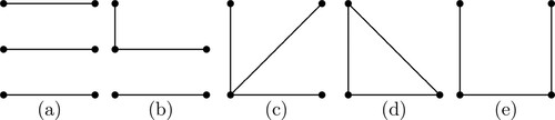
There are a huge number of models that are given by (4(4) $E(Y)=W\mathit{\theta },$(4) ). Among these models, many share the same structures. The graph theory is a convenient tool to deal with the model structure. For example, the models with $\mathit{\theta }=({\mathit{\theta }}_1,{\theta }_{12},{\theta }_{34})$ and $\mathit{\theta }=({\mathit{\theta }}_1,{\theta }_{12},{\theta }_{13})$ can be represented by the graphs in Figure 2(a,b), respectively. In such a graph, a vertex stands for a factor, and a line connects two vertices if their interaction is included in the model. Note that the factors (vertices) not involved in any important two-factor interaction do not appear in the graph. We say two models are isomorphic if one can be obtained from the other by relabelling the factors. Let k denote the number of two-factor interactions in model (4(4) $E(Y)=W\mathit{\theta },$(4) ). All non-isomorphic models for different values of $k\le 3$ are given in Figures 1–3. The cases for $k\ge 4$ are not considered because of the large number of possible models, and also because k tends to be small in practice due to the effect sparsity principle (Wu & Hamada, 2011, pp. 173).

Figure 1. Model containing one interaction (k = 1).

Figure 2. Models containing two interactions (k = 2).

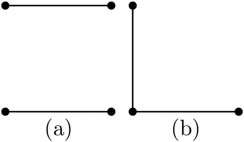
Figure 3. Models containing three interactions (k = 3).

For a given graph and a design matrix, there are many possible ways to assign the columns to the vertexes, and the resulting design efficiency and Q-aberration may be different. To conduct a complete search, all possible column-to-vertex assignments need to be considered, as we will see in the next subsection.

3.3. Algorithm and results

Suppose N experimental runs are allowed to study m factors under a model whose structure is given by a graph R. Let $D_1,\dots ,D_n$ be the combinatorially non-isomorphic $N\times m$ orthogonal arrays in the catalogue given by D. X. Sun et al. (2008), where each $D_i$ consists of 1 and $-1$. The algorithm proceeds as follows, starting with i = 1.

1. Set $D_i=(D_i+1)/2$. If i = 1, set $D_{best}=D_1$ and $Q_{best}=Q(D_{best})$.

2. Switch the two levels 0 and 1 for a subset of factors.

3. For the resulting baseline design matrix, assign the columns to the vertexes of R.

4. Obtain the resulting model matrix W and compute the D-efficiency. Compare $D_i$ with $D_{best}$. If (i) $D_i$ has better D-efficiency, or (ii) $D_i$ has the same D-efficiency and less Q-aberration, then set $D_{best}=D_i$, and $Q_{best}=Q(D_{best})$.

5. Go back to step 3 with another possible column-to-vertex assignment. When all possible assignments are considered, go back to step 2 with another possible subset. When all possible subsets are considered, go back to step 1 with $D_{i+1}$.

This algorithm finds a minimum Q-aberration design that is D-optimal among all orthogonal baseline designs. Such a design may not be unique, and $D_{best}$ is the first one found by the algorithm. In our algorithm, some isomorphic designs may be considered more than once, but no orthogonal baseline design will be missed. If a complete catalogue of non-isomorphic orthogonal baseline designs is available, a more efficient algorithm can be presented.

We apply this algorithm to all models given by Figures 1–3 and the $D_{best}$ for N = 16 and 20 are summarised in Tables 1–6. For N = 20, the tables only cover the designs with $m\le 7$, since the required computation increases rapidly when m>7. In each of these tables, the second, third, and the fourth columns indicate, which $D_i$ should be used, which two-factor interactions should be included in the model, and for which design columns the level switching should be conducted, respectively. The A-efficiency of $D_{best}$ is also calculated for the readers' information, where the A-efficiency is $\mathrm{tr}(W^{T}W{)}^{-1}$, but it is not used in the search algorithm.

Table 1. Sixteen-run MA baseline designs for the model with k = 1.

m	i	Interaction	Switched	D-efficiency	A-efficiency	($Q_2$, $Q_3$, $Q_4$)
4	3	$(1,2)$	None	0.25	2.88	(2.81, 1.16, 0.11)
5	3	$(1,5)$	1	0.25	3.19	(5.06, 2.80, 0.55)
6	4	$(2,4)$	1	0.25	3.50	(8.44, 6.08, 1.81)
7	5	$(1,6)$	1, 6	0.25	3.81	(12.38, 11.33, 4.97)
8	4	$(1,8)$	1, 8	0.25	4.13	(16.88, 19.12, 11.5)
9	3	$(1,9)$	1, 6	0.25	4.44	(24.50, 33.16, 24.09)
10	3	$(2,10)$	2, 5, 8	0.25	4.75	(32.69, 49.70, 39.75)
11	3	$(1,11)$	3, 4, 7	0.25	5.06	(41.44, 72.08, 67.34)
12	1	$(4,9)$	1, 2, 3, 12	0.25	5.38	(51.88, 100.44, 102.38)
13	1	$(2,12)$	1, 2, 3, 12, 13	0.25	5.69	(62.88, 135.88, 156.14)
14	1	$(1,14)$	1, 2, 3, 12, 13, 14	0.25	6.00	(75.00, 179.00, 228.50)

Table 2. Sixteen-run MA baseline designs for the models with k = 2.

m	Model	i	Interactions	Switched	D-efficiency	A-efficiency	($Q_2$, $Q_3$, $Q_4$)
4	2(a)	3	$(1,2),(3,4)$	None	0.30	4.44	(2.25, 1.31, 0.13)
	2(b)	3	$(1,2),(1,3)$	None	0.30	4.44	(2.25, 1.47, 0.16)
5	2(a)	4	$(1,2),(3,4)$	None	0.30	4.75	(4.50, 3.69, 0.78)
	2(b)	3	$(1,5),(2,5)$	1	0.30	4.75	(4.50, 3.19, 0.72)
6	2(a)	4	$(2,4),(3,5)$	1	0.29	5.06	(7.88, 7.27, 2.45)
	2(b)	4	$(2,4),(3,4)$	1	0.29	5.06	(7.88, 7.05, 2.36)
7	2(a)	4	$(4,6),(5,7)$	1, 6	0.29	5.38	(12.38, 13.25, 6.19)
	2(b)	5	$(1,6),(1,7)$	1, 6	0.29	5.38	(11.81, 13.50, 6.66)
8	2(a)	2	$(2,7),(6,8)$	1, 6	0.28	5.69	(18.88, 23.56, 13.31)
	2(b)	2	$(6,7),(6,8)$	1, 6	0.28	5.69	(17.44, 22.23, 13.95)
9	2(a)	2	$(4,8),(5,9)$	1, 2, 3	0.28	6.00	(25.94, 38.00, 26.64)
	2(b)	2	$(4,8),(4,9)$	1, 2, 3	0.28	6.00	(25.94, 37.75, 26.36)
10	2(a)	3	$(2,10),(4,9)$	2, 5, 8	0.28	6.31	(35.00, 59.61, 50.29)
	2(b)	3	$(2,10),(3,10)$	2, 5, 8	0.28	6.31	(35.00, 59.23, 49.39)
11	2(a)	1	$(4,8),(5,10)$	1, 2, 3	0.28	6.62	(45.75, 86.00, 79.62)
	2(b)	1	$(4,8),(4,9)$	1, 2, 3	0.28	6.62	(45.75, 86.00, 80.12)
12	2(a)	1	$(4,9),(5,10)$	1, 2, 3, 12	0.27	6.94	(57.06, 121.55, 129.09)
	2(b)	1	$(4,9),(4,10)$	1, 2, 3, 12	0.27	6.94	(57.06, 121.42, 128.84)
13	2(a)	1	$(2,12),(4,11)$	1, 2, 3, 12, 13	0.27	7.25	(69.50, 164.50, 196.81)
	2(b)	1	$(2,12),(2,13)$	1, 2, 3, 12, 13	0.27	7.25	(69.50, 164.50, 196.94)

Table 3. Sixteen-run MA baseline designs for the models with k = 3.

m	Model	i	Interactions	Switched	D-efficiency	A-efficiency	($Q_2$, $Q_3$, $Q_4$)
4	3(a)	–	–	–	–	–	–
	3(b)	–	–	–	–	–	–
	3(c)	3	$(1,2),(1,3),(1,4)$	None	0.35	6.00	(1.69, 1.94, 0.25)
	3(d)	3	$(1,2),(1,3),(2,4)$	None	0.35	6.00	(1.69, 1.78, 0.22)
	3(e)	3	$(1,2),(1,3),(2,3)$	None	0.35	6.00	(1.69, 1.94, 0.25)
5	3(a)	–	–	–	–	–	–
	3(b)	4	$(1,2),(1,3),(4,5)$	None	0.34	6.31	(3.94, 4.47, 1.04)
	3(c)	3	$(1,5),(2,5),(3,5)$	1	0.34	6.31	(3.94, 3.73, 0.89)
	3(d)	4	$(1,2),(1,3),(2,4)$	None	0.34	6.31	(3.94, 4.56, 1.19)
	3(e)	4	$(1,2),(1,3),(2,3)$	None	0.34	6.31	(3.94, 4.66, 1.35)
6	3(a)	3	$(1,4),(2,5),(3,6)$	1, 4	0.33	6.63	(7.88, 8.62, 2.95)
	3(b)	4	$(2,4),(2,5),(3,6)$	1	0.33	6.63	(7.31, 8.61, 3.20)
	3(c)	4	$(2,4),(2,5),(2,6)$	1	0.33	6.63	(7.31, 8.80, 3.33)
	3(d)	4	$(2,4),(2,5),(3,4)$	1	0.33	6.63	(7.31, 8.39, 3.11)
	3(e)	4	$(2,4),(2,5),(4,5)$	2	0.33	6.63	(8.75, 9.91, 3.83)
7	3(a)	5	$(1,6),(2,5),(3,7)$	1	0.32	6.94	(14.12, 18.00, 8.91)
	3(b)	5	$(1,6),(1,7),(2,5)$	1, 6	0.32	6.94	(12.69, 16.70, 8.48)
	3(c)	2	$(1,7),(2,7),(3,7)$	1, 6	0.32	6.94	(12.38, 13.80, 5.27)
	3(d)	4	$(4,6),(4,7),(5,6)$	1, 6	0.32	6.94	(11.81, 14.75, 7.44)
	3(e)	5	$(1,6),(1,7),(6,7)$	1	0.32	6.94	(14.12, 18.64, 9.92)
8	3(a)	16	$(1,5),(2,3),(7,8)$	1, 5, 8	0.31	7.25	(20.62, 29.28, 17.53)
	3(b)	7	$(1,7),(2,7),(3,8)$	3, 4, 7	0.31	7.25	(19.69, 27.23, 15.88)
	3(c)	1	$(1,8),(2,8),(3,8)$	1, 2, 3	0.31	7.25	(18.00, 23.12, 11.31)
	3(d)	2	$(2,7),(6,7),(6,8)$	1, 6	0.31	7.25	(18.31, 25.92, 16.09)
	3(e)	5	$(1,7),(1,8),(7,8)$	1, 6	0.31	7.25	(22.06, 32.06, 19.44)
9	3(a)	2	$(4,8),(5,9),(6,7)$	1, 2, 3	0.31	7.56	(26.81, 43.77, 32.45)
	3(b)	1	$(2,8),(4,8),(6,9)$	1, 2, 3	0.31	7.56	(27.38, 42.75, 28.75)
	3(c)	1	$(2,8),(4,8),(6,8)$	1, 2, 3	0.31	7.56	(27.38, 42.25, 28.00)
	3(d)	2	$(4,8),(4,9),(5,9)$	1, 2, 3	0.31	7.56	(26.81, 43.27, 31.89)
	3(e)	5	$(1,6),(1,9),(6,9)$	1, 6, 9	0.31	7.56	(30.56, 51.09, 38.10)
10	3(a)	1	$(4,8),(5,10),(7,9)$	1, 2, 3	0.30	7.88	(37.88, 68.33, 56.28)
	3(b)	1	$(4,8),(4,9),(5,10)$	1, 2, 3	0.30	7.88	(37.88, 68.20, 56.28)
	3(c)	1	$(4,8),(4,9),(4,10)$	1, 2, 3	0.30	7.88	(37.88, 67.95, 56.28)
	3(d)	1	$(4,8),(4,9),(6,8)$	1, 2, 3	0.30	7.88	(37.88, 68.08, 56.28)
	3(e)	3	$(6,9),(6,10),(9,10)$	2, 5, 8	0.30	7.88	(41.62, 76.97, 63.80)
11	3(a)	1	$(4,8),(5,10),(6,11)$	1, 2, 3	0.30	8.19	(49.50, 100.25, 95.38)
	3(b)	1	$(4,8),(4,9),(5,10)$	1, 2, 3	0.30	8.19	(49.50, 100.25, 95.88)
	3(c)	1	$(4,8),(4,9),(4,10)$	1, 2, 3	0.30	8.19	(49.50, 100.25, 96.88)
	3(d)	1	$(4,8),(4,9),(6,8)$	1, 2, 3	0.30	8.19	(49.50, 100.25, 96.38)
	3(e)	3	$(1,6),(1,9),(6,9)$	3, 4, 7	0.30	8.19	(53.25, 112.45, 111.03)
12	3(a)	1	$(4,9),(5,10),(6,8)$	1, 2, 3, 12	0.30	8.50	(62.25, 142.62, 155.75)
	3(b)	1	$(4,9),(4,10),(7,8)$	1, 2, 3, 12	0.30	8.50	(62.25, 142.50, 155.50)
	3(c)	1	$(4,9),(4,10),(4,11)$	1, 2, 3, 12	0.30	8.50	(62.25, 142.25, 155.00)
	3(d)	1	$(4,9),(4,10),(5,10)$	1, 2, 3, 12	0.30	8.50	(62.25, 142.38, 155.25)
	3(e)	2	$(1,6),(1,10),(6,9)$	1, 6, 9, 10	0.30	8.50	(66.00, 156.00, 177.00)

Note: “–” means that there is no such a model for the given m.

Table 4. Twenty-run MA baseline designs for the model with k = 1.

m	i	Interaction	Switched	D-efficiency	A-efficiency	($Q_2$, $Q_3$, $Q_4$)
4	1	$(1,2)$	1, 2, 4	0.20	2.39	(2.78, 1.07, 0.00)
5	8	$(3,5)$	None	0.20	2.70	(5.24, 2.62, 0.26)
6	70	$(2,5)$	1, 2, 5	0.20	3.02	(8.56, 5.78, 1.27)
7	471	$(4,6)$	1, 3, 4, 6, 7	0.21	3.35	(12.55, 11.26, 4.22)

Table 5. Twenty-run MA baseline designs for the models with k = 2.

m	Model	i	Interactions	Switched	D-efficiency	A-efficiency	($Q_2$, $Q_3$, $Q_4$)
4	2(a)	1	$(1,2),(3,4)$	1, 2, 4	0.25	3.80	(2.37, 1.22, 0.00)
	2(b)	1	$(1,2),(1,3)$	1, 2, 4	0.25	3.75	(2.30, 1.50, 0.00)
5	2(a)	10	$(1,2),(3,5)$	2, 3, 5	0.25	4.16	(5.21, 3.57, 0.29)
	2(b)	8	$(1,5),(3,5)$	None	0.25	4.13	(4.96, 3.10, 0.34)
6	2(a)	67	$(1,5),(4,6)$	2, 3, 4, 5	0.24	4.53	(8.83, 7.74, 2.34)
	2(b)	47	$(2,6),(3,6)$	1,2, 3, 5, 6	0.24	4.52	(8.62, 7.02, 1.93)
7	2(a)	403	$(1,4),(3,7)$	2, 3, 4, 6, 7	0.24	4.94	(13.42, 14.13, 6.20)
	2(b)	451	$(1,5),(2,5)$	3, 4, 5, 7	0.24	4.92	(13.23, 15.33, 7.83)

Table 6. Twenty-run MA baseline designs for the models with k = 3.

m	Model	i	Interactions	Switched	D-efficiency	A-efficiency	($Q_2$, $Q_3$, $Q_4$)
4	3(a)	–	–	–	–	–	–
	3(b)	–	–	–	–	–	–
	3(c)	1	$(1,2),(1,3),(1,4)$	1, 2, 4	0.29	5.13	(1.80, 1.98, 0.00)
	3(d)	1	$(1,2),(1,3),(2,4)$	1, 2, 4	0.29	5.19	(1.85, 1.69, 0.00)
	3(e)	1	$(1,2),(1,3),(2,3)$	None	0.29	5.11	(2.14, 2.18, 0.31)
5	3(a)	–	–	–	–	–	–
	3(b)	10	$(1,2),(3,5),(4,5)$	1, 4, 5	0.29	5.71	(4.84, 4.71, 0.54)
	3(c)	8	$(1,5),(2,5),(3,5)$	1,2 ,5	0.28	5.58	(4.75, 4.67, 0.88)
	3(d)	10	$(1,2),(1,4),(4,5)$	1,4 ,5	0.29	5.62	(4.84, 4.21, 0.36)
	3(e)	10	$(1,2),(1,5),(2,5)$	None	0.28	5.55	(5.12, 4.33, 0.89)
6	3(a)	57	$(1,4),(2,5),(3,6)$	1, 4, 6	0.28	6.20	(8.71, 9.56, 3.35)
	3(b)	46	$(1,6),(3,4),(3,5)$	1, 3, 5	0.28	6.09	(8.92, 9.85, 3.31)
	3(c)	69	$(1,5),(4,5),(5,6)$	None	0.28	6.03	(8.67, 9.60, 2.92)
	3(d)	67	$(1,5),(4,6),(5,6)$	2, 3, 4, 5	0.28	6.05	(8.71, 9.29, 3.04)
	3(e)	58	$(4,5),(4,6),(5,6)$	4, 5	0.28	5.99	(9.08, 10.35, 6.66)
7	3(a)	429	$(2,7),(3,6),(4,5)$	2	0.27	6.55	(14.07, 16.70, 7.32)
	3(b)	334	$(1,5),(2,6),(5,7)$	1, 2, 4, 5, 7	0.27	6.53	(13.91, 17.15, 8.00)
	3(c)	430	$(1,5),(1,6),(1,7)$	1, 7	0.27	6.48	(13.89, 15.91, 6.82)
	3(d)	429	$(3,5),(3,6),(4,5)$	1, 2, 4	0.27	6.55	(13.68, 17.57, 7.90)
	3(e)	425	$(4,6),(4,7),(6,7)$	5, 6, 7	0.27	6.48	(14.27, 16.33, 6.52)

Note: “–” means that there is no such a model for the given m.

Consider Lemma 2.1. For a given N, m, and a model structure, if there exists a baseline design such that X is orthogonal, then step 4 in the algorithm can be replaced by step $4^{\prime }$ below to save the computation. For example, when N = 16 and $k\le 3$, we use it to obtain Tables 1–3.

4'.	Obtain the counterpart model matrix X under the orthogonal parameterisation. If X is orthogonal and $D_i$ has less Q-aberration than $D_{best}$, then set $D_{best}=D_i$ and $Q_{best}=Q(D_i)$ .

Finally, we note that by Lemma 2.1, all the designs given by Tables 1–3 are D-optimal among all competing designs because the model matrix X has orthogonal columns. The designs in Tables 4–6 are D-optimal among all 20-run orthogonal arrays as our search is complete.

3.4. An example

We consider a cake baking experiment in which the experimenter wants to improve a cake recipe. There are eight factors: baking time (Time), baking temperature (Temp), the number of eggs, and the amounts of baking powder, flour, sugar, milk (M) and butter. For each factor, there are two settings: the currently used setting and the new setting. The experimenter can only afford a sixteen-run design. Two two-factor interactions are important based on prior knowledge: the temperature-by-time and milk-by-time interactions. In this case, k = 2, N = 16, and m = 8, and the model has the structure 2(b). By Table 2, the experimenter should start with $D_2$ and set $D_2=(D_2+1)/2$, and then switch the two levels 0 and 1 for columns 1 and 6. Next, the factors Time, Temp, and M have to be assigned to columns 6, 7, and 8 (or 6, 8, and 7), respectively. All the remaining factors can be randomly assigned to the other columns. By Lemma 2.1, this design guarantees D-optimality among all competing designs; and except for the main effects of Time, Temp, and M, each of the other effects can be estimated with a minimal variance. Among all optimal designs, this design also minimises the contamination to the estimation of $\mathit{\theta }$ caused by non-negligible effects.

4. Concluding remarks

In our algorithm, we first use D-optimality, and then use the minimum aberration. One can also do it in a reversed order. In fact, the designs that have minimum Q-aberration among all competing designs are generally not orthogonal arrays. Examples are Rechtschaffner designs; see C. Y. Sun and Tang (2020) for details. In our search algorithm, the D-optimality can also be replaced by the A-optimality if one wishes, which is to minimise the A-efficiency and thus minimises $\sum _w\mathrm{var}({\hat{\theta }}_w)$. One possible future work is to develop an efficient algorithm that allows us to obtain more designs without complete search. Li et al. (2014) considered this problem for main effects models. Some of the ideas in that paper should be useful for the situations where some two-factor interactions are important.

Disclosure statement

No potential conflict of interest was reported by the author(s).

Additional information

Funding

This work was supported by Natural Sciences and Engineering Research Council of Canada [Discovery Grant].

Notes on contributors

Anqi Chen

Anqi Chen, is currently studying biostatistics, working towards her PhD at Simon Fraser University. She obtained her BSc and MSc in 2017 and 2019, respectively, from the same institution.

Cheng-Yu Sun

Cheng-Yu, a PhD student in statistics, is working towards his PhD at Simon Fraser University. His research interest is in experimental design, and has published one paper prior to this one.

Boxin Tang

Boxin Tang, a professor of statistics at Simon Fraser University, conducts research in the area of experimental design. He is an elected Fellow of ASA and IMS, and has published more than 60 papers in refereed journals.

References

- Banerjee, T., & Mukerjee, R. (2008). Optimal factorial designs for cDNA microarray experiments. The Annals of Applied Statistics, 2(1), 366–385. https://doi.org/10.1214/07-AOAS144
- Cheng, C. S. (1980). Orthogonal arrays with variable numbers of symbols. The Annals of Statistics, 8(2), 447–453. https://doi.org/10.1214/aos/1176344964
- Fries, A., & Hunter, W. G. (1980). Minimum aberration 2k−p designs. Technometrics, 22(4), 601–608. https://doi.org/10.1080/00401706.1980.10486210
- Ke, W., & Tang, B. (2003). Selecting 2m−p designs using a minimum aberration criterion when some two-factor interactions are important. Technometrics, 45(4), 352–360. https://doi.org/10.1198/004017003000000186
- Kerr, K. F. (2006). Efficient 2k factorial designs for blocks of size 2 with microarray applications. Journal of Quality Technology, 38(4), 309–318. https://doi.org/10.1080/00224065.2006.11918620
- Li, P., Miller, A., & Tang, B. (2014). Algorithmic search for baseline minimum aberration designs. Journal of Statistical Planning and Inference, 149, 172–182. https://doi.org/10.1016/j.jspi.2014.02.009
- Mukerjee, R., & Tang, B. (2012). Optimal fractions of two-level factorials under a baseline parameterization. Biometrika, 99(1), 71–84. https://doi.org/10.1093/biomet/asr071
- Sun, D. X., Li, W., & Ye, K. Q. (2008). Algorithmic construction of catalogs of non-isomorphic two-level orthogonal designs for economic run sizes. Statistics and Applications, 6, 141–155.
- Sun, C. Y., & Tang, B. (2020). Relationship between orthogonal and baseline parameterizations and its applications to design constructions. Statistica Sinica. Accepted.
- Tang, B., & Deng, L. Y. (1999). Minimum G2-aberration for nonregular fractional factorial designs. Annals of Statistics, 27(6), 1914–1926. https://doi.org/10.1214/aos/1017939244
- Wu, C. J., & Hamada, M. S. (2011). Experiments: planning, analysis, and optimization (Vol. 552). John Wiley & Sons.
- Yang, Y. H., & Speed, T. (2002). Design issues for cDNA microarray experiments. Nature Reviews Genetics, 3(8), 579–588. https://doi.org/10.1038/nrg863