A system for determining maximum tolerated dose in clinical trial

Abstract

Toxicity study, especially in determining the maximum tolerated dose (MTD) in phase I clinical trial, is an important step in developing new life-saving drugs. In practice, toxicity levels may be categorised as binary grades, multiple grades, or in a more generalised case, continuous grades. In this study, we propose an overall MTD framework that includes all the aforementioned cases for a single toxicity outcome (response). The mechanism of determining MTD involves a function that is predetermined by user. Analytic properties of such a system are investigated and simulation studies are performed for various scenarios. The concept of the continual reassessment method (CRM) is also implied in the framework and Bayesian analysis, including Markov chain Monte Carlo (MCMC) methods are used in estimating the model parameters.

Keywords:

• Bayesian methods
• continual reassessment method (CRM)
• drug dose finding
• Markov chain Monte Carlo (MCMC) method
• maximum tolerated dose (MTD)
• phase I clinical trial
• toxicity responses

1. Introduction

The Continual Reassessment Method (CRM), first introduced by O'Quigley et al. (1990), draws much attention from the biostatistical community. The fundamental idea behind the CRM was that a dose-toxicity curve would be fit to the data and that each patient or patient cohort would be assigned to the dose most likely to be associated with the target toxicity level, designated as maximum tolerated dose (MTD). In phase I cancer clinical trials, the primary goal is to find the maximum tolerated dose (MTD). In practice, the MTD is often defined as the dose of the drug that will produce a defined dose-limiting toxicity (DLT) in a pre-specified percentage of patients.

The toxicity measurement in the original CRM study by O'Quigley et al. (1990) is for binary data, i.e., the response is either toxic, or non-toxic. CRM has several attractive properties. One is its quantitative explanation for the probability of toxicity for the MTD. The second is its utilisation of prior information about the possible toxicity at each dose level since the Bayesian inference is employed. Lastly, it often has smaller number of patients assigned to lower, ineffective doses. Most of the recent literature report properties of CRM using simulations, e.g., see Chevret (1993), Faries (1994), Goodman et al. (1995), Korn et al. (1994), O'Quigley (1992), and O'Quigley and Chevret (1991).

Variations of the CRM, its comparisons to other methods, and its applications can be found in Cheng and Lee (2015), Heyd and Carlin (1999), Iasonos et al. (2008), Liu et al. (2015), Morita (2011), Onar et al. (2009), Onimaru et al. (2015), Piantadosi and Liu (1996), Salter et al. (2015), Storer (2001), Yang et al. (2010), Zohar and Chevret (2003), and Zohar et al. (2011). In addition, Clertant and O'Quigley (2017,2019) propose semiparametric methods in dose finding, which may be reduced to the family of CRM under certain parametric conditions. On the other hand, some proposals made to include both toxicity and efficacy as endpoints to guide escalation or to consider competing endpoints can be found in Braun (2002), Gooley et al. (1994), Ji et al. (2019), North et al. (2019), and Thall and Lee (2003). Stopping rules in designs under the CRM framework are considered in Ishizuka and Ohashi (2001), O'Quigley (2002), O'Quigley and Reiner (1998), and Zohar and Chevret (2003). The last one considers two-stage CRM designs.

On the other hand, toxicity levels in phase I cancer trials are commonly categorised to multiple grades in the Common Toxicity Criteria (CTC) by the National Cancer Institute (1999). The general guidelines of the NCI are grade 0 for no toxicity; grade 1 for minimal toxicity; grade 2 for moderate toxicity; grade 3 for severe toxicity; grade 4 for life threatening; and grade 5 for death. In most dose allocation procedures, these grades are dichotomised based on the DLT. For example, if grade 4 is considered as DLT, then grades 0-3 will be non-DLT and treated identically from the point of view of experimental design. Such polychotomous structure works for relatively mild toxicities such as neutropenia (a usually reversible deficiency in white blood cells). Although both grade 3 and 4 neutropenia may be considered as DLT, their difference in severity is usually not important in dose escalation. This is not the case for severe and possibly irreversible effects such as renal, liver, and neurological toxicities. For example, grade 4 renal toxicity requires dialysis and is much more dangerous than grade 3. Also, for renal and many other toxicities even grade 2 severity may be of concern to physicians, both for its implications on patient health and comfort, and because of the possibility of progression to grade 3 and grade 4 toxicity (i.e., irreversibility). Such concerns should be addressed in the dose escalation process. Wang et al. (2000) extended the CRM incorporating the idea of unequal weights on the assessments of grade 3 and grade 4 toxicity in the dose escalation. Bekele and Thall (2004) proposed a Bayesian method for dose-finding in a sarcoma trial based on a vector of correlated, ordinal-valued toxicities with severity levels varying with dose and they also developed a method for jointly eliciting the prior, a vector of weights quantifying the clinical importance of each level of each type of toxicity, and a target total toxicity burden (TTB) acceptable to the physicians. Later, Yuan et al. (2007) propose another extension of the continual reassessment method (CRM), called the Quasi-likelihood approach, to incorporate grade information. They convert the toxicity grades to numeric scores that reflect their impacts on the dose allocation procedure, and then incorporated into the CRM using the quasi-Bernoulli likelihood. A simulation study demonstrates that the Quasi-CRM is superior to the standard CRM and comparable to a univariate version of the Bekele and Thall (2004) method. Zhong et al. (2012) proposed a trivariate continual reassessment method for clinical trials of toxicity, efficacy, and surrogate efficacy.

In Yang and Ye (2012), the CRM is extended to the multi-toxicity grade case by introducing latent random variable, along with the idea of the overall MTD, which will be investigated in length in this research. In the current study, a more general setup of the toxicity grade system for any toxicity measure will be introduced.

The article is organised as follows. In Section 2, a unified system of the MTD for a single toxicity response is introduced, along with some examples and discussions of its analytic properties. In Section 3, the framework of the MTD finding for the continuous toxicity response in location-scale family with linear mean in dosage is established and investigated. It is followed by simulation studies for the normal response with linear mean in dosage by incorporating Bayesian posterior analysis in Section 4. Discussions of the target toxicity probability curve defined in Section 2 are also given in Section 4. Section 5 contains conclusions and discussions. All the necessary proofs are given in the Appendix.

2. A unified system of the maximum tolerated dose

2.1. The model and the MTD definition

Let $\mathbb{X}=[{\mathrm{D}\mathrm{o}\mathrm{s}\mathrm{e}}_{\mathrm{m}\mathrm{i}\mathrm{n}},{\mathrm{D}\mathrm{o}\mathrm{s}\mathrm{e}}_{\mathrm{m}\mathrm{a}\mathrm{x}}]$ denote the range of all possible doses for the drug under investigation. In practice, a set of K doses, $\mathbb{D}=\{d_1,d_2,\dots ,d_K\}$, from $\mathbb{X}$ (i.e. $\mathbb{D}\subset \mathbb{X}$), is pre-selected. Denote by Y the toxicity response at dose $x\in \mathbb{X}$, which is assumed to be a random variable on $\mathbb{Y}$. The support of $\mathbb{Y}$ could be either discrete or continuous sets. Assume that Y has a cumulative distribution function as (1) $Y|x\sim F\left(y|x\right),-\mathrm{\infty }<y<\mathrm{\infty }.$(1) In general, the higher the dose, the more severe the response. Hence, we assume that $F\left(y|x\right)$ satisfies the following regularity condition.

Regularity condition: For all $y\in \mathbb{Y}\setminus inf\left\{\mathbb{Y}\right\}$, the probability $P(Y\ge y|x)$ is continuous and strictly increasing in dose x.

In the above regularity condition, y takes value in $\mathbb{Y}\setminus inf\left\{\mathbb{Y}\right\}$ because $P(Y\ge inf\{\mathbb{Y}\left\}|x\right)\equiv 1$, for all $x\in \mathbb{X}$.

For any value $y\in \mathbb{Y}$, we define a level-y severe toxicity region, denoted by $T_y=\{Y\ge y\}$, as the following: there is a severe toxicity response if $Y\ge y$, and no severe toxicity response if Y <y. Given $y\in \mathbb{Y}$ and a level-y severe toxicity region $T_y$, there is a pre-specified target toxicity tolerance probability function, ${\theta }_y$. Such a function defines the belief of the tolerated toxicity level (probability) by the users at the measure level y. To illustrate the concept of the systematic MTD, we need to define certain terminologies.

Definition 2.1

A dose x is said to be level-${\mathit{\theta }}_{\mathit{y}}$ tolerable if the probability of the severe toxicity region $T_y$ at dose x is no more than ${\theta }_y$, i.e. $P(Y\ge y|x)\le {\theta }_y$, and the dose x is said not level-${\mathit{\theta }}_{\mathit{y}}$ tolerable if the probability of $T_y$ at dose x is more than ${\theta }_y$, i.e. $P(Y\ge y|x)>{\theta }_y$.

For a given y, Definition 2.1 gives the dose level x at which its probability of toxicity region is smaller than the predetermined level ${\theta }_y$. In addition, for a given a critical value y, we define the level-y maximum tolerated dose as follows.

Definition 2.2

For a value $y\in \mathbb{Y}$, associated with its target toxicity tolerance probability $\theta ={\theta }_y$, the level-y maximum tolerated dose (or briefly level-y MTD), denoted by ${}_{\mathit{y}}\mathrm{M}\mathrm{T}\mathrm{D}\left(\theta \right)$, is defined by (2) $\begin{array}{rl}{}_y\mathrm{M}\mathrm{T}\mathrm{D}\left(\theta \right)& =sup\left\{x|P\right(Y\ge y|x)\le \theta \}\\ & =sup\left\{x|P\right(Y<y|x)\ge 1-\theta \}.\end{array}$(2)

Using the Definition 2.2, the following propositions are straightforward due to the increasing in x function $P(Y\ge y|x)$ and hence their proofs are omitted.

Proposition 2.1

For any critical value y, $y\in \mathbb{Y}$, the level-y MTD, ${}_y\mathrm{M}\mathrm{T}\mathrm{D}\left(\theta \right)$, is increasing in θ, i.e., ${}_y\mathrm{M}\mathrm{T}\mathrm{D}\left({\theta }^{\prime }\right)\le {}_y\mathrm{M}\mathrm{T}\mathrm{D}\left({\theta }^{″}\right),\text{for any }{\theta }^{\prime }<{\theta }^{″}.$

Referring to any level-y maximum tolerated dose, ${}_y\mathrm{M}\mathrm{T}\mathrm{D}\left(\theta \right)$, Proposition 2.1 shows that, in general, the higher the toxicity tolerance probability θ is, the larger the dose level can be applied to achieve the maximum efficacy of the drug. On the other hand, the higher the toxicity grade that is treated as the DLT, the larger the amount of the drug dose level can be tolerated. So, we have the following proposition.

Proposition 2.2

Given the target toxicity tolerance probability ${\theta }_y$, the level-y MTD, ${}_y\mathrm{M}\mathrm{T}\mathrm{D}\left(\theta \right)$, is increasing in the critical value y, i.e., ${}_{y^{\prime }}\mathrm{M}\mathrm{T}\mathrm{D}\left(\theta \right)\le {}_{y^{″}}\mathrm{M}\mathrm{T}\mathrm{D}\left(\theta \right),\text{for any }{y}^{\prime }<y^{″},$where $y^{\prime },y^{″}\in \mathbb{Y}$.

As in the polychotomous case, see Yang and Ye (2012), we take the supremum here because we believe that, given a target toxicity probability, the higher the dosage, the more efficient the chemical compound, i.e. dose-response curves for both toxicity and efficacy are increasing in the dosage, or, simply expressed, ‘the more pain, the more gain’.

Using Definition 2.2 above, the overall MTD may be defined as the largest dose x such that it is level-y tolerable for all $y\in \mathbb{Y}$. Based on Definition 2.2, dose x is level-y tolerable if and only if dose $x\le {}_y\mathrm{M}\mathrm{T}\mathrm{D}\left({\theta }_y\right)$. Hence, the overall MTD can be defined as the infimum of all the level-y MTD as follows.

Definition 2.3

Given $y\in \mathbb{Y}$ and the pre-specified target toxicity tolerance probability $\theta =\theta \left(y\right)$, the overall MTD, denoted by ${}^{\mathbb{Y}}\mathrm{M}\mathrm{T}\mathrm{D}\left(\theta \right)$, is defined as ${}^{\mathbb{Y}}\mathrm{M}\mathrm{T}\mathrm{D}\left(\theta \right)=inf{\{}_y\mathrm{M}\mathrm{T}\mathrm{D}\left(\theta \right(y\left)\right)|y\in \mathbb{Y}\},$where $inf\left\{S\right\}$ is the infimum of set S and ${}_y\mathrm{M}\mathrm{T}\mathrm{D}\left(\theta \right(y\left)\right)$ is the level-y MTD associated with its target toxicity tolerance probability $\theta \left(y\right)$, for $y\in \mathbb{Y}$.

Before we discuss more on this overall MTD, let's take a look at some examples.

2.2. Illustrative examples

Example 2.1

Dichotomous Responses

For the dichotomous situation (see O'Quigley et al., 1990, Yang & Ye, 2012, and many others), the toxicity grade Y defined on $\mathbb{Y}=\{0,1\}$ is Bernoulli distributed, with $P(Y=y|x)=p_x^y(1-p_x{)}^{1-y}$, $y=0\mathrm{o}\mathrm{r}1$ at any dose $x\in \mathbb{X}$, where $p_x$ is the probability of toxicity at dose x. Under the dichotomous situation, the only possible critical value is y = 1 such that the DLT is experienced if Y = 1 or DLT is not experienced if Y = 0. Here, given the target toxicity tolerance probability θ, the overall MTD is ${}^{\mathbb{Y}}\mathrm{M}\mathrm{T}\mathrm{D}=sup\left\{x|P\right(Y=1|x,\mathit{\lambda })\le \theta \},$where $\mathbf{\Lambda }$ is a vector of parameters related to the stated probability. As a special case, in the original CRM procedure of O'Quigley et al. (1990), $P(Y=1|x,\lambda )=\left(\right[1+\tanh \left(x\right)]/2{)}^{\lambda }$, for $\lambda >0$, is utilised, which is continuous increasing in x, the overall MTD is $\begin{array}{rl}{}^{\mathbb{Y}}\mathrm{M}\mathrm{T}\mathrm{D}\left(\theta \right)& =sup\left\{x\left|{\left(\frac{1+\tanh \left(x\right)}{2}\right)}^{\lambda }\right.\le \theta \right\}\\ & =-\frac{1}{2}\log ({\theta }^{-1/\lambda }-1).\end{array}$Since there are only two y responses, we can define ${\theta }_y=\left\{\begin{array}{ll}1,& \mathrm{i}\mathrm{f}y=y_0,\\ {\theta }_0,& \mathrm{i}\mathrm{f}y=y_1,\end{array}\right.$where ${\theta }_0$ is the target toxicity tolerance probability at $y=y_1$. In the dichotomous case, we can just let $y_0=0$ and $y_1=1$. In this special case, the cumulative distribution function F in (1(1) $Y|x\sim F\left(y|x\right),-\mathrm{\infty }<y<\mathrm{\infty }.$(1) ) is $F\left(y|x\right)=\left\{\begin{array}{ll}1,& \mathrm{i}\mathrm{f}y>1,\\ {\left(\frac{1+\tanh \left(x\right)}{2}\right)}^{\lambda },& \mathrm{i}\mathrm{f}0<y\le 1,\\ 0,& \mathrm{i}\mathrm{f}y\le 0,\end{array}\right.$at dose x.

Example 2.2

Polychotomous Responses

Polycho-tomous toxicity response in phase I clinic trials has drawn attention recently in research and practice. Wang et al. (2000) extended the CRM by incorporating the idea of unequal weights on the assessments of grade 3 and grade 4 toxicity in the dose escalation. Bekele and Thall (2004) proposed a Bayesian solution for dose finding in a sarcoma trial based on a vector of correlated, ordinal-valued toxicities with severity levels varying with dose. Yuan et al. (2007) proposed another extension of the continual reassessment method (CRM), called the Quasi-CRM, to incorporate the grade information. In 2012, Yang and Ye (2012) first proposed the MTD system for polychotomous responses.

Suppose that a 5-point ordinal scale is used to describe the severity of each type of toxicity, with grade 0 representing no toxicity, grade 1 minor toxicity, grade 2 moderate toxicity, grade 3 severe toxicity and grade 4 very severe toxicity. Hence, $\mathbb{Y}=\{0,1,\dots ,4\}$. For an individual subject treated at dose x, suppose $P(Y=y|x)=p_y\left(x\right)$, for y = 0, 1, 2, 3, 4 and $x\in \mathbb{X}$. For the critical value $y=1,2,3,4$, set the target toxicity tolerance probabilities $\theta =({\theta }_1,{\theta }_2,{\theta }_3,{\theta }_4)$, the level-y MTD is $\begin{array}{rl}{}_y\mathrm{M}\mathrm{T}\mathrm{D}\left({\theta }_y\right)& =sup\left\{x|P\right(Y\ge y|x,\text{β})\le {\theta }_y\}\\ & =sup\left\{x\left|\sum _{i=y}^4{p}_i\left(x\right)\le {\theta }_y\right.\right\}.\end{array}$Hence, the overall MTD is $\begin{array}{rl}{}^{\mathbb{Y}}\mathrm{M}\mathrm{T}\mathrm{D}\left(\theta \right)& =min\left\{{}_1\mathrm{M}\mathrm{T}\mathrm{D}\right({\theta }_1),{}_2\mathrm{M}\mathrm{T}\mathrm{D}\left({\theta }_2\right),{}_3\mathrm{M}\mathrm{T}\mathrm{D}\left({\theta }_3\right),\\ & {}_4\mathrm{M}\mathrm{T}\mathrm{D}\left({\theta }_4\right)\}.\end{array}$In Example 2.2, the cumulative distribution function F in (1(1) $Y|x\sim F\left(y|x\right),-\mathrm{\infty }<y<\mathrm{\infty }.$(1) ) is $\begin{array}{rl}& F\left(y|x\right)\\ & =\left\{\begin{array}{ll}1,& \mathrm{i}\mathrm{f}y>4,\\ p_0\left(x\right)+p_1\left(x\right)+p_2\left(x\right)+p_3\left(x\right),& \mathrm{i}\mathrm{f}3<y\le 4,\\ p_0\left(x\right)+p_1\left(x\right)+p_2\left(x\right),& \mathrm{i}\mathrm{f}2<y\le 3,\\ p_0\left(x\right)+p_1\left(x\right),& \mathrm{i}\mathrm{f}1<y\le 2,\\ p_0\left(x\right),& \mathrm{i}\mathrm{f}0<y\le 1,\\ 0,& \mathrm{i}\mathrm{f}y\le 0,\end{array}\right.\end{array}$at dose x.

Examples 2.1 and 2.2 show that the dichotomous and polychotomous response models are special cases of the unified system defined in Section 2.1.

2.3. The target toxicity probability function

In Definition 2.3, we propose a criterion in determining the overall MTD as the smallest level-y MTD. In the CRM procedures with binary toxicity response, the practitioner often would control a level-y MTD at a pre-specified value. For instance, the target level of $\theta =0.2$ was used in O'Quigley et al. (1990), where θ is the probability of response corresponding to the aimed-for target level. Since we are dealing with a response that might be continuous, the target toxicity tolerance probability curve $\theta \left(y\right)$ represents the ‘aimed-for target level curve’ that we would like to control. Hence, the target level in the dichotomous case, as well as in the polychotomous case, described in Yang and Ye (2012), are special cases of the $\theta \left(y\right)$ curve defined here.

2.4. Properties of the system

In order to investigate the properties of the overall MTD defined in Section 2.1, we introduce the following notations. Denoted by $\mathbb{Y}$ the set of all possible values of the toxicity response. $\mathbb{Y}$ can be either an ordered categorical or a numerical set. Suppose $\mathit{F}=\left\{F\right(y|x),-\mathrm{\infty }<y<\mathrm{\infty }|x\in \mathbb{X}\}$ such that $F(\cdot |x)$ is a cumulative distribution function, for all $x\in \mathbb{X}$, and $\theta =\theta \left(y\right),y\in \mathbb{Y}$, where $\theta \left(y\right)$ is the target toxicity tolerance probability associated with the level-y severe toxicity $T_y$, $y\in \mathbb{Y}$. The triplet $(\mathbb{Y},\mathit{F},\theta )$ is called the toxicity system defined on $\mathbb{X}$. The following lemma will be shown in the Appendix.

Lemma 2.1

Suppose that $g\left(y\right)$ and $g_0\left(y\right)$ are two functions defined on $\mathbb{Y}$, such that $|g_0\left(y\right)|<\mathrm{\infty }$. Then $\begin{array}{rl}\underset{y\in \mathbb{Y}}{inf}\left\{g\right(y)-g_0(y\left)\right\}& \le \underset{y\in \mathbb{Y}}{inf}\left\{g\right(y\left)\right\}-\underset{y\in \mathbb{Y}}{inf}\left\{g_0\right(y\left)\right\}\\ & \le \underset{y\in \mathbb{Y}}{sup}\left\{g\right(y)-g_0(y\left)\right\}.\end{array}$

Using Lemma 2.1, the proof of the following Convergence Theorem is also given in the Appendix.

Theorem 2.1

Convergence Theorem

Suppose that $\left\{\right(\mathbb{Y},\mathit{F},{\theta }_n)|n=0,1,2,\dots \}$ is a sequence of toxicity systems, such that $|{}_y\mathrm{M}\mathrm{T}\mathrm{D}\left({\theta }_0\right(y\left)\right)|<\mathrm{\infty }$, where ${}_y\mathrm{M}\mathrm{T}\mathrm{D}\left({\theta }_0\right(y\left)\right)$ is the level-y MTD of the toxicity system $(\mathbb{Y},\mathit{F},{\theta }_0)$. If ${\theta }_n$ converges uniformly to a limit ${\theta }_0$, i.e., for any $ϵ>0$, there exists an N>0, such that for all n>N and $y\in \mathbb{Y}$, $|{\theta }_n\left(y\right)-{\theta }_0\left(y\right)|<ϵ$, then (3) $\underset{n\to \mathrm{\infty }}{lim}{}^{\mathbb{Y}}\mathrm{M}\mathrm{T}\mathrm{D}\left({\theta }_n\right)={}^{\mathbb{Y}}\mathrm{M}\mathrm{T}\mathrm{D}\left({\theta }_0\right),$(3) where ${}^{\mathbb{Y}}\mathrm{M}\mathrm{T}\mathrm{D}\left({\theta }_n\right)$ is the overall MTD with respect to the toxicity system $(\mathbb{Y},\mathit{F},{\theta }_n)$, $n=0,1,2,\dots$.

Theorem 2.1 shows that ‘${\theta }_n$ converges uniformly to ${\theta }_0$’ is a sufficient condition of (3(3) $\underset{n\to \mathrm{\infty }}{lim}{}^{\mathbb{Y}}\mathrm{M}\mathrm{T}\mathrm{D}\left({\theta }_n\right)={}^{\mathbb{Y}}\mathrm{M}\mathrm{T}\mathrm{D}\left({\theta }_0\right),$(3) ), which means that if $\left\{{\theta }_n\right\}$ gets closer to ${\theta }_0$, as $n\to \mathrm{\infty }$, the MTDs resulted from $(\mathbb{Y},\mathit{F},{\theta }_n)$ converges to the MTD resulted from $(\mathbb{Y},\mathit{F},{\theta }_0)$. Similar to the proof of Theorem 2.1, we can straightforwardly show the following Robustness Theorem.

Theorem 2.2

Robustness Theorem

Suppose $(\mathbb{Y},\mathit{F},{\theta }_1)$ and $(\mathbb{Y},\mathit{F},{\theta }_2)$ are two toxicity systems, such that all the level-y MTDs are finite. Define $\mathrm{\Delta }=\underset{y\in \mathbb{Y}}{sup}\left\{|{\theta }_1\right(y)-{\theta }_2(y\left)|\right\}$. For any $ϵ>0$, there exists a $\delta >0$, such that if $\mathrm{\Delta }<\delta$ then $\left|{}^{\mathbb{Y}}\mathrm{M}\mathrm{T}\mathrm{D}\left({\theta }_1\right)-{}^{\mathbb{Y}}\mathrm{M}\mathrm{T}\mathrm{D}\left({\theta }_2\right)\right|<ϵ.$

Theorem 2.2 states that if ${\theta }_1$ and ${\theta }_2$ are close, so are the overall MTDs resulted from them. Based on Propositions 2.1 and 2.2, we have the following Reduction Theorem whose proof is given in the Appendix.

Theorem 2.3

Reduction Theorem

Suppose $(\mathbb{Y},\mathit{F},\theta )$ is a toxicity system. For the target toxicity tolerance probability $\theta =\theta \left(y\right)$, if there exist $y_1,y_2\in \mathbb{Y}$ such that $y_1<y_2$ and $\theta \left(y\right)\ge \theta \left(y_1\right)$ for all $y_1\le y<y_2$, then the toxicity system $(\mathbb{Y},\mathit{F},\theta )$ is equivalent to the toxicity system $({\mathbb{Y}}^{\ast },{\mathit{F}}^{\ast },{\theta }^{\ast })$, where ${\mathbb{Y}}^{\ast }=\mathbb{Y}\setminus \{y\in \mathbb{Y}|y_1\le y<y_2\}$ and ${\mathit{F}}^{\ast }=\left\{F^{\ast }\right(y|x),-\mathrm{\infty }<y<\mathrm{\infty }|x\in \mathbb{X}\}$ such that, for all $x\in \mathbb{X}$, (4) $F^{\ast }\left(y|x\right)=\left\{\begin{array}{ll}F\left(y|x\right),& \text{if }y<y_1\text{ or }y\ge y_2,\\ F\left(y_2|x\right),& \text{if }{y}_1\le y<y_2,\end{array}\right.$(4) where $F(\cdot |x)\in \mathit{F}$, for all $x\in \mathbb{X}$. Furthermore, restricted on ${\mathbb{Y}}^{\ast }$, the target toxicity tolerance probability ${\theta }^{\ast }=\theta \left(y\right),y\in {\mathbb{Y}}^{\ast }$, i.e. all the toxicity grade levels between and including $y_1$ and $y_2$ should be combined into one single toxicity grade level $y_1$. Here, ‘equivalence’ is in the sense of finding the overall MTD.

Figure 1(a,b) graphically illustrate the target toxicity tolerance probabilities in systems $(\mathbb{Y},\mathit{F},\theta )$ and $({\mathbb{Y}}^{\ast },{\mathit{F}}^{\ast },{\theta }^{\ast })$, respectively.

Figure 1. Graph illustration for target toxicity tolerance probability in Theorem 2.3. (a) The target toxicity tolerance probability θ in system $(\mathbb{Y},\mathit{F},\theta )$; (b) The target toxicity tolerance probability ${\theta }^{\ast }$ in system $({\mathbb{Y}}^{\ast },{\mathit{F}}^{\ast },{\theta }^{\ast })$.

Figure 1 indicates that the set of toxicity levels, $\mathbb{Y}$, reduces to the the set of toxicity levels, ${\mathbb{Y}}^{\ast }=\mathbb{Y}\setminus [y_1,y_2)$ and, restricted on ${\mathbb{Y}}^{\ast }=\mathbb{Y}\setminus [y_1,y_2)$, the target toxicity tolerance probability ${\theta }^{\ast }$ (the curve in Figure 1(b)) serves exactly the same purpose in finding the overall MTD as the target toxicity tolerance probability θ (the curve in Figure 1(a)). In addition, Figure 2(a,b) graphically illustrate the $\mathit{F}$ and ${\mathit{F}}^{\ast }$ in systems $(\mathbb{Y},\mathit{F},\theta )$ and $({\mathbb{Y}}^{\ast },{\mathit{F}}^{\ast },{\theta }^{\ast })$, respectively. It indicates that, at all dose levels $x\in \mathbb{X}$, the toxicity response $Y\sim F\left(y|x\right)$ (the curve in Figure 2(a)) becomes a mixture toxicity response $Y^{\ast }\sim F^{\ast }\left(y|x\right)$ (the curve in Figure 2(b)), where $F^{\ast }\left(y|x\right)$ is given in (4(4) $F^{\ast }\left(y|x\right)=\left\{\begin{array}{ll}F\left(y|x\right),& \text{if }y<y_1\text{ or }y\ge y_2,\\ F\left(y_2|x\right),& \text{if }{y}_1\le y<y_2,\end{array}\right.$(4) ).

Figure 2. Graph illustration for $\mathit{F}$ in Theorem 2.3, where $x_1<x_2$. (a) $\mathit{F}$ in system $(\mathbb{Y},\mathit{F},\theta )$; (b) ${\mathit{F}}^{\ast }$ in system $({\mathbb{Y}}^{\ast },{\mathit{F}}^{\ast },{\theta }^{\ast })$.

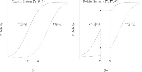
Theorem 2.3 shows that the redundant portions in a toxicity system can be removed so that a simpler system can be considered. The following corollary is a direct result from Theorem 2.3.

Corollary 2.1

Suppose Y is a continuous toxicity response which takes value on interval $\mathbb{Y}=[a,b]$, where $-\mathrm{\infty }<a<b<+\mathrm{\infty }$ and $(\mathbb{Y},\mathit{F},\theta )$ is a toxicity system. If the target toxicity probability $\theta =\theta \left(y\right)$ is a stepwise increasing function, i.e., there exists ${\theta }_1>\cdots >{\theta }_M$ such that $\theta =\theta \left(y\right)=\left\{\begin{array}{ll}{\theta }_1,& \text{if }a\le y<y_1,\\ {\theta }_2,& \text{if }{y}_1\le y<y_2,\\ ⋮& ⋮\\ {\theta }_M,& \text{if {}{y}_{M-1}\le y\le b\text{},}\end{array}\right.$then the toxicity system $(\mathbb{Y},\mathit{F},\theta )$ reduces to a polychotomous toxicity system $({\mathbb{Y}}^{\ast },{\mathit{F}}^{\ast },{\theta }^{\ast })$, where ${\mathbb{Y}}^{\ast }=\{1,\dots ,M\}$ which is a polychotomization of $\mathbb{Y}$ corresponding to the bin boundaries $a=y_0<y_1<\cdots <y_{M-1}<y_M=b$, and ${\theta }^{\ast }=\{{\theta }_1,\dots {\theta }_M\}$. Furthermore, ${\mathit{F}}^{\ast }=\left\{F^{\ast }\right(y|x),-\mathrm{\infty }<y<\mathrm{\infty }|x\in \mathbb{X}\}$ such that, $\begin{array}{rl}& F^{\ast }\left(y|x\right)\\ & =\left\{\begin{array}{ll}0,& \text{if }y<a,\\ F\left(y_i|x\right),& \text{if }{y}_{i-1}\le y<y_i,\text{ for }i=1,\dots ,M,\\ 1,& \text{if }y\ge b,\end{array}\right.\end{array}$where $F(\cdot |x)\in \mathit{F}$, for all $x\in \mathbb{X}$.

Corollary 2.1 shows that once the target toxicity tolerance probability curve is reduced to a step function, we reduce the continuous toxicity response problem to a polychotomous toxicity response problem.

3. Continuous toxicity response case: location and scale family response with linear mean in dose x

Suppose that a continuous toxicity response Y belongs to a location-scale family with the cumulative distribution function (5) $Y|x\sim F\left(\frac{y-({\text{β}}_0+{\text{β}}_{1}x)}{\sigma }\right),-\mathrm{\infty }<y<\mathrm{\infty },$(5) at dose level x, where ${\text{β}}_1>0$. In order to obtain an analytic solution of the overall MTD, a common scale parameter, σ, is assumed and the location parameter, $\mu \left(x\right)={\text{β}}_0+{\text{β}}_{1}x$, is assumed to be linearly increasing in the dose level x.

In practice, it is common to give a lower critical value, $y_0$, and a upper critical value, $y_1$, for the toxicity grade $\mathbb{Y}$. Only those toxicity grades which fall in interval $(y_0,y_1)$ are seriously considered. Hence, based on Theorem 2.3, one can define the target toxicity tolerance probability as follows. (6) $\theta =\theta \left(y\right)=\left\{\begin{array}{ll}1,& \text{if }y\le y_0,\\ h(y,y_0,y_1),& \text{if }{y}_0<y<y_1,\\ {\theta }_0,& \text{if }y\ge y_1,\end{array}\right.,$(6) where $0<{\theta }_0\le h(y,y_0,y_1)\le 1$ for all $y\in (y_0,y_1)$ and $h(y,y_0,y_1)$ is strictly decreasing in y. Usually, ${\theta }_0=0$ means the toxicity is 100% fatal and hence we can restrict to ${\theta }_0>0$, since extremely large toxic grades should be avoided as much as possible.

Since ${\text{β}}_1>0$ due to the fact the probability of the toxicity increases in dosage, according to (2(2) $\begin{array}{rl}{}_y\mathrm{M}\mathrm{T}\mathrm{D}\left(\theta \right)& =sup\left\{x|P\right(Y\ge y|x)\le \theta \}\\ & =sup\left\{x|P\right(Y<y|x)\ge 1-\theta \}.\end{array}$(2) ), the level-y MTD is (7) $\begin{array}{rl}& {}_y\mathrm{M}\mathrm{T}\mathrm{D}\left(h\right(y,y_0,y_1\left)\right)\\ & =\left\{\begin{array}{ll}\mathrm{\infty },y-\sigma F^{-1}[1-& \text{for }y\le y_0,\\ \frac{h(y,y_0,y_1)]-{\text{β}}_0}{{\text{β}}_1},& \text{for }y\in (y_0,y_1),\\ \frac{y-\sigma F^{-1}(1-{\theta }_0)-{\text{β}}_0}{{\text{β}}_1},& \text{for }y\ge y_1.\end{array}\right.\end{array}$(7) Consequently, since ${\text{β}}_1>0$ the overall MTD is (8) $\begin{array}{rl}{}^{\mathbb{Y}}\mathrm{M}\mathrm{T}\mathrm{D}\left(\theta \right)& =\underset{y\in \mathbb{Y}}{inf}\left\{{}_y\mathrm{M}\mathrm{T}\mathrm{D}\right(\theta \left(y\right)\left)\right\}\\ & =min\left\{\underset{y\le y_0}{inf}\left\{{}_y\mathrm{M}\mathrm{T}\mathrm{D}\right(\theta \left(y\right)\left)\right\},\right.\\ & \underset{y\in (y_0,y_1)}{inf}\left\{{}_y\mathrm{M}\mathrm{T}\mathrm{D}\right(\theta \left(y\right)\left)\right\},\\ & \left.\underset{y\ge y_1}{inf}\left\{{}_y\mathrm{M}\mathrm{T}\mathrm{D}\right(\theta \left(y\right)\left)\right\}\right\}\\ & =min\{x_1^{\ast },x_2^{\ast }\},\end{array}$(8) where, $\begin{array}{rl}{x}_1^{\ast }& =\underset{y\in (y_0,y_1)}{inf}\left\{\frac{y-\sigma F^{-1}[1-h(y,y_0,y_1\left)\right]-{\text{β}}_0}{{\text{β}}_1}\right\},\end{array}$ and $\begin{array}{rl}{x}_2^{\ast }& =\frac{y_1-\sigma F^{-1}(1-{\theta }_0)-{\text{β}}_0}{{\text{β}}_1}.\end{array}$Since $({\text{β}}_0,{\text{β}}_1)$ are constants, we have $\begin{array}{rl}& \mathrm{a}\mathrm{r}\mathrm{g}inf\left\{\frac{y-\sigma F^{-1}[1-h(y,y_0,y_1\left)\right]-{\text{β}}_0}{{\text{β}}_1}\right\}\\ & =\mathrm{a}\mathrm{r}\mathrm{g}inf\{y-\sigma F^{-1}[1-h(y,y_0,y_1)\left]\right\}.\end{array}$Hence, for a fixed distribution $F(\cdot )$, the optimal point, $y^{\ast }$, is only determined by the target toxicity tolerance probability $h(y,y_0,y_1)$. Therefore, the choice of the function $h(y,y_0,y_1)$ in (6(6) $\theta =\theta \left(y\right)=\left\{\begin{array}{ll}1,& \text{if }y\le y_0,\\ h(y,y_0,y_1),& \text{if }{y}_0<y<y_1,\\ {\theta }_0,& \text{if }y\ge y_1,\end{array}\right.,$(6) ) is crucial. In Example 3.1 with the normal response, we will discuss the choice of $h(y,y_0,y_1)$. According to (7(7) $\begin{array}{rl}& {}_y\mathrm{M}\mathrm{T}\mathrm{D}\left(h\right(y,y_0,y_1\left)\right)\\ & =\left\{\begin{array}{ll}\mathrm{\infty },y-\sigma F^{-1}[1-& \text{for }y\le y_0,\\ \frac{h(y,y_0,y_1)]-{\text{β}}_0}{{\text{β}}_1},& \text{for }y\in (y_0,y_1),\\ \frac{y-\sigma F^{-1}(1-{\theta }_0)-{\text{β}}_0}{{\text{β}}_1},& \text{for }y\ge y_1.\end{array}\right.\end{array}$(7) ), the following propositions are straightforward.

Proposition 3.1

Suppose $F(\cdot )$ is the standard cumulative distribution function of the location-scale family in (5(5) $Y|x\sim F\left(\frac{y-({\text{β}}_0+{\text{β}}_{1}x)}{\sigma }\right),-\mathrm{\infty }<y<\mathrm{\infty },$(5) ) and the target toxicity tolerance probability is in the form of (6(6) $\theta =\theta \left(y\right)=\left\{\begin{array}{ll}1,& \text{if }y\le y_0,\\ h(y,y_0,y_1),& \text{if }{y}_0<y<y_1,\\ {\theta }_0,& \text{if }y\ge y_1,\end{array}\right.,$(6) ). Then, for a fixed ${\text{β}}_1>0$, the overall MTD is decreasing in ${\text{β}}_0$.

Proposition 3.1 indicates that, for a fixed positive slope ${\text{β}}_1$, the higher the mean toxicity response of a toxicity system, the lower is the overall MTD.

Proposition 3.2

Suppose $F(\cdot )$ is the standard cumulative distribution function of the location-scale family in (5(5) $Y|x\sim F\left(\frac{y-({\text{β}}_0+{\text{β}}_{1}x)}{\sigma }\right),-\mathrm{\infty }<y<\mathrm{\infty },$(5) ) and the target toxicity tolerance probability is in the form of (6(6) $\theta =\theta \left(y\right)=\left\{\begin{array}{ll}1,& \text{if }y\le y_0,\\ h(y,y_0,y_1),& \text{if }{y}_0<y<y_1,\\ {\theta }_0,& \text{if }y\ge y_1,\end{array}\right.,$(6) ). Then, for fixed ${\text{β}}_0$,

(a)	if $y^{\ast }-\sigma F^{-1}[1-h(y^{\ast },y_0,y_1\left)\right]<{\text{β}}_0$, the overall MTD is increasing in ${\text{β}}_1$;
(b)	if $y^{\ast }-\sigma F^{-1}[1-h(y^{\ast },y_0,y_1\left)\right]>{\text{β}}_0$, the overall MTD is decreasing in ${\text{β}}_1$,

where $y^{\ast }=\mathrm{a}\mathrm{r}\mathrm{g}inf\{y-\sigma F^{-1}[1-h(y,y_0,y_1)\left]\right\}$.

Next, we use normal toxicity response with linear predictor (dose) to illustrate the location-scale family responses.

Example 3.1

Normal Response

Suppose that the continuous toxicity response Y has a cumulative distribution function (9) $Y|x\sim \mathrm{\Phi }\left(\frac{y-({\text{β}}_0+{\text{β}}_{1}x)}{\sigma }\right),-\mathrm{\infty }<y<\mathrm{\infty },$(9) at dose level x, where ${\text{β}}_1>0$, and $\mathrm{\Phi }(\cdot )$ is the cumulative distribution function of the standard normal random variable.

In order to illustrate the proposed dose-finding strategy for the continuous toxicity response, we choose the following target toxicity tolerance probability function (10) $\begin{array}{rl}{\theta }_{\alpha }& ={\theta }_{\alpha }\left(y\right)\\ & =\left\{\begin{array}{ll}1,& \mathrm{i}\mathrm{f}y\le y_0,\\ {\theta }_0+(1-{\theta }_0){\left(\frac{y_1-y}{y_1-y_0}\right)}^{\alpha },& \mathrm{i}\mathrm{f}{y}_0<y<y_1,\\ {\theta }_0,& \mathrm{i}\mathrm{f}y\ge y_1,\end{array}\right.\end{array}$(10) where $\alpha >0$. It is easy to verify that (10(10) $\begin{array}{rl}{\theta }_{\alpha }& ={\theta }_{\alpha }\left(y\right)\\ & =\left\{\begin{array}{ll}1,& \mathrm{i}\mathrm{f}y\le y_0,\\ {\theta }_0+(1-{\theta }_0){\left(\frac{y_1-y}{y_1-y_0}\right)}^{\alpha },& \mathrm{i}\mathrm{f}{y}_0<y<y_1,\\ {\theta }_0,& \mathrm{i}\mathrm{f}y\ge y_1,\end{array}\right.\end{array}$(10) ) is a special case of (6(6) $\theta =\theta \left(y\right)=\left\{\begin{array}{ll}1,& \text{if }y\le y_0,\\ h(y,y_0,y_1),& \text{if }{y}_0<y<y_1,\\ {\theta }_0,& \text{if }y\ge y_1,\end{array}\right.,$(6) ).

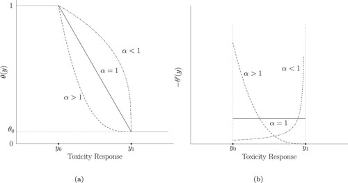
Figure 3(a) shows the target toxicity tolerance probability curve of $\theta \left(y\right)$ in (10(10) $\begin{array}{rl}{\theta }_{\alpha }& ={\theta }_{\alpha }\left(y\right)\\ & =\left\{\begin{array}{ll}1,& \mathrm{i}\mathrm{f}y\le y_0,\\ {\theta }_0+(1-{\theta }_0){\left(\frac{y_1-y}{y_1-y_0}\right)}^{\alpha },& \mathrm{i}\mathrm{f}{y}_0<y<y_1,\\ {\theta }_0,& \mathrm{i}\mathrm{f}y\ge y_1,\end{array}\right.\end{array}$(10) ). On interval $(y_0,y_1)$, $\theta \left(y\right)$ is convex if the power $\alpha >1$, concave if the power $\alpha <1$ and straightly decreasing if the power $\alpha =1$. Figure 3(b) shows the negative derivative curve of the $\theta \left(y\right)$. It is clear that if $\alpha >1$, the toxicity tolerance probability decreases quickly as the toxicity response level increases near the lower toxicity response level which means that the drug in study could quickly become toxic in the range. On the other hand, if $\alpha <1$, the toxicity tolerance probability decreases slowly as the toxicity response level increases near the lower toxicity response level and then moves quickly near the upper toxicity response level. If $\alpha =1$, the toxicity tolerance probability from $y_0$ to $y_1$ decreases at the same rate. In Section 4, simulation studies are preformed to check the influence of the power α on the overall MTD.

Figure 3. Graph illustration for (a) the target toxicity tolerance probability with form (10(10) $\begin{array}{rl}{\theta }_{\alpha }& ={\theta }_{\alpha }\left(y\right)\\ & =\left\{\begin{array}{ll}1,& \mathrm{i}\mathrm{f}y\le y_0,\\ {\theta }_0+(1-{\theta }_0){\left(\frac{y_1-y}{y_1-y_0}\right)}^{\alpha },& \mathrm{i}\mathrm{f}{y}_0<y<y_1,\\ {\theta }_0,& \mathrm{i}\mathrm{f}y\ge y_1,\end{array}\right.\end{array}$(10) ) and (b) the negative derivative curve of the target toxicity tolerance probability.

Under this setting, both $\mathrm{\Phi }(\cdot )$ and $\theta (\cdot )$ are continuous functions. Hence, using (8(8) $\begin{array}{rl}{}^{\mathbb{Y}}\mathrm{M}\mathrm{T}\mathrm{D}\left(\theta \right)& =\underset{y\in \mathbb{Y}}{inf}\left\{{}_y\mathrm{M}\mathrm{T}\mathrm{D}\right(\theta \left(y\right)\left)\right\}\\ & =min\left\{\underset{y\le y_0}{inf}\left\{{}_y\mathrm{M}\mathrm{T}\mathrm{D}\right(\theta \left(y\right)\left)\right\},\right.\\ & \underset{y\in (y_0,y_1)}{inf}\left\{{}_y\mathrm{M}\mathrm{T}\mathrm{D}\right(\theta \left(y\right)\left)\right\},\\ & \left.\underset{y\ge y_1}{inf}\left\{{}_y\mathrm{M}\mathrm{T}\mathrm{D}\right(\theta \left(y\right)\left)\right\}\right\}\\ & =min\{x_1^{\ast },x_2^{\ast }\},\end{array}$(8) ), the overall MTD under this setting is (11) $\begin{array}{r}{}^{\mathbb{Y}}\mathrm{M}\mathrm{T}\mathrm{D}\left({\theta }_{\alpha }\right)=\underset{y\in (y_0,y_1)}{inf}\left\{\begin{array}{c}y-\sigma {\mathrm{\Phi }}^{-1}\left\{\right(1-{\theta }_0)\\ \times [1-(\frac{y_1-y}{y_1-y_0}{)}^{\alpha }\left]\right\}-{\text{β}}_0\end{array}\right\}{\text{β}}_1^{-1}.\end{array}$(11) Based on (11(11) $\begin{array}{r}{}^{\mathbb{Y}}\mathrm{M}\mathrm{T}\mathrm{D}\left({\theta }_{\alpha }\right)=\underset{y\in (y_0,y_1)}{inf}\left\{\begin{array}{c}y-\sigma {\mathrm{\Phi }}^{-1}\left\{\right(1-{\theta }_0)\\ \times [1-(\frac{y_1-y}{y_1-y_0}{)}^{\alpha }\left]\right\}-{\text{β}}_0\end{array}\right\}{\text{β}}_1^{-1}.\end{array}$(11) ), the following proposition is proven in the Appendix.

Proposition 3.3

Suppose that the toxicity response is normally distributed as in (9(9) $Y|x\sim \mathrm{\Phi }\left(\frac{y-({\text{β}}_0+{\text{β}}_{1}x)}{\sigma }\right),-\mathrm{\infty }<y<\mathrm{\infty },$(9) ), and the target toxicity tolerance probability is set to be of the form (10(10) $\begin{array}{rl}{\theta }_{\alpha }& ={\theta }_{\alpha }\left(y\right)\\ & =\left\{\begin{array}{ll}1,& \mathrm{i}\mathrm{f}y\le y_0,\\ {\theta }_0+(1-{\theta }_0){\left(\frac{y_1-y}{y_1-y_0}\right)}^{\alpha },& \mathrm{i}\mathrm{f}{y}_0<y<y_1,\\ {\theta }_0,& \mathrm{i}\mathrm{f}y\ge y_1,\end{array}\right.\end{array}$(10) ), then the overall MTD in (11(11) $\begin{array}{r}{}^{\mathbb{Y}}\mathrm{M}\mathrm{T}\mathrm{D}\left({\theta }_{\alpha }\right)=\underset{y\in (y_0,y_1)}{inf}\left\{\begin{array}{c}y-\sigma {\mathrm{\Phi }}^{-1}\left\{\right(1-{\theta }_0)\\ \times [1-(\frac{y_1-y}{y_1-y_0}{)}^{\alpha }\left]\right\}-{\text{β}}_0\end{array}\right\}{\text{β}}_1^{-1}.\end{array}$(11) ) is decreasing in α and (12) $\begin{array}{rl}\underset{\alpha \to \mathrm{\infty }}{lim}{}^{\mathbb{Y}}\mathrm{M}\mathrm{T}\mathrm{D}\left({\theta }_{\alpha }\right)& =\frac{y_0-\sigma {\mathrm{\Phi }}^{-1}(1-{\theta }_0)-{\text{β}}_0}{{\text{β}}_1}\\ & =\frac{y_0+\sigma {\mathrm{\Phi }}^{-1}\left({\theta }_0\right)-{\text{β}}_0}{{\text{β}}_1},\end{array}$(12) where ${}^{\mathbb{Y}}\mathrm{M}\mathrm{T}\mathrm{D}\left({\theta }_{\alpha }\right)$ is defined in (11(11) $\begin{array}{r}{}^{\mathbb{Y}}\mathrm{M}\mathrm{T}\mathrm{D}\left({\theta }_{\alpha }\right)=\underset{y\in (y_0,y_1)}{inf}\left\{\begin{array}{c}y-\sigma {\mathrm{\Phi }}^{-1}\left\{\right(1-{\theta }_0)\\ \times [1-(\frac{y_1-y}{y_1-y_0}{)}^{\alpha }\left]\right\}-{\text{β}}_0\end{array}\right\}{\text{β}}_1^{-1}.\end{array}$(11) ).

Proposition 3.3 shows that the larger the power α is or the more expected weights the lower toxicity response (close to left critical point $y_0$) is assigned, the lower the overall MTD is. As the power $\alpha \to \mathrm{\infty }$, the minimum overall MTD is obtained at the dose level $x^{\ast }$ at which the probability of level-$y_0$ severe toxicity $T_{y_0}=\{Y\ge y_0\}$ achieves ${\theta }_0$, i.e., $P(Y\ge y_0|x^{\ast })={\theta }_0$.

Notice that as $\alpha \to \mathrm{\infty }$, the target toxicity probability in (10(10) $\begin{array}{rl}{\theta }_{\alpha }& ={\theta }_{\alpha }\left(y\right)\\ & =\left\{\begin{array}{ll}1,& \mathrm{i}\mathrm{f}y\le y_0,\\ {\theta }_0+(1-{\theta }_0){\left(\frac{y_1-y}{y_1-y_0}\right)}^{\alpha },& \mathrm{i}\mathrm{f}{y}_0<y<y_1,\\ {\theta }_0,& \mathrm{i}\mathrm{f}y\ge y_1,\end{array}\right.\end{array}$(10) ) reduces to ${\theta }_{\alpha }={\theta }_{\alpha }\left(y\right)=\left\{\begin{array}{ll}1,& \mathrm{i}\mathrm{f}y\le y_0,\\ {\theta }_0,& \mathrm{i}\mathrm{f}y>y_0.\end{array}\right.$According to Corollary 2.1, the continuous toxicity system reduces to the dichotomous toxicity system shown in Section 2.2. The MTD can thus be determined as (13) $\mathrm{M}\mathrm{T}\mathrm{D}=\frac{{\mathrm{\Phi }}^{-1}\left({\theta }_0\right)-{\text{β}}_0^{\ast }}{{\text{β}}_1}.$(13) In (12(12) $\begin{array}{rl}\underset{\alpha \to \mathrm{\infty }}{lim}{}^{\mathbb{Y}}\mathrm{M}\mathrm{T}\mathrm{D}\left({\theta }_{\alpha }\right)& =\frac{y_0-\sigma {\mathrm{\Phi }}^{-1}(1-{\theta }_0)-{\text{β}}_0}{{\text{β}}_1}\\ & =\frac{y_0+\sigma {\mathrm{\Phi }}^{-1}\left({\theta }_0\right)-{\text{β}}_0}{{\text{β}}_1},\end{array}$(12) ), denote ${\text{β}}_0^{\ast }={\text{β}}_0-y_0$ and set $\sigma =1$, then (13(13) $\mathrm{M}\mathrm{T}\mathrm{D}=\frac{{\mathrm{\Phi }}^{-1}\left({\theta }_0\right)-{\text{β}}_0^{\ast }}{{\text{β}}_1}.$(13) ) and (12(12) $\begin{array}{rl}\underset{\alpha \to \mathrm{\infty }}{lim}{}^{\mathbb{Y}}\mathrm{M}\mathrm{T}\mathrm{D}\left({\theta }_{\alpha }\right)& =\frac{y_0-\sigma {\mathrm{\Phi }}^{-1}(1-{\theta }_0)-{\text{β}}_0}{{\text{β}}_1}\\ & =\frac{y_0+\sigma {\mathrm{\Phi }}^{-1}\left({\theta }_0\right)-{\text{β}}_0}{{\text{β}}_1},\end{array}$(12) ) are exactly same. In the dichotomous case discussed in Yang et al. (2010), the underlying distribution of the toxicity response is unknown, hence we introduce the normal latent variable. In this study, the toxicity response is assumed to be normally distributed. Hence, (12(12) $\begin{array}{rl}\underset{\alpha \to \mathrm{\infty }}{lim}{}^{\mathbb{Y}}\mathrm{M}\mathrm{T}\mathrm{D}\left({\theta }_{\alpha }\right)& =\frac{y_0-\sigma {\mathrm{\Phi }}^{-1}(1-{\theta }_0)-{\text{β}}_0}{{\text{β}}_1}\\ & =\frac{y_0+\sigma {\mathrm{\Phi }}^{-1}\left({\theta }_0\right)-{\text{β}}_0}{{\text{β}}_1},\end{array}$(12) ) is obtained as the power α in (10(10) $\begin{array}{rl}{\theta }_{\alpha }& ={\theta }_{\alpha }\left(y\right)\\ & =\left\{\begin{array}{ll}1,& \mathrm{i}\mathrm{f}y\le y_0,\\ {\theta }_0+(1-{\theta }_0){\left(\frac{y_1-y}{y_1-y_0}\right)}^{\alpha },& \mathrm{i}\mathrm{f}{y}_0<y<y_1,\\ {\theta }_0,& \mathrm{i}\mathrm{f}y\ge y_1,\end{array}\right.\end{array}$(10) ) goes to infinity. Table 1 shows illustrative results of MTD in Proposition 3.3 for various α.

Table 1. An Illustration of Proposition 3.3. The parameters for the true model are ${\text{β}}_0=-1$, ${\text{β}}_1=1$ and $\sigma =1$. The parameters for the target toxicity tolerance probability are $y_0=-1$, $y_1=1$ and ${\theta }_0=0.05$.

α	$y^{\ast }$	MTD(${\theta }_{\alpha }$)	α	$y^{\ast }$	MTD(${\theta }_{\alpha }$)
1	1.00	0.35	10	−0.34	−0.84
2	0.72	0.23	50	−0.79	−1.40
3	0.34	−0.04	100	−0.88	−1.51
4	0.14	−0.25	1000	−0.98	−1.63
5	0.00	−0.41	10000	−1.00	−1.64

4. Simulation studies for the normal toxicity response with Bayesian analysis

4.1. Bayesian posterior analysis

Suppose $d_1,\dots ,d_K$ are K ordered dose levels under investigation. Let ${\mathcal{F}}_j=\left\{\right(x_1,y_1),\dots ,(x_j,y_j\left)\right\}$denote the history of the first j assignments and responses, where $x_l\in \{d_1,\dots ,d_K\}$ is the dose level assigned to the lth patient and $y_l$ is the corresponding observed response, $l=1,\dots ,j$. According to (9(9) $Y|x\sim \mathrm{\Phi }\left(\frac{y-({\text{β}}_0+{\text{β}}_{1}x)}{\sigma }\right),-\mathrm{\infty }<y<\mathrm{\infty },$(9) ) in Example 3.1, the likelihood function of ${\text{β}}_0$, ${\text{β}}_1$ and ${\sigma }^2$ is $\begin{array}{rl}& L({\text{β}}_0,{\text{β}}_1,{\sigma }^2|{\mathcal{F}}_j)\\ & =\prod _{l=1}^j\frac{1}{\sqrt{2\pi {\sigma }^2}}\\ & \times \exp \left\{-\frac{[y_l-({\text{β}}_0+{\text{β}}_1{x}_l){]}^2}{2{\sigma }^2}\right\}\\ & \propto ({\sigma }^2{)}^{-j/2}\exp \left\{-\frac{1}{2{\sigma }^2}\sum _{l=1}^j[y_l-{\text{β}}_0-{\text{β}}_1{x}_l{]}^2\right\}.\end{array}$Let $\pi ({\text{β}}_0,{\text{β}}_1,{\sigma }^2)$ be the prior on $({\text{β}}_0,{\text{β}}_1,{\sigma }^2)$, the joint posterior density function of $({\text{β}}_0,{\text{β}}_1,{\sigma }^2)$ given data ${\mathcal{F}}_j$ is (14) $\begin{array}{rl}& \pi ({\text{β}}_0,{\text{β}}_1,{\sigma }^2|{\mathcal{F}}_j)\propto \pi ({\text{β}}_0,{\text{β}}_1,{\sigma }^2)({\sigma }^2{)}^{-j/2}\\ & \times \exp \left\{-\frac{1}{2{\sigma }^2}\sum _{l=1}^j[y_l-{\text{β}}_0-{\text{β}}_1{x}_l{]}^2\right\}.\end{array}$(14) Since it is assumed that the average toxicity response is increasing in dose level x, i.e., the parameter ${\text{β}}_1$ is assumed to be greater than 0, the prior $\pi ({\text{β}}_0,{\text{β}}_1,{\sigma }^2)$ should be defined on $\left\{\right({\text{β}}_0,{\text{β}}_1,{\sigma }^2)|{\text{β}}_1>0,{\sigma }^2>0\}$. Furthermore, we assume that $({\text{β}}_0,{\text{β}}_1,{\sigma }^2)$ are independent in the prior. According to (14(14) $\begin{array}{rl}& \pi ({\text{β}}_0,{\text{β}}_1,{\sigma }^2|{\mathcal{F}}_j)\propto \pi ({\text{β}}_0,{\text{β}}_1,{\sigma }^2)({\sigma }^2{)}^{-j/2}\\ & \times \exp \left\{-\frac{1}{2{\sigma }^2}\sum _{l=1}^j[y_l-{\text{β}}_0-{\text{β}}_1{x}_l{]}^2\right\}.\end{array}$(14) ), the full conditional posterior distributions are obtained as follows.

$\pi ({\text{β}}_0|{\text{β}}_1,{\sigma }^2,{\mathcal{F}}_j)$: The posterior densities of ${\text{β}}_0$, given ${\text{β}}_1$, ${\sigma }^2$ and data, is given as follows.

• If a flat prior $\pi \left({\text{β}}_0\right)\propto 1$ is assigned on ${\text{β}}_0$, then, ${\text{β}}_0|{\text{β}}_1,{\sigma }^2,{\mathcal{F}}_j\sim N\left(\frac{\sum _{l=1}^j(y_l-{\text{β}}_1{x}_l)}{j},\frac{{\sigma }^2}{j}\right).$

• If a proper conjugate prior $N({\overline{\text{β}}}_0,{\overline{\sigma }}_0^2)$ is assigned, then, $\begin{array}{rl}& {\text{β}}_0|{\text{β}}_1,{\sigma }^2,{\mathcal{F}}_j\\ & \sim N\left(\frac{{\overline{\sigma }}_0^2\sum _{l=1}^j(z_l-{\text{β}}_1{x}_l)+{\sigma }^2{\overline{\text{β}}}_0}{{\sigma }^2+{\overline{\sigma }}_0^{2}j},\frac{{\sigma }^2{\overline{\sigma }}_0^2}{{\sigma }^2+{\overline{\sigma }}_0^{2}j}\right).\end{array}$

$\pi ({\text{β}}_1|{\text{β}}_0,{\sigma }^2,{\mathcal{F}}_j)$: The posterior densities of ${\text{β}}_1$, given ${\text{β}}_0$, ${\sigma }^2$ and data, is given as follows.

• If a flat prior $\pi \left({\text{β}}_1\right)\propto I({\text{β}}_1>0)$ is assigned on ${\text{β}}_1$, then, $\begin{array}{rl}& {\text{β}}_1|{\text{β}}_0,{\sigma }^2,{\mathcal{F}}_j\\ & \sim N\left(\frac{\sum _{l=1}^j(y_l-{\text{β}}_0)x_l}{\sum _{l=1}^j{x}_l^2},\frac{{\sigma }^2}{\sum _{l=1}^j{x}_l^2}\right)I({\text{β}}_1>0).\end{array}$

• If a proper conjugate truncated normal prior $N({\overline{\text{β}}}_1,{\overline{\sigma }}_1^2)I({\text{β}}_1>0)$ is assigned, then, $\begin{array}{rl}{\text{β}}_1|{\text{β}}_0,{\sigma }^2,{\mathcal{F}}_j& \sim N\left(\frac{{\overline{\sigma }}_1^2\sum _{l=1}^j(y_l-{\text{β}}_0)x_l+{\sigma }^2{\overline{\text{β}}}_1}{{\sigma }^2+{\overline{\sigma }}_1^2\sum _{l=1}^j{x}_l^2},\right.\\ & \left.\frac{{\sigma }^2{\overline{\sigma }}_1^2}{{\sigma }^2+{\overline{\sigma }}_1^2\sum _{l=1}^j{x}_l^2}\right)I({\text{β}}_1>0).\end{array}$

• If a proper, but non-conjugate exponential prior $\exp \{-{\text{β}}_1\}I({\text{β}}_1>0)$ is assigned, then, $\begin{array}{rl}{\text{β}}_1|{\text{β}}_0,{\sigma }^2,{\mathcal{F}}_j& \sim N\left(\frac{\sum _{l=1}^j(y_l-{\text{β}}_0)x_l-{\sigma }^2}{\sum _{l=1}^j{x}_l^2},\right.\\ & \left.\frac{{\sigma }^2}{\sum _{l=1}^j{x}_l^2}\right)I({\text{β}}_1>0).\end{array}$

$\pi ({\sigma }^2|{\text{β}}_0,{\text{β}}_1,{\mathcal{F}}_j)$: The posterior densities of ${\sigma }^2$, given ${\text{β}}_0$, ${\text{β}}_2$ and data, is given as follows.

• If ${\sigma }^2$ has an inverse gamma prior $\mathrm{I}\mathrm{n}\mathrm{v}-\mathrm{G}\mathrm{a}\mathrm{m}\mathrm{m}\mathrm{a}(a,b)$ with the probability density function. Then the posterior distribution of ${\sigma }^2$, given ${\text{β}}_0$ and ${\text{β}}_1$, follows $\begin{array}{rl}{\sigma }^2|{\text{β}}_0,{\text{β}}_1,{\mathcal{F}}_j& \sim \mathrm{I}\mathrm{n}\mathrm{v}-\mathrm{G}\mathrm{a}\mathrm{m}\mathrm{m}\mathrm{a}\left(\phantom{\sum _{l=1}^j}a+j/2,b\right.\\ & +\left.\sum _{l=1}^j(y_l-{\text{β}}_0-{\text{β}}_1{x}_l{)}^2/2\right).\end{array}$

• If $\pi \left({\sigma }^2\right)\propto 1/{\sigma }^2$, then $\begin{array}{rl}& {\sigma }^2|{\text{β}}_0,{\text{β}}_1,{\mathcal{F}}_j\\ & \sim \mathrm{I}\mathrm{n}\mathrm{v}-\mathrm{G}\mathrm{a}\mathrm{m}\mathrm{m}\mathrm{a}\left(j/2,\sum _{l=1}^j(y_l-{\text{β}}_0-{\text{β}}_1{x}_l{)}^2/2\right).\end{array}$

4.2. MTD determination procedure

Based on the Gibbs samplers, ${\text{β}}_0,{\text{β}}_1$, and ${\sigma }^2$ could be generated from those full conditional posterior distributions given in Section 4.1. After drawing from the joint posterior distribution $\pi ({\text{β}}_0,{\text{β}}_1,{\sigma }^2|{\mathcal{F}}_j)$, one can estimate the overall MTD by using the following formula. (15) $\begin{array}{rl}& {}^{\mathbb{Y}}\widehat{\mathrm{M}\mathrm{T}\mathrm{D}}\left({\theta }_{\alpha }\right)\\ & =\underset{y\in (y_0,y_1)}{inf}\left\{\begin{array}{c}y-\hat{\sigma }{\mathrm{\Phi }}^{-1}\left\{\right(1-{\theta }_0)\\ \times [1-(\frac{y_1-y}{y_1-y_0}{)}^{\alpha }\left]\right\}-\widehat{{\text{β}}_0}\end{array}\right\}{\widehat{\text{β}}}_1^{-1}.\end{array}$(15) The estimates of the parameters in (15(15) $\begin{array}{rl}& {}^{\mathbb{Y}}\widehat{\mathrm{M}\mathrm{T}\mathrm{D}}\left({\theta }_{\alpha }\right)\\ & =\underset{y\in (y_0,y_1)}{inf}\left\{\begin{array}{c}y-\hat{\sigma }{\mathrm{\Phi }}^{-1}\left\{\right(1-{\theta }_0)\\ \times [1-(\frac{y_1-y}{y_1-y_0}{)}^{\alpha }\left]\right\}-\widehat{{\text{β}}_0}\end{array}\right\}{\widehat{\text{β}}}_1^{-1}.\end{array}$(15) ) can be obtained based on the MCMC simulation. Suppose one has obtained N generations of $({\text{β}}_0,{\text{β}}_1,{\sigma }^2)$, which are $({\text{β}}_0^{\left(i\right)},{\text{β}}_1^{\left(i\right)},({\sigma }^2{)}^{\left(i\right)}),i=1,2,\dots ,N$, then, $\begin{array}{rl}\widehat{{\text{β}}_0}& ={\hat{E}}^{\pi \left({\text{β}}_0|{\mathcal{F}}_j\right)}\left({\text{β}}_0\right)=\frac{1}{N}\sum _{i=1}^N{\text{β}}_0^{\left(i\right)},\\ \widehat{{\text{β}}_1}& ={\hat{E}}^{\pi \left({\text{β}}_1|{\mathcal{F}}_j\right)}\left({\text{β}}_1\right)=\frac{1}{N}\sum _{i=1}^N{\text{β}}_1^{\left(i\right)},\end{array}$ and $\begin{array}{rl}\hat{\sigma }& =\sqrt{{\hat{E}}^{\pi \left({\sigma }^2|{\mathcal{F}}_j\right)}\left({\sigma }^2\right)}=\sqrt{\frac{1}{N}\sum _{i=1}^N({\sigma }^2{)}^{\left(i\right)}}.\end{array}$With regarding to the dose allocation, one can find the next dose level $x_{j+1}\in \{d_1,\dots ,d_K\}$, at which the $(j+1)$th patient is to be treated, such that it is the closest dose to the estimated overall MTD, i.e., (16) $x_{j+1}=\underset{x\in \{d_1,\dots ,d_K\}}{\mathrm{a}\mathrm{r}\mathrm{g}\mathrm{m}\mathrm{i}\mathrm{n}}\left\{|x{-}^{\mathbb{Y}}\widehat{\mathrm{M}\mathrm{T}\mathrm{D}}\right({\theta }_{\alpha }\left)|\right\},$(16) where ${}^{\mathbb{Y}}\widehat{\mathrm{M}\mathrm{T}\mathrm{D}}\left({\theta }_{\alpha }\right)$ is obtained from (15(15) $\begin{array}{rl}& {}^{\mathbb{Y}}\widehat{\mathrm{M}\mathrm{T}\mathrm{D}}\left({\theta }_{\alpha }\right)\\ & =\underset{y\in (y_0,y_1)}{inf}\left\{\begin{array}{c}y-\hat{\sigma }{\mathrm{\Phi }}^{-1}\left\{\right(1-{\theta }_0)\\ \times [1-(\frac{y_1-y}{y_1-y_0}{)}^{\alpha }\left]\right\}-\widehat{{\text{β}}_0}\end{array}\right\}{\widehat{\text{β}}}_1^{-1}.\end{array}$(15) ). After collecting the $(j+1)$th response $y_{j+1}$, given ${\mathcal{F}}_{j+1}=\left\{\right(x_1,y_1),\dots ,(x_j,y_j),(x_{j+1},y_{j+1}\left)\right\}$, the updated overall MTD can be obtained from (15(15) $\begin{array}{rl}& {}^{\mathbb{Y}}\widehat{\mathrm{M}\mathrm{T}\mathrm{D}}\left({\theta }_{\alpha }\right)\\ & =\underset{y\in (y_0,y_1)}{inf}\left\{\begin{array}{c}y-\hat{\sigma }{\mathrm{\Phi }}^{-1}\left\{\right(1-{\theta }_0)\\ \times [1-(\frac{y_1-y}{y_1-y_0}{)}^{\alpha }\left]\right\}-\widehat{{\text{β}}_0}\end{array}\right\}{\widehat{\text{β}}}_1^{-1}.\end{array}$(15) ). Continue in this way until the results of the last patient, say nth, are available. Finally, the recommended dose level will be $x_{n+1}$, which is the recommended MTD.

4.3. Simulation study

In order to check the operating characteristics of the normal response model, a simulation study is performed. We suppose that there are six predetermined and ordered dose levels, $d_1,d_2,\dots ,d_6$. The data are simulated according to the following distributions, $Y|d_i\sim N({\text{β}}_0+{\text{β}}_1{d}_i,{\sigma }^2),\mathrm{f}\mathrm{o}\mathrm{r}i=1,\dots ,6,$where ${\text{β}}_1>0$, since we assume that the mean toxicity response is increasing in dose level, and ${\sigma }^2$ is the common variance for the toxicity responses at all dose levels. In this simulation study, we set ${\text{β}}_0=1$ and ${\text{β}}_1=2$. For ${\sigma }^2$, we consider three settings, 0.25, 1 and 2.

For the target toxicity tolerance probability in (10(10) $\begin{array}{rl}{\theta }_{\alpha }& ={\theta }_{\alpha }\left(y\right)\\ & =\left\{\begin{array}{ll}1,& \mathrm{i}\mathrm{f}y\le y_0,\\ {\theta }_0+(1-{\theta }_0){\left(\frac{y_1-y}{y_1-y_0}\right)}^{\alpha },& \mathrm{i}\mathrm{f}{y}_0<y<y_1,\\ {\theta }_0,& \mathrm{i}\mathrm{f}y\ge y_1,\end{array}\right.\end{array}$(10) ), we set $y_0=-2$ and $y_1=4$, which yields a range of 6 for the toxicity response. It is about 12, 6 and 4 times the standard deviations of the three settings of ${\sigma }^2$, respectively. For ${\theta }_1$, we consider 0.70, 0.90 and 0.99. For the power α, we take 0.2, 1 and 5. The parameters used in the simulation are shown in Table 2.

Table 2. Setting of simulation study for the normal toxicity response.

Number of cohorts in one trial	10
Number of patients in each cohort	3
Number of patients in one trial	30
Number of simulations	200
Number of dose levels	6
Target toxicity probability	$y_0=-2$
	$y_1=4$
	${\theta }_0=0.01,0.10,0.30$
	$\alpha =0.2,1,5$
Model parameter	${\text{β}}_0=1$
	${\text{β}}_1=2$
	${\sigma }^2=0.25,1,2$

Table 3 summarises the simulation results of 200 duplications (trials) for various ${\theta }_0$ levels: $(0.30,0.10,0.01)$; various ${\sigma }^2$ values: $(2,1,0.25)$; and various power α values: $(0.2,1,5)$. Each entry consists of two values $(s,t)$, where s stands for the frequency of overall MTD recommendation on each dose level and t the frequency of exposure for each dose. The cell with the underline indicates the highest recommendation percentage, i.e., the MTD. In addition, the 6 dose-level values are also given Table 3, along with the true MTD value obtained using (11(11) $\begin{array}{r}{}^{\mathbb{Y}}\mathrm{M}\mathrm{T}\mathrm{D}\left({\theta }_{\alpha }\right)=\underset{y\in (y_0,y_1)}{inf}\left\{\begin{array}{c}y-\sigma {\mathrm{\Phi }}^{-1}\left\{\right(1-{\theta }_0)\\ \times [1-(\frac{y_1-y}{y_1-y_0}{)}^{\alpha }\left]\right\}-{\text{β}}_0\end{array}\right\}{\text{β}}_1^{-1}.\end{array}$(11) ) for each case.

Table 3. Simulation results by generating 200 data sets for each scenario: each cell consists of two values $s\left(t\right)$, where s is the percentage that the dosage $d_i$ is recommended as an MTD, and t a percentage that the dosage is used in the experiment to search for the MTD. For each row, the dosage with largest percentage in MTD selection is boldfaced.

			True	Dose level
${\theta }_0$	${\sigma }^2$	α	MTD	$d_1:-1.47$	$d_2:-1.10$	$d_3:-0.69$	$d_4:-0.42$	$d_5:0.00$	$d_6:0.42$
0.01	0.25	0.02	−0.78	0.5 (11.25)	25.5 (25.00)	67.5 (52.25)	6.5 (11.0)	0.0 (0.5)
		1	−0.94	1.0 (11.80)	64.0 (49.40)	35.0 (36.80)	0.0 (2.0)
		5	−1.16	12.5 (22.35)	87.5 (74.75)	0.0 (2.90)
	1	0.02	−0.19	0.0 (15.00)	1.5 (10.95)	7.5 (14.35)	42.5 (27.65)	43.5 (27.45)	5.0 (4.60)
		1	−0.55	0.0 (14.75)	5.0 (13.75)	44.5 (31.75)	47.0 (33.00)	3.5 (7.20)	0.0 (0.15)
		5	−1.11	25.0 (38.30)	68.0 (51.65)	7.0 (9.65)	0.0 (0.40)
	2	0.02	0.24	2.0 (21.65)	5.5 (13.45)	12.5 (16.40)	30.5 (22.70)	40.0 (20.10)	9.5 (5.70)
		1	−0.31	3.5 (22.25)	7.0 (14.50)	23.5 (20.65)	42.0 (26.60)	22.0 (14.25)	2.0 (1.75)
		5	−1.26	61.0 (69.15)	37.0 (27.30)	2.0 (3.45)	0.0 (0.10)
0.10	0.25	0.02	−0.77	0.5 (10.65)	21.5 (24.05)	71.5 (52.10)	6.5 (12.55)	0.0 (0.65)
		1	−0.93	1.0 (11.20)	62.5 (46.95)	36.5 (39.55)	0.0 (2.30)
		5	−1.14	1.0 (19.70)	88.5 (76.40)	0.5 (3.90)
	1	0.02	−0.18	0.0 (11.25)	1.5 (11.00)	5.5 (13.55)	38.0 (26.20)	47.5 (30.60)	7.5 (7.40)
		1	−0.53	0.0 (11.50)	5.5 (13.15)	37.0 (30.50)	52.5 (35.60)	5.0 (8.95)	0.0 (0.30)
		5	−1.05	12.5 (26.45)	71.0 (56.75)	16.0 (15.90)	0.5 (0.90)
	2	0.02	0.27	0.0 (14.10)	0.0 (10.00)	0.5 (10.60)	6.5 (13.10)	34.5 (21.85)	58.5 (30.35)
		1	−0.27	0.5 (14.45)	1.5 (11.00)	13.5 (16.85)	39.5 (25.95)	39.5 (26.40)	5.5 (5.35)
		5	−1.09	35.0 (47.35)	53.5 (41.35)	11.5 (10.20)	0.0 (1.10)
0.30	0.25	0.02	−0.75	0.0 (10.25)	19.0 (22.45)	70.5 (52.10)	10.5 (14.35)	0.0 (0.85)
		1	−0.90	1.0 (10.70)	51.0 (41.50)	47.0 (44.20)	1.0 (26.45)
		5	−1.10	6.0 (14.90)	92.0 (76.55)	2.0 (8.45)	0.0 (0.10)
	1	0.02	−0.13	0.0 (10.15)	1.5 (10.80)	4.5 (13.35)	32.0 (23.40)	53.0 (32.60)	9.0 (9.70)
		1	−0.47	0.0 (10.35)	2.0 (11.70)	31.5 (25.45)	55.0 (38.35)	12.0 (13.45)	0.0 (0.70)
		5	−0.92	4.0 (14.35)	50.5 (43.45)	40.0 (38.10)	1.5 (4.05)	0.0 (0.05)
	2	0.02	0.34	0.0 (10.45)	0.0 (10.00)	0.5 (10.40)	5.0 (12.15)	26.5 (18.90)	68.0 (38.10)
		1	−0.17	0.0 (10.40)	1.0 (11.00)	6.0 (13.50)	34.0 (23.90)	52.5 (31.85)	6.5 (9.35)
		5	−0.85	7.5 (19.95)	46.0 (40.05)	39.0 (30.90)	7.0 (8.30)	0.5 (0.80)

The first observation we have in Table 3 is that the recommended overall MTD's are all very close to the corresponding true MTD values. In addition, Table 3 shows that for fixed ${\theta }_0$ and ${\sigma }^2$ values, as the power α decreases, both the percentage of the recommended MTD dose level and the percentage of patient allocation are drawn toward the lower dose levels. For example, in the case of ${\theta }_0=0.30$ and ${\sigma }^2=2$, the most frequently recommended dose levels are $d_6$, $d_5$ and $d_2$ for the power $\alpha =0.2$, 1 and 5, respectively. This result is consistent with the first claim in Proposition 3.3, which is the overall MTD is decreasing in α.

Table 3 also shows that, for the fixed ${\theta }_0$ and the power α, as ${\sigma }^2$ decreases, both the percentage of the recommended MTD dose level and the percentage of patient allocation are drawn toward the lower dose levels. For instance, in the case that ${\theta }_0=0.30$ and the power $\alpha =1$, the most frequently recommended dose levels are $d_5$, $d_4$ and $d_2$ for ${\sigma }^2=2$, 1 and 0.25, respectively. This result indicates that, for the normal toxicity response, the more divergence the toxicity response is, the higher is the MTD dose level recommended.

Furthermore, as the lower limit of the target toxicity tolerance probability ${\theta }_0$ decreases, Table 3 shows that both the percentage of the recommended MTD dose levels and the percentage of patient allocations are drawn toward the lower dose levels. This results is consistent with the simulation results shown in the polychotomous toxicity responses in Yang and Ye (2012). In practice, it is reasonable to allocate the patient at the lower dose level if the higher toxicity level is considered more severe, which is indicated here by larger ${\theta }_1$ in the target toxicity tolerance probability.

4.4. Choice of the target toxicity tolerance probability function

One of the important component in the system defined in Section 2 is the target toxicity tolerance probability function $\theta =\theta \left(y\right)$ in (6(6) $\theta =\theta \left(y\right)=\left\{\begin{array}{ll}1,& \text{if }y\le y_0,\\ h(y,y_0,y_1),& \text{if }{y}_0<y<y_1,\\ {\theta }_0,& \text{if }y\ge y_1,\end{array}\right.,$(6) ). This function can be viewed as the desired toxicity tolerance probability curve that we would like to control. In the concept of the level-y MTD in Definition 2.2, we want to find the largest dosage x, such that $P(Y\ge y|x)\le \theta \left(y\right)$. Consider a situation that, other than pre-fixed $y_0$ and $y_1$, we define an $y^{\ast }$ such that the target toxicity tolerance probability at $y^{\ast }$ reaches to a pre-fixed level ${\theta }^{\ast }$ such as a controlled target level probability for the dichotomous case. Table 4 lists some values for those scenarios that we consider in the following simulation by using the function ${\theta }_{\alpha }$ in (10(10) $\begin{array}{rl}{\theta }_{\alpha }& ={\theta }_{\alpha }\left(y\right)\\ & =\left\{\begin{array}{ll}1,& \mathrm{i}\mathrm{f}y\le y_0,\\ {\theta }_0+(1-{\theta }_0){\left(\frac{y_1-y}{y_1-y_0}\right)}^{\alpha },& \mathrm{i}\mathrm{f}{y}_0<y<y_1,\\ {\theta }_0,& \mathrm{i}\mathrm{f}y\ge y_1,\end{array}\right.\end{array}$(10) ). Here we consider a commonly used target level ${\theta }^{\ast }=0.3$. In addition, Figure 4 shows these target toxicity probability curves.

Figure 4. Graph illustrations for the $\theta \left(y\right)$ functions discussed in Table 4.

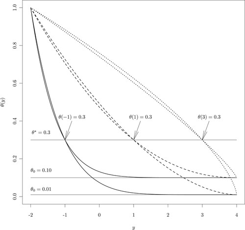
Table 4. Choices for the target toxicity tolerance probability functions by (10(10) $\begin{array}{rl}{\theta }_{\alpha }& ={\theta }_{\alpha }\left(y\right)\\ & =\left\{\begin{array}{ll}1,& \mathrm{i}\mathrm{f}y\le y_0,\\ {\theta }_0+(1-{\theta }_0){\left(\frac{y_1-y}{y_1-y_0}\right)}^{\alpha },& \mathrm{i}\mathrm{f}{y}_0<y<y_1,\\ {\theta }_0,& \mathrm{i}\mathrm{f}y\ge y_1,\end{array}\right.\end{array}$(10) ).

$(y_0,y_1)$	${\theta }_0$	${\theta }^{\ast }$	$y^{\ast }$	α
$(-2,4)$	0.10	0.3	$-1$	8.2496
$(-2,4)$	0.10	0.3	1	2.1699
$(-2,4)$	0.10	0.3	3	0.8394
$(-2,4)$	0.01	0.3	$-1$	6.7344
$(-2,4)$	0.01	0.3	1	1.7714
$(-2,4)$	0.01	0.3	3	0.6853

Notice that, in Figure 4, the trend of $\theta \left(y\right)$ changes with different values of ${\theta }^{\ast }=\theta \left(y^{\ast }\right)$ and ${\theta }_0$. When $y^{\ast }$ increases from $-1$ to 3, $\theta \left(y\right)$ reaches to ${\theta }_0$ in a slower pace. This means that the target tolerance probability curve decreases from 1 to ${\theta }_0$ in a slower rate.

Using the target toxicity tolerance probability curves, simulation results in obtaining the MTD's for the same normal-response model investigated in Section 4.3 are shown in Table 5. In Table 5, the recommended MTD dosage level increases as $y^{\ast }$ increases. When the variance of the toxicity response is larger, the recommended MTD levels spread out more than those with smaller variances.

Table 5. Simulation results of the recommended MTD levels, as well as dosage allocation percentages for different choices of ${\theta }^{\ast }$ and $y^{\ast }$.

		Dose level
${\sigma }^2$	$y^{\ast }$	$d_1$	$d_2$	$d_3$	$d_4$	$d_5$	$d_6$
		${\theta }_0=0.01$
0.25	−1	24.5 (33.35)	75.5 (65.65)	0.0 (1.00)
	1	2.0 (12.80)	83.0 (64.90)	15.0 (21.60)	0.0 (7.00)
	3	0.5 (11.65)	51.0 (41.85)	47.0 (42.75)	1.5 (3.75)
1	−1	49.0 (59.75)	48.0 (37.40)	3.0 (2.75)	0.0 (0.10)
	1	1.0 (15.55)	10.5 (17.55)	73.0 (47.55)	15.5 (18.00)	0.0 (1.35)
	3	0.0 (14.70)	2.0 (11.75)	33.0 (25.00)	50.5 (35.00)	14.5 (12.75)	0.0 (0.80)
2	−1	83.0 (86.20)	15.5 (12.80)	1.5 (1.00)
	1	5.0 (22.90)	18.0 (19.15)	39.0 (29.95)	0.0 (22.70)	4.0 (5.05)	0.0 (0.25)
	3	2.0 (21.65)	6.0 (14.15)	18.5 (18.95)	40.0 (25.40)	30.5 (17.35)	0.25 (2.50)
		${\theta }_0=0.10$
0.25	−1	31.0 (38.05)	69.0 (61.10)	0.0 (0.85)
	1	2.5 (12.10)	86.0 (68.20)	11.5 (19.20)	0.0 (0.50)
	3	1.0 (10.90)	53.0 (43.45)	45.0 (42.65)	1.0 (3.00)
1	−1	47.5 (56.80)	51.0 (40.45)	1.5 (2.65)	0.0 (0.10)
	1	1.0 (12.50)	17.5 (20.95)	67.0 (49.20)	14.5 (16.25)	0.0 (1.10)
	3	0.5 (11.70)	3.5 (11.85)	32.5 (27.00)	55.0 (37.50)	8.5 (11.25)	0.0 (0.70)
2	−1	76.5 (79.35)	23.0 (19.00)	0.5 (1.65)
	1	2.0 (16.70)	17.5 (20.45)	45.5 (33.55)	32.0 (23.75)	3.0 (5.40)	0.0 (0.15)
	3	0.0 (14.15)	1.0 (10.65)	6.0 (13.90)	36.5 (25.15)	51.0 (28.75)	5.5 (7.40)

Finally in this section, we consider a situation that is similar to a dichotomous case, although the toxicity response is still set as normal distribution in Section 4.3. However, the target toxicity probability curve is set as $h(y,y_0,y_1)=\left\{\begin{array}{ll}1,& \mathrm{i}\mathrm{f}-2\le y<1,\\ 0.3,& \mathrm{i}\mathrm{f}1\le y\le 4.\end{array}\right.$In this situation, the level-y MTD can be expressed as $\begin{array}{rl}& {}_y\text{MTD}\left(h\right(y,y_0,y_1)\\ & =\left\{\begin{array}{ll}\frac{y-\sigma {\mathrm{\Phi }}^{-1}\left(0\right)-{\text{β}}_0}{{\text{β}}_1}=\mathrm{\infty },& \mathrm{i}\mathrm{f}-2\le y<1,\\ \frac{y-\sigma {\mathrm{\Phi }}^{-1}\left(0.7\right)-{\text{β}}_0}{{\text{β}}_1}\\ =\frac{y-0.5244\sigma -{\text{β}}_0}{{\text{β}}_1},& \mathrm{i}\mathrm{f}2581\le y\le 4,\end{array}\right.\end{array}$The overall MTD thus can be obtained accordingly. A simulation study for this model is given in Table 6.

Table 6. Simulation results of the recommended MTD levels, as well as dosage allocation percentages for ‘dichotomous’ cases. Two decision criteria are employed: criterion I is to choose next dosage level at a nearest dose, and criterion II is to choose next dosage level at the lower bound.

		Dose level
	${\sigma }^2$	$d_1$	$d_2$	$d_3$	$d_4$	$d_5$	$d_6$
Criterion I	0.25	0.0 (10.30)	0.0 (10.00)	0.0 (10.00)	22.5 (21.85)	77.5 (47.70)	0.0 (0.15)
	1	0.0 (10.50)	0.0 (10.05)	3.5 (12.45)	56.0 (39.40)	40.0 (25.80)	0.5 (1.80)
	2	0.5 (14.50)	3.5 (12.85)	21.0 (21.15)	50.5 (31.90)	24.0 (17.85)	0.5 (1.75)
Criterion II	0.25	0.0 (10.15)	0.0 (10.10)	0.5 (10.45)	91.5 (60.30)	8.0 (8.95)	0.0 (0.05)
	1	0.0 (10.10)	0.0 (10.40)	15.0 (18.85)	48.2 (32.20)	8.0 (10.95)	0.0 (0.50)
	2	1.5 (15.15)	14.0 (18.75)	26.0 (25.15)	52.0 (31.90)	6.5 (8.05)	0.0 (0.70)

In Table 6, two MTD dosage selection criteria are used. Criterion I chooses the next level MTD by the form in (16(16) $x_{j+1}=\underset{x\in \{d_1,\dots ,d_K\}}{\mathrm{a}\mathrm{r}\mathrm{g}\mathrm{m}\mathrm{i}\mathrm{n}}\left\{|x{-}^{\mathbb{Y}}\widehat{\mathrm{M}\mathrm{T}\mathrm{D}}\right({\theta }_{\alpha }\left)|\right\},$(16) ), where a dose level that has nearest distance to ${}^{\mathbb{Y}}\widehat{\mathrm{M}\mathrm{T}\mathrm{D}}\left(\theta \right)$ is chosen, while Criterion II chooses the next level MTD by choosing the largest dose level that is no larger than ${}^{\mathbb{Y}}\widehat{\mathrm{M}\mathrm{T}\mathrm{D}}\left(\theta \right)$. The justification of Criterion II is that we choose next dose level in a more conservative way. In Table 6, we observe that most of the time, level $d_4$ is chosen, unless when $\sigma =0.5$, Criterion I chooses $d_5$. Since we know the true model in this case, we can calculate the toxicity probability at $d_4$ and $d_5$ as $P(Y>1|d_4)=(0.28,0.20,0.05)$, for ${\sigma }^2=(2,1,0.25)$, respectively, and $P(Y>1|d_5)=0.5$ for all ${\sigma }^2$. Hence, it is more aggressive, i.e., with more risk, in using Criterion I for the case of a smaller variance.

5. Conclusions and discussions

In this study, we propose a new framework of determining the maximum tolerated dose for a single toxicity response in clinical trial study. We have a new definition as overall MTD, ${}^{\mathbb{Y}}\mathrm{M}\mathrm{T}\mathrm{D}\left(\theta \right)$, which yields a unified model for the dose finding problem in Phase I clinical trials. The analytic properties of the overall MTD are examined. We prove the Convergence, Robustness and Reduction theorems of the overall MTD. It is shown that the traditional definition of MTD in the case of the dichotomous toxicity responses (see O'Quigley et al., 1990; Yang et al., 2010) as well as the overall MTD, ${}^{\mathit{M}}\mathrm{M}\mathrm{T}\mathrm{D}\left(\mathit{\theta }\right)$, introduced in the polychotomous toxicity responses (Yang & Ye, 2012), are special cases of this more generally defined overall MTD. In other words, this unified model makes it possible to consider the dichotomous, polychotomous and continuous toxicity responses under the same framework.

In order to find the overall MTD, the target toxicity tolerance probability $\theta \left(y\right)$, that corresponds to the level-y severe toxicity $T_y$, for $y\in \mathbb{Y}$, needs to be pre-specified. In the cases of dichotomous and polychotomous toxicity responses, the determination of $\theta \left(y\right)$, $y\in \mathbb{Y}$, is relatively straightforward (see for instance, Yang & Ye, 2012). In the case of continuous toxicity response, one needs to interact with the physicians to obtain an acceptable target toxicity tolerance probability curve $\theta \left(y\right)$. In general, the higher the toxicity tolerance level, the lower the chance that the patient exposes to the toxicity is allowed, i.e., the target toxicity tolerance probability $\theta \left(y\right)$ is decreasing in y, where $y\in \mathbb{Y}$. For all $y\in \mathbb{Y}$, ${\theta }_0\le \theta \left(y\right)\le 1$. A lower bound ${\theta }_0>0$ is necessary for the continuous toxicity response. Otherwise, if $\underset{y\in \mathbb{Y}}{inf}\left\{\theta \right(y\left)\right\}=0$, ${}^{\mathbb{Y}}\mathrm{M}\mathrm{T}\mathrm{D}\left(\theta \right)=-\mathrm{\infty }$ according to (7(7) $\begin{array}{rl}& {}_y\mathrm{M}\mathrm{T}\mathrm{D}\left(h\right(y,y_0,y_1\left)\right)\\ & =\left\{\begin{array}{ll}\mathrm{\infty },y-\sigma F^{-1}[1-& \text{for }y\le y_0,\\ \frac{h(y,y_0,y_1)]-{\text{β}}_0}{{\text{β}}_1},& \text{for }y\in (y_0,y_1),\\ \frac{y-\sigma F^{-1}(1-{\theta }_0)-{\text{β}}_0}{{\text{β}}_1},& \text{for }y\ge y_1.\end{array}\right.\end{array}$(7) ). This will be impractical.

As an example for the continuous case, the normal toxicity response with linear mean in dosage is studied in this research. According to Corollary 2.1 and Proposition 3.3, the normal toxicity system could reduce to the dichotomous probit system described in Yang et al. (2010), as the power α in target toxicity tolerance probability (10(10) $\begin{array}{rl}{\theta }_{\alpha }& ={\theta }_{\alpha }\left(y\right)\\ & =\left\{\begin{array}{ll}1,& \mathrm{i}\mathrm{f}y\le y_0,\\ {\theta }_0+(1-{\theta }_0){\left(\frac{y_1-y}{y_1-y_0}\right)}^{\alpha },& \mathrm{i}\mathrm{f}{y}_0<y<y_1,\\ {\theta }_0,& \mathrm{i}\mathrm{f}y\ge y_1,\end{array}\right.\end{array}$(10) ) goes to infinity. This indicates that the proposed framework is closed under the normal distribution. In addition, we may also use a different target toxicity tolerance probability curve for the normal-response model to reach similar dichotomous response result, such as shown in Section 4.4. Furthermore, we perform several simulation studies and it is shown that the unified model works well for the normal-toxicity responses.

In practice, other continuous toxicity models, such as logistic, beta if the toxicity is represented in percentage or other suitable models, can be utilised under the same framework. Prior elicitation is also an important issue. In this study, we provide full conditional distributions for the parameters for various priors. When more complex models or hard-to-deal-with priors are used, complex full conditional distributions may be encountered, and the difficulties of simulation may arise. However, many simulation methods can be applied to handle those difficulties, such as acceptance-rejection algorithms or Metropolis-Hastings algorithm.

Acknowledgements

Research of Keying Ye and Min Wang were partially supported by grants from the College of Business at the University of Texas at San Antonio.

Disclosure statement

No potential conflict of interest was reported by the author(s).

Additional information

Notes on contributors

Keying Ye

Keying Ye is a professor of Statistics in the Department of Management Science and Statistics at the University of Texas at San Antonio. His research interests include Bayesian analysis, statistical inference and decision theory, and statistical applications.

Xiaobin Yang

Xiaobin Yang is a senior statistician in the HouseCanary Inc., San Antonio, Texas. His research interests include statistical analysis and applications.

Ying Ji

Ying Ji is a statistical consultant and her research interests include statistical analysis and applications.

Min Wang

Min Wang is an associate professor of Statistics in the Department of Management Science and Statistics at the University of Texas at San Antonio. His research interests include Bayesian statistics, high dimensional inference and statistical applications and machine learning.

Appendix

Proof

Proof of Lemma 2.1.

Since, for all $y\in \mathbb{Y}$, $\underset{y\in \mathbb{Y}}{inf}\left\{g\right(y)-g_0(y\left)\right\}\le g\left(y\right)-g_0\left(y\right)\le \underset{y\in \mathbb{Y}}{sup}\left\{g\right(y)-g_0(y\left)\right\}$, we have $\underset{y\in \mathbb{Y}}{inf}\left\{g\right(y)-g_0(y\left)\right\}+g_0\left(y\right)\le g\left(y\right)-g_0\left(y\right)+g_0\left(y\right)\le \underset{y\in \mathbb{Y}}{sup}\left\{g\right(y)-g_0(y\left)\right\}+g_0\left(y\right)$. Therefore, $\begin{array}{rl}& \underset{y\in \mathbb{Y}}{inf}\left\{g\right(y)-g_0(y\left)\right\}+\underset{y\in \mathbb{Y}}{inf}\left\{g_0\right(y\left)\right\}\le \underset{y\in \mathbb{Y}}{inf}\left\{g\right(y\left)\right\}\\ & \le \underset{y\in \mathbb{Y}}{sup}\left\{g\right(y)-g_0(y\left)\right\}+\underset{y\in \mathbb{Y}}{inf}\left\{g_0\right(y\left)\right\}.\end{array}$Consequently, the fact is proved by subtracting $\underset{y\in \mathbb{Y}}{inf}\left\{g_0\right(y\left)\right\}$ on each side of both inequalities because $\underset{y\in \mathbb{Y}}{inf}\left\{g_0\right(y\left)\right\}<\mathrm{\infty }$ since $|g_0\left(y\right)|<\mathrm{\infty }$.

Proof

Proof of Theorem 2.1.

For all $y\in \mathbb{Y}$, denote $h_y\left(x\right)\triangleq P(Y<y|x)$. According to the regularity condition, $h_y\left(x\right)$ is continuous and strictly decreasing in x. Hence $h_y^{-1}\left(x\right)$ is also continuous and strictly decreasing in x, where $h_y^{-1}$ is the inverse function of $h_y$. Therefore, according to (2.2), the level-y MTD for toxicity system $(\mathbb{Y},\mathit{F},{\theta }_n)$ is $\begin{array}{rl}{}_y\mathrm{M}\mathrm{T}\mathrm{D}\left({\theta }_n\right(y\left)\right)& =sup\left\{x|P\right(Y<y|x)\ge 1-{\theta }_n(y\left)\right\}\\ & =sup\left\{x|h_y\right(x)\ge 1-{\theta }_n(y\left)\right\}\\ & =sup\{x|x\ge h_y^{-1}(1-{\theta }_n\left(y\right)\left)\right\}\\ & =h_y^{-1}(1-{\theta }_n(y\left)\right),\end{array}$where $n=0,1,2,\dots$. Since $h_y^{-1}$ is continuous, one has, for any $ϵ>0$, there exists a $\delta >0$, such that if $|{\theta }_n\left(y\right)-{\theta }_0\left(y\right)|<\delta$, then $\begin{array}{rl}& |{}_y\mathrm{M}\mathrm{T}\mathrm{D}\left({\theta }_n\right(y\left)\right)-{}_y\mathrm{M}\mathrm{T}\mathrm{D}\left({\theta }_0\right(y\left)\right)|\\ & =|h_y^{-1}\left({\theta }_n\right(y\left)\right)-h_y^{-1}\left({\theta }_0\right(y\left)\right)|<ϵ.\end{array}$Since ${\theta }_n$ uniformly converges to ${\theta }_0$, for the $\delta >0$, there exists an N>0, such that for all n>N and $y\in \mathbb{Y}$, $|{\theta }_n\left(y\right)-{\theta }_0\left(y\right)|<\delta$.

Consequently, for any $ϵ>0$, there exists a N>0, such that for all n>N and $y\in \mathbb{Y}$, $-ϵ<{}_y\mathrm{M}\mathrm{T}\mathrm{D}\left({\theta }_n\right(y\left)\right)-{}_y\mathrm{M}\mathrm{T}\mathrm{D}\left({\theta }_0\right(y\left)\right)<ϵ.$Furthermore, according to Lemma 2.1, we have $-ϵ<\underset{y\in \mathbb{Y}}{inf}\left\{{}_y\mathrm{M}\mathrm{T}\mathrm{D}\right({\theta }_n\left(y\right)\left)\right\}-\underset{y\in \mathbb{Y}}{inf}\left\{{}_y\mathrm{M}\mathrm{T}\mathrm{D}\right({\theta }_0\left(y\right)\left)\right\}<ϵ,$or, $-ϵ<{}^{\mathbb{Y}}\mathrm{M}\mathrm{T}\mathrm{D}\left({\theta }_n\right)-{}^{\mathbb{Y}}\mathrm{M}\mathrm{T}\mathrm{D}\left({\theta }_0\right)<ϵ,$which implies that $\underset{n\to \mathrm{\infty }}{lim}{}^{\mathbb{Y}}\mathrm{M}\mathrm{T}\mathrm{D}\left({\theta }_n\right)={}^{\mathbb{Y}}\mathrm{M}\mathrm{T}\mathrm{D}\left({\theta }_0\right)$.

Proof

Proof of Theorem 2.3.

Let ${}^{\mathbb{Y}}\mathrm{M}\mathrm{T}\mathrm{D}\left(\theta \right)$ and ${}^{{\mathbb{Y}}^{\mathbb{\ast }}}{\mathrm{M}\mathrm{T}\mathrm{D}}^{\ast }\left({\theta }^{\ast }\right)$ denote the overall MTD of toxicity systems $(\mathbb{Y},\mathit{F},\theta )$ and $({\mathbb{Y}}^{\ast },{\mathit{F}}^{\ast },{\theta }^{\ast })$, respectively. Since $\theta \left(y\right)\ge \theta \left(y_1\right)$ for all $y_1\le y<y_2$, using Propositions 2.1 and 2.2, we have, $\begin{array}{rl}& {}_{y_1}\mathrm{M}\mathrm{T}\mathrm{D}\left(\theta \right(y_1\left)\right)\le {}_y\mathrm{M}\mathrm{T}\mathrm{D}\left(\theta \right(y_1\left)\right){\le }_y\mathrm{M}\mathrm{T}\mathrm{D}\left(\theta \right(y\left)\right),\\ & \mathrm{f}\mathrm{o}\mathrm{r}\mathrm{a}\mathrm{l}\mathrm{l}{y}_1\le y<y_2,\end{array}$where ${}_y\mathrm{M}\mathrm{T}\mathrm{D}\left(\theta \right(y\left)\right)$ is the level-y MTD associated with system $(\mathbb{Y},\mathit{F},\theta )$. Hence, (A1) $\begin{array}{rl}{}^{\mathbb{Y}}\mathrm{M}\mathrm{T}\mathrm{D}\left(\theta \right)& =inf\left\{{}_y\mathrm{M}\mathrm{T}\mathrm{D}\right(\theta \left(y\right))|y\in \mathbb{Y}\}\\ & =inf\left\{{}_y\mathrm{M}\mathrm{T}\mathrm{D}\right(\theta \left(y\right))|y\in {\mathbb{Y}}^{\ast }\}.\end{array}$(A1) Using (4(4) $F^{\ast }\left(y|x\right)=\left\{\begin{array}{ll}F\left(y|x\right),& \text{if }y<y_1\text{ or }y\ge y_2,\\ F\left(y_2|x\right),& \text{if }{y}_1\le y<y_2,\end{array}\right.$(4) ) and ${\theta }^{\ast }=\theta \left(y\right),y\in {\mathbb{Y}}^{\ast }$, we have $\begin{array}{rl}& \{x\in \mathbb{X}|F^{\ast }(y|x)\ge 1-{\theta }^{\ast }(y\left)\right\}\\ & =\{x\in \mathbb{X}|F(y|x)\ge 1-\theta (y\left)\right\},\mathrm{f}\mathrm{o}\mathrm{r}\mathrm{a}\mathrm{l}\mathrm{l}y\in {\mathbb{Y}}^{\ast }.\end{array}$Hence, according to (2.2), ${}_y{\mathrm{M}\mathrm{T}\mathrm{D}}^{\ast }\left({\theta }^{\ast }\right(y\left)\right)={}_y\mathrm{M}\mathrm{T}\mathrm{D}\left(\theta \right(y\left)\right)$, for all $y\in {\mathbb{Y}}^{\ast }$, where ${}_y{\mathrm{M}\mathrm{T}\mathrm{D}}^{\ast }\left({\theta }^{\ast }\right(y\left)\right)$ is the level-y MTD associated with system $({\mathbb{Y}}^{\ast },{\mathit{F}}^{\ast },{\theta }^{\ast })$. Finally, using (A1(A1) $\begin{array}{rl}{}^{\mathbb{Y}}\mathrm{M}\mathrm{T}\mathrm{D}\left(\theta \right)& =inf\left\{{}_y\mathrm{M}\mathrm{T}\mathrm{D}\right(\theta \left(y\right))|y\in \mathbb{Y}\}\\ & =inf\left\{{}_y\mathrm{M}\mathrm{T}\mathrm{D}\right(\theta \left(y\right))|y\in {\mathbb{Y}}^{\ast }\}.\end{array}$(A1) ), $\begin{array}{rl}{}^{\mathbb{Y}}\mathrm{M}\mathrm{T}\mathrm{D}\left(\theta \right)& =inf\left\{{}_y\mathrm{M}\mathrm{T}\mathrm{D}\right(\theta \left(y\right))|y\in {\mathbb{Y}}^{\ast }\}\\ & =inf\left\{{}_y{\mathrm{M}\mathrm{T}\mathrm{D}}^{\ast }\right({\theta }^{\ast }\left(y\right))|y\in {\mathbb{Y}}^{\ast }\}\\ & ={}^{{\mathbb{Y}}^{\mathbb{\ast }}}{\mathrm{M}\mathrm{T}\mathrm{D}}^{\ast }\left({\theta }^{\ast }\right)\end{array}$which implies that system $(\mathbb{Y},\mathit{F},\theta )$ is equivalent to system $({\mathbb{Y}}^{\ast },{\mathit{F}}^{\ast },{\theta }^{\ast })$ in the sense of finding the overall MTD.

Proof

Proof of Proposition 3.3.

Since $\left[\right(y_1-y\left)/\right(y_1-y_0){]}^{\alpha }$ is decreasing in α, for any $y\in (y_0,y_1)$, it is easy to show that the overall MTD in (11(11) $\begin{array}{r}{}^{\mathbb{Y}}\mathrm{M}\mathrm{T}\mathrm{D}\left({\theta }_{\alpha }\right)=\underset{y\in (y_0,y_1)}{inf}\left\{\begin{array}{c}y-\sigma {\mathrm{\Phi }}^{-1}\left\{\right(1-{\theta }_0)\\ \times [1-(\frac{y_1-y}{y_1-y_0}{)}^{\alpha }\left]\right\}-{\text{β}}_0\end{array}\right\}{\text{β}}_1^{-1}.\end{array}$(11) ) is decreasing in α.

Since ${\mathrm{\Phi }}^{-1}\left[\right(1-{\theta }_0\left)\right(1-\left[\frac{y_1-y}{y_1-y_0}{]}^{\alpha }\right)]$ is continuously increasing in α, we have $\underset{\alpha \to \mathrm{\infty }}{lim}{\mathrm{\Phi }}^{-1}\left[(1-{\theta }_0)\left(1-{\left[\frac{y_1-y}{y_1-y_0}\right]}^{\alpha }\right)\right]={\mathrm{\Phi }}^{-1}(1-{\theta }_0),$ for any $y\in (y_0,y_1)$, which implies that for any $ϵ>0$, there exists a real number A, such that for any $\alpha >A$, $-\frac{{\text{β}}_1ϵ}{\sigma }<{\mathrm{\Phi }}^{-1}\left[(1-{\theta }_0)\left(1-{\left[\frac{y_1-y}{y_1-y_0}\right]}^{\alpha }\right)\right]-{\mathrm{\Phi }}^{-1}\left({\theta }_1\right)<0,$for any $y\in (y_0,y_1)$. Hence, for any $ϵ>0$, there exists a real number A, such that for any $\alpha >A$, $\begin{array}{rl}0& <\underset{y\in (y_0,y_1)}{inf}\left\{\frac{y-\sigma {\mathrm{\Phi }}^{-1}\left[(1-{\theta }_0)\left(1-{\left[{\displaystyle \frac{y_1-y}{y_1-y_0}}\right]}^{\alpha }\right)\right]-{\text{β}}_0}{{\text{β}}_1}\right\}\\ & -\frac{y_0-\sigma {\mathrm{\Phi }}^{-1}(1-{\theta }_0)-{\text{β}}_0}{{\text{β}}_1}\\ & =\underset{y\in (y_0,y_1)}{inf}\left\{\begin{array}{l}(y-y_0)-\sigma \left({\mathrm{\Phi }}^{-1}\left[(1-{\theta }_0)\phantom{\left(1-{\left[\frac{y_1-y}{y_1-y_0}\right]}^{\alpha }\right)}\right.\right.\\ \left.\left(1-{\left[\frac{y_1-y}{y_1-y_0}\right]}^{\alpha }\right)\right]-{\mathrm{\Phi }}^{-1}(1-{\theta }_0))\end{array}\right\}{\text{β}}_1^{-1}\\ & <\underset{y\in (y_0,y_1)}{inf}\left\{\frac{y-y_0}{{\text{β}}_1}\right\}+ϵ=ϵ,\end{array}$

which implies (12(12) $\begin{array}{rl}\underset{\alpha \to \mathrm{\infty }}{lim}{}^{\mathbb{Y}}\mathrm{M}\mathrm{T}\mathrm{D}\left({\theta }_{\alpha }\right)& =\frac{y_0-\sigma {\mathrm{\Phi }}^{-1}(1-{\theta }_0)-{\text{β}}_0}{{\text{β}}_1}\\ & =\frac{y_0+\sigma {\mathrm{\Phi }}^{-1}\left({\theta }_0\right)-{\text{β}}_0}{{\text{β}}_1},\end{array}$(12) ).

References

- Bekele, B. N., & Thall, P. F. (2004). Dose-finding based on multiple toxicities in a soft tissue Sarcoma trial. Journal of the American Statistical Association, 99(465), 26–35. https://doi.org/https://doi.org/10.1198/016214504000000043
- Braun, T. M. (2002). The bivariate continual reassessment method: extending the CRM to phase I trials of two competing outcomes. Controlled Clinical Trials, 23(3), 240–256. https://doi.org/https://doi.org/10.1016/S0197-2456(01)00205-7
- Cheng, B., & Lee, S. M. (2015). On the consistency of the continual reassessment method with multiple toxicity constraints. Journal of Statistical Planning and Inference, 164, 1–9. https://doi.org/https://doi.org/10.1016/j.jspi.2015.03.001
- Chevret, S. (1993). The continual reassessment method in cancer phase i clinical trials: A simulation study. Statistics in Medicine, 12(12), 1093–1108. https://doi.org/https://doi.org/10.1002/sim.v12:12
- Clertant, M., & O'Quigley, J. (2017). Semiparametric dose finding methods. Journal of the Royal Statistical Society: Series B (Statistical Methodology), 79(5), 1487–1508. https://doi.org/https://doi.org/10.1111/rssb.2017.79.issue-5
- Clertant, M., & O'Quigley, J. (2019). Semiparametric dose finding methods. Journal of the Royal Statistical Society: Series C (Applied Statistics), 68(2), 271–288. https://doi.org/https://doi.org/10.1111/rssc.12308
- Faries, D. (1994). Practical modifications of the continual reassessment method for phase I cancer clinical trials. Journal of Biopharmaceutical Statistics, 4(2), 147–164. https://doi.org/https://doi.org/10.1080/10543409408835079
- Goodman, S. N., Zahurak, M. L., & Piantadosi, S. (1995). Some practical improvements in the continual reassessment method for phase I studies. Statistics in Medicine, 14(11), 1149–1161. https://doi.org/https://doi.org/10.1002/(ISSN)1097-0258
- Gooley, T. A., Martin, P. J., Fisher, L. D., & Pettinger, M. (1994). Simulation as a design tool for phase I/II clinical trials: An example from bone marrow transplantation. Controlled Clinical Trials, 15(6), 450–462. https://doi.org/https://doi.org/10.1016/0197-2456(94)90003-5
- Heyd, J. M., & Carlin, B. P. (1999). Adaptive design improvements in the continual reassessment method for phase I studies. Statistics in Medicine, 18, 1307–1321. https://doi.org/https://doi.org/10.1002/(ISSN)1097-0258
- Iasonos, A., Wilton, A. S., Riedel, E. R., Seshan, V. E., & Spriggs, D. R. (2008). A comprehensive comparison of the continual reassessment method to the standard 3 + 3 dose escalation scheme in phase I dose-finding studies. Clinical Trials, 5(5), 465–477. https://doi.org/https://doi.org/10.1177/1740774508096474
- Ishizuka, N., & Ohashi, Y. (2001). The continual reassessment method and its applications: a Bayesian methodology for phase I cancer clinical trials. Statistics in Medicine, 20(17–18), 2661–2681. https://doi.org/https://doi.org/10.1002/(ISSN)1097-0258
- Ji, L., Lewinger, J. P., Krailo, M., Groshen, S., Conti, D. V., Asgharzadeh, S., & Sposto, R. (2019). Improvements to the escalation with overdose control design and a comparison with the restricted continual reassessment method. Pharmaceutical Statistics, 18(6), 659–670. https://doi.org/https://doi.org/10.1002/pst.v18.6
- Korn, E. L., Midthune, D., Chen, T. T., Rubinstein, L. V., Christian, M. C., & Simon, R. M. (1994). A comparison of two phase I trial designs. Statistics in Medicine, 13(18), 1799–1806. https://doi.org/https://doi.org/10.1002/(ISSN)1097-0258
- Liu, S., Pan, H., Xia, J., Huang, Q., & Yuan, Y. (2015). Bridging continual reassessment method for phase I clinical trials in different ethnic populations. Statistics in Medicine, 34(10), 1681–1694. https://doi.org/https://doi.org/10.1002/sim.v34.10
- Morita, S. (2011). Application of the continual reassessment method to a phase I dose-finding trial in Japanese patients: East meets West. Statistics in Medicine, 30(17), 2090–2097. https://doi.org/https://doi.org/10.1002/sim.3999
- National Cancer Institute (1999). Common toxicity criteria manual, version 2.0 (pp. 1–22). National Cancer Institute.
- North, B., Kocher, H. M., & Sasieni, P. (2019). A new pragmatic design for dose escalation in phase 1 clinical trials using an adaptive continual reassessment method. BMC Cancers, 19(1), Article ID 632. https://doi.org/https://doi.org/10.1186/s12885-019-5801-3https://rdcu.be/b0l2z
- Onar, A., Kocak, M., & Boyett, J. M. (2009). Continual reassessment method vs. traditional empirically based design: modifications motivated by phase I trials in pediatric oncology by the pediatric brain tumor consortium. Journal of Biopharmaceutical Statistics, 19(3), 437–455. https://doi.org/https://doi.org/10.1080/10543400902800486
- Onimaru, R., Shirato, H., Shibata, T., Hiraoka, M., Ishikura, S., Karasawa, K., Matsuo, Y., Kokubo, M., Shioyama, Y., Matsushita, H., Ito, Y., & Onishi, H. (2015). Phase I study of stereotactic body radiation therapy for peripheral T2N0M0 non-small cell lung cancer with PTV < 100 cc using a continual reassessment method (JCOG0702). Radiotherapy and Oncology, 116(2), 276–280. https://doi.org/https://doi.org/10.1016/j.radonc.2015.07.008
- O'Quigley, J. (1992). Estimating the probability of toxicity at the recommended dose following a phase I clinical trial in cancer. Biometrics, 48(3), 853–862. https://doi.org/https://doi.org/10.2307/2532350
- O'Quigley, J. (2002). Continual reassessment designs with early termination. Biostatistics, 3(1), 87–99. https://doi.org/https://doi.org/10.1093/biostatistics/3.1.87
- O'Quigley, J., & Chevret, S. (1991). Methods for dose finding studies in cancer clinical trials: A review and results of a Monte Carlo study. Statistics in Medicine, 10(11), 1647–1664. https://doi.org/https://doi.org/10.1002/(ISSN)1097-0258
- O'Quigley, J., Pepe, M., & Fisher, L. (1990). Continual reassessment method: A practical design for phase I clinical trials in cancer. Biometrics, 46(1), 33–48. https://doi.org/https://doi.org/10.2307/2531628
- O'Quigley, J., & Reiner, E. (1998). A stopping rule for the continual reassessment method. Biometrika, 85(3), 741–748. https://doi.org/https://doi.org/10.1093/biomet/85.3.741
- Piantadosi, S., & Liu, G. (1996). Improved designs for dose escalation studies using pharmacokinetic measurements. Statistics in Medicine, 15, 1605–1618. https://doi.org/https://doi.org/10.1002/(ISSN)1097-0258
- Salter, A., Morgan, C., & Aban, I. B. (2015). Implementation of a two-group likelihood time-to-event continual reassessment method using SAS. Computer Methods and Programs in Biomedicine, 121(3), 189–196. https://doi.org/https://doi.org/10.1016/j.cmpb.2015.06.001
- Storer, B. E. (2001). An evaluation of phase I clinical trial designs in the continuous dose-response setting. Statistics in Medicine, 20(16), 2399–2408. https://doi.org/https://doi.org/10.1002/(ISSN)1097-0258
- Thall, P. F., & Lee, S. J. (2003). Practical model-based dose-finding in phase I clinical trials: Methods based on toxicity. International Journal of Gynecological Cancer, 13(3), 251–261. https://doi.org/https://doi.org/10.1046/j.1525-1438.2003.13202.x
- Wang, C., Chen, T. T., & Tyan, I. (2000). Designs foe phase I cancer clinical trials with differentiation of graded toxicity. Communications in Statistics - Theory and Methods, 29(5–6), 975–987. https://doi.org/https://doi.org/10.1080/03610920008832527
- Yang, X., & Ye, K. (2012). A phase I dose-finding study based on polychotomous toxicity responses. Statistics and Its Inference, 5, 451–461.https://doi.org/https://doi.org/10.4310/SII.2012.v5.n4.a8
- Yang, X., Ye, K., & Wang, Y. (2010). A study of the probit model with latent variables in phase I clinical trials. Working Paper Series 0030, College of Business, University of Texas at San Antonio.
- Yuan, Z., Chappell, R., & Bailey, H. (2007). The continual reassessment method for multiple toxicity grades: A Bayesian quasi-likelihood approach. Biometrics, 63(1), 173–179. https://doi.org/https://doi.org/10.1111/biom.2007.63.issue-1
- Zhong, W., Koopmeiners, J. S., & Carlin, B. P. (2012). A trivariate continual reassessment method for phase I/II trials of toxicity, efficacy, and surrogate efficacy. Statistics in Medicine, 31(29), 3885–3895. https://doi.org/https://doi.org/10.1002/sim.5477
- Zohar, S., & Chevret, S. (2003). Phase I (or phase II) dose-ranging clinical trials: proposal of a two-stage Bayesian design. Journal of Biopharmaceutical Statistics, 13(1), 87–101. https://doi.org/https://doi.org/10.1081/BIP-120017728
- Zohar, S., Resche-Rigon, M., & Chevret, S. (2011). Using the continual reassessment method to estimate the minimum effective dose in phase II dose-finding studies: a case study. Clinical Trials, 10(3), 414–421. https://doi.org/https://doi.org/10.1177/1740774511411593