An integrated epidemic modelling framework for the real-time forecast of COVID-19 outbreaks in current epicentres

Abstract

Various studies have provided a wide variety of mathematical and statistical models for early epidemic prediction of the COVID-19 outbreaks in Mainland China and other epicentres worldwide. In this paper, we present an integrated modelling framework, which incorporates typical exponential growth models, dynamic systems of compartmental models and statistical approaches, to depict the trends of COVID-19 spreading in 33 most heavily suffering countries. The dynamic system of SIR-X plays the main role for estimation and prediction of the epidemic trajectories showing the effectiveness of containment measures, while the other modelling approaches help determine the infectious period and the basic reproduction number. The modelling framework has reproduced the subexponential scaling law in the growth of confirmed cases and adequate fitting of empirical time-series data has facilitated the efficient forecast of the peak in the case counts of asymptomatic or unidentified infected individuals, the plateau that indicates the saturation at the end of the epidemic growth, as well as the number of daily positive cases for an extended period.

Keywords:

• COVID-19
• statistical model
• SIR-X model
• basic reproduction number
• infectious period

1. Introduction

Starting from Wuhan in early December 2019, a novel severe acute respiratory syndrome coronavirus, named as COVID-19, prevailed unexpectedly with a detrimental effect on public health. Though mainland China as the first epicentre of COVID-19, had the coronavirus successfully controlled within two months, its initial success has not prevented the beginning of a global pandemic due to the ignorance of the new virus and contempt of its threat. With the first COVID-19 case outside of China reported on January 13 in Thailand, in a short period of time, the unruly contagion boosted promptly in a wide array of countries all over the world, resulting in the continuous shift of the epicentre. In March, the COVID-19 hit massively on Italy, while jumping the fences into other countries of the European Union. At the same period of time, it cropped up in Iran, and the cumulative number surged to the peak by the end of March, radiating the Middle East and part of Central Asia. Followed after Europe, the USA took over and became the most infected country in the world with the highest total cases ever since. In April, Russia began to suffer seriously in consequence of the failure of lockdown. From May, more positive cases have been emerging in a wide range of countries of Latin America, with the new epicentres mainly consisting of Brazil, Mexico, Chile and Peru. India, along with Pakistan and Bangladesh in South Asia, has been triggered to an epidemic explosion around late May. After June, Africa became the latest epicentre with abounding underestimated positive cases in most of the African countries due to their limited conditions of detection. By mid-July, over 13 million people have been infected, with more than 500 thousands deaths worldwide. Currently, the highest incidences appear in the USA and the epidemic situation keeps deteriorating at a rapid growth rate in a great number of developing countries. The COVID-19 has been continuing sweeping the globe at a tremendous speed, bringing about the massive threat to the public health, economy and numerous aspects of society. Currently, epicentres in Latin America, Africa, part of Asia and Europe continue undergoing the first wave of the outbreaks. The collapse of a nationwide health system, high mortality rate and increasing economic recession have brought forth heavy losses in the vast majority of countries across the globe. As a consequence, the World Health Organisation (WHO) officially announced the outbreak of COVID-19 as a Public Health Emergency of International Concern (PHEIC) on 11 March 2020.

Under such circumstance, academic effort to comprehend the mechanism of the transmissibility is an urgent need to alleviate the negative effects of COVID-19, which will help adequate decision-making related to the public health system and other social and economic aspects. However, limited understanding of the epidemic source and spread remain the crucial problem to be solved. There has emerged a huge literature on modelling studies for COVID-19, starting from simple data-driven approaches concluded by Huang et al. (2020), mostly focusing on the dynamic ODE-based compartmental models, up to the popular machine learning and deep learning methods (see Mohamadou et al., 2020). These modelling tools have been widely employed to study global pandemic from various perspectives, including transmissibility, epidemic prediction, import risk assessment, management strategies and image-based automatic detection.

Apart from the traditional data-driven modelling for epidemiological parameters like $R_0$ and effective reproduction number (see Li et al., 2020; Zhao et al., 2020), enormous number of works mainly focused on the construction of compartmental models aiming to interpret the trends of COVID-19, including the most frequently used Susceptible-Infected-Recovered (SIR) and the Susceptible-Exposed-Infected-Removed (SEIR) models. The SIR model is the basis for epidemiological dynamic systems, which could be easily applied for basic prediction of the trends of COVID-19, see Song et al. (2020), González (2020). Sun et al. (2020) and Chen et al. (2020) proposed a modified SIR model with varying coefficients, vSIR for short, to characterise the time-varying dynamic regimes due to the significant intervention measures implemented by governments of different countries. Via the locally weighted regression given by Cleveland and Devlin (1988) that produces estimates for parameters with desired smoothness, the vSIR model makes the transmission rate α and the effective reproduction number $R_t$ varying with time and possesses the capability for capturing the changing dynamics with guaranteed statistical consistency.

Compared with the SIR, the SEIR model owns an additional compartment ‘E’ (Exposed), which contributes to the flexibility of the infectious period. Among recent studies, Zhao et al. (2020) modelled the epidemic trends of COVID-19 at the early stage and estimated the transmission rate of COVID-19 via $R_0$ based on the data of Wuhan, China from 10 January to 24 January 2020. Tang et al. (2020) proposed a deterministic SEIR compartmental model for COVID-19 spreading. Wu et al. (2020) used a typical SEIR compartmental model to infer the number of infected cases in Wuhan from the data on the number of cases that internationally exported from Wuhan. Later on, various modifications of SEIR were put forward with interesting prediction results. In the study given by Yang et al. (2020), the epidemics trend of COVID-19 in China was predicted under public health interventions. Peng et al. (2020) proposed a generalised SEIR model to analyse the spread of COVID-19 in China. The model can describe the trends of isolated individuals, recovered individuals and dead individuals.

A variety of extensions of compartmental models were derived from traditional SIR and SEIR models to measure the influence of asymptomatic individuals and the effects of intervention (see X. Wang et al., 2020). He et al. (2020) combined the SEIR models with particle swarm optimisation algorithm for parameter optimisation. Liu et al. (2020) proposed a SAIR (Susceptible-Asymptomatic-Infected-Removed) model in the context of social networks where nodes represent individuals and links stand for the contacts between individuals. Rajagopal et al. (2020) developed a SEIRD model with fractional-order derivatives based on the data in Italy and showed that the model has less error than the classical ones. Maier and Brockmann (2020) presented a parsimonious SIR-X model to absorb quarantine measures, containment policies and unidentified infectious individuals (containing asymptomatic patients). In addition to the standard parameters of SIR models, the SIR-X model extends the model with a new compartment ‘X’ to show effective quarantine measures acting on both symptomatic individuals and susceptible individuals. Another series of extension is based on SEIR model to reflect the effectiveness of actual measures like intervention implemented by the government. For instance, Xu et al. (2020) created a complex SEIQRP model with six compartments (Susceptible-Exposed-Infectious-Quarantined-Recovered-Insusceptible) in order to accurately predict the cumulative number of cases. T. Wang et al. (2020) proposed a novel SCEIRD model with susceptible subjects (S), close contacts (C), latent (E, infected and infectious but asymptomatic), infected (I), recovered (R), and dead (D) as its compartments and two new parameters to depict the social transmissibility and the pathologic transmissibility.

The structure of this article is organised as follows. Section 2 briefly describes the modelling framework. Section 3 elaborates the detailed methodologies for our modelling framework. Section 4 describes the model fitting and prediction results. Conclusions and discussions are given in Section 5.

2. Modelling framework

Although a wealth of recent modelling studies has demonstrated well-fitted results obtained from miscellaneous compartmental models, they are particularly dependent on epidemiological parameter estimation and the quality of real data collected in different countries. In this study, in order to overcome the shortage, we propose an integrated modelling framework which consists of three parts: estimation of epidemiological parameters, estimation of infectious period and compartmental models for the dynamic system. The compartmental models focus on the estimation and prediction of the epidemic trajectories and effectiveness of containment measures, while the other two parts play supplementary roles that specifically assess the infectious period and the basic reproduction number of each studied country, which directly determines the two main parameters (the transmission rate α and the recovery rate β) in the dynamic system.

In the first modelling part, we manage to estimate epidemiological parameters for different studied countries. The basic reproduction number $R_0$, the final size of infected and timing of the turning point constitute the crucial epidemiological parameters during an outbreak. These parameters, summarising the temporal pattern of the pandemic, quantify the extent of contagiousness, epidemic severity and the inflection time point, respectively. The estimation of the key epidemiological parameters contributes to the forecast of the trend of transmissibility, which plays a vital role in the planning of containment policies. Inspired by the previous work of Zhao et al. (2019), we adopt classical non-linear phenomenological models, including growth models like Gompertz model (see Gompertz, 1825), logistic model (see Verhulst, 1838) and Richards model (see Richards, 1959), to study the parameters of epidemic features.

In the second modelling part, we introduce another decisive factor, the infectious period $T_I$, that seriously affects the transmissibility. $T_I$ stands for the duration of which pathogens could be transmitted from an infected individual to a susceptible host. It is considered as a critical feature that partly reflexes the extent of intervention, including the efficiency of quarantining the infected population. Here, we employ the statistical framework recently proposed by Lin et al. (2020). This approach is technically based on a time-varying Poisson increment of daily cases, which was proved to be consistent in determining the infectious period of various countries despite spatial heterogeneity.

In the last modelling part, we concentrate on evaluating the transmissibility of the pandemic and checking if the current implemented containment measures are effective in decreasing the spread of the pandemic. Compartmental models, like the SIR models and their derivatives, are among the most commonly applied methodologies in the study of epidemic dynamics. However, the well-fitted results appear to be substantially dependent on the precise estimation of two crucial parameters, basic reproduction number $R_0$ and the infectious period $T_I$, which could be solved by the first two parts of our modelling framework.

We collected the exact number of COVID-19 confirmed positive cases in 33 highly infected countries using the data from 15 February 2020 to 10 July 2020 (with the date of the earliest case reported in a certain country) from the official websites of the World Health Organisation (https://covid19.who.int). Time-dependent incidence data were retrieved, covering a list of current epicentres in five continents: South America, North America, Asia, Africa and Europe. Countries with massive infected population, such as Brazil, India, Mexico, Russia, South Africa, were selected for our study following the basis that they kept the trends of developing within the first wave up to the end of this study. Note that the USA was excluded from our study not only because it has been preponderating over any other countries and demonstrating a unique and steadily-paced growth, but headed for an unknown second crest which is a completely different pattern in contrast to other countries as well.

3. Methods

We now describe the three parts in the integrated modelling framework, which play different roles but closely related to each other.

3.1. Estimation of epidemiological parameters

$R_0$ is the expected number of infections by an infected individual over his/her infectious period at the start of the epidemic, which is closely connected to the time-varying effective reproduction number $R_t$. Both $R_0$ and $R_t$ are key measures of an epidemic. For fixed coefficient models, if $R_0<1$, the epidemic will eventually subside with speed depending on the value of $R_0$; otherwise, an inevitable explosion will occur until the growth ceased by the powerful containment or the rise of mortality.

Mathematical modelling is broadly applied to study the primary features of the pandemic by estimating the epidemiological parameters. Here, we apply a typical epidemiological framework of Zhao et al. (2019) for the estimation of $R_0$. Following previous studies of Wallinga and Lipsitch (2007), the basic reproduction number $R_0$ is given by the Euler–Lotka equation (1) $R_0=\frac{1}{M(-r)}=\frac{1}{{\displaystyle {\int }_0^{\mathrm{\infty }}{\mathrm{e}}^{-r\nu }g\left(\nu \right)\mathrm{d}\nu }},$(1) where r is the intrinsic growth rate from common growth models, and ν is the serial interval (SI) with probability density function $g(\cdot )$. Thus, the function $M(\cdot )$ is the Laplace transformation of $g(\cdot )$, also known as the moment generating function (MGF). The serial interval refers to the average time between clinical onsets in an infector and the corresponding infectees. For our study, SI was estimated using the result of Li et al. (2020) based on the collected information on demographic features, exposure history, and illness onsets of the first 425 confirmed cases which had been reported in Wuhan by 22 January 2020, while its probability density was approximated by a Gamma distribution with a mean of 7.5 days and standard deviation (SD) of 3.4 days, see Li et al. (2020).

Therefore, the intrinsic growth rate r remains to be solved by data-driven process. Three typical growth models are utilised in our attempt to fit the real number of cumulative cases $C\left(t\right)$ (2) $\begin{array}{rl}& \mathrm{L}\mathrm{o}\mathrm{g}\mathrm{i}\mathrm{s}\mathrm{t}\mathrm{i}\mathrm{c}:C\left(t\right)=\frac{K}{1+{\mathrm{e}}^{-r(t-\omega )}},\end{array}$(2) (3) $\begin{array}{rl}& \mathrm{G}\mathrm{o}\mathrm{m}\mathrm{p}\mathrm{e}\mathrm{r}\mathrm{t}\mathrm{z}:C\left(t\right)=K{\mathrm{e}}^{-{\mathrm{e}}^{-r(t-\omega )}},\end{array}$(3) and (4) $\mathrm{R}\mathrm{i}\mathrm{c}\mathrm{h}\mathrm{a}\mathrm{r}\mathrm{d}\mathrm{s}:C\left(t\right)=\frac{K}{[1+\theta {\mathrm{e}}^{-\theta r(t-\omega )}{]}^{\left(1/\theta \right)}}.$(4) The standard nonlinear least square approach is adopted for model fitting to estimate the parameters of K (maximum cumulative case number), ω (the unique inflection time point) and θ (the exponent of deviation) and finally, the intrinsic per capita growth rate r, which is the crucial factor required for calculating $R_0$. In the growth models, the growth rate r does not keep decreasing but instead rises to a maximum before gradually declining. The turning point ω is the moment indicating the cease of growth acceleration, which is equivalent to the time of the maximum growth rate r.

The Akaike Information Criterion (AIC) (Akaike, 1973) and Bayesian Information Criterion (BIC) (Schwarz, 1978) were both employed to evaluate model performance and the model with the smallest AIC and BIC values is selected for further estimation process.

3.2. Estimation of infectious period $T_I$

Infectious period, denoted as $T_I$, indicates average time an infected individual remains infectious before recovery or being intervened by containment measures such as self-isolation and hospitalisation.

From the perspective of statistics, we also consider the novel approach raised by Lin et al. (2020) which is a very typical data-driven application of parametric model. This statistical model, without making any explicit assumptions about the traditional epidemiological parameters, is a scalable framework to estimate the early dynamic trends of COVID-19. It assumes that the increment of cumulative number $C\left(t\right)$ up to day t follows a Poisson distribution with time-varying mean, i.e. (5) $\begin{array}{r}\mathrm{d}C\left(t\right)=C\left(t\right)-C(t-1)\sim \mathrm{Poisson}\left(\mathrm{\Gamma }\right(t\left)W\right(t-1\left)\right),\end{array}$(5) where $W\left(t\right)$ is the underlying number of infected individuals at day t, and $\mathrm{\Gamma }\left(t\right)$ is the growth rate of the Poisson mean defined as (6) $\mathrm{\Gamma }\left(t\right)=\eta \left(t\right)\times \mathrm{\Gamma }(t-1),$(6) where $\eta \left(t\right)$, the evolving parameter, is an arbitrary function (linear, polynomial, etc.) which could be specified and fitted by real data. Note that after the infectious period, the infected individuals will be hospitalised or quarantined from the population, so that the actual infected individuals should take those removals into consideration. Thus, $W\left(t\right)$ could be expressed as (7) $W\left(t\right)=\left\{\begin{array}{ll}\tilde{W}\left(t\right),& t\le T_I,\\ \tilde{W}\left(t\right)-\tilde{W}(t-T_I),& t>T_I,\end{array}\right.$(7) where $\tilde{W}\left(t\right)$ represents the observed number of cumulative infected individuals, and $\tilde{W}(t-T_I)$ for $t>T_I$ denotes the total number of removed infected individuals at data t. Let $\mathrm{d}\tilde{W}\left(t\right)=\tilde{W}\left(t\right)-\tilde{W}(t-1)$. Note that the new cases diagnosed at day t may not be fully reported, which indicates $E\left(\mathrm{d}C\right(t\left)\right)=p\cdot \mathrm{d}\tilde{W}\left(t\right)$, p<1. Though the estimation for p might not be easily archieved due to the limited data we have, fortunately, simple mathematical derivation shows that the value of p will not affect the trend of the epidemic, particularly, the duration, the peak time, the turning point, as well as the infectious period in which we are interested. Thus, we set p = 1 for simplicity, and it follows that (8) $\mathrm{d}\tilde{W}\left(t\right)=E\left(\mathrm{d}C\right(t\left)\right)=\mathrm{\Gamma }\left(t\right)\tilde{W}(t-1).$(8) By chain calculation, the final expression for the actual number of infected individuals (considering removals after infectious period $T_I$) could be expressed as (9) $\begin{array}{r}W\left(t\right)=A\prod _{j=1}^t\left(\mathrm{\Gamma }\right(j)+1)-AI(t>T_I)\prod _{j=1}^{t-T_I}\left(\mathrm{\Gamma }\right(j)+1),\end{array}$(9) where $A=\tilde{W}\left(0\right)$ is the initial value of cumulative cases at $t=t_0=0$. With the estimated parameters by maximising the log-likelihood function based on the Poisson assumption of $\mathrm{d}C\left(t\right)$ (10) $L\left(\delta \right)=\sum _{t=1}^T\left\{\mathrm{d}C\right(t)\log (\lambda \left(t\right))-\lambda (t\left)\right\}+C,$(10) where $\lambda \left(t\right)=\mathrm{\Gamma }\left(t\right)\cdot W(t-1)$ and C is a constant, we could estimate and predict the average daily new cases $\mathrm{d}\tilde{W}\left(t\right)$ (11) $\mathrm{d}\tilde{W}\left(t\right)=A\mathrm{\Gamma }\left(t\right)\prod _{j=1}^{t-1}\left(\mathrm{\Gamma }\right(j)+1).$(11) With the calculated $\mathrm{d}\tilde{W}\left(t\right)$, we could therefore perform the fitting with the actual numbers. The best-fitted infectious period $T_I$ could therefore be derived by minimising the prediction error.

This is a parsimonious but effective fashion to analyse the dynamic of COVID-19 outbreak by a completely parametric statistical model other than typical ODE-based dynamic models which seriously require an adequate initialisation of epidemiological parameters. Though it has shown versatility, we specifically employ it for estimating $T_I$ rather than other variables since its deficiency of a naive model hypothesis could be supplemented by other parts of our modelling framework.

3.3. SIR-X model

The SIR model is the origin of epidemiological compartmental models, which simplify the mathematical modelling of infectious diseases. The population affiliated to the contagion is assigned to three compartments with labels S, I and R (Susceptible, Infectious and Recovered, respectively). Transitions could be performed between compartments to symbolise the dynamics. They satisfy the system of partial differential equations (12) $\left\{\begin{array}{l}{\mathrm{\partial }}_{t}S=-\alpha SI,\\ {\mathrm{\partial }}_{t}I=\alpha SI-\text{β}I,\\ {\mathrm{\partial }}_{t}R=\kappa I.\end{array}\right.$(12) The statistical inference has been discussed in literature in terms of stochastic versions of the SIR model, showing that it is one of the most explanatory and scalable dynamic systems for epidemiological modelling, see Becker (1977), Becker and Britton (1999), Yip and Chen (1998) and Ball and Clancy (1993). One of its generalisations, the Susceptible-Exposed-Infected-Removal (SEIR) model, was proposed by Hethcote (2000), with four compartments, to depict the dynamics of epidemic outbreaks. It is generally assumed that the transmission coefficients are constant, which is not considered as ideal enough for modelling COVID-19, as it is unable to reflect the intervention imposed on the population by government.

Note that most of these methods studied the early exponential growth dynamics, which often lead to significant overestimation of the epidemic timing and size. However, in the real epidemic trajectories of COVID-19, what we could expect is that an initial exponential growth mitigates with the postponement due to containment policies for abating transmission and effective reproduction. This would lead to the saturation in the count of cumulative cases along with an exponential decline in the increment of infected population. As is suggested by Maier and Brockmann (2020), the subsequent rise follows a sub-exponential and algebraic scaling law which was regarded as a consequence of internal and basic epidemiological processes and a balance between transmission events and containment factors. Thus, a parsimonious epidemiological compartmental model, the SIR-X model, was presented by Maier and Brockmann (2020) to absorb quarantine measures, containment policies and unidentified infectious individuals (containing asymptomatic patients). In addition to the standard parameters of SIR model, the SIR-X model reflected effective quarantine measures acting on both symptomatic individuals and susceptible individuals, which is simply quantified by the new compartment ‘X’. A major revision is on the compartment ‘I’ which denotes the unidentified infecteds. We apply the SIR-X model to quantify the removal of symptomatic infecteds by quarantine procedures, based on the assumption that the containment strategies vary with regards to the epidemic and significantly deplete their contribution in the transmission process. Furthermore, indirect estimation of the peak time in the number of unidentified infectious individuals is also performed by the SIR-X model.

Note that in the setting of SIR-X model $R_0=\frac{\alpha }{\text{β}}=\alpha \cdot T_I.$Here, the basic reproduction number $R_0$ and the infectious period $T_I$ directly define the transmission rate α and the recovery rate β. As an evolution of typical SIR models, the dynamics of SIR-X could be stated as follows: (13) $\left\{\begin{array}{l}{\mathrm{\partial }}_{t}S=-\alpha SI-{\kappa }_{0}S,\\ {\mathrm{\partial }}_{t}I=\alpha SI-\text{β}I-{\kappa }_{0}I-\kappa I,\\ {\mathrm{\partial }}_{t}X=(\kappa +{\kappa }_0)I,\end{array}\right.$(13) where $\kappa >0$ is the quarantine rate, ${\kappa }_0>0$ is the containment rate, and $I\left(t_0\right)$ is the initial value of $I\left(t\right)$. They can be numerically fitted by nonlinear least square method. Specifically, ${\kappa }_0=0$ corresponds to an exceptional scenario in which the containment policies commit no behavioural change on removal of susceptible and infected individuals, while $\kappa =0$ refers to the circumstance under which the symptomatic infecteds are not quarantined. Note that the infecteds are subtracted more efficiently from the compartment ‘I’ than from the compartment ‘S’, which is analytically implied by $\text{β}+\kappa +{\kappa }_0>{\kappa }_0$.

In the SIR-X model, S, I, and X quantify the respective compartments' fraction of the whole population. Here, we assume that $X\left(t\right)$ is proportional to the actual number of confirmed cases with initialisation $X\left(t_0\right)=\frac{C\left(t_0\right)}{N}$ which is equal to the ratio of the cumulative cases $C\left(t_0\right)$ among the whole population N at time $t_0$. Meanwhile the initialisation of I (Infected) and S (Susceptible) satisfies (see Maier and Brockmann, 2020 and its supplementary materials) (14) $\begin{array}{rl}& I\left(t_0\right)={\varphi }_{0}X\left(t_0\right),\end{array}$(14) (15) $\begin{array}{rl}& S\left(t_0\right)=1-I\left(t_0\right)-X\left(t_0\right).\end{array}$(15) Since the initial size of unidentified infected population remains unknown, the proportionality factor ${\varphi }_0=\frac{I\left(t_0\right)}{X\left(t_0\right)}$ was chosen as a parameter that requires numerical optimisation by model fitting. In practice, the initialisation of parameters in SIR-X plays a critical role for the goodness-of-fit to real data. Thus, the previous two modelling parts are closely associated to the eventual effect.

Two newly defined quantities in ratio form are defined to facilitate the assessment of the epidemiological modelling with quarantine and isolation. The first is (16) $P=\frac{{\kappa }_0}{{\kappa }_0+\kappa },$(16) which embodies the extent of containment measures affecting the public compared to quarantine measures constraining the symptomatic infected solely. The second one is defined as (17) $Q=\frac{{\kappa }_0+\kappa }{\text{β}+{\kappa }_0+\kappa },$(17) which reflects how probable an infected was identified and quarantined afterward.

3.4. Integrated modelling and algorithm

As is mentioned above, due to the limited source of data and the inclusion of quarantine and containment measures taken, we propose an integrated modelling framework, in which the compartmental model of SIR-X plays the main role, while the growth model for cumulative cases to determine the basic reproduction number $R_0$ and the Poisson model for the increment of cumulative number to estimate the series interval $T_I$ help determine the transmission rate α and the recovery rate β. The connection of these three parts of the framework is the basic equality of $R_0=\alpha /\text{β}=\alpha \cdot T_I$. A good fitting of SIR-X requires accurate estimation of parameters, especially the transmission rate α and the recovery rate β, which are specified in advance and shows the necessity of the first two parts of our modelling framework.

Our modelling framework is summarised into Algorithm 1 with the following detailed procedures.

1. Find the best-fitted intrinsic growth rate r by adapting three typical growth models.

2. Calculate the basic reproduction number $R_0$ via the Euler–Lotka equation.

3. Apply the Poisson-based statistical approach to evaluate the infectious period $T_I$.

4. Calculate the transmission rate α and the recovery rate β based on $R_0=\alpha /\text{β}=\alpha \cdot T_I$.

5. Estimate the quarantine rate κ, the containment rate ${\kappa }_0$ and the initial value of infected cases $I\left(t_0\right)$ in the compartmental models of SIR-X.

6. Calculate the quantities of interest: the peak time point in the cases of asymptomatic or unidentified infected individuals, prediction of daily positive cases for an extended period. effectiveness measure of containment P and Q in Equations (16) and (17), etc.

4. Results

By applying the integrated epidemic modelling framework, we reproduced the on-going trajectories of the first wave of COVID-19 outbreaks as well as predicting future trends based on daily confirmed case numbers within the corresponding study periods of 33 countries across Latin America, Asia, Europe and Africa.

Distinguished by three consecutive days with increasing positive cases, the beginning dates of outbreaks varied from 15 February 2020 to 17 March 2020 due to the imbalanced epidemic spreading worldwide. Regardless of various beginning dates of each country, the study periods lasted to 10 July 2020, which is the ending date of our time-series data. We used case incidence data within each epidemic period to fit our modelling framework for the current trajectory. For validation, we apply our model to forecast the epidemiological development for the following 100 days, obtaining the final epidemic size on the date of 19 October 2020. Estimation and prediction results for key parameters depicting the modelling framework are shown in Table 1.

Table 1. Estimation and prediction results for key parameters and the epidemic trends.

Countries	Study period	$T_I$	$R_0$	Final size	Peak	Plateau
Brazil	Mar 4–July 10	8	2.9233	$4.221\times {10}^6$	July 18	Sep 27
Mexico	Mar 11–July 10	11	2.7751	$5.903\times {10}^5$	July 8	Aug 30
Peru	Mar 8–July 10	11	3.2014	$6.019\times {10}^5$	June 28	Aug 8
Chile	Mar 5–July 10	7	1.9774	$4.078\times {10}^5$	June 18	Aug 3
Argentina	Mar 6–July 10	9	2.4448	$2.772\times {10}^5$	July 24	Sep 14
Colombia	Mar 13–July 10	8	2.3555	$1.075\times {10}^6$	Sep 8	Oct 7
Panama	Mar 13–July 10	10	2.2895	$8.232\times {10}^4$	July 4	Aug 16
Dominican Republic	Mar 8–July 10	11	2.4386	$1.392\times {10}^5$	July 30	Aug 23
Honduras	Mar 16–July 10	9	2.4192	$6.085\times {10}^4$	July 13	Sep 13
Bolivia	Mar 12–July 10	9	2.3472	$1.200\times {10}^5$	July 19	Sep 9
Venezuela	Mar 15–July 10	5	1.8709	$4.615\times {10}^4$	Aug 16	Sep 8
India	Mar 2–July 10	12	3.2046	$3.225\times {10}^6$	July 30	Sep 8
Pakistan	Mar 8–July 10	10	2.7702	$3.775\times {10}^5$	June 26	Sep 5
Bangladesh	Mar 16–July 10	13	3.2815	$3.762\times {10}^5$	July 7	Aug 31
Kazakhstan	Mar 14–July 10	10	2.3183	$1.427\times {10}^5$	July 17	Aug 31
Armenia	Mar 13–July 10	9	2.4856	$4.407\times {10}^4$	June 21	Aug 23
Saudi Arabia	Mar 7–July 10	10	2.9943	$3.244\times {10}^5$	June 20	Sep 22
Iraq	Feb 26–July 10	12	2.6678	$2.622\times {10}^5$	Aug 2	Aug 28
United Arab Emirates	Feb 15–July 10	13	2.3070	$6.553\times {10}^4$	May 13	June 23
Bahrain	Feb 24–July 10	12	2.0831	$5.299\times {10}^4$	June 27	July 30
Qatar	Mar 6–July 10	9	2.0913	$1.152\times {10}^5$	June 3	July 12
Oman	Mar 3–July 10	9	2.0824	$9.901\times {10}^4$	July 5	Aug 19
Kuwait	Feb 24–July 10	7	1.8349	$7.469\times {10}^4$	June 19	Aug 7
Philippines	Mar 6–July 10	8	2.1685	$1.563\times {10}^5$	July 18	Sep 15
Indonesia	Mar 8–July 10	10	2.4314	$1.592\times {10}^5$	July 12	Aug 31
South Africa	Mar 11–July 10	12	2.9269	$6.973\times {10}^5$	July 20	Sep 1
Egypt	Mar 6–July 10	8	2.4587	$1.053\times {10}^5$	June 17	Sep 15
Nigeria	Mar 17–July 10	11	3.0606	$5.887\times {10}^4$	July 4	Sep 10
Algeria	Mar 2–July 10	9	2.4885	$5.859\times {10}^4$	Aug 5	Aug 18
Morocco	Mar 10–July 10	8	1.8561	$5.486\times {10}^4$	Aug 14	Sep 25
Russia	Mar 5–July 10	9	3.9657	$1.026\times {10}^6$	June 22	Aug 26
Ukraine	Mar 16–July 10	6	1.8126	$8.209\times {10}^4$	June 26	Aug 11
Romania	Mar 3–July 10	7	1.6016	$1.112\times {10}^5$	Aug 28	Sep 18

4.1. Estimation of $R_0$ for 33 countries

In the first part of our modelling framework, the basic reproduction number $R_0$ was estimated via Euler–Lotka equation, given the parameters fitted by three types of growth models. Among them, the Gompertz model adapted for the countries which remained in their early epidemic trends, while the Logistic model and the Richards model demonstrated better fitness on curves of the countries where the epidemic has already developed to the prime stage (see Figures 1–4).

Figure 1. Fitting for the selected growth model by countries. The fitted growth curve (solid) and the actual number (dotted) of daily confirmed cases over the ordered days of the outbreak (I).

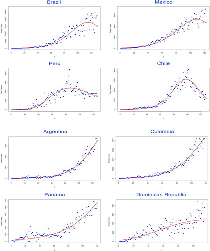
Figure 2. Fitting for the selected growth model by countries. The fitted growth curve (solid) and the actual number (dotted) of daily confirmed cases over the ordered days of the outbreak (II).

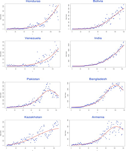
Figure 3. Fitting for the selected growth model by countries. The fitted growth curve (solid) and the actual number (dotted) of daily confirmed cases over the ordered days of the outbreak (III).

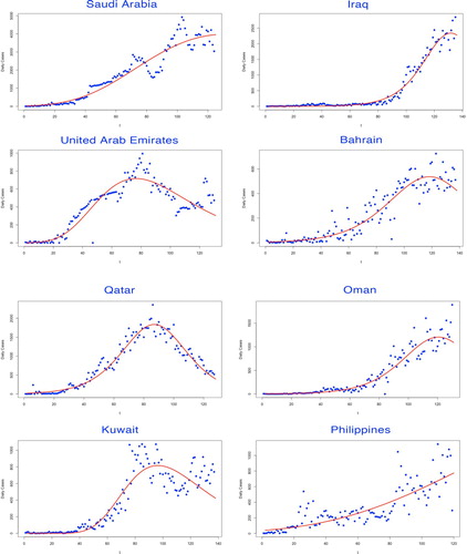
Figure 4. Fitting for the selected growth model by countries. The fitted growth curve (solid) and the actual number (dotted) of daily confirmed cases over the ordered days of the outbreak (IV).

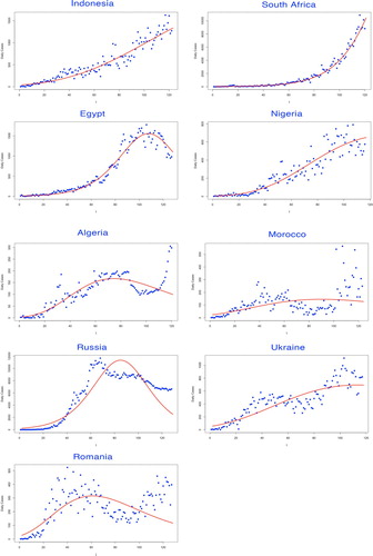
The selected growth model to determine the intrinsic growth rate r was judged by various evaluation criteria. The model with the lowest AIC and BIC values was considered as the best-fitted decision, leading to the estimate of r (see Table 2).

Table 2. Parameters of growth models for estimating basic reproduction number.

Countries	Model	$R^2$	AIC	BIC	r
Brazil	Logistic	0.9998	2692.09	2703.56	0.1600
Mexico	Logistic	0.9999	1912.69	1923.84	0.1514
Peru	Gompertz	0.9994	2354.36	2365.71	0.1753
Chile	Logistic	0.9974	2584.41	2595.85	0.0976
Argentina	Logistic	0.9961	2367.22	2391.62	0.1308
Colombia	Logistic	0.9996	2333.62	2343.79	0.1249
Panama	Logistic	0.9966	2343.83	2366.07	0.1204
Dominican Republic	Gompertz	0.9968	1795.71	1806.72	0.1304
Honduras	Logistic	0.9790	2482.94	2490.42	0.1292
Bolivia	Gompertz	0.9998	1602.32	1613.50	0.1243
Venezuela	Richards	0.9961	1391.08	1401.99	0.0891
India	Gompertz	0.9998	2304.74	2316.05	0.1754
Pakistan	Logistic	0.9957	2514.15	2525.50	0.1511
Bangladesh	Logistic	0.9996	1985.59	1996.68	0.1795
Kazakhstan	Richards	0.9980	1697.99	1708.79	0.1224
Armenia	Logistic	0.9983	1795.25	1806.43	0.1335
Saudi Arabia	Richards	0.9987	2306.45	2317.77	0.1640
Iraq	Logistic	0.9963	2244.70	2256.29	0.1450
United Arab Emirates	Gompertz	0.9992	2017.57	2029.069	0.1216
Bahrain	Logistic	0.9994	1883.66	1895.34	0.1056
Qatar	Logistic	0.9990	2181.65	2193.05	0.1098
Oman	Logistic	0.9990	1993.57	2005.07	0.1056
Kuwait	Richards	0.9981	2234.13	2245.84	0.0862
Philippines	Richards	0.9944	1958.55	1969.70	0.1119
Indonesia	Gompertz	0.9988	1953.95	1965.20	0.1300
South Africa	Logistic	0.9810	2015.26	2038.33	0.1602
Egypt	Logistic	0.9980	2164.77	2176.18	0.1318
Nigeria	Gompertz	0.9991	1664.38	1675.43	0.1677
Algeria	Gompertz	0.9985	1592.98	1604.16	0.1337
Morocco	Gompertz	0.9708	1999.16	2010.44	0.0879
Russia	Logistic	0.9993	2631.52	2642.96	0.2123
Ukraine	Gompertz	0.9934	2029.83	2040.91	0.0844
Romania	Gompertz	0.9891	2130.86	2142.27	0.0659

Results showed that the basic reproduction number $R_0$ of the studied 33 countries ranged from 1.60 (of Romania) to 3.28 (of Bangladesh) with a mean of 2.48 and a median of 2.43 approximately (see Table 1).

4.2. Estimation of infectious period $T_I$

In the second part of the modelling framework, the best-fitted $T_I$ was determined by the lowest prediction error through a complex statistical model given by Lin et al. (2020), which was built on the Poisson-distributed increment and shown in Figures 5–8.

Figure 5. Prediction error versus infectious period by countries (I).

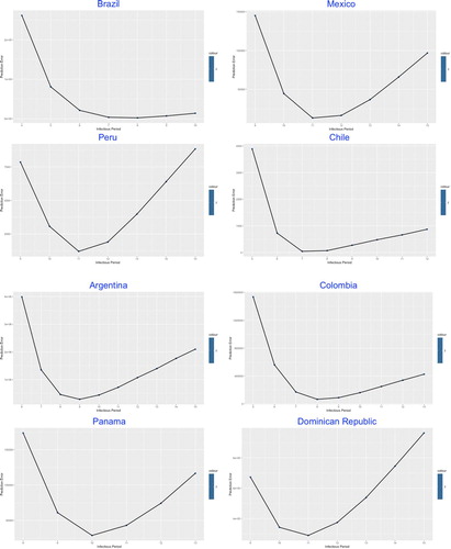
Figure 6. Prediction error versus infectious period by countries (II).

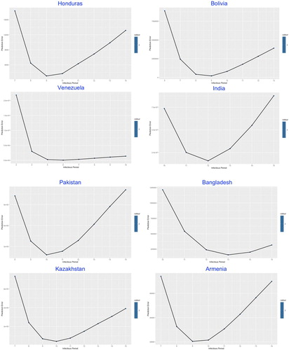
Figure 7. Prediction error versus infectious period by countries (III).

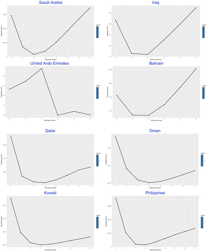
Figure 8. Prediction error versus infectious period by countries (IV).

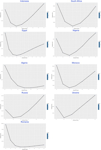
The similarity was demonstrated among most of the studied countries with common V-shaped line trend for the relation between prediction error and $T_I$, indicating the optimal number of the infectious period which stay at the trough.

The values of $T_I$ in Table 1, ranging from 5 (of Venezuela) to 13 (of Bangladesh and UAE) days, reflects the estimated average duration of infectious period, which in practice could be significantly shortened by intervention measures such as nationwide lockdown, social distancing, earlier population-based testing and self-isolation.

4.3. SIR-X model fitting

After implementing the calibrated model based on the $R_0$ and $T_I$ determined in the previous two sections, we then move on to the SIR-X dynamic model for achieving an explanatory prediction result for the potential development of epidemics. During the numerical approximation procedure, a fourth-order Runge–Kutta method was applied for the fitting of parameters. Using the mid-year population sizes N which were collected from official websites of the United Nations (https://population.un.org), we obtained the specific values for key modelling parameters ${\kappa }_0$, κ and ${\varphi }_0$, shown in Table 3, along with α and β which denoted the transmissibility and recovery rate. The fitting curves for the corresponding study periods generally fell close to the observed trajectories, which suggested a relatively effective model fitting performance (see Figures 9–12).

Figure 9. SIR-X model fitting by countries. The fitted growth curve (red-solid, smooth) and the actual growth curve (blue-solid, discretised) of daily confirmed cases over the ongoing dates of the outbreak. The predicted trajectory (green-solid) forecasts the daily growth of 100 days after the end of the study period (I).

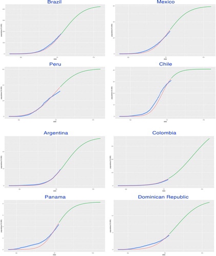
Figure 10. SIR-X model fitting by countries. The fitted growth curve (red-solid, smooth) and the actual growth curve (blue-solid, discretised) of daily confirmed cases over the ongoing dates of the outbreak. The predicted trajectory (green-solid) forecasts the daily growth of 100 days after the end of the study period (II).

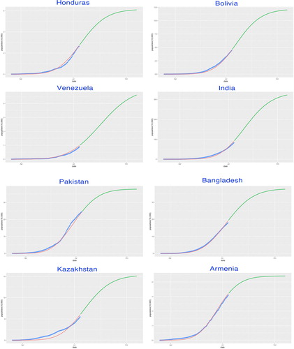
Figure 11. SIR-X model fitting by countries. The fitted growth curve (red-solid, smooth) and the actual growth curve (blue-solid, discretised) of daily confirmed cases over the ongoing dates of the outbreak. The predicted trajectory (green-solid) forecasts the daily growth of 100 days after the end of the study period (III).

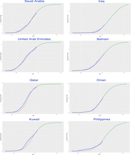
Figure 12. SIR-X model fitting by countries. The fitted growth curve (red-solid, smooth) and the actual growth curve (blue-solid, discretised) of daily confirmed cases over the ongoing dates of the outbreak. The predicted trajectory (green-solid) forecasts the daily growth of 100 days after the end of the study period (IV).

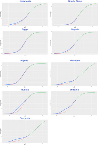
Table 3. Parameters of model SIR-X.

Countries	N	${\kappa }_0$	κ	${\mathrm{\Phi }}_0$	P	Q
Brazil	$2.1264\times {10}^8$	0.00312	0.19693	25.93271	0.01561	0.64292
Mexico	$1.2901\times {10}^8$	0.00717	0.00507	32.91247	0.58586	0.11859
Peru	$3.2995\times {10}^7$	0.00232	0.12683	152.78813	0.01800	0.58690
Chile	$1.9125\times {10}^7$	0.00298	0.00606	56.38177	0.32937	0.05953
Argentina	$4.5195\times {10}^7$	0.00519	0.00549	9.06407	0.48594	0.08765
Colombia	$5.0880\times {10}^7$	0.00125	0.10034	22.17644	0.01232	0.44834
Panama	$4.3140\times {10}^6$	0.00400	0.00231	5.16581	0.63415	0.05927
Dominican Republic	$1.0848\times {10}^7$	0.00380	0.02827	26.59146	0.11841	0.26076
Honduras	$9.9040\times {10}^6$	0.00597	0.00722	6.88260	0.45292	0.10611
Bolivia	$1.1673\times {10}^7$	0.00496	0.00537	11.26898	0.48019	0.08512
Venezuela	$2.8431\times {10}^7$	0.00179	0.08095	3.16287	0.02166	0.29263
India	$1.3800\times {10}^9$	0.00689	0.00110	20.59769	0.86268	0.08743
Pakistan	$2.2089\times {10}^8$	0.00774	0.00865	21.85809	0.47220	0.14088
Bangladesh	$1.6469\times {10}^8$	0.00850	0.00934	24.84376	0.47651	0.18832
Kazakhstan	$1.8776\times {10}^7$	0.00524	0.00211	18.19945	0.71284	0.06850
Armenia	$2.9630\times {10}^6$	0.00659	0.00876	5.07250	0.42926	0.12131
Saudi Arabia	$3.4842\times {10}^7$	0.00556	0.05787	17.94944	0.08763	0.38811
Iraq	$4.0266\times {10}^7$	0.00506	0.00396	5.28374	0.56096	0.09769
U.A.E	$9.8960\times {10}^7$	0.00748	0.00317	87.47645	0.70228	0.12165
Bahrain	$1.7040\times {10}^7$	0.00296	0.00682	43.45895	0.30275	0.10505
Qatar	$2.8830\times {10}^7$	0.00178	0.00640	27.96857	0.21754	0.06856
Oman	$5.1120\times {10}^6$	0.00361	0.00739	12.72974	0.32826	0.09013
Kuwait	$4.2730\times {10}^6$	0.00294	0.00842	15.24312	0.25883	0.07369
Philippines	$1.0966\times {10}^8$	0.00498	0.00561	13.24814	0.47002	0.07812
Indonesia	$2.7368\times {10}^8$	0.00605	0.00709	24.92229	0.46062	0.11613
South Africa	$5.9308\times {10}^7$	0.00612	0.00073	11.86611	0.89374	0.07599
Egypt	$1.0233\times {10}^8$	0.00754	0.00801	16.31997	0.48470	0.11065
Nigeria	$2.0638\times {10}^8$	0.00871	0.00761	8.23676	0.53379	0.15218
Algeria	$4.3890\times {10}^7$	0.00191	0.09209	8.91648	0.02027	0.45826
Morocco	$3.6910\times {10}^7$	0.00181	0.04686	57.28348	0.03728	0.28026
Russia	$1.4593\times {10}^8$	0.00312	0.19693	25.93271	0.01561	0.64292
Ukraine	$4.3717\times {10}^7$	0.00481	0.00998	71.79411	0.32516	0.08153
Romania	$1.9229\times {10}^7$	0.00112	0.03947	127.18860	0.02769	0.22127

Assuming the sustainability of intervention measures, the values of P and Q, also shown in Table 3, which are derived from the three estimated parameters ${\kappa }_0$, κ and β, quantify the public containment leverage and quarantine probability, respectively. Under most circumstances, higher public containment leverages leads to the substantial concordance with pure algebraic growth.

Appropriately, the SIR-X model was structurally consistent with respect to these parameters, while highlighting a sub-exponential scaling law as the balance between transmission and containment before the saturation of the case counts due to the decay of unidentified infecteds.

4.4. Estimation of the peak and plateau

In this study, the turning point of the first wave of a certain COVID-19 outbreak was defined as the date when the cumulative case number numerically reached the plateau which satisfies $|\frac{\mathrm{\partial }f\left(v\right)}{\mathrm{\partial }v}|⩽c_0$ where the ratio of increment is defined as $f\left(v\right)=\left[\frac{\mathrm{\partial }C\left(t\right)}{\mathrm{\partial }t}{|}_{t=v}\right]/\left[\frac{\mathrm{\partial }C\left(t\right)}{\mathrm{\partial }t}{|}_{t=v-1}\right]$ and $c_0$ is a prespecified small number. Here, we take $c_0=5\times {10}^{-4}$ (see Lin et al., 2020), and judge the exact date of the plateau only if the daily confirmed case numbers of all the following days satisfying this criterion.

Besides, the unidentified infectious compartment‘I’ distinguished the timing of the peak when the most infectious cases emerged. Note that the exact value of unidentified infecteds is sensitive to parameter changing, especially the population size N. However, the general shape of $I\left(t\right)$ remains consistent to be a Bell curve whose exponential decay right after the peak induces the saturation of the cumulative case number to a finite level.

From Table 1, conclusions about the predicted epidemic trends could therefore be drawn explicitly. Among 33 studied countries, the peaks were observed in 11 countries (with the earliest peak of UAE on the 13rd of May, 2020) and 15 countries before August, while the latest peak (of Colombia) is the 8th of September, 2020. Meanwhile, the timing of plateau exhibited that the first wave of epidemic would come into break around late August to September across the majority of the studied countries. Remarkably, under the current fitted parameters with the continuity of containment measures, the durations of fading, counted from the peak to the plateau, were mostly longer than one month. The difference of fading durations might partially reveal the significant effect of divergent containment measures implemented for various countries.

Specifically, in Asia, the epidemic will mostly continue until the end of August. India, Pakistan and Saudi Arabia, along with the Philippines, were expected to reach the plateau in September. With the second-largest population in the world, India has undoubtedly become the epicentre in Asia and was estimated to have a final size over 3.2 million cumulative confirmed cases by the ending date (19 October 2020) of our prediction.

In Latin America, the epidemic will fade out not before the second half of August, except for Peru and Chile whose turning points will emerge in early August. Among them, Brazil has the largest estimated infections with more than 4.2 million positive cases, which accounts for almost 2% of the nationwide population.

In the three studied European countries, both Russia and Ukraine have passed through the peak in late June and the plateau would be approached within this August. Moreover, Russia will achieve a final epidemic size of over 1 million confirmed infected cases. In addition, Romania was estimated to have a late climax a few days before September and the epidemic would last until the second half of September.

Though the substantial shortage of medical testing condition has greatly influence the validity of the statistics in Africa, it is no doubt that Africa has already become one of the non-negligible epicentre suffering from COVID-19. Among the five studied African countries, most of them would reach the plateau after September with the exception of Algeria, whose comparatively smooth trajectory would lead to the turning point at 18 August 2020. From our prediction, Morocco would hold the latest peak at 14 August 2020, while South Africa was expected to have the largest final size of nearly 700 thousand.

5. Conclusions and discussions

In this study, we focus on conducting analytical assessment and prediction on the degree of the epidemic outbreak across the currently developing epicentres. Considering the commonplace that when a brand new contagion starts evolving into the outbreak, there exists deficiency of public health related information, leaving only the reported cases available for academic research. Thus, we propose an integrated framework for analysing the COVID-19 time series cases, which were reported from 15 February 2020 to 10 July 2020. We track, evaluate and forecast the epidemic by comparative study of the epidemiological parameters and estimating the number of cumulative cases across various countries, assessing the impact of containment strategies, which should be constructive in mitigation planning and redeployment of resources.

The modelling framework has demonstrated adaptiveness and consistency on portraying epidemic trends across the studied countries, which is advisable for the quantitative analysis of the transmission mechanism of COVID-19, together with the implementation of control measures in current epicentres and for potential future outbreaks worldwide.

In summary, using the data from the first stage of the epidemic, our study provided a concrete modelling framework for estimation of the epidemiological parameters and prediction of future trajectories as well as explanatory features including the peak, the plateau and the final epidemic size of the current epicentres. Results of prediction were mostly considered as consistent with the observed growth curves. Meanwhile, we highlighted the importance of effective containment policies and quarantine measures in flattening the epidemic curves.

Fitted by the empirical case counts, the modelling framework generates the basic reproduction number $R_0$ and the infectious period $T_I$ catering for each country through typical epidemic growth models and a parsimonious statistical approach respectively. Plausible parameter values were well archived in most of our studied countries, indicating decent results obtained for the following modelling procedure of the dynamics.

Thus, the reproduced epidemic trajectories of the 33 studied countries could be applied to estimate the trend of the number of asymptomatic infected individuals, which is the key quantity for estimating the peak time of the outbreak.

The SIR-X model discussed here unveils that the remarkable feature to better depict the dynamics of the COVID-19 outbreaks in 33 studied countries is the sub-exponential scaling law in the growth of positive case numbers during the first wave of the epidemic. This common behaviour demonstrates that fundamental principles are practically correlated with the epidemic that are manipulated by the coaction of internal behavioural changes in the susceptibles as well as external containment policies and quarantine measures.

Despite the explanatory modelling performance, our study has several limitations. First of all, high reliance on the quality of data collection always remains a realistic constraint for most of the modelling study. The under-reporting of infection, the delay of testing feedback and the bandwidth of update in statistics are commonplace in a vast majority of countries. Even under such circumstances, our model framework has still been proved to accomplish the analysis with credible results including the dynamics and the predictions of final epidemic size, the peak and the plateau.

Secondly, during the process for estimating the basic reproduction number $R_0$, we directly applied the result of serial interval from a former study of Li et al. (2020), which was considered as a general alternative in consequence of lacking in the specific onset data from each studied country. We believe that the estimation of the basic reproduction number $R_0$ for each country will become more reliable with the support of its onset data that will lead to a precise assessment of the serial interval.

Thirdly, according to the setting of the statistical modelling in Section 3.2, the infectious period $T_I$ could only be achieved as a positive integer. Though more interpretable in practice, the neglect of numerical smoothness might restrict the parameter space for tuning of the SIR-X dynamic model, which would concern the accuracy for prediction.

Additionally, in the part of the SIR-X model, we simply assumed that the containment rate ${\kappa }_0$ and the quarantine rate κ are constant considering the fundamentality of data. In practice, the intervention strategies in a certain country would probably change dramatically for different epidemic stages, resulting in the time-varying containment and quarantine rate which remain the modification for further research.

Last but not least, as is shown in the results, the saturation of confirmed cases informs that eventually all susceptibles will ideally fall into the removal from the epidemic transmission process assuming that the containment and quarantine measures could be held on to the end of the epidemic for an extended period of time. However, a considerable number of susceptibles will not be quarantined as the consequence of either the ignorance of intervention policies or the shortage of quarantine space and testing resources. Indeed, the number of daily new cases expected will decline following a slower path and finally saturate to a comparatively small, yet non-zero level instead. Advisably, aiming to thoroughly cease the epidemic transmission, it would be worthy to extend statistics for unidentified and unquarantined infecteds. As a result, we expect that our predictions will partly underestimate the final epidemic sizes for studied countries.

Though generally well-fitted, there are still some of the studied countries, such as the last four studied countries (Morocco, Russia, Ukraine and Romania), whose goodness-of-fit seems rather poor. One of the potential reasons is that these countries have already entered the second wave of the epidemic trajectories, which will certainly not be suitable for our single wave model. The extension could be considered in further research so that our modelling framework will be adaptive to the second wave. With the complete empirical time-series data for the first epidemic wave, an accurate estimation for the reproduction number will be carried out. Moreover, due to the accumulated experience for the policy-making of containment, it is most likely that the infectious period of the second wave will be modified with more complexity, as well as different sets of transmission rates α and recovery rates β for the SIR-X dynamic models. With increasing data collected, it will be practical to develop piecewise modelling according to different stages of policy implementation period, resulting in the multiple sets of parameters ${\kappa }_0$ and κ.

The major difference between the modelling of the early epidemic and the second wave trajectories will be the initialisation, since the starting cases will remain non-negligible quantities on the basis of unidentified infected individuals that we've estimated. Thus, an adequate recognition of the initial point for launching the second wave will bring substantial influence on the prediction of trajectories.

It is generally believed that the second wave inclines to have a more extensive exponential rise to a higher peak which will probably last longer in a consequence of the hidden population of unidentified infected individuals and the relatively loosened containment policies implemented throughout the world. The upcoming vaccine will become another important factor that will affect the trajectories of some countries. Under such complicated circumstances, multi-wave modelling requires to be specifically validated by our future research based on the current modelling framework.

Disclosure statement

No potential conflict of interest was reported by the author(s).

Additional information

Funding

The research is supported by the Natural Science Foundation of China [Grant Numbers 11271136, 81530086] and the "Project 111" No. B14019 of China.

References

- Akaike, H. (1973). Information theory and an extension of the maximum likelihood principle (pp. 267–281). Akadémiai Kiadó.
- Ball, F., & Clancy, D. (1993). The final size and severity of a generalised stochastic multitype epidemic model. Advances in Applied Probability, 25(4), 721–736. https://doi.org/https://doi.org/10.2307/1427788
- Becker, N. (1977). On a general stochastic epidemic model. Theoretical Population Biology, 11(1), 23–36. https://doi.org/https://doi.org/10.1016/0040-5809(77)90004-1
- Becker, N., & Britton, T. (1999). Statistical studies of infectious disease incidence. Journal of the Royal Statistical Society: Series B, 61(2), 287–307. https://doi.org/https://doi.org/10.1111/rssb.1999.61.issue-2
- Chen, Y. C., Lu, P. E., Chang, C. S., & Liu, T. H. (2020). A time-dependent SIR model for COVID-19 with undetectable infected persons. IEEE Transactions on Network Science and Engineering, 7(4), 3279–3294. https://doi.org/10.1109/TNSE.2020.3024723
- Cleveland, W. S., & Devlin, S. J. (1988). Locally weighted regression: An approach to regression analysis by local fitting. Journal of the American Statistical Association, 83(403), 596–610. https://doi.org/https://doi.org/10.1080/01621459.1988.10478639
- Gompertz, B. (1825). On the nature of the function expressive of the law of human mortality, and on a new mode of determining the value of life contingencies. Philosophical Transactions of the Royal Society of London B: Biological Sciences, 115, 513–583. https://doi.org/https://doi.org/10.1098/rstl.1825.0026
- González, R. E. R. (2020). Different scenarios in the dynamics of SARS-Cov-2 infection: An adapted ODE model. arXiv:2004.01295. https://doi.org/10.21203/rs.3.rs–29563/v1.
- He, S., Peng, Y., & Sun, K. (2020). SEIR modeling of the COVID-19 and its dynamics. Nonlinear Dynamics, 101, 1667–1680. https://doi.org/https://doi.org/10.1007/s11071-020-05743-y
- Hethcote, H. W. (2000). The mathematics of infectious diseases. SIAM Review, 42(4), 599–653. https://doi.org/https://doi.org/10.1137/S0036144500371907
- Huang, N. E., Qiao, F., & Tung, K. K. (2020). A data-driven model for predicting the course of COVID-19 epidemic with applications for China, Korea, Italy, Germany, Spain. UK and USA. medRxiv e-prints. https://doi.org/10.1101/2020.03.28.20046177.
- Li, Q., Guan, X., Wu, P., Wang, X., Zhou, L., Tong, Y., Ren, R., Leung, K. S., Lau, E. H., Wong, J. Y., Xing, X., Xiang, N., Wu, Y., Li, C., Chen, Q., Li, D., Liu, T., Zhao, J., Liu, M., …Feng, Z. (2020). Early transmission dynamics in Wuhan, China, of novel coronavirus-infected pneumonia. The New England Journal of Medicine, 382, 1199–1207. https://doi.org/https://doi.org/10.1056/NEJMoa2001316
- Lin, H., Liu, W., Gao, H., Nie, J., & Fan, Q. (2020). Comparative analysis of early dynamic trends in novel coronavirus outbreak: A modeling framework. medRxiv e-prints. https://doi.org/10.1101/2020.02.21.20026468.
- Liu, C., Wu, X., Niu, R., Wu, X., & Fan, R. (2020). A new SAIR model on complex networks for analysing the 2019 novel coronavirus (COVID-19). Nonlinear Dynamics, 101, 1777–1787. https://doi.org/https://doi.org/10.1007/s11071-020-05704-5
- Maier, B. F., & Brockmann, D. (2020). Effective containment explains sub-exponential growth in confirmed cases of recent COVID-19 outbreak in Mainland China. Science, 368(6492), 742–746. https://doi.org/https://doi.org/10.1126/science.abb4557
- Mohamadou, Y., Halidou, A., & Kapen, P. T. (2020). A review of mathematical modeling, artificial intelligence and datasets used in the study, prediction and management of COVID-19. Applied Intelligence, 50, 3913–3925. https://doi.org/https://doi.org/10.1007/s10489-020-01770-9
- Peng, L., Yang, W., Zhang, D., Zhuge, C., & Hong, L. (2020). Epidemic analysis of COVID-19 in China by dynamical modeling. medRxiv e-prints. https://doi.org/10.1101/2020.02.16.20023465.
- Rajagopal, K., Hasanzadeh, N., Parastesh, F., Hamarash, I. I., Jafari, S., & Hussain, I. (2020). A fractional-order model for the novel coronavirus (COVID-19) outbreak. Nonlinear Dynamics, 101, 711–718. https://doi.org/https://doi.org/10.1007/s11071-020-05757-6
- Richards, F. J. (1959). A flexible growth function for empirical use. Journal of Experimental Botany, 10(2), 290–300. https://doi.org/https://doi.org/10.1093/jxb/10.2.290
- Schwarz, G. E. (1978). Estimating the dimension of a model. Annals of Statistics, 6(2), 461–464. https://doi.org/https://doi.org/10.1214/aos/1176344136
- Song, P. X., Wang, L., Zhou, Y., He, J., Zhu, B., Wang, F., Tang, L., & Eisenberg, M. (2020). An epidemiological forecast model and software assessing interventions on COVID-19 epidemic in China. medRxiv e-prints. https://doi.org/10.1101/2020.02.29.20029421.
- Sun, H., Qiu, Y., Yan, H., Huang, Y., Zhu, Y., & Chen, S. X. (2020). Tracking and predicting COVID-19 epidemic in China Mainland. medRxiv e-prints. https://doi.org/10.1101/2020.02.17.20024257.
- Tang, B., Wang, X., Li, Q., Bragazzi, N. L., Tang, S., Xiao, Y., & Wu, J. (2020). Estimation of the transmission risk of 2019-nCoV and its implication for public health interventions. Journal of Clinical Medicine, 9(2), 462. https://doi.org/https://doi.org/10.3390/jcm9020462
- Verhulst, P. F. (1838). Notice sur la loi que la population poursuit dans son accroissement. Correspondance Mathématique Et Physique, 10, 113–121.
- Wallinga, J., & Lipsitch, M. (2007). How generation intervals shape the relationship between growth rates and reproductive numbers. Proceedings of the Royal Society B: Biological Sciences, 274, 599–604. https://doi.org/https://doi.org/10.1098/rspb.2006.3754
- Wang, X., Wang, S., Lan, Y., Tao, X., & Xiao, J. (2020). The impact of asymptomatic individuals on the strength of public health interventions to prevent the second outbreak of COVID-19. Nonlinear Dynamics, 101, 2003–2012. https://doi.org/https://doi.org/10.1007/s11071-020-05736-x
- Wang, T., Wu, Y., Lau, J. Y. N., Yu, Y., Liu, L., Li, J., Zhang, K., Tong, W., & Jiang, B. (2020). A four-compartment model for the COVID-19 infection – implications on infection kinetics, control measures, and lockdown exit strategies. Precision Clinical Medicine, 3(2), 104–112. https://doi.org/https://doi.org/10.1093/pcmedi/pbaa018
- Wu, J. T., Leung, K., & Leung, G. M. (2020). Nowcasting and forecasting the potential domestic and international spread of the 2019-nCoV outbreak originating in Wuhan, China: A modelling study. The Lancet, 395(10225), 689–697. https://doi.org/https://doi.org/10.1016/S0140-6736(20)30260-9
- Xu, C., Yu, Y., Chen, Y., & Lu, Z. (2020). Forecast analysis of the epidemics trend of COVID-19 in the USA by a generalized fractional-order SEIR model. Nonlinear Dynamics, 101, 1621–1634. https://doi.org/https://doi.org/10.1007/s11071-020-05946-3
- Yang, Z., Zeng, Z., Wang, K., Wong, S. S., Liang, W., Zanin, M., Liu, P., Cao, X., Gao, Z., Mai, Z., Liang, J., Liu, X., Li, S., Li, Y., Ye, F., Guan, W., Yang, Y., Li, F., Luo, S., …He, J. (2020). Modified SEIR and AI prediction of the epidemics trend of COVID-19 in China under public health interventions. Journal of Thoracic Disease, 12(2), 165–174. https://doi.org/https://doi.org/10.21037/jtd
- Yip, P. S., & Chen, Q. (1998). Statistical inference for a multitype epidemic model. Journal of Statistical Planning and Inference, 71(1–2), 229–244. https://doi.org/https://doi.org/10.1016/S0378-3758(98)00087-1
- Zhao, S., Lin, Q., Ran, J., Musa, S. S., Yang, G., Wang, W., Lou, Y., Gao, D., Yang, L., He, D., & Wang, M. H. (2020). Preliminary estimation of the basic reproduction number of novel coronavirus (2019-nCoV) in China, from 2019 to 2020: A data-driven analysis in the early phase of the outbreak. International Journal of Infectious Diseases, 92, 214–217. https://doi.org/https://doi.org/10.1016/j.ijid.2020.01.050
- Zhao, S., Musa, S. S., Fu, H., He, D., & Qin, J. (2019). Simple framework for real-time forecast in a data-limited situation: The Zika virus (ZIKV) outbreaks in Brazil from 2015 to 2016 as an example. Parasites & Vectors, 12, 344. https://doi.org/https://doi.org/10.1186/s13071-019-3602-9