Covariance estimation via fiducial inference

Abstract

As a classical problem, covariance estimation has drawn much attention from the statistical community for decades. Much work has been done under the frequentist and Bayesian frameworks. Aiming to quantify the uncertainty of the estimators without having to choose a prior, we have developed a fiducial approach to the estimation of covariance matrix. Built upon the Fiducial Berstein–von Mises Theorem, we show that the fiducial distribution of the covariate matrix is consistent under our framework. Consequently, the samples generated from this fiducial distribution are good estimators to the true covariance matrix, which enable us to define a meaningful confidence region for the covariance matrix. Lastly, we also show that the fiducial approach can be a powerful tool for identifying clique structures in covariance matrices.

Keywords:

• covariance estimation
• sparsity
• fiducial inference
• cliques

2010 Mathematics Subject Classifications:

• Primary 62J10
• 62E20
• 62F25
• Secondary 62F12

1. Introduction

Estimating covariance matrices has historically been a challenging problem. Many regression-based methods have emerged in the last few decades, especially in the concept of ‘large p small n’. Among the notable methods, there are the graphical LASSO algorithms (Friedman et al., 2008, 2010; Rothman, 2012). Pourahmadi provided a detailed overview on the progress of covariance estimation (Pourahmadi, 2011). The Positive Definite Sparse Covariance Estimators (PDSCE) method (Rothman, 2012) has grained great popularity due to its performance comparing to other current methods, although it only produces a point estimator.

Aiming to have a distribution of good covariance estimators, we propose a generalised fiducial approach. The ideas underpinning fiducial inference were introduced by Fisher (1922,1930,1933,1935), whose intention was to overcome the need for priors and other issues with Bayesian methods perceived at the time. The procedure of fiducial inference allows to obtain a measure on the parameter space without requiring priors and defines approximate pivots for parameters of interest. It is ideal when a priori information about the parameters is unavailable. The key recipe of the fiducial argument is the data generating equation. Roughly, the generalised fiducial likelihood is defined as the distribution of the functional inverse of the data generating mechanism.

One great advantage of the fiducial approach to covariance matrix estimation is that, without specifying a prior, it produces a family of matrices that are close to the true covariance with a probabilistic characterisation using the fiducial likelihood function. This attractive property enables a meaningful definition for matrix confidence regions.

We are particularly interested in a high-dimensional multivariate linear model setting with possibly an atypical sparsity constraint. Instead of classical sparsity assumptions on the covariance matrix, we consider a type of experimental design that enforces sparsity on the covariate matrix. This phenomenon often arises in the studies of metabolomics and proteomics. One example of this setup is modelling the relationship between a set of gene expression levels and a list of metabolomic data. The expression levels of the genes serve as the predictor variables while the response variables are a variety of metabolite levels, such as sugar and triglycerides. It is known that only a small subset of genes contribute to each metabolite level, and each gene can be responsible for just a few metabolite levels.

Under the sparse covariate setting, we derive the generalised fiducial likelihood of the covariate matrix based on given observations and prove its asymptotic consistency as the sample size increases. For the covariance with community structures (cliques), we prove the necessary conditions for achieving accurate clique structure estimation. Samples from the fiducial distribution of a covariate matrix can be generated using Monte Carlo methods. In the general case, a reversible jump Markov chain Monte Carlo (RJMCMC) algorithm may be needed. Similar to the classic likelihood functions, fiducial distributions favour models with more parameters. Therefore, in the case where the exact sparsity structure of the covariate is unclear, a penalty term needs to be added. To obtain a family of covariance estimators in the general case, we adapt a zeroth-order method and develop an efficient RJMCMC algorithm that samples from the penalised fiducial distribution.

The rest of the paper is arranged as follows. In Section 2, we will provide a brief background and development on fiducial inference. Then we will introduce the fiducial model for covariance estimation and derive the Generalised Fiducial Distribution (GFD) for the covariate and covariance matrices and examine the asymptotic property of the GFD of the covariance matrix under minor assumptions in Section 3. Some toy examples on sampling from GFD will also be shown. Section 4 focuses on the clique model, where we show some theoretical results for the clique model and how the fiducial approach can be applied to uncover clique structures. Finally, Section 5 concludes the paper with a summary and a short discussion on the relationship of our approach to Bayesian methods.

2. Generalised fiducial inference

2.1. Brief background

Fiducial inference was first proposed by Fisher (1930) when he introduced the concept of a fiducial distribution of a parameter. In the case of a single parameter family of distributions, Fisher gave the following definition for a fiducial density $f\left(\theta |x\right)$ of the parameter based on a single observation x for the case where the cumulative distribution function $F\left(x|\theta \right)$ is a monotonic decreasing function of θ: (1) $\begin{array}{r}f\left(\theta |x\right)\propto -\frac{\mathrm{\partial }F\left(x|\theta \right)}{\mathrm{\partial }\theta }.\end{array}$(1) A fiducial distribution can be viewed as a Bayesian posterior distribution without hand picking priors. In many single parameter distribution families, Fisher's fiducial intervals coincide with classical confidence interval. For families of distributions with multiple parameters, the fiducial approach leads to confidence set. The definition of fiducial inference has been generalised in the past decades. Hannig et al. (2016) provide a detailed review on the philosophy and current development on the subject.

The generalised fiducial approach has been applied to a variety of models, both parametric and nonparametric, both continuous and discrete. These applications include bioequivalence (Hannig et al., 2006), variance components (Cisewski & Hannig, 2012; Lidong et al., 2008; Li et al., 2018), problems of metrology (Hannig et al., 2007,2003; Wang et al., 2012; Wang & Iyer, 2005, 2006a, 2006b), inter laboratory experiments and international key comparison experiments (Hannig et al., 2018; Iyer et al., 2004), maximum mean of a multivariate normal distribution (Wandler & Hannig, 2011), multiple comparisons (Wandler & Hannig, 2012), extreme value estimation (Wandler & Hannig, 2012), mixture of normal and Cauchy distributions (Glagovskiy, 2006), wavelet regression (Hannig & Lee, 2009), high-dimensional regression (Lai et al., 2015; Williams & Hannig, 2018), item response models (Liu & Hannig, 2016,2017), non-parametric survival function estimation with censoring (Cui & Hannig, 2019), Other related approaches include Martin and Liu (2015); Schweder and Hjort (2016); Xie and Singh (2013).

2.2. Generalised fiducial distribution

The idea underlying generalised fiducial inference is built upon a data generating algorithm $G(\cdot ,\cdot )$ expressing the relationship between the data X and the parameters θ: (2) $\begin{array}{r}X=G(U,\theta ),\end{array}$(2) where U is the random component of this data generating algorithm whose distribution is known. The data X are assumed to be created by generating a random variable U and plugging it into the data generating algorithm above.

The GFD inverts Equation (2(2) $\begin{array}{r}X=G(U,\theta ),\end{array}$(2) ). Assume that $x\in {\mathbb{R}}^n$ is continuous, and the parameter $\theta \in {\mathbb{R}}^p$. Under the conditions provided in Hannig et al. (2016), fiducial distribution is shown to have density (3) $\begin{array}{r}r\left(\theta |x\right)=\frac{f(x,\theta )J(x,\theta )}{{\displaystyle {\int }_{\mathrm{\Theta }}f(x,{\theta }^{\prime })J(x,{\theta }^{\prime })\mathrm{d}{\theta }^{\prime }}},\end{array}$(3) where $f(x,\theta )$ is the likelihood, and (4) $\begin{array}{r}J(x,\theta )=D\left({\left.{\mathrm{\nabla }}_{\theta }G(u,\theta )\right|}_{u=G^{-1}(x,\theta )}\right).\end{array}$(4) Here ${\mathrm{\nabla }}_{\theta }G(u,\theta )$ is the $n\times p$ Jacobian matrix. The exact form of $D(\cdot )$ depends on the choices made in the process of inverting (2(2) $\begin{array}{r}X=G(U,\theta ),\end{array}$(2) ). In this manuscript, we concentrate on what Hannig et al. (2016) calls the ${\ell }_2$-norm choice: (5) $\begin{array}{r}D\left(M\right)=\sqrt{\text{det}\left(M^{\mathrm{T}}M/n\right)},\end{array}$(5) where $M^{\mathrm{T}}$ denotes the matrix transpose of M. Other choices, in particular the ${\ell }_{\mathrm{\infty }}$-norm that was often used in the past, leads to similar results is studied in detail in Shi (2015).

3. A fiducial approach to covariance estimation

In this section, we will derive the GFD for the covariance matrix of a multivariate normal random variable. For this problem, various regularised estimators were proposed under the assumption that the true covariance matrix is sparse (Avella-Medina et al., 2018; Bickel & Levina, 2008a, 2008b; Cai & Liu, 2011; Furrer & Bengtsson, 2007; Huang & Lee, 2016; Huang et al., 2006; Lam & Fan, 2009; Levina et al., 2008; Rothman et al., 2009, 2010; Wu & Pourahmadi, 2003). While many of these estimators have been shown to enjoy excellent rates of convergence, so far little work has been done to quantify the uncertainties of their corresponding estimates.

Let $Q^{\mathrm{T}}$ denote the transpose of a matrix/vector Q. Denote a collection of n observed p dimensional objects $\mathbf{Y}=\{Y_i:i=1,\dots ,n\}$. For the rest of the paper, we assume p is fixed, unless stated otherwise. Consider the following data generating equation: (6) $\begin{array}{r}{Y}_i=A{Z}_i,i=1,\dots ,n;\end{array}$(6) where A is a $p\times p$ matrix of full rank; $\mathit{Z}=\{Z_i=(z_{i1},\dots ,z_{ip}{)}^{\mathrm{T}},i=1,\dots ,n\}$ are independent and identically distributed (i.i.d) $p\times 1$ random vectors following multivariate normal distribution $N(0,I)$. Hence, $Y_i$'s are i.i.d random vectors centred at 0 with covariance matrix $A{A}^{\mathrm{T}}$, (7) $\begin{array}{r}\mathrm{i}.\mathrm{e}.Y_i\stackrel{\mathrm{i}.\mathrm{i}.\mathrm{d}}{\sim }N(0,\mathrm{\Sigma }),\mathrm{w}\mathrm{h}\mathrm{e}\mathrm{r}\mathrm{e}\mathrm{\Sigma }=A{A}^{\mathrm{T}}.\end{array}$(7) Consequently, we have the likelihood for observations $\mathit{y}$: (8) $\begin{array}{rl}f(\mathit{y},A)& =\left(2\text{π}{)}^{-\frac{np}{2}}|\text{det}\right(A){|}^{-n}\\ & \times \exp \left[-\frac{1}{2}\text{tr}\left\{n{S}_n\right(A{A}^{\mathrm{T}}{)}^{-1}\}\right],\end{array}$(8) where $S_n=\frac{1}{n}\sum _{i=1}^n{y}_i{y}_i^{\mathrm{T}}$ is the corresponding sample covariance matrix and $\text{tr}\{\cdot \}$ is the trace operator.

We propose to estimate the covariance matrix Σ through the GFD of covariate matrix A: (9) $\begin{array}{r}r\left(A|\mathit{y}\right)\propto J(\mathit{y},A)f(\mathit{y},A).\end{array}$(9) Define the stacked observation vector $\mathbf{w}=(y_1^{\mathrm{T}},\dots ,y_n^{\mathrm{T}}{)}^{\mathrm{T}}=(w_1,\dots ,w_{np}{)}^{\mathrm{T}}$. Denote $\mathbf{u}=(u_1,\dots ,u_n)$, such that $y_i=G(u_i,A),\mathrm{\forall }i$. Let $a_{ij}$ be the $(i,j)$-th entry of matrix A, i.e., $A=[a_{ij}{]}_{1\le i,j\le p}$. The corresponding Jacobian $J(\mathit{y},A)$ derived from (4(4) $\begin{array}{r}J(x,\theta )=D\left({\left.{\mathrm{\nabla }}_{\theta }G(u,\theta )\right|}_{u=G^{-1}(x,\theta )}\right).\end{array}$(4) ) is then (10) $\begin{array}{r}J(\mathit{y},A)=D\left({\left.{\mathrm{\nabla }}_A\mathbf{w}\right|}_{\mathbf{u}=G^{-1}(\mathit{y},A)}\right),\end{array}$(10) where ${\mathrm{\nabla }}_A\mathbf{w}$ is an $np\times p^2$ matrix ${\mathrm{\nabla }}_A\mathbf{w}=\left(\begin{array}{cccc}\frac{\mathrm{\partial }{w}_1}{\mathrm{\partial }{a}_{11}}& \frac{\mathrm{\partial }{w}_1}{\mathrm{\partial }{a}_{12}}& \cdots & \frac{\mathrm{\partial }{w}_1}{\mathrm{\partial }{a}_{pp}}\\ \frac{\mathrm{\partial }{w}_2}{\mathrm{\partial }{a}_{11}}& \frac{\mathrm{\partial }{w}_2}{\mathrm{\partial }{a}_{12}}& \cdots & \frac{\mathrm{\partial }{w}_2}{\mathrm{\partial }{a}_{pp}}\\ ⋮& ⋮& \ddots & ⋮\\ \frac{\mathrm{\partial }{w}_{np}}{\mathrm{\partial }{a}_{11}}& \frac{\mathrm{\partial }{w}_{np}}{\mathrm{\partial }{a}_{12}}& \cdots & \frac{\mathrm{\partial }{w}_{np}}{\mathrm{\partial }{a}_{pp}}\end{array}\right)$and $D(\cdot )$ is given by (5(5) $\begin{array}{r}D\left(M\right)=\sqrt{\text{det}\left(M^{\mathrm{T}}M/n\right)},\end{array}$(5) ).

Often some $a_{kl}$ are known to be zero; a common example is the lower triangular matrix A for which $a_{kl}=0$ for l>k. Additionally, sparsity on the covariate model can be introduced by having most of the $a_{kl}$ known to be zero as a part of the model. Note that if $a_{kl}$ is known to be zero, as implied by model, then the corresponding $(k,l)$th column is dropped. Therefore, depending on the sparsity model, the dimension of ${\mathrm{\nabla }}_A\mathbf{w}$ varies.

Recall, that there is a one-to-one mapping between positive definite matrices Σ and lower triangular matrices A with positive entries on the main diagonal. While we are not assuming A is lower triangular, in order to alleviate some identifiability issues we will assume that all diagonal entries of A are positive, i.e., $a_{kk}>0,k=1,\dots ,p$.

3.1. Jacobian for full models

Suppose that none of the entries of A is fixed at zero, namely, the parameter space Θ for A is ${\mathbb{R}}^{p\times p}$. We will refer this to a full model. Under a full model, ${\mathrm{\nabla }}_A\mathbf{w}$ consists of p blocks, each of dimension $np\times p$. Every row of ${\mathrm{\nabla }}_A\mathbf{w}$ has non-zero entries in only one block.

By swapping rows in the matrix ${\mathrm{\nabla }}_A\mathbf{w}$ and plugging $\mathbf{u}=G^{-1}(\mathit{y},A)$, we obtain the $np\times p^2$ matrix P: (11) $\begin{array}{r}P=\left(\begin{array}{ccc}U& & \\ & \ddots & \\ & & U\end{array}\right),\end{array}$(11) where $U=(A^{-1}{y}_1,\cdots ,A^{-1}{y}_n{)}^{\mathrm{T}}=V(A^{-1}{)}^{\mathrm{T}},V=(y_1;\cdots ;y_n{)}^{\mathrm{T}}.$ Notice that P breaks into p blocks, $B_1,\dots ,B_p$, where $B_i=\left(\begin{array}{c}{O}_{(ni-n)\times p}\\ U\\ O_{(np-ni)\times p}\end{array}\right)$, $O_{a\times b}$ denotes a zero matrix with dimension $a\times b$.

Since as a consequence of Cauchy–Binnet formula (see also Hannig et al. (2016)), swapping rows do not change the value of the Jacobian function (10(10) $\begin{array}{r}J(\mathit{y},A)=D\left({\left.{\mathrm{\nabla }}_A\mathbf{w}\right|}_{\mathbf{u}=G^{-1}(\mathit{y},A)}\right),\end{array}$(10) ). Therefore $J(\mathit{y},A)$ can be expressed using matrix P: (12) $\begin{array}{r}J(\mathit{y},A)=D\left(P\right)={\left|\text{det}\left(S_n\right)\right|}^{\frac{p}{2}}|\text{det}\left(A\right){|}^{-p},\end{array}$(12) where $S_n=n^{-1}\sum _{i=1}^n{y}_i{y}_i^{\mathrm{T}}$ is the MLE estimator of the covariance matrix.

By (9(9) $\begin{array}{r}r\left(A|\mathit{y}\right)\propto J(\mathit{y},A)f(\mathit{y},A).\end{array}$(9) ), the GFD is proportional to (13) $\begin{array}{rl}r\left(A|\mathit{y}\right)& \propto {\left|\text{det}\left(S_n\right)\right|}^{\frac{p}{2}}\left(2\text{π}{)}^{-\frac{np}{2}}|\text{det}\right(A){|}^{-(n+p)}\\ & \times \exp \left[-\frac{1}{2}\text{tr}\left\{n{S}_n\right(A{A}^{\mathrm{T}}{)}^{-1}\}\right].\end{array}$(13) By transforming the GFD of A, we conclude that the GFD of $\mathrm{\Sigma }=A{A}^{\mathrm{T}}$ has the inverse Wishart distribution with n degrees of freedom and parameter $n{S}_n.$

3.2. Jacobian for the general case

While having a closed form for the GFD of Σ for the full model, the covariance estimation requires sufficient number of observations (roughly at least $n>15(p+1)$) to maintain reasonable power. In the cases where n is small, we reduce the parameter space by introducing a sparse structure $\mathcal{M}$, which determines which entries of A are known to be zero. Recall, that we only consider A with positive diagonal entries.

Now assume the general case with a sparse model $\mathcal{M}$, where some entries of A are known to be zero. Denote the $(i,j)$th entry of A as $A_{ij}$. Define the zero index set for the ith row as (14) $\begin{array}{r}{S}_i=\{j:A_{ij}\equiv 0,j=1,\dots ,p\},i=1,\dots ,p.\end{array}$(14) The set $S_i$ indicates which entries of A in the ith row are fixed at zero.

Then Equation (10(10) $\begin{array}{r}J(\mathit{y},A)=D\left({\left.{\mathrm{\nabla }}_A\mathbf{w}\right|}_{\mathbf{u}=G^{-1}(\mathit{y},A)}\right),\end{array}$(10) ) becomes (15) $\begin{array}{r}J(\mathit{y},A)=D\left(\tilde{P}\right),\end{array}$(15) where $\tilde{P}=({\tilde{B}}_1,\dots ,{\tilde{B}}_p)$ is the matrix P with correct corresponding columns dropped, i.e., block ${\tilde{B}}_i$ is obtained from block $B_i$ with $S_i$ columns removed.

Let $p_i$ be the number of nonzero entries in the ith row of A, and $U_i$ be the sub-matrix of U excluding columns in $S_i$, i.e., $U_i=U_{[:,-S_i]}$. Consequently, Equation (15(15) $\begin{array}{r}J(\mathit{y},A)=D\left(\tilde{P}\right),\end{array}$(15) ) becomes (16) $\begin{array}{r}J(\mathit{y},A)=\sqrt{\prod _i^p\text{det}\left(U_i^{\mathrm{T}}{U}_i/n\right)}.\end{array}$(16)

3.3. Consistency of fiducial distribution

In general, there is no one-to-one correspondence between the covariance matrix Σ and the covariate matrix A. However, if A is sparse enough, e.g., a lower triangular matrix with positive diagonal entries, the identifiability problem vanishes. In this section, we will show that, if there is one-to-one correspondence between Σ and A, then the GFD of the covariate matrix achieves a fiducial Bernstein–von Mises Theorem (Theorem 3.1), which provides theoretical guarantees of asymptotic normality and asymptotic efficiency for the GFD (Hannig et al., 2016).

The results here are derived based on FM-distance (Förstner & Moonen, 1999). For two symmetric positive definite matrices M and N, with the eigenvalues ${\lambda }_i(M,N)$ from $\text{det}(\lambda M-N)=0$, the FM-distance between the two matrices M and N is (17) $\begin{array}{r}\mathbf{d}(M,N)=\sqrt{\sum _{i=1}^n{\log }^2{\lambda }_i(M,N)}.\end{array}$(17) This distance measure is a metric and invariant with respect to both affine transformations of the coordinate system and an inversion of the matrices (Förstner & Moonen, 1999).

The Bernstein–von Mises Theorem provides conditions under which the Bayesian posterior distribution is asymptotically normal (van der Vaart, 1998; Ghosh & Ramamoorthi, 2003). The fiducial Bernstein–von Mises Theorem is an extension that includes a list of conditions under which the GFD is asymptotically normal (Sonderegger & Hannig, 2012). Those conditions can be divided into three parts to ensure each of the following:

1. the Maximum Likelihood Estimator (MLE) is asymptotically normal;

2. the Bayesian posterior distribution becomes close to that of the MLE;

3. the fiducial distribution is close to the Bayesian posterior.

It is clear that the MLE of Σ is asymptotically normal. Under our model, the conditions for (b) hold due to Proposition A.1 and the construction of the Jacobian formula; the conditions for (c) are satisfied by Propositions A.2, 3.1. Statements and proofs of the propositions are included in Appendix A.1. Here we state only Proposition 3.1 that contains notation needed in the statement of the main Theorem.

Proposition 3.1

The Jacobian function $J(\mathit{y},A)⟹\mathrm{a}.\mathrm{s}.{\pi }_{{\mathrm{\Sigma }}_0}\left(A\right)$ uniformly on compacts in A, where ${\pi }_{{\mathrm{\Sigma }}_0}\left(A\right)$ is a function of A, independent of the sample size and observations, but depending on the true ${\mathrm{\Sigma }}_0$. Moreover ${\pi }_{{\mathrm{\Sigma }}_0}\left(A\right)$ is continuous.

Closely following Sonderegger Hannig (2012), we arrive at Theorem 3.1.

Theorem 3.1

Asymptotic Normality

Let ${\mathcal{R}}_A$ be an vectorized observation from the fiducial distribution $r\left(A|\mathit{y}\right)$ and denote the density of $B=\sqrt{n}({\mathcal{R}}_A-{\hat{A}}_n)$ by ${\pi }^{\ast }(B,\mathit{y})$, where ${\hat{A}}_n$ is the vectorized version of a maximum likelihood estimator. Let $I\left(A\right)$ be the Fisher information matrix of the vectorized version of matrix (A). If the sparsity structure is such, that there is one-to-one correspondence between the true covariance matrix ${\mathrm{\Sigma }}_0$ and the covariate matrix $A_0$, $I\left(A_0\right)$ is positive definite, ${\pi }_{{\mathrm{\Sigma }}_0}\left(A_0\right)>0$, then (18) $\begin{array}{rl}& {\int }_{{\mathbb{R}}^{p^2}}\left|{\pi }^{\ast }(B,\mathit{y})-\frac{\sqrt{\mathrm{d}\mathrm{e}\mathrm{t}|I\left(A_0\right)|}}{(2\text{π}{)}^p}\right.\\ & \times \left.\exp \{-B^{\mathrm{T}}I(A_0\left)B/2\right\}\right|\mathrm{d}B⟹P_{A_0}0.\end{array}$(18)

See Appendix A.2 for the proof.

Remark 3.1

Since we assume that the diagonal entries of A are positive, the assumption of one-to-one correspondence between ${\mathrm{\Sigma }}_0$ and $A_0$ is satisfied if rows and columns of A can be permuted so that the resulting matrix is lower triangular matrix with positive entries on diagonal.

There are other highly sparse matrices for which there might be a finite number of different $A_{0,r}$ so that ${\mathrm{\Sigma }}_0=A_{0,r}{A}_{0,r}^{\mathrm{T}}$. Of course in this case we cannot distinguish between these $A_{0,r}$ based on data. However, Theorem 3.1 will still be true if we restrict the domain of A to a small enough Euclidean neighbourhood of any of the $A_{0,r}$. Each of these neighbourhoods being selected with a chance proportional to ${\pi }_{{\mathrm{\Sigma }}_0}\left(A_{0,r}\right)$.

3.4. Sampling in the general case

Given the true model ${\mathcal{M}}_0$, standard Markov chain Monte Carlo (MCMC) methods can be utilised for the estimation of the covariance matrix. Under the full model and clique model, the GFD of Σ follows either an inverse Wishart distribution or a composite of inverse Wishart distributions (see Section 3). Sampling from the GFD becomes straight forward and it can be done through one of the inverse Wishart random generation functions, e.g., InvWishart (MCMCpack, R) or iwishrnd (Matlab).

When p is small and n is large, the estimation of Σ can always be done through this setting, regardless if there are zero entries in A. The concept of having entries of A fixed at zero is to impose sparsity structure and allow estimation under a high dimensional setting without requiring large number of observations. As in practice the true sparse structure is often unobserved, we will focus on the cases where ${\mathcal{M}}_0$ is not given.

For the general case, if the sparse model is unknown, we propose to utilise a reversible jump MCMC (RJMCMC) method to efficiently sample from Equation  (20(20) $\begin{array}{rl}& r_p(A|\mathcal{M},\mathit{y})\propto r(A|\mathcal{M},\mathit{y})\\ & \times \exp \left\{-\sum _{i=1}^p\left[\frac{1}{2}{p}_i\log \left(np\right)+\log \left(\begin{array}{c}p\\ p_i\end{array}\right)\right]\right\}.\end{array}$(20) ) and simultaneously update $\mathcal{M}$.

RJMCMC is an extension of standard Markov chain Monte Carlo methods that allows simulation of the target distribution on spaces of varying dimensions (Green, 1995). The ‘jumps’ refers to moves between models with possibly different parameter spaces. More details on RJMCMC can be found in Shi (2015). Since $\mathcal{M}$ is unknown, namely the number and the locations of fixed zeros in the matrix A are unknown, the property of jumping between parameter spaces with different dimension is desired for estimating $\mathrm{\Sigma }=A{A}^{\mathrm{T}}$. Because the search space for RJMCMC is both within parameter space and between spaces, it is known for slower convergence. To improve efficiency of the algorithm, we adapt the zeroth-order method (Brooks et al., 2003) and impose additional sparse constrains.

Assuming that there are fixed zeros in A, then for a $p\times p$ matrix A, the number needed to be estimated is less than $p^2$. If there are many fixed zeros, then this number is much smaller, hence the estimation is feasible even if the number of observations n is less than p. In other words, the sparsity assumption on A allows estimations under a large p small n setting. Suppose the zero entry locations of A are known. The rest of A can be obtain via standard MCMC techniques, such as Metropolis–Hastings.

Figure 1 considers a case with $p=15,n=30$. It shows the confidence curve plot per Markov chain for each statistic of interest. In addition to D2Sig, LogD and Eigvec angle as before, we have GFD ($\log \left(r_p\right(A|\mathit{y}\left)\right)$ without the normalising constant). The initial states for the four Markov chains are SnPa ($S_n$ restricted to maxC (see Section 3.6), in blue), dcho (diagonal matrix of Cholesky decomposition, in cyan), diag (diagonal matrix of $S_n$, in yellow) and oracle (true A, in green). In addition, we include the statistics for Σ, $S_n$, and the PDSCE estimator in comparison with the confidence curves. They are shown as vertical lines as in the previous example.

Figure 1. All the chains show good estimation of covariance matrix. The estimators are better than both the sample covariance matrix and the PDSCE estimator.

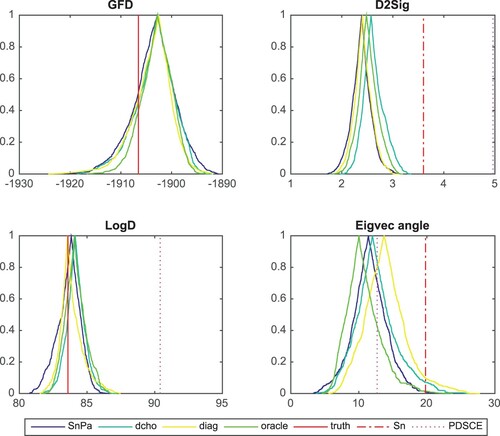
The fiducial estimators have confidence curves peak around the truth in Panels GFD and LogD. In the right two panels, the (majority of) fiducial estimators lie on the left of the dotted-dashed lines, indicating that the estimators are closer to the truth than the sample covariance. The PDSCE estimator falls on the right edge of the Panel D2Sig shows that it is not as close to the truth. As before, the PDSCE estimator overestimates the covariance determinant. Here, burn in = 5000, window = 10,000.

3.5. Model selection for the general case

Often time in practice, to obtain enough statistical power or simply for feasibility, sparse covariates/covariances assumptions are imposed. The exact sparse structure is usually unknown, model selection is required to determine the appropriate parameter space.

Since GFD behaves like the likelihood function, in order to avoid over-fitting, a penalty term on the parameter space needs to be included in the model selection process (Hannig et al., 2016).

For the general case, we propose the following penalty function that is based on the Minimum Description Length (MDL) Rissanen (1978) for a model $\mathcal{M}$: (19) $\begin{array}{r}{q}_{\mathcal{M}}\left(n\right)=\exp \left\{-\sum _{i=1}^p\left[\frac{1}{2}{p}_i\log \left(np\right)+\log \left(\begin{array}{c}p\\ p_i\end{array}\right)\right]\right\},\end{array}$(19) where $\mathcal{M}$ corresponds to a $p\times p$ matrix with $p_i$ many non-fixed-zero elements in its ith row, and n is the number of observations.

The penalised GFD of A is therefore (20) $\begin{array}{rl}& r_p(A|\mathcal{M},\mathit{y})\propto r(A|\mathcal{M},\mathit{y})\\ & \times \exp \left\{-\sum _{i=1}^p\left[\frac{1}{2}{p}_i\log \left(np\right)+\log \left(\begin{array}{c}p\\ p_i\end{array}\right)\right]\right\}.\end{array}$(20)

3.6. Sampling in the general case with sparse locations unknown

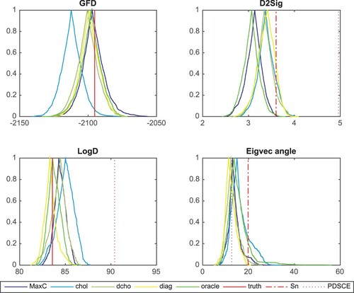
In the general case with sparse locations unknown, we further assume that there is a maximum number of nonzeros per column allowed, denoted as maxC. This additional constraint can be viewed as each predictor only contribute to few tuples of the multivariate response. This assumption has been implemented to reduce the search space for RJMCMC. The starting states include MaxC ($S_n^{0.5}$, restricted to maxC, in blue) along with chol (in cyan), dcho (in artichoke), diag (in yellow) and true (in green) as before. We will revisit the example discussed in Section 3.4.

(See Figure 2). In the left two panels, the fiducial estimators peak at the true fiducial likelihood and covariance determinant. The distance comparison plot (top right) show that the estimators are closer to the truth than both the sample covariance matrix and the PDSCE estimator. Bottom right panel shows that the leading eigenvector of the estimators are as close to the truth as for sample covariance and the PDSCE estimator as in Figure 1. Here, burn in = 50,000, window = 10,000.

Figure 2. Similar to Figure 1, the fiducial estimators are better than both the sample covariance matrix and the PDSCE estimator in this case.

Additional simulations are included in the supplementary document.

4. Clique model

4.1. Jacobian for the clique model

Assume that the coordinates of $\mathit{y}$ are broken into cliques, i.e., coordinates i and j are correlated if i, j belong to the same clique and independent otherwise. By simply swapping rows and columns of the covariate matrix, we can arrive at a block diagonal form. Without loss of generality, suppose that A is a block diagonal matrix with block sizes $g_1,\dots ,g_k$. Then its model $\mathcal{M}$ defines the parameter space ${\otimes }_{i=1}^k{\mathbb{R}}^{g_i\times g_i}$. Given $\mathcal{M}$, as an extension of the full model, the GFD function in this case becomes a composite of inverse Wishart distributions: (21) $\begin{array}{rl}r(\mathrm{\Sigma }|\mathit{y},\mathcal{M})& =\prod _{i=1}^k\frac{|n{S}_n^i{|}^{\frac{n}{2}}}{2^{\frac{n{g}_i}{2}}{\mathrm{\Gamma }}_{g_i}\left({\displaystyle \frac{n}{2}}\right)}|{\mathrm{\Sigma }}^i{|}^{-\frac{n+g_i+1}{2}}\\ & \times \exp \left\{-\frac{1}{2}\text{tr}\left(n{S}_n^i({\mathrm{\Sigma }}^i{)}^{-1}\right)\right\},\end{array}$(21) where $S_n^i$ and ${\mathrm{\Sigma }}^i$ are the sample covariance and covariance component of the ith clique, and ${\mathrm{\Gamma }}_{g_i}(\cdot )$ is the $g_i$ dimensional multivariate gamma function.

4.2. Theoretic results for the clique models

Recall that under the full model, $\begin{array}{rl}& r\left(A|\mathit{y}\right)\propto {\left|\text{det}\left(S_n\right)\right|}^{\frac{p}{2}}\left(2\text{π}{)}^{-\frac{np}{2}}|\text{det}\right(A){|}^{-(n+p)}\\ & \times \exp \left[-\frac{1}{2}\text{tr}\left\{n{S}_n\right(A{A}^{\mathrm{T}}{)}^{-1}\}\right].\end{array}$For clique model selection, we need to evaluate the normalising constant. (22) $\begin{array}{r}\int J(\mathit{y},A)f\left(\mathit{y}|A\right)\mathrm{d}A=\frac{{\text{π}}^{(p^2-np)/2}{\left|\text{det}\left(S_n\right)\right|}^{\frac{p}{2}}{\mathrm{\Gamma }}_p\left({\displaystyle \frac{n}{2}}\right)}{|\text{det}\left(n{S}_n\right){|}^{n/2}{\mathrm{\Gamma }}_p\left({\displaystyle \frac{p}{2}}\right)}.\end{array}$(22) The detailed derivation is provided in Appendix A.3.

Let us denote by $\mathcal{M}$ a clique model; a collection of k cliques – sets of indexes that are related to each other. The coordinates are assumed independent if they are not in the same cliques. For any positive-definite symmetric matrix S, whose dimension is compatible with $\mathcal{M}$, we denote $S^{\mathcal{M}}$ as the matrix obtained from S by setting the off-diagonal entries that corresponds to pairs of indexes not in the same clique within $\mathcal{M}$ to zero. Note that $S^{\mathcal{M}}$ is a block diagonal (after possible permutations of rows and columns) positive-definite symmetric matrix.

The classical Fischer–Hadamard inequality (Fischer, 1908) implies that for any positive definite symmetric matrix S and any clique model $\text{det}\left(S\right)\le \text{det}\left(S^{\mathcal{M}}\right).$ Ipsen Lee (2011) provides a useful lower bound. Let ρ be the spectral radius and λ be the smallest eigenvalue of $\left(S^{\mathcal{M}}{)}^{-1}\right(S-S^{\mathcal{M}})$, (23) $\begin{array}{r}{\text{e}}^{-\frac{p{\rho }^2}{1+\lambda }}\text{det}\left(S^{\mathcal{M}}\right)\le \text{det}\left(S\right)\le \text{det}\left(S^{\mathcal{M}}\right).\end{array}$(23) Assume the clique sizes are $g_1,\dots ,g_k.$ Then the GFD of the model is (24) $\begin{array}{r}r\left(\mathcal{M}|\mathit{y}\right)\propto \frac{{\pi }^{\frac{\sum _{i=1}^k{g}_i^2}{2}}}{|\text{det}{S}_n^{\mathcal{M}}{|}^{\frac{n}{2}}}\prod _{i=1}^k{C}_{\mathcal{M},i}\left(\mathit{y}\right)\frac{{\mathrm{\Gamma }}_{g_i}\left({\displaystyle \frac{n}{2}}\right)}{{\mathrm{\Gamma }}_{g_i}\left({\displaystyle \frac{g_i}{2}}\right)},\end{array}$(24) where $C_{\mathcal{M},i}\left(\mathit{y}\right)$ denotes the Jacobian constant term $|\text{det}\left(S_{n,i}\right){|}^{\frac{g_i}{2}}$ computed only using the observations in the ith clique.

In the remaining part of this section, we consider the dimension of $\mathit{y}$ as a fixed number p and the sample size $n\to \mathrm{\infty }$. Similar arguments could be extended to $p\to \mathrm{\infty }$ with $p/\sqrt{n}\to 0$.

Given two clique models ${\mathcal{M}}_1$ and ${\mathcal{M}}_2$. We write ${\mathcal{M}}_1\subset {\mathcal{M}}_2$ if cliques in ${\mathcal{M}}_2$ are obtained by merging cliques in ${\mathcal{M}}_1$. Consequently, ${\mathcal{M}}_2$ has fewer cliques and these cliques are larger than ${\mathcal{M}}_1$. Let ${\mathcal{M}}_0,{\mathrm{\Sigma }}_0$ be the ‘true’ clique model and covariance matrix used to generate the observed data. We will call all the clique models $\mathcal{M}$ satisfying ${\mathrm{\Sigma }}_0^{\mathcal{M}}={\mathrm{\Sigma }}_0$ compatible with the true covariance matrix. We assume that ${\mathcal{M}}_0\subset \mathcal{M}$ for all clique models compatible with ${\mathrm{\Sigma }}_0$.

The following theorem provides some guidelines for choosing penalty function $q_{\mathcal{M}}\left(n\right)$. Its proof is included in the appendix. Define the penalised GFD of the model as $r_p\left(\mathcal{M}|\mathit{y}\right)=r\left(\mathcal{M}|\mathit{y}\right)q_{\mathcal{M}}\left(n\right)$.

Theorem 4.1

For any clique model $\mathcal{M}$ that is not compatible with ${\mathrm{\Sigma }}_0$, assume $\mathrm{d}\mathrm{e}\mathrm{t}\left({\mathrm{\Sigma }}_0\right)<\mathrm{d}\mathrm{e}\mathrm{t}\left({\mathrm{\Sigma }}_0^{\mathcal{M}}\right)$ and the penalty ${\mathrm{e}}^{-an}{q}_{\mathcal{M}}\left(n\right)/q_{{\mathcal{M}}_0}\left(n\right)\to 0$ for all a>0 as $n\to \mathrm{\infty }$.

For any clique model $\mathcal{M}$ compatible with ${\mathrm{\Sigma }}_0$ assume that $q_{\mathcal{M}}\left(n\right)/q_{{\mathcal{M}}_0}\left(n\right)$ is bounded.

Then as $n\to \mathrm{\infty }$ with p held fixed $r_p\left({\mathcal{M}}_0|\mathit{Y}\right)\stackrel{P}{⟶}1.$

The exact form of the penalty function depends on the norm choice for the Jacobian. Under the ${\ell }_2$-norm, the following penalty function works well. (25) $\begin{array}{r}{q}_{\mathcal{M}}\left(n\right)=\exp \left\{-\sum _{i=1}^k\left[\frac{1}{4}{g}_i^2\log \left(n\right)-\frac{1}{2}{g}_i^2\log \left(g_i\right)\right]\right\}.\end{array}$(25) It is easy to check that Equation (25(25) $\begin{array}{r}{q}_{\mathcal{M}}\left(n\right)=\exp \left\{-\sum _{i=1}^k\left[\frac{1}{4}{g}_i^2\log \left(n\right)-\frac{1}{2}{g}_i^2\log \left(g_i\right)\right]\right\}.\end{array}$(25) ) satisfies Theorem 4.1.

4.3. Sampling from a clique model

The estimation of cliques is closely related to applications in network analysis, such as communities of people in social networks and gene regulatory network. Recall the penalised clique model GFD introduced in Section 4.2, $r_p\left(\mathcal{M}|\mathit{y}\right)\propto \frac{{\text{π}}^{\frac{\sum _{i=1}^k{g}_i^2}{2}}}{|\text{det}{S}_n^{\mathcal{M}}{|}^{\frac{n}{2}}}\prod _{i=1}^k{C}_{\mathcal{M},i}\left(\mathit{y}\right)\frac{{\mathrm{\Gamma }}_{g_i}\left({\displaystyle \frac{n}{2}}\right)}{{\mathrm{\Gamma }}_{g_i}\left({\displaystyle \frac{g_i}{2}}\right)}{q}_{\mathcal{M}}\left(n\right).$Assuming that both the number of cliques k and the clique sizes $g_k$'s are unknown, the clique structure can be estimated via Gibbs sampler. The first example shows the simulation result for a $200\times 200$ covariance matrix (Figure 3). We consider the covariance matrix to be with 1's on the diagonal and $(i,j)$th entry being 0.5 if the coordinate $(i,j)$ belongs to a clique. 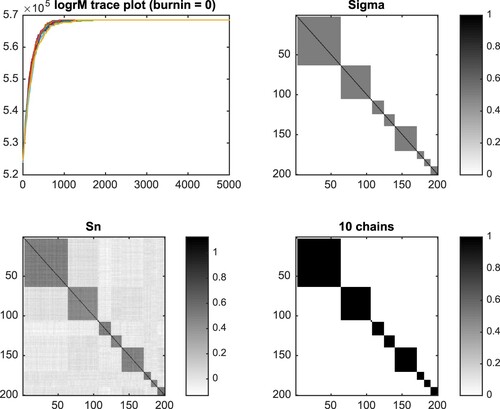From top down, left to right, Figure 3 shows the trace plot for $\log \left(r_p\right(\mathcal{M}|\mathit{y}\left)\right)$ without normalising constant, true covariance Σ, sample covariance $S_n$, and the fiducial probability of the estimated cliques based on the 10 Gibbs sampler Markov chains with random initial states. The trace plot helps to monitor the convergence. The fiducial probability of cliques panel reveals the clique structure precisely. The last panel is the aggregate result of 4000 iterations with burn in = 1000 from the 10 Markov chains.

Figure 3. Result for k = 10, p = 200, n = 1000. The trace plot (top left) shows that the chains converge quickly. Although $\frac{n}{p}$ is small, the sample covariance (bottom left) roughly captures the shape of true covariance (top right). The last panel (bottom right) shows that the fiducial estimate captures the true clique structure perfectly.

The covariance estimators can be obtained by sampling from inverse Wishart distributions based on the estimated clique structure. Figure 4 shows the confidence curves of four statistics for estimated covariance matrix $\hat{\mathrm{\Sigma }}$: log-transformed generalised fiducial likelihood (SlogGFD), distance to Σ (D2Sig), log-determinant (LogD), and angle between the leading eigenvectors of $\hat{\mathrm{\Sigma }}$ and Σ (Eigvec angle). The truth for SlogGFD and LogD is shown as red solid vertical lines. In D2Sig and Eigvec angle panels, we include comparisons to sample covariance as red dotted-dashed vertical lines. In addition, we compute the point estimation via the Positive Definite Sparse Covariance Estimators (PDSCE) method introduced in Rothman (2012). Its corresponding statistics are shown as magenta dotted vertical lines. In this example, the fiducial estimates peak near the truth in Panels SlogGFD and LogD. The estimated covariance matrices all appear to be more similar to Σ than $S_n$ as shown in panels D2Sig and Eigvec angle. The PDSCE estimator is even closer to Σ in terms of FM-distance; it however greatly overestimates $\text{det}\mathrm{\Sigma }$.

Figure 4. Confidence curve plots for estimated covariance matrix. k=10,p=200,n= 1000. Comparing to the sample covariance, the estimators are closer to Σ. The PDSCE estimator shows even smaller FM-distance to Σ, it, however, greatly overestimates $\text{det}\mathrm{\Sigma }$.

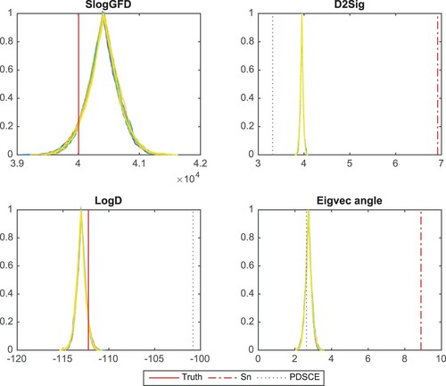
The PDSCE method produces a good point estimator to the covariance matrix. It is worth noting that our method shows similar performance with the benefit of producing a distribution of estimators.

With the same underlying clique model, we generate 200 data sets. Then we apply our method with a random Markov chain starting point and compute the one-sided p-values for the estimate covariance log determinant. With the same true covariance matrix, a new set of 1000 observations are generated for each simulation. Figure 5 shows the quantile–quantile plot of the p-values against the uniform [0,1] distribution. The dotted-dashed envelope is the 95% coverage band. It shows a well-calibrated 95% confidence interval. The p-value curve (in green) is well enclosed by the envelope, indicating good calibration of the coverage.

Figure 5. 95% coverage plots for 200 repeated simulations. k=10,p=200,n= 1000. The p-values (in green) roughly follow a uniform [0,1] distribution, and they lie inside of the envelope.

5. Discussion

Covariance estimation is an important problem in statistics. In this manuscript, we propose to look into this classical problem via a generalised fiducial approach. We demonstrate that, under mild assumptions, the GFD of the covariate matrix is asymptotically normal. In addition, we discuss the clique model and show that the fiducial approach is a powerful tool for identifying clique structures, even when the dimension of the parameter space is large and the ratio n/p is small. To identify the covariance structure for non-clique models, in contrast to typical sparse covariance/precision matrix assumptions, we look at cases where the ratio n/p is small and the covariate matrix is sparse. This ‘unusual’ sparsity assumption arises in applications where multiple dependent variables contribute to several response variables collaboratively. The fiducial approach allows us to obtain a distribution of covariance estimators that are better than sample covariance and comparable to the PDSCE estimator. The distances to true covariance matrix show that as dimension increases, the fiducial estimators become closer to the true covariance matrix.

Similar to Bayesian approaches, generalised fiducial inference produces a distribution of estimators, yet the two methods differ fundamentally. Bayesian methods rely on prior distributions on the parameter of interest, while fiducial approaches depend on the data generating equation. In the framework discussed here, the data generating mechanism is natural to establish than choosing appropriate priors while some other times priors are easier to construct.

Estimating sparse covariance matrix without knowing the fixed zeros is a hard problem. While our approach shows promising results for the clique model, for the general case it still suffers from a few drawbacks: (1) due to the nature of RJMCMC, the computational burden can be significant if the matrix is not very sparse; (2) to limit the search space, a row/column-wise sparsity upper bound needs to be chosen based on prior knowledge of the data type; (3) the results presented in this manuscript assume a squared covariate matrix, which can be limited to direct applications to high-throughput data. Furthermore, a more sophisticated way of choosing initial states and mixing method can improve the efficiency of our algorithm. It is possible and well worth it to extend our current work to more general cases.

Disclosure statement

No potential conflict of interest was reported by the author(s).

Additional information

Funding

Shi's research was supported in part by the National Library of Medicine Institutional Training Grant T15 LM009451. Hannig's research was supported in part by the National Science Foundation (NSF) under Grant Nos. 1512945, 1633074, and 1916115. Lee's research was supported in part by the NSF under Grant No. 1512945 and 1513484.

Notes on contributors

W. Jenny Shi

W. Jenny Shi obtained her PhD in Statistics from the University of North Carolina. From 2015 to 2018, she was a National Institute of Health postdoctoral fellow at the University of Colorado. She is now a Quantitative Strategist at MassMutual, specializing in financial modeling and strategic initiatives.

Jan Hannig

Jan Hannig received his Mgr (MS equivalent) in mathematics in 1996 from the Charles University, Prague, Czech Republic. He received Ph.D. in statistics and probability in 2000 from Michigan State University under the direction of Professor A.V. Skorokhod. From 2000 to 2008 he was on the faculty of the Department of Statistics at Colorado State University where he was promoted to an Associate Professor. He has joined the Department of Statistics and Operation Research at the University of North Carolina at Chapel Hill in 2008 and was promoted to Professor in 2013. He is an elected member of International Statistical Institute and a fellow of the American Statistical Association and Institute of Mathematical Statistics.

Randy C. S. Lai

Randy C. S. Lai obtained his Ph.D. in Statistics from the University of California, Davis (UC Davis). In 2015–2019 he was an Assistant Professor at the University of Maine. He is now a Visiting Assistant Professor at UC Davis, and he will join Google as a Data Scientist in Spring 2021. His research interests include fiducial inference and statistical computing.

Thomas C. M. Lee

Thomas C. M. Lee is Professor of Statistics and Associate Dean for the Faculty in Mathematical and Physical Sciences at the University of California, Davis. He is an elected Fellow of the American Association for the Advancement of Science (AAAS), the American Statistical Association (ASA), and the Institute of Mathematical Statistics (IMS). From 2013 to 2015 he served as the editor-in-chief for the Journal of Computational and Graphical Statistics, and from 2015 to 2018 he served as the Chair of the Department of Statistics at UC Davis. His recent research interests include astrostatistics, fiducial inference, machine learning, and statistical image and signal processing.

Appendix

A.1. Regularity conditions and Jacobian formula

Before proving the theorem on consistency of the GFD, we will first define the δ-neighbourhood of $A_0$ and establish some regularity conditions on the likelihood function and Jacobian formula (Propositions A.1, A.2, 3.1).

Definition A.1

For a fixed covariate matrix $A_0$ and $\delta \ge 0$, define the δ-neighbourhood of $A_0$ as the set $B(A_0,\delta )=\{A:\mathbf{d}(A{A}^{\mathrm{T}},A_0{A}_0^{\mathrm{T}})\le \delta \}$. Recall that $\mathbf{d}$ is the FM-distance (17(17) $\begin{array}{r}\mathbf{d}(M,N)=\sqrt{\sum _{i=1}^n{\log }^2{\lambda }_i(M,N)}.\end{array}$(17) ).

Proposition A.1

For any $\delta >0$ there exists $ϵ>0$ such that $P_{A_0}\left\{\underset{A\notin B(A_0,\delta )}{sup}\frac{1}{n}\left(L_n\right(A)-L_n(A_0\left)\right)\le -ϵ\right\}\to 1,$where $L_n\left(A\right)=\log f(\mathit{y},A)=\sum _{i=1}^n\log f(y_i,A).$

Proof.

Let $\mathrm{\Sigma }=A{A}^{\mathrm{T}},{\mathrm{\Sigma }}_0=A_0{A}_0^{\mathrm{T}}$. Denote $S_n$ as the sample covariance matrix as before, $n\in \mathbb{N}$. Since $S_n$ is the maximum likelihood estimator, we have $\begin{array}{rl}& S_n⟹P_{A_0}{\mathrm{\Sigma }}_0,\mathrm{i}.\mathrm{e}.,\\ & \mathrm{\forall }r>0,P_{A_0}\left(\right\{\omega :\mathbf{d}\left(S_n\right(\omega ),{\mathrm{\Sigma }}_0)\ge r\left\}\right)\to 0.\end{array}$Define $L_{\delta ,n}=\{\omega :\mathbf{d}(S_n\left(\omega \right),{\mathrm{\Sigma }}_0)<\delta /2\}$. For an arbitrary $\omega \in L_{\delta ,n},$ assume that ${\lambda }_i^{†}$'s and ${\lambda }_i^{\ast }$'s are the eigenvalues of $S_n\left(\omega \right){\mathrm{\Sigma }}^{-1}$ and $S_n\left(\omega \right){\mathrm{\Sigma }}_0^{-1}$, respectively. Suppose that $A\notin B(A_0,\delta )$, then $\begin{array}{rl}\delta <\mathbf{d}(\mathrm{\Sigma },{\mathrm{\Sigma }}_0)& \le \mathbf{d}(\mathrm{\Sigma },S_n(\omega \left)\right)+\mathbf{d}\left(S_n\right(\omega ),{\mathrm{\Sigma }}_0)\\ & <\mathbf{d}(\mathrm{\Sigma },S_n(\omega \left)\right)+\delta /2\\ & \Rightarrow \mathbf{d}(\mathrm{\Sigma },S_n(\omega \left)\right)=\sqrt{\sum _{i=1}^p{\log }^2{\lambda }_i^{†}}>\delta /2.\end{array}$So there exists $k\in \{1,2,\dots ,p\}$, such that ${\ln }^2{\lambda }_k^{†}>\frac{{\delta }^2}{4p}$, then $\begin{array}{rl}& \ln {\lambda }_k-{\lambda }_k<max\left\{\frac{\delta }{2\sqrt{p}}-\exp \left(\frac{\delta }{2\sqrt{p}}\right),\right.\\ & -\left.\frac{\delta }{2\sqrt{p}}-\exp \left(-\frac{\delta }{2\sqrt{p}}\right)\right\}:=m_{\delta }\end{array}$due to the fact that the function $g\left(\lambda \right)=\ln \lambda -\lambda$ is concave with unique maxima $\lambda =1$; $g\left(1\right)=-1$.

Meanwhile, $\begin{array}{rl}& \frac{1}{n}\left(L_n\right(A)-L_n(A_0\left)\right)\left(\omega \right)\\ & =-\ln |\text{det}\left(A\right)|-\frac{1}{2}\text{tr}\left\{S_n\right(\omega \left){\mathrm{\Sigma }}^{-1}\right\}\\ & +\ln |\text{det}\left(A_0\right)|+\frac{1}{2}\text{tr}\left\{S_n\right(\omega \left){\mathrm{\Sigma }}_0^{-1}\right\}\\ & =\frac{1}{2}\ln \left(S_n\right(\omega \left){\mathrm{\Sigma }}^{-1}\right)-\frac{1}{2}\text{tr}\left\{S_n\right(\omega \left){\mathrm{\Sigma }}^{-1}\right\}\\ & -\frac{1}{2}\ln \left(S_n\right(\omega \left){\mathrm{\Sigma }}_0^{-1}\right)+\frac{1}{2}\text{tr}\left\{S_n\right(\omega \left){\mathrm{\Sigma }}_0^{-1}\right\}\\ & =\frac{1}{2}\left\{\sum _{i=1}^p(\ln {\lambda }_i^{†}-{\lambda }_i^{†})-\sum _{i=1}^p(\ln {\lambda }_i^{\ast }-{\lambda }_i^{\ast })\right\}\\ & <\frac{1}{2}\left\{-(p-1)+m_{\delta }+p\right\}\\ & =\frac{1}{2}(m_{\delta }+1).\end{array}$This implies $\underset{A\notin B(A_0,\delta )}{sup}\frac{1}{n}\left(L_n\right(A)-L_n(A_0\left)\right)\left(\omega \right)\le \frac{1}{2}(m_{\delta }+1)<0.$Let $ϵ=-\frac{1}{2}(m_{\delta }+1),U_{\delta ,n}=\{\omega :\underset{A\notin B(A_0,\delta )}{sup}\frac{1}{n}(L_n\left(A\right)-L_n\left(A_0\right)\left)\right(\omega )\le -ϵ\}$. Then $L_{\delta ,n}\subseteq U_{\delta ,n}$. Notice that $\begin{array}{rl}1& =\underset{n\to \mathrm{\infty }}{lim}{P}_{A_0}\left(L_{\delta ,n}\right)=\underset{n\to \mathrm{\infty }}{lim inf}{P}_{A_0}\left(L_{\delta ,n}\right)\\ & \le \underset{n\to \mathrm{\infty }}{lim inf}{P}_{A_0}\left(U_{\delta ,n}\right)\le \underset{n\to \mathrm{\infty }}{lim sup}{P}_{A_0}\left(U_{\delta ,n}\right)\le 1.\end{array}$Therefore, $\underset{n\to \mathrm{\infty }}{lim}{P}_{A_0}\left(U_{\delta ,n}\right)=1.$

Proposition A.2

Let $L_n(\cdot )$ be as above. Then for any $\delta >0$ $\underset{A\notin B(A_0,\delta )}{inf}\frac{\underset{\begin{array}{c}\mathbf{i}=\{i_1,\dots ,i_p\}\\ 1\le i_1<\cdots <i_p\le n\end{array}}{min}\log f(A,{\mathit{y}}_{\mathbf{i}})}{|L_n\left(A\right)-L_n\left(A_0\right)|}⟹A_{0}0,$where $f(A,{\mathit{y}}_{\mathbf{i}})$ is the joint likelihood of p observations $y_{i_1},\dots ,y_{i_p}$.

Proof.

Note that $\begin{array}{rl}& \underset{A\notin B(A_0,\delta )}{inf}\frac{\underset{\begin{array}{c}\mathbf{i}=\{i_1,\dots ,i_p\}\\ 1\le i_1<\cdots <i_p\le n\end{array}}{min}\log f(A,{\mathit{y}}_{\mathbf{i}})}{|L_n\left(A\right)-L_n\left(A_0\right)|}\\ & \le \frac{\underset{A\notin B(A_0,\delta )}{inf}\underset{\begin{array}{c}\mathbf{i}=\{i_1,\dots ,i_p\}\\ 1\le i_1<\cdots <i_p\le n\end{array}}{min}\log f(A,{\mathit{y}}_{\mathbf{i}})}{\underset{A\notin B(A_0,\delta )}{inf}|L_n\left(A\right)-L_n\left(A_0\right)|}.\end{array}$For any $A\notin B(A_0,\delta )$, denote $\mathrm{\Sigma }=A{A}^{\mathrm{T}},{\mathrm{\Sigma }}_0=A_0{A}_0^{\mathrm{T}}$ and let t>0, we have $\begin{array}{rl}& P_{A_0}\left(\underset{\begin{array}{c}\mathbf{i}=\{i_1,\dots ,i_p\}\\ 1\le i_1<\cdots <i_p\le n\end{array}}{min}\log f(A,{\mathit{y}}_{\mathbf{i}})\le -t\log n\right)\\ & \le P_{A_0}\left(\underset{i=1,\dots ,n}{min}\log f(A,Y_i)\le -\frac{t\log n}{p}\right)\\ & =1-{\left[1-P_{A_0}\left(-\log f(A,Y_i)\ge -\frac{t\log n}{p}\right)\right]}^n\\ & \le 1-{\left[1-\frac{p{\text{E}}_{A_0}(-\log f(A,Y_i\left)\right)}{t\log n}\right]}^n\left(\mathrm{M}\mathrm{a}\mathrm{r}\mathrm{k}\mathrm{o}\mathrm{v}\mathrm{i}\mathrm{n}\mathrm{e}\mathrm{q}\mathrm{u}\mathrm{a}\mathrm{l}\mathrm{i}\mathrm{t}\mathrm{y}\right)\\ & =1-{\left[1-\frac{p(\log (2\pi )+\log \text{det}(\mathrm{\Sigma })+\text{tr}\{{\mathrm{\Sigma }}^{-1}{\mathrm{\Sigma }}_0\left\}\right)}{2t\log n}\right]}^n\\ & \to 0,\mathrm{a}\mathrm{s}n\to \mathrm{\infty }.\end{array}$Note that the numerator goes to $-\mathrm{\infty }$ at most as fast as $-t\log n$. Meanwhile, for a fixed n and any $\omega \in L_{\delta ,n}=\{\omega :\mathbf{d}(S_n\left(\omega \right),{\mathrm{\Sigma }}_0)<\delta /2\}$, $\begin{array}{rl}& \underset{A\notin B(A_0,\delta )}{inf}|L_n\left(A\right)-L_n\left(A_0\right)|\\ & =-\underset{A\notin B(A_0,\delta )}{sup}{L}_n\left(A\right)-L_n\left(A_0\right)\ge ϵn.\end{array}$By Proposition (A.1), $\underset{n\to \mathrm{\infty }}{lim}{P}_{A_0}\left(\underset{A\notin B(A_0,\delta )}{inf}|L_n\left(A\right)-L_n\left(A_0\right)|\ge ϵn\right)=1,$i.e., the denominator goes to infinity at least as fast as $ϵn$.

Proof of Proposition 3.1.

Proof of Proposition 3.1

Given an ordered index vector $\mathbf{r}=(r_1,\dots ,r_l)$, let $E_{\mathbf{r}}=(e_{r_1};\cdots ;e_{r_l})$, where each $e_{r_j}$ is a $1\times p$ vector with 1 in the $r_j$th tuple and 0 everywhere else. Denote $-\mathbf{r}=\{1,\dots ,p\}\setminus \mathbf{r}$.

Under the ${\ell }_2$-norm, $\begin{array}{rl}J(\mathit{y},A)& =\sqrt{\prod _{i=1}^p\text{det}\left(U_i^{\mathrm{T}}{U}_i/n\right)}\\ & =\sqrt{\prod _{i=1}^p\text{det}\left(E_{-S_i}^{\mathrm{T}}{A}^{-1}{S}_n(A^{-1}{)}^{\mathrm{T}}{E}_{-S_i}\right)},\end{array}$where $S_i$ is the list of indexes of fixed zeros in the ith row of A.

By the Strong Law of Large Numbers for $S_n$ and continuity of $J(\mathit{y},A)$, $\begin{array}{rl}& J(\mathit{y},A)⟶\sqrt{\prod _{i=1}^p\text{det}\left(E_{-S_i}^{\mathrm{T}}{A}^{-1}{\mathrm{\Sigma }}_0(A^{-1}{)}^{\mathrm{T}}{E}_{-S_i}\right)}\\ & :={\pi }_{{\mathrm{\Sigma }}_0}\left(A\right)\mathrm{a}.\mathrm{s}.\end{array}$Note that both $P_n=J(\mathit{y},A)$ and $P_0={\pi }_{{\mathrm{\Sigma }}_0}\left(A\right)$ are polynomials of entries of $A^{-1}.$ If the domain of A is in compact, the coefficients of $P_n$ converge to the coefficients of $P_0$ uniformly. Furthermore, the derivative is bounded, hence $P_n$ is equicontinuous. We have $J(\mathit{y},A)⟹\mathrm{a}.\mathrm{s}.{\pi }_{{\mathrm{\Sigma }}_0}\left(A\right)$ uniformly on compacts in A.

A.2. Proof of Theorem 3.1

Proof.

Proposition 3.1 implies $\underset{A\in B(A_0,\delta )}{sup}|J(\mathit{y},A)-{\pi }_{{\mathrm{\Sigma }}_0}\left(A\right)|\to 0\mathrm{a}.\mathrm{s}.P_{A_0}.$ $\begin{array}{rl}{\pi }^{\ast }(B,\mathit{y})& =\frac{J\left(\mathit{y},{\hat{A}}_n+{\displaystyle \frac{B}{\sqrt{n}}}\right)f\left(\mathit{y}|{\hat{A}}_n+{\displaystyle \frac{B}{\sqrt{n}}}\right)}{{\displaystyle {\int }_{{\mathbb{R}}^{p^2}}J\left(\mathit{y},{\hat{A}}_n+\frac{C}{\sqrt{n}}\right)f\left(\mathit{y}|{\hat{A}}_n+\frac{C}{\sqrt{n}}\right)\mathrm{d}C}}\\ & =\frac{\begin{array}{c}J\left(\mathit{y},{\hat{A}}_n+{\displaystyle \frac{B}{\sqrt{n}}}\right)\\ \exp \left[L_n\left({\hat{A}}_n+{\displaystyle \frac{B}{\sqrt{n}}}\right)-L_n\left(\widehat{A_n}\right)\right]\end{array}}{\begin{array}{c}{\displaystyle {\int }_{{\mathbb{R}}^{p^2}}J\left(\mathit{y},{\hat{A}}_n+\frac{C}{\sqrt{n}}\right)}\\ \times \exp \left[L_n\left({\hat{A}}_n+{\displaystyle \frac{C}{\sqrt{n}}}\right)-L_n\left(\widehat{A_n}\right)\right]\mathrm{d}C.\end{array}}\end{array}$Notice that $H=-\frac{1}{n}\frac{{\mathrm{\partial }}^2}{\mathrm{\partial }A\mathrm{\partial }A}\left(\widehat{A_n}\right)\to I\left(A_0\right)\mathrm{a}.\mathrm{s}.P_{A_0}.$It suffices to show that (A1) $\begin{array}{r}\begin{array}{rl}& {\int }_{{\mathbb{R}}^{p^2}}\left|J\left(\mathit{y},{\hat{A}}_n+\frac{C}{\sqrt{n}}\right)\exp \left[L_n\left({\hat{A}}_n+\frac{C}{\sqrt{n}}\right)-L_n\left(\widehat{A_n}\right)\right]\right.\\ & \left.-{\pi }_{{\mathrm{\Sigma }}_0}\left(A_0\right)\exp \left[\frac{-C^{T}I\left(A_0\right)C}{2}\right]\right|\mathrm{d}C⟹P_{A_0}0.\end{array}\end{array}$(A1) Let $C_x$ be the ijth entry of C, where $x=i+(p-1)j$. By Taylor Theorem, $\begin{array}{rl}{L}_n\left({\hat{A}}_n+\frac{C}{\sqrt{n}}\right)& =L_n\left({\hat{A}}_n\right)+\sum _{x=1}^{p^2}\left(\frac{C_x}{\sqrt{\left(n\right)}}\right)\frac{\mathrm{\partial }}{\mathrm{\partial }{A}_x}{L}_n\left({\hat{A}}_n\right)\\ & +\frac{1}{2}\sum _{x=1}^{p^2}\sum _{y=1}^{p^2}\left(\frac{C_x{C}_y}{(\sqrt{\left(n\right)}{)}^2}\right)\\ & \times \frac{{\mathrm{\partial }}^2}{\mathrm{\partial }{A}_x\mathrm{\partial }{A}_y}{L}_n\left({\hat{A}}_n\right)\\ & +\frac{1}{6}\sum _{x=1}^{p^2}\sum _{y=1}^{p^2}\sum _{z=1}^{p^2}\left(\frac{C_x{C}_y{C}_z}{(\sqrt{\left(n\right)}{)}^3}\right)\\ & \times \frac{{\mathrm{\partial }}^3}{\mathrm{\partial }{A}_x\mathrm{\partial }{A}_y\mathrm{\partial }{A}_z}{L}_n\left(A^{\prime }\right)\\ & =L_n\left({\hat{A}}_n\right)-\frac{C^{\mathrm{T}}HC}{2}+R_n\end{array}$for some $A^{\prime }\in [{\hat{A}}_n,{\hat{A}}_n+\frac{C}{\sqrt{n}}]$. Notice that $R_n=\mathcal{O}p(n^{-3/2}\times ||C||)$. Given any $0<\delta <{\delta }_0$ and t>0, the parameter space ${\mathbb{R}}^{p^2}$ can be partitioned into three regions: $\begin{array}{rl}{S}_1& =\{C:||C||<t\log \sqrt{n}\};\\ S_2& =\{C:t\log \sqrt{n}<||C||<\delta \sqrt{n}\};\\ S_3& =\{C:||C||>\delta \sqrt{n}\}.\end{array}$On $S_1\cup S_2$, $\begin{array}{rl}& {\int }_{S_1\cup S_2}\left|J\left(\mathit{y},{\hat{A}}_n+\frac{C}{\sqrt{n}}\right)\exp \left[L_n\left({\hat{A}}_n+\frac{C}{\sqrt{n}}\right)-L_n\left({\hat{A}}_n\right)\right]\right.\\ & \left.-{\pi }_{{\mathrm{\Sigma }}_0}\left(A_0\right)\exp \left[\frac{-C^{\mathrm{T}}I\left(A_0\right)C}{2}\right]\right|\mathrm{d}C\\ & \le {\int }_{S_1\cup S_2}\left|J\left(\mathit{y},{\hat{A}}_n+\frac{C}{\sqrt{n}}\right)-{\pi }_{{\mathrm{\Sigma }}_0}\left({\hat{A}}_n+\frac{C}{\sqrt{n}}\right)\right|\\ & \times \exp \left[L_n\left({\hat{A}}_n+\frac{C}{\sqrt{n}}\right)-L_n\left({\hat{A}}_n\right)\right]\mathrm{d}C\\ & +{\int }_{S_1\cup S_2}\left|{\pi }_{{\mathrm{\Sigma }}_0}\left({\hat{A}}_n+\frac{C}{\sqrt{n}}\right)\right.\\ & \times \exp \left[L_n\left({\hat{A}}_n+\frac{C}{\sqrt{n}}\right)-L_n\left({\hat{A}}_n\right)\right]\\ & \left.-{\pi }_{{\mathrm{\Sigma }}_0}\left(A_0\right)\exp \left[\frac{-C^{\mathrm{T}}I\left(A_0\right)C}{2}\right]\right|\mathrm{d}C.\end{array}$Since ${\pi }_{{\mathrm{\Sigma }}_0}(\cdot )$ is a proper prior on the region $S_1\cup S_2$, the second term goes to zero by the Bayesian Bernstein–von Mises Theorem (see the proof of Theorem 1.4.2 in Ghosh and Ramamoorthi (2003)).

Next we notice that $\begin{array}{rl}& {\int }_{S_1\cup S_2}\left|J\left(\mathit{y},{\hat{A}}_n+\frac{C}{\sqrt{n}}\right)-{\pi }_{A_0}\left({\hat{A}}_n+\frac{C}{\sqrt{n}}\right)\right|\\ & \times \exp \left[L_n\left({\hat{A}}_n+\frac{C}{\sqrt{n}}\right)-L_n\left({\hat{A}}_n\right)\right]\mathrm{d}C\\ & \le \underset{C\in S_1\cup S_2}{sup}\left|J\left(\mathit{y},{\hat{A}}_n+\frac{C}{\sqrt{n}}\right)-{\pi }_{A_0}\left({\hat{A}}_n+\frac{C}{\sqrt{n}}\right)\right|\\ & \times {\int }_{S_1\cup S_2}\exp \left[L_n\left({\hat{A}}_n+\frac{C}{\sqrt{n}}\right)-L_n\left({\hat{A}}_n\right)\right]\mathrm{d}C.\end{array}$Since $\sqrt{n}({\hat{A}}_n-A_0)⟹\mathcal{D}N(0,I(A_0{)}^{-1})$, we have $P_{A_0}\left[\left\{{\hat{A}}_n+\frac{C}{\sqrt{n}};C\in S_1\cup S_2\right\}\subset B(A_0,{\delta }_0)\right]\to 1.$Furthermore, $L_n\left({\hat{A}}_n+\frac{C}{\sqrt{n}}\right)-L_n\left({\hat{A}}_n\right)=-\frac{C^{\mathrm{T}}HC}{2}+R_n,$so the integral converges in probability to 1. Since $\underset{C\in S_1\cup S_2}{max}\le \delta$ and $J_n\to {\pi }_{{\mathrm{\Sigma }}_0}$, the term goes to 0 in probability.

Turning our attention to $S_3$, notice that $\begin{array}{rl}& {\int }_{S_3}\left|J\left(\mathit{y},{\hat{A}}_n+\frac{C}{\sqrt{n}}\right)\exp \left[L_n\left({\hat{A}}_n+\frac{C}{\sqrt{n}}\right)-L_n\left({\hat{A}}_n\right)\right]\right.\\ & \left.-{\pi }_{{\mathrm{\Sigma }}_0}\left(A_0\right)\exp \left[\frac{-C^{\mathrm{T}}I\left(A_0\right)C}{2}\right]\right|\mathrm{d}C\\ & \le {\int }_{S_3}J\left(\mathit{y},{\hat{A}}_n+\frac{C}{\sqrt{n}}\right)\\ & \times \exp \left[L_n\left({\hat{A}}_n+\frac{C}{\sqrt{n}}\right)-L_n\left({\hat{A}}_n\right)\right]\mathrm{d}C\\ & +{\int }_{S_3}{\pi }_{{\mathrm{\Sigma }}_0}\left(A_0\right)\exp \left[\frac{-C^{\mathrm{T}}I\left(A_0\right)C}{2}\right]\mathrm{d}C.\end{array}$The last integral goes to zero in $P_{A_0}$ because $\underset{S_3}{min}||C||\to \mathrm{\infty }$.

For each $\mathit{y}$, let $\mathbf{i}$ be $\begin{array}{rl}\mathbf{i}& =\underset{\tilde{\mathbf{i}}}{argmin}\left|J\left(\mathit{y},{\hat{A}}_n+\frac{C}{\sqrt{n}}\right)-J\left({\mathit{y}}_{\tilde{\mathbf{i}}},{\hat{A}}_n+\frac{C}{\sqrt{n}}\right)\right|\\ & =\underset{\tilde{\mathbf{i}}}{argmin}h(\mathit{y},C,\tilde{\mathbf{i}}).\end{array}$ $\begin{array}{rl}& {\int }_{S_3}J\left(\mathit{y},{\hat{A}}_n+\frac{C}{\sqrt{n}}\right)\exp \left[L_n\left({\hat{A}}_n+\frac{C}{\sqrt{n}}\right)-L_n\left({\hat{A}}_n\right)\right]\mathrm{d}C\\ & \le {\int }_{S_3}\left\{h(\mathit{y},C,\mathbf{i})f\left({\mathit{y}}_{\mathbf{i}}|{\hat{A}}_n+\frac{C}{\sqrt{n}}\right)\right.\\ & \left.+J\left({\mathit{y}}_{\mathbf{i}},{\hat{A}}_n\frac{C}{\sqrt{n}}\right)f\left({\mathit{y}}_{\mathbf{i}}|{\hat{A}}_n+\frac{C}{\sqrt{n}}\right)\right\}\\ & \times \exp \left[L_n\left({\hat{A}}_n+\frac{C}{\sqrt{n}}\right)\right.\\ & -\left.L_n\left({\hat{A}}_n\right)-\log f\left({\mathit{y}}_{\mathbf{i}}|{\hat{A}}_n+\frac{C}{\sqrt{n}}\right)\right]\mathrm{d}C.\end{array}$Note that as n goes to infinity, the first two product terms, $h(\cdot )f(\cdot )$ and $J(\cdot )f(\cdot )$, are both bounded; the exponent term goes to $-\mathrm{\infty }$ by Proposition A.2, so the integral goes to zero in probability.

Having shown Equation (A1(A1) $\begin{array}{r}\begin{array}{rl}& {\int }_{{\mathbb{R}}^{p^2}}\left|J\left(\mathit{y},{\hat{A}}_n+\frac{C}{\sqrt{n}}\right)\exp \left[L_n\left({\hat{A}}_n+\frac{C}{\sqrt{n}}\right)-L_n\left(\widehat{A_n}\right)\right]\right.\\ & \left.-{\pi }_{{\mathrm{\Sigma }}_0}\left(A_0\right)\exp \left[\frac{-C^{T}I\left(A_0\right)C}{2}\right]\right|\mathrm{d}C⟹P_{A_0}0.\end{array}\end{array}$(A1) ), we now follow Ghosh and Ramamoorthi (2003) and let $\begin{array}{rl}{D}_n& ={\int }_{{\mathbb{R}}^{p^2}}\left|J\left(\mathit{y},{\hat{A}}_n+\frac{C}{\sqrt{n}}\right)\right.\\ & \times \left.\exp \left[L_n\left({\hat{A}}_n+\frac{C}{\sqrt{n}}\right)-L_n\left({\hat{A}}_n\right)\right]\right|\mathrm{d}C.\end{array}$Then the main result to be proven Equation (18(18) $\begin{array}{rl}& {\int }_{{\mathbb{R}}^{p^2}}\left|{\pi }^{\ast }(B,\mathit{y})-\frac{\sqrt{\mathrm{d}\mathrm{e}\mathrm{t}|I\left(A_0\right)|}}{(2\text{π}{)}^p}\right.\\ & \times \left.\exp \{-B^{\mathrm{T}}I(A_0\left)B/2\right\}\right|\mathrm{d}B⟹P_{A_0}0.\end{array}$(18) ) becomes (A2) $\begin{array}{r}\begin{array}{rl}& D_n^{-1}\left\{{\int }_{{\mathbb{R}}^{p^2}}\left|J\left(\mathit{y},{\hat{A}}_n+\frac{B}{\sqrt{n}}\right)\right.\right.\\ & \times \exp \left[L_n\left({\hat{A}}_n+\frac{B}{\sqrt{n}}\right)-L_n\left({\hat{A}}_n\right)\right]\\ & \left.\left.-D_n\frac{\sqrt{\text{det}\left(I\right(A_0\left)\right)}}{(2\text{π}{)}^p}\exp \left(-\frac{B^{\mathrm{T}}I\left(A_0\right)B}{2}\right)\right|\right\}\mathrm{d}B⟹P_{A_0}0.\end{array}\end{array}$(A2) Because $\begin{array}{rl}& {\int }_{{\mathbb{R}}^{p^2}}J(\mathit{y},{\hat{A}}_n)\exp \left(-\frac{B^{\mathrm{T}}I\left(A_0\right)B}{2}\right)\mathrm{d}B\\ & =J(\mathit{y},{\hat{A}}_n){\int }_{{\mathbb{R}}^{p^2}}\exp \left(-\frac{B^{\mathrm{T}}I\left(A_0\right)B}{2}\right)\mathrm{d}B\\ & =J(\mathit{y},{\hat{A}}_n)\frac{(2\text{π}{)}^p}{\sqrt{\text{det}\left(H\right)}}\\ & ⟹\mathrm{a}.\mathrm{s}.\pi \left(A_0\right)\frac{(2\text{π}{)}^p}{\sqrt{\text{det}\left(H\right)}},\end{array}$and (A1(A1) $\begin{array}{r}\begin{array}{rl}& {\int }_{{\mathbb{R}}^{p^2}}\left|J\left(\mathit{y},{\hat{A}}_n+\frac{C}{\sqrt{n}}\right)\exp \left[L_n\left({\hat{A}}_n+\frac{C}{\sqrt{n}}\right)-L_n\left(\widehat{A_n}\right)\right]\right.\\ & \left.-{\pi }_{{\mathrm{\Sigma }}_0}\left(A_0\right)\exp \left[\frac{-C^{T}I\left(A_0\right)C}{2}\right]\right|\mathrm{d}C⟹P_{A_0}0.\end{array}\end{array}$(A1) ) implies that $D_n⟹P\pi \left(A_0\right)\frac{(2\text{π}{)}^p}{\sqrt{\text{det}\left(H\right)}}$. It is sufficient to show that the integral in Equation (A2(A2) $\begin{array}{r}\begin{array}{rl}& D_n^{-1}\left\{{\int }_{{\mathbb{R}}^{p^2}}\left|J\left(\mathit{y},{\hat{A}}_n+\frac{B}{\sqrt{n}}\right)\right.\right.\\ & \times \exp \left[L_n\left({\hat{A}}_n+\frac{B}{\sqrt{n}}\right)-L_n\left({\hat{A}}_n\right)\right]\\ & \left.\left.-D_n\frac{\sqrt{\text{det}\left(I\right(A_0\left)\right)}}{(2\text{π}{)}^p}\exp \left(-\frac{B^{\mathrm{T}}I\left(A_0\right)B}{2}\right)\right|\right\}\mathrm{d}B⟹P_{A_0}0.\end{array}\end{array}$(A2) ) goes to 0 in probability. This integral is less than $I_1+I_2$, where $\begin{array}{rl}{I}_1& ={\int }_{{\mathbb{R}}^{p^2}}\left|J\left(\mathit{y},{\hat{A}}_n+\frac{B}{\sqrt{n}}\right)\right.\\ & \times \exp \left[L_n\left({\hat{A}}_n+\frac{B}{\sqrt{n}}\right)-L_n\left({\hat{A}}_n\right)\right]\\ & \left.-J\left(\mathit{y},{\hat{A}}_n\right)\exp \left(-\frac{B^{\mathrm{T}}I\left(A_0\right)B}{2}\right)\right|\mathrm{d}B\end{array}$and $\begin{array}{rl}{I}_2& ={\int }_{{\mathbb{R}}^{p^2}}\left|J\left(\mathit{y},{\hat{A}}_n\right)\exp \left(-\frac{B^{\mathrm{T}}HB}{2}\right)\right.\\ & \left.-D_n\frac{\sqrt{\text{det}\left(I\right(A_0\left)\right)}}{(2\text{π}{)}^p}\exp \left(-\frac{B^{\mathrm{T}}I\left(A_0\right)B}{2}\right)\right|\mathrm{d}B.\end{array}$Equation (A1(A1) $\begin{array}{r}\begin{array}{rl}& {\int }_{{\mathbb{R}}^{p^2}}\left|J\left(\mathit{y},{\hat{A}}_n+\frac{C}{\sqrt{n}}\right)\exp \left[L_n\left({\hat{A}}_n+\frac{C}{\sqrt{n}}\right)-L_n\left(\widehat{A_n}\right)\right]\right.\\ & \left.-{\pi }_{{\mathrm{\Sigma }}_0}\left(A_0\right)\exp \left[\frac{-C^{T}I\left(A_0\right)C}{2}\right]\right|\mathrm{d}C⟹P_{A_0}0.\end{array}\end{array}$(A1) ) shows that $I_1\to 0$ in probability.

Since $J(\mathit{y},{\hat{A}}_n)⟹P\pi \left(A_0\right)\text{and}{D}_n⟹P\pi \left(A_0\right)\frac{(2\text{π}{)}^p}{\sqrt{\text{det}\left(I\right(A_0\left)\right)}},$we have $\begin{array}{rl}{I}_2& =\left|J\left(\mathit{y},{\hat{A}}_n\right)-D_n\frac{\sqrt{\text{det}\left(I\right(A_0\left)\right)}}{(2\text{π}{)}^p}\right|\\ & \times {\int }_{{\mathbb{R}}^{p^2}}\exp \left(-\frac{B^{\mathrm{T}}HB}{2}\right)\mathrm{d}B⟹P0.\end{array}$

A.3. Derivation of the normalising constant (22)

Using a substitution $A^{-1}(n{S}_n{)}^{1/2}=\mathit{Z}$ with the Jacobian $\mathrm{d}A=|\text{det}\mathit{Z}{|}^{-2p}|\text{det}\left(n{S}_n\right){|}^{p/2}\mathrm{d}\mathit{Z}$ we have $\begin{array}{rl}& \int J(\mathit{y},A)f\left(\mathit{y}|A\right)\mathrm{d}A\\ & ={\left|\text{det}\left(S_n\right)\right|}^{\frac{p}{2}}\int \frac{{\mathrm{e}}^{-\frac{1}{2}\mathrm{tr}\left(A^{-1}\right(n{S}_n{)}^{1/2}\left)\right(A^{-1}(n{S}_n{)}^{1/2}{)}^{\mathrm{\top }}}}{(2\text{π}{)}^{np/2}|\text{det}A{|}^{n+p}}\mathrm{d}A\\ & ={\left|\text{det}\left(S_n\right)\right|}^{\frac{p}{2}}\int |\text{det}\mathit{Z}{|}^{n-p}|\text{det}\left(n{S}_n\right){|}^{-n/2}{\mathrm{e}}^{-\frac{1}{2}\mathrm{tr}\mathit{Z}{\mathit{Z}}^{\mathrm{T}}}\mathrm{d}\mathit{Z}\\ & =\left(2\text{π}{)}^{-(n-p)p/2}{\left|\text{det}\left(S_n\right)\right|}^{\frac{p}{2}}|\text{det}\right(n{S}_n){|}^{-n/2}E|\text{det}\mathit{Z}{|}^{n-p}\\ & =\frac{{\text{π}}^{(p^2-np)/2}{\left|\mathrm{d}\mathrm{e}\mathrm{t}\left(S_n\right)\right|}^{\frac{p}{2}}{\mathrm{\Gamma }}_p\left({\displaystyle \frac{n}{2}}\right)}{|\mathrm{d}\mathrm{e}\mathrm{t}\left(n{S}_n\right){|}^{n/2}{\mathrm{\Gamma }}_p\left({\displaystyle \frac{p}{2}}\right)}.\end{array}$The last equality follows from the fact that for a $p\times p$ matrix of independent standard normal normal variables Z we have $E|\mathrm{d}\mathrm{e}\mathrm{t}\mathit{Z}{|}^n=\frac{2^{np/2}{\mathrm{\Gamma }}_p\left({\displaystyle \frac{n+p}{2}}\right)}{{\mathrm{\Gamma }}_p\left({\displaystyle \frac{p}{2}}\right)}.$

A.4. Lemmas for the clique model

Lemma A.1

Under the ${\ell }_2$-norm, for any clique model $\mathcal{M}$ with k cliques of sizes $g_i,i=1,\dots ,k$, we have $C_{\mathcal{M},i}\left(\mathit{y}\right)=|\mathrm{d}\mathrm{e}\mathrm{t}\left(S_n^{\mathcal{M},i}\right){|}^{g_i/2}\to |\mathrm{d}\mathrm{e}\mathrm{t}\left({\mathrm{\Sigma }}_0^{\mathcal{M},i}\right){|}^{\frac{g_i}{2}}\mathrm{a}.\mathrm{s}.,$where $S_n^{\mathcal{M},i}$ is the sample covariance computed using only observations within clique i under the model $\mathcal{M}$, and ${\mathrm{\Sigma }}_0^{\mathcal{M},i}$ denotes the ith block component of ${\mathrm{\Sigma }}_0^{\mathcal{M}}$.

Proof.

The Strong Law of Large Numbers implies $S_{n,i}^{\mathcal{M}}\to {\mathrm{\Sigma }}_0^{\mathcal{M},i}$ a.s. for each $i=1,\dots ,k$ and the results follow by continuity.

Lemma A.1 provides the limits of the constant $C_{\mathcal{M},i}\left(\mathit{y}\right)$ as sample size increases. The next lemma shows how the ratio $\frac{\prod _{i=1}^k{\mathrm{\Gamma }}_{g_i}\left(\frac{n}{2}\right)}{\prod _{j=1}^l{\mathrm{\Gamma }}_{h_j}\left(\frac{n}{2}\right)}$ behaves when sample size increases.

Lemma A.2

Let $g_i,i=1,\dots ,k$ and $h_j,j=1,\dots ,l$ be integers such that $\sum _{i=1}^k{g}_i=\sum _{j=1}^l{h}_i$. Then as $n\to \mathrm{\infty }$ $\frac{{\displaystyle \prod _{i=1}^k{\mathrm{\Gamma }}_{g_i}\left(\frac{n}{2}\right)}}{{\displaystyle \prod _{j=1}^l{\mathrm{\Gamma }}_{h_j}\left(\frac{n}{2}\right)}}\sim {\left(\frac{\pi }{n}\right)}^{\frac{\sum _{i=1}^k{g}_i^2-\sum _{j=1}^l{h}_j^2}{4}}.$

Proof.

It is well known (Abramowitz & Stegun, 1964) that (A3) $\begin{array}{r}\frac{\mathrm{\Gamma }(x+y)}{\mathrm{\Gamma }\left(x\right)}\sim x^y,\text{as}x\to \mathrm{\infty }\mathrm{a}\mathrm{n}\mathrm{d}y\mathrm{i}\mathrm{s}\mathrm{f}\mathrm{i}\mathrm{x}\mathrm{e}\mathrm{d}.\end{array}$(A3) Recall $\frac{{\displaystyle \prod _{i=1}^k{\mathrm{\Gamma }}_{g_i}\left(\frac{n}{2}\right)}}{{\displaystyle \prod _{j=1}^l{\mathrm{\Gamma }}_{h_j}\left(\frac{n}{2}\right)}}=\frac{{\pi }^{\sum _{i=1}^k(g_i^2-g_i)/4}{\displaystyle \prod _{i=1}^k\prod _{s=1}^{g_i}\mathrm{\Gamma }\left(\frac{n+1-s}{2}\right)}}{{\pi }^{\sum _{i=1}^l(h_i^2-h_i)/4}{\displaystyle \prod _{j=1}^l\prod _{t=1}^{h_j}\mathrm{\Gamma }\left(\frac{n+1-t}{2}\right)}}.$Since both numerator and denominator include a product of p gamma functions, the result of the lemma then follows directly from Equation (A3(A3) $\begin{array}{r}\frac{\mathrm{\Gamma }(x+y)}{\mathrm{\Gamma }\left(x\right)}\sim x^y,\text{as}x\to \mathrm{\infty }\mathrm{a}\mathrm{n}\mathrm{d}y\mathrm{i}\mathrm{s}\mathrm{f}\mathrm{i}\mathrm{x}\mathrm{e}\mathrm{d}.\end{array}$(A3) ). Note that Equation (A3(A3) $\begin{array}{r}\frac{\mathrm{\Gamma }(x+y)}{\mathrm{\Gamma }\left(x\right)}\sim x^y,\text{as}x\to \mathrm{\infty }\mathrm{a}\mathrm{n}\mathrm{d}y\mathrm{i}\mathrm{s}\mathrm{f}\mathrm{i}\mathrm{x}\mathrm{e}\mathrm{d}.\end{array}$(A3) ) will be sufficient when p is fixed. More precise bounds available in Jameson (2013) could be used when p is growing with n.

Lemma A.3

Let $\mathcal{M}$ be a clique model.

1. If $\mathrm{d}\mathrm{e}\mathrm{t}\left({\mathrm{\Sigma }}_0\right)<\mathrm{d}\mathrm{e}\mathrm{t}\left({\mathrm{\Sigma }}_0^{\mathcal{M}}\right)$, then there is a>0, such that ${\left|\frac{\mathrm{d}\mathrm{e}\mathrm{t}\left(S_n^{{\mathcal{M}}_0}\right)}{\mathrm{d}\mathrm{e}\mathrm{t}\left(S_n^{\mathcal{M}}\right)}\right|}^{n/2}\le {\mathrm{e}}^{-an}\text{eventually a.s.}$

2. If $\mathcal{M}\ne {\mathcal{M}}_0$ is compatible with ${\mathrm{\Sigma }}_0$, then as $n\to \mathrm{\infty }$ ${\left|\frac{\mathrm{d}\mathrm{e}\mathrm{t}\left(S_n^{{\mathcal{M}}_0}\right)}{\mathrm{d}\mathrm{e}\mathrm{t}\left(S_n^{\mathcal{M}}\right)}\right|}^{n/2}={\mathcal{O}}_P\left(1\right).$

Proof.

If $\text{det}\left({\mathrm{\Sigma }}_0\right)<\text{det}\left({\mathrm{\Sigma }}_0^{\mathcal{M}}\right)$, set $a=\frac{\log \text{det}{\mathrm{\Sigma }}_0^{\mathcal{M}}-\log \text{det}{\mathrm{\Sigma }}_0}{4}.$ By the Strong Law of Large Numbers, $S_n^{{\mathcal{M}}_0}\to {\mathrm{\Sigma }}_0,S_n^{\mathcal{M}}\to {\mathrm{\Sigma }}_0^{\mathcal{M}},\mathrm{a}.\mathrm{s}.$Thus eventually a.s. $\text{det}{S}_n^{{\mathcal{M}}_0}/\text{det}{S}_n^{\mathcal{M}}<{\mathrm{e}}^{-a}$ and the statement of the lemma follows.

If $\mathcal{M}\ne {\mathcal{M}}_0$ is compatible with ${\mathrm{\Sigma }}_0$, by the Central Limit Theorem $\sqrt{n}(S_n^{\mathcal{M}}-S_n^{{\mathcal{M}}_0})\stackrel{\mathcal{D}}{⟶}R.$By Slutsky's theorem the spectral radius and minimum eigenvalue of $\left(S_n^{{\mathcal{M}}_0}{)}^{-1}\right(S_n^{\mathcal{M}}-S_n^{{\mathcal{M}}_0})$ satisfy $\rho ={\mathcal{O}}_P\left(n^{-1/2}\right)$ and $\lambda =o_P\left(1\right)$ respectively. Consequently by (23(23) $\begin{array}{r}{\text{e}}^{-\frac{p{\rho }^2}{1+\lambda }}\text{det}\left(S^{\mathcal{M}}\right)\le \text{det}\left(S\right)\le \text{det}\left(S^{\mathcal{M}}\right).\end{array}$(23) ) ${\left|\frac{\text{det}{S}_n^{{\mathcal{M}}_0}}{\text{det}{S}_n^{\mathcal{M}}}\right|}^{n/2}\le {\mathrm{e}}^{\frac{np{\rho }^2}{2(1+\lambda )}}={\mathcal{O}}_P\left(1\right).$

A.5. Proof of Theorem 4.1

Theorem 4.1

For any clique model $\mathcal{M}$ that is not compatible with ${\mathrm{\Sigma }}_0$ assume $\mathrm{d}\mathrm{e}\mathrm{t}\left({\mathrm{\Sigma }}_0\right)<\mathrm{d}\mathrm{e}\mathrm{t}\left({\mathrm{\Sigma }}_0^{\mathcal{M}}\right)$ and the penalty ${\mathrm{e}}^{-an}{q}_{\mathcal{M}}\left(n\right)/q_{{\mathcal{M}}_0}\left(n\right)\to 0$ for all a>0 as $n\to 0$.

For any clique model $\mathcal{M}$ compatible with ${\mathrm{\Sigma }}_0$ assume that $q_{\mathcal{M}}\left(n\right)/q_{{\mathcal{M}}_0}\left(n\right)$ is bounded.

Then as $n\to \mathrm{\infty }$ with p held fixed $r_p\left({\mathcal{M}}_0|\mathit{Y}\right)\stackrel{P}{⟶}1.$

Proof.

Because for any fixed p there are finitely many clique models, we only need to prove that for any $\mathcal{M}\ne {\mathcal{M}}_0$, $\frac{r_p\left(\mathcal{M}|\mathit{Y}\right)}{r_p\left({\mathcal{M}}_0|\mathit{Y}\right)}\stackrel{P}{⟶}0$.

Denote by $g_i,i=1,\dots ,k$, the size of cliques in $\mathcal{M}$ and $h_j,j=1,\dots ,l$, the size of cliques in ${\mathcal{M}}_0$.

By Lemma (A.1), (A.2) we have as $n\to \mathrm{\infty }$ $\frac{r_p\left(\mathcal{M}|\mathit{Y}\right)}{r_p\left({\mathcal{M}}_0|\mathit{Y}\right)}\sim K{n}^{-\frac{\sum _{i=1}^k{g}_i^2-\sum _{j=1}^l{h}_j^2}{4}}\frac{q_{\mathcal{M}}\left(n\right)}{q_{{\mathcal{M}}_0}\left(n\right)}{\left|\frac{\text{det}{S}_n^{{\mathcal{M}}_0}}{\text{det}{S}_n^{\mathcal{M}}}\right|}^{n/2},$where K is a constant independent of n.

If $\mathcal{M}$ is not compatible with ${\mathrm{\Sigma }}_0$ by assumption and Lemma A.3(i), we have $\frac{r_p\left(\mathcal{M}|\mathit{Y}\right)}{r_p\left({\mathcal{M}}_0|\mathit{Y}\right)}\to 0$ a.s.

If $\mathcal{M}\ne {\mathcal{M}}_0$ is compatible with ${\mathrm{\Sigma }}_0$ notice that $\mathcal{M}$ is obtained by pooling together some cliques of ${\mathcal{M}}_0$. Therefore $\sum _{i=1}^k{g}_i^2-\sum _{j=1}^l{h}_j^2>4$. Consequently $\frac{r_p\left(\mathcal{M}|\mathit{Y}\right)}{r_p\left({\mathcal{M}}_0|\mathit{Y}\right)}\stackrel{P}{⟶}0$ by assumption and Lemma A.3(ii).

References

- Abramowitz, M., & Stegun, I. A. (1964). Handbook of mathematical functions: with formula, graphs and mathematical tables. Courier Corporation.
- Avella-Medina, M., Battey, H. S., Fan, J., & Li, Q. (2018). Robust estimation of high-dimensional covariance and precision matrices. Biometrika, 105, 271–284. https://doi.org/https://doi.org/10.1093/biomet/asy011
- Bickel, P. J., & Levina, E. (2008a). Covariance regularization by thresholding. The Annals of Statistics, 36, 2577–2604. https://doi.org/https://doi.org/10.1214/08-AOS600
- Bickel, P. J., & Levina, E. (2008b). Regularized estimation of large covariance matrices. The Annals of Statistics, 36, 199–227. https://doi.org/https://doi.org/10.1214/009053607000000758
- Brooks, S. P., Giudici, P., & Roberts, G. O. (2003). Efficient construction of reversible jump Markov chain Monte Carlo proposal distributions. Journal of the Royal Statistical Society, 65(1), 3–39. https://doi.org/https://doi.org/10.1111/rssb.2003.65.issue-1
- Cai, T., & Liu, W. (2011). Adaptive thresholding for sparse covariance matrix estimation. Journal of the American Statistical Association, 106, 672–684. https://doi.org/https://doi.org/10.1198/jasa.2011.tm10560
- Cisewski, J., & Hannig, J. (2012). Generalized fiducial inference for normal linear mixed models. The Annals of Statistics, 40(4), 2102–2127. https://doi.org/https://doi.org/10.1214/12-AOS1030
- Cui, Y., & Hannig, J. (2019). Nonparametric generalized fiducial inference for survival functions under censoring, with discussion and rejoinder by the author. Biometrika, 106, 501–518. https://doi.org/https://doi.org/10.1093/biomet/asz016
- Fischer, E. (1908). Uber den hadamardschen determinantensatz. Archiv D Math U Phys, 13, 32–40.
- Fisher, R. A. (1922). On the mathematical foundations of theoretical statistics. Philosophical Transactions of the Royal Society of London. Series A, 222, 309–368. https://doi.org/https://doi.org/10.1098/rsta.1922.0009
- Fisher, R. A. (1930). Inverse probability. Proceedings of the Cambridge Philosophical Society, 26, 528–535. https://doi.org/https://doi.org/10.1017/S0305004100016297
- Fisher, R. A. (1933). The concepts of inverse probability and fiducial probability referring to unknown parameters. Proceedings of the Royal Society of London Series A, 139, 343–348.
- Fisher, R. A. (1935). The fiducial argument in statistical inference. The Annals of Eugenics, 6, 91–98.
- Förstner, W., & Moonen, B. (1999). A metric for covariance matrices. In Quo vadis geodesia? Festschrift for Erik W. Grafarend on the occasion of his 60th birthday, Schriftenreihe der Institute des Studiengangs Geodäsie und Geoinformatik (pp. 113–128). IAGB, Stuttgart.
- Friedman, J., Hastie, T., & Tibshirani, R. (2008). Sparse inverse covariance estimation with the graphical lasso. Biostatistics (Oxford, England), 9(3), 432–441. https://doi.org/https://doi.org/10.1093/biostatistics/kxm045
- Friedman, J., Hastie, T., & Tibshirani, R. (2010). Applications of lasso and grouped lass to estimation of sparse graphical models. Technical Report, Standford University.
- Furrer, R., & Bengtsson, T. (2007). Estimation of high-dimensional prior and posterior covariance matrices in Kalman filter variants. Journal of Multivariate Analysis, 98, 227–255. https://doi.org/https://doi.org/10.1016/j.jmva.2006.08.003
- Ghosh, J. K., & Ramamoorthi, R. V. (2003). Bayesian nonparametrics. Springer Series in Statistiscs. Springer-Verlag.
- Glagovskiy, Y. S. (2006). Construction of fiducial confidence intervals for the mixture of cauchy and normal distributions(Master's thesis). Colorado State University.
- Green, P. J. (1995). Reversible jump Markov chain Monte Carlo computation and Bayesian model determination. Biometrika, 82(4), 711–732. https://doi.org/https://doi.org/10.1093/biomet/82.4.711
- Hannig, J., Feng, Q., Iyer, H., Wang, C., & Liu, X. (2018). Fusion learning for inter-laboratory comparisons. Journal of Statistical Planning and Inference, 195, 64–79. https://doi.org/https://doi.org/10.1016/j.jspi.2017.09.011
- Hannig, J., Iyer, H. K., Lai, R. C. S., & Lee, T. C. M. (2016). Generalized fiducial inference: a review and new results. Journal of the American Statistical Association, 111, 1346–1361. https://doi.org/https://doi.org/10.1080/01621459.2016.1165102
- Hannig, J., Iyer, H. K., & Wang, J. C. M. (2007). Fiducial approach to uncertainty assessment: account for error due to instrument resolution. Metrologia, 44, 476–483. https://doi.org/https://doi.org/10.1088/0026-1394/44/6/006
- Hannig, J., & Lee, T. C. M. (2009). Generalized fiducial inference for wavelet regression. Biometrika, 96, 847–860. https://doi.org/https://doi.org/10.1093/biomet/asp050
- Hannig, J., Lidong, E., Abdel-Karim, A., & Iyer, H. K. (2006). Simultaneous fiducial generalized confidence intervals for ratios of means of lognormal distributions. Austrian Journal of Statistics, 35, 261–269. https://doi.org/https://doi.org/10.17713/ajs.v35i2&3.372
- Hannig, J., Wang, J. C. M., & Iyer, H. K. (2003). Uncertainty calculation for the ratio of dependent measurements. Metrologia, 4, 177–186. https://doi.org/https://doi.org/10.1088/0026-1394/40/4/306
- Huang, H.-C., & Lee, T. C. M. (2016). High-dimensional covariance estimation under the presence of outliers. Statistics and Its Interface, 9, 461–468. https://doi.org/https://doi.org/10.4310/SII.2016.v9.n4.a6
- Huang, J. Z., Liu, N., Pourahmadi, M., & Liu, L. (2006). Covariance matrix selection and estimation via penalised normal likelihood. Biometrika, 93, 85–98. https://doi.org/https://doi.org/10.1093/biomet/93.1.85
- Ipsen, I. C., & Lee, D. J. (2011). Determinant approximations. arXiv preprint arXiv:1105.0437.
- Iyer, H. K., Wang, C. M. J., & Mathew, T. (2004). Models and confidence intervals for true values in interlaboratory trials. Journal of the American Statistical Association, 99, 1060–1071. https://doi.org/https://doi.org/10.1198/016214504000001682
- Jameson, G. (2013). Inequalities for gamma function ratios. The American Mathematical Monthly, 120(10), 936–940. https://doi.org/https://doi.org/10.4169/amer.math.monthly.120.10.936
- Lai, R. C. S., Hannig, J., & Lee, T. C. M. (2015). Generalized fiducial inference for ultrahigh dimensional regression. Journal of American Statistical Association, 110, 760–772. https://doi.org/https://doi.org/10.1080/01621459.2014.931237
- Lam, C., & Fan, J. (2009). Sparsistency and rates of convergence in large covariance matrix estimation. The Annals of Statistics, 37, 42–54. https://doi.org/https://doi.org/10.1214/09-AOS720
- Levina, E., Rothman, A. J., & Zhu, J. (2008). Sparse estimation of large covariance matrices via a nested lasso penalty. The Annals of Applied Statistics, 2, 245–263. https://doi.org/https://doi.org/10.1214/07-AOAS139
- Li, X., Su, H., & Liang, H. (2018). Fiducial generalized p-values for testing zero-variance components in linear mixed-effects models. Science China Mathematics, 61(7), 1303–1318. https://doi.org/https://doi.org/10.1007/s11425-016-9068-8
- Lidong, E., Hannig, J., & Iyer, H. K. (2008). Fiducial intervals for variance components in an unbalanced two-component normal mixed linear model. Journal of the American Statistical Association, 103, 854–865. https://doi.org/https://doi.org/10.1198/016214508000000229
- Liu, Y., & Hannig, J. (2016). Generalized fiducial inference for binary logistic item response models. Psychometrica, 81, 290–324. https://doi.org/https://doi.org/10.1007/s11336-015-9492-7
- Liu, Y., & Hannig, J. (2017). Generalized fiducial inference for logistic graded response models. Psychometrica, 82, 1097–1125. https://doi.org/https://doi.org/10.1007/s11336-017-9554-0
- Martin, R., & Liu, C. (2015). Inferential models: reasoning with uncertainty. CRC Press.
- Pourahmadi, M. (2011). Covariance estimation: the GLM and regularization perspectives. Statistical Science, 26(3), 369–387. https://doi.org/https://doi.org/10.1214/11-STS358
- Rissanen, J. (1978). Modeling by shortest data description. Automatica, 14(5), 465–658. https://doi.org/https://doi.org/10.1016/0005-1098(78)90005-5
- Rothman, A. (2012). Positive definite estimators of large covariance matrices. Biometrika, 99(3), 733–740. https://doi.org/https://doi.org/10.1093/biomet/ass025
- Rothman, A. J., Levina, E., & Zhu, J. (2009). Generalized thresholding of large covariance matrices. Journal of the American Statistical Association, 104, 177–186. https://doi.org/https://doi.org/10.1198/jasa.2009.0101
- Rothman, A. J., Levina, E., & Zhu, J. (2010). A new approach to Cholesky-based covariance regularization in high dimensions. Biometrika, 97, 539–550. https://doi.org/https://doi.org/10.1093/biomet/asq022
- Schweder, T., & Hjort, N. L. (2016). Confidence, likelihood, probability. Cambridge University Press.
- Shi, W. J. (2015). Bayesian modeling for viral sequencing and covariance estimation via fiducial inference (PhD thesis). University of North Carolina at Chapel Hill.
- Sonderegger, D., & Hannig, J. (2012). Bernstein–von Mises theorem for generalized fiducial distributions with application to free knot splines. Preprint.
- van der Vaart, A. W. (1998). Asymptotic statistics, volume 3 of Cambridge series in Statistical and Probabilistic Mathematics. Cambridge University Press.
- Wandler, D. V., & Hannig, J. (2011). Fiducial inference on maximum mean of a multivariate normal distribution. Journal of Multivariate Analysis, 102, 87–104. https://doi.org/https://doi.org/10.1016/j.jmva.2010.08.003
- Wandler, D. V., & Hannig, J. (2012). A fiducial approach to multiple comparisons. Journal of Statistical Planning and Inference, 142, 878–895. https://doi.org/https://doi.org/10.1016/j.jspi.2011.10.011
- Wandler, D. V., & Hannig, J. (2012). Generalized fiducial confidence intervals for extremes. Extremes, 15, 67–87. https://doi.org/https://doi.org/10.1007/s10687-011-0127-9
- Wang, J. C. M., Hannig, J., & Iyer, H. K. (2012). Pivotal methods in the propagation of distributions. Metrologia, 49, 382–389. https://doi.org/https://doi.org/10.1088/0026-1394/49/3/382
- Wang, J. C. M., & Iyer, H. K. (2005). Propagation of uncertainties in measurements using generalized inference. Metrologia, 42, 145–153. https://doi.org/https://doi.org/10.1088/0026-1394/42/2/010
- Wang, J. C. M., & Iyer, H. K. (2006a). A generalized confidence interval for a measurand in the presence of type-a and type-b uncertainties. Measurement, 39, 856–863. https://doi.org/https://doi.org/10.1016/j.measurement.2006.04.011
- Wang, J. C. M., & Iyer, H. K. (2006b). Uncertainty of analysis of vector measurands using fiducial inference. Metrologia, 43, 486–494. https://doi.org/https://doi.org/10.1088/0026-1394/43/6/002
- Williams, J., & Hannig, J. (2018). Non-penalized variable selection in high-dimensional linear model settings via generalized fiducial inference. Annals of Statistics, 47(3), 1723–1753. https://doi.org/https://doi.org/10.1214/18-AOS1733
- Wu, W. B., & Pourahmadi, M. (2003). Nonparametric estimation of large covariance matrices of longitudinal data. Biometrika, 90, 831–844. https://doi.org/https://doi.org/10.1093/biomet/90.4.831
- Xie, M., & Singh, K. (2013). Confidence distribution, the frequentist distribution estimator of a parameter: a review. International Statistical Review, 81, 3–39. https://doi.org/https://doi.org/10.1111/insr.2013.81.issue-1