
 ?Mathematical formulae have been encoded as MathML and are displayed in this HTML version using MathJax in order to improve their display. Uncheck the box to turn MathJax off. This feature requires Javascript. Click on a formula to zoom.
Abstract
In estimation and prediction theory, considerable attention is paid to the question of having unbiased estimators on a global population level. Recent developments in neural network modelling have mainly focused on accuracy on a granular sample level, and the question of unbiasedness on the population level has almost completely been neglected by that community. We discuss this question within neural network regression models, and we provide methods of receiving unbiased estimators for these models on the global population level.
1. Introduction
In recent years, neural networks have become state-of-the-art in all kinds of classification and regression problems. Snapshots of their history and their success are illustrated in LeCun et al. (Citation2015) and Schmidhuber (Citation2015). Their popularity is largely based on the facts that they offer much more modelling flexibility than classical statistical regression models (such as generalised linear models) and that increasing computational power combined with effective training methods have become available, see Rumelhart et al. (Citation1986). Neural networks outperform many other classical statistical approaches in terms of predictive performance on an individual sample level, they allow to include unstructured data such as texts into the regression models, see Lee et al. (Citation2020) for a word embedding example, and they allow for solving rather unconventional regression problems, see Cheng et al. (Citation2020) and Gabrielli (Citation2020) for examples. Therefore, our community has gradually been shifting from a data modelling culture to an algorithmic modelling culture, we refer the reader to Breiman (Citation2001) and Shmueli(Citation2010).
A question that is often neglected in neural network modelling is their average predictive performance on the global population level, in particular, their unbiasedness on the global population level. In insurance, this latter property is implied by the so-called balance property, see Theorem 4.5 in Bühlmann and Gisler (Citation2005). The balance property is highly relevant in financial applications. Think of an insurance portfolio consisting of individual insurance policies. Granular regression models may provide excellent predictions on an individual policy level (sample level), however, the global price level may completely be misspecified, since adding up numerous small errors may still result in a big error on a global portfolio level (population level). Unfortunately, many models suffer this deficiency if one does not pay sufficient attention to the balance property during model training. The purpose of this essay is to explore and improve this point. For illustrative purposes, we restrict ourselves to a binary classification problem and the situation of a feedforward neural network (FNN). However, the results can (easily) be extended and adapted to other regression problems and models, i.e. they hold in much more generality.
The rest of this paper is structured as follows. In the next section, we review classical logistic regression modelling. This will build the core of our understanding of the balance property. In Section 3, we review FNNs, and in our discussion we put special emphasis on parameter regularisation via early stopping of gradient-descent algorithms because this is the crucial issue that causes the problems in FNN model fitting. In Section 4, we discuss two different approaches that help us to dissolve the bias problem. The first one is based on the classical logistic regression approach discussed in Section 2; the second one uses regularisation in combination with shrinkage. The latter approach also motivates to regularise neural networks with classification and regression tree models. In Section 5, we give an example that shows the relevance of these considerations. Section 6 concludes.
2. Logistic regression
To discuss the issue of the balance property and to provide possible solutions for this issue, we start from classical logistic regression, see Cox (Citation1958). Assume we have data , where
is the sample size of the data, and where
are the individual samples with
describing the covariates and
describing the label of sample i. In logistic regression, we assume that the labels of these samples have been drawn independently from Bernoulli distributions having logistic success probabilities
(1)
(1) with logistic function
, weights
,
, and intercept
. In machine learning, the logistic function is called sigmoid function.
Under these assumptions, we can fit the weights to the given data
using maximum likelihood estimation (MLE), we refer the reader to McCullagh and Nelder (Citation1983). The corresponding log-likelihood function is given by
(2)
(2) This log-likelihood function is concave in
and, therefore, we find a unique MLE
for
(under the additional assumption that the corresponding design matrix
has full rank
). This MLE
is a critical point of the log-likelihood function
, that is,
(3)
(3) This implies the following identity (by considering (Equation3
(3)
(3) ) with respect to the intercept component
)
(4)
(4) if we use estimates
for
in the logistic success probabilities
in (Equation1
(1)
(1) ). Identity (Equation4
(4)
(4) ) is the aforementioned balance property. Namely, setting correctly the estimate
for the intercept
in (Equation4
(4)
(4) ) provides us with unbiasedness on the population level
(5)
(5) where we assume that the labels
are independent and Bernoulli distributed with success probabilities
, for
. This is the crucial global unbiasedness property. It tells us, for instance in financial applications, that the global price level has been set accurately (in average). We can even quantify the estimation uncertainty on the global level, similarly to (Equation5
(5)
(5) ) we have
Remark 2.1
| • | The balance property (Equation4 | ||||
| • | Noteworthy, the balance property (Equation4 | ||||
3. Neural network regressions and early stopping
A FNN provides a generalisation of the logistic regression probabilities introduced in (Equation1(1)
(1) ). Denote the FNN map that maps the covariates
(non-linearly) to the last hidden layer of the FNN by
where
is the dimension of the last hidden layer of the FNN. The choice of this map
involves the choices of the network architecture, the nonlinear activation function, etc., for details we refer the reader to Goodfellow et al. (Citation2016) and to Section 5.1.1 in Wüthrich and Buser (Citation2016), in particular, the FNN map
corresponds to formula (5.5) in Wüthrich and Buser (Citation2016). FNNs are universal approximators which means that the family of FFNs is dense in the class of compactly supported continuous functions (if we choose a discriminatory activation function), see Cybenko (Citation1989) and Hornik et al. (Citation1989) for precise statements and corresponding proofs. This explains that FNNs provide a much bigger modelling flexibility over GLMs, in fact, a GLM can be embedded into a FNN as highlighted in Wüthrich and Merz (Citation2019).
Each FNN map involves a corresponding network parameter θ (collecting all weights and intercepts in the hidden layers) and, for simplicity, we assume that
is differentiable with respect to θ. This motivates the definition of the FNN regression probabilities (compare with (Equation1
(1)
(1) ))
(6)
(6) for output intercept and weights
. We observe that (Equation1
(1)
(1) ) and (Equation6
(6)
(6) ) have the same structural form, but the original covariates
are replaced by (new) features
. This can be interpreted that the original covariates have been pre-processed by the FNN, or that the FNN performs representation learning.
Recently, a lot of effort has been put into the development of efficient fitting algorithms for these FNNs. Most calibration methods use variants of the stochastic gradient descent (SGD) algorithm in combination with back-propagation for gradient calculations, see Rumelhart et al. (Citation1986) and Goodfellow et al. (Citation2016). The plain-vanilla SGD algorithm improves step-wise locally the parameter with respect to the chosen loss function (objective function) by considering the corresponding gradients, see Chapters 6 and 8 of Goodfellow et al. (Citation2016). In our considerations, the canonical loss function is given by the deviance loss, which corresponds in the Bernoulli model to twice the average negative log-likelihood function, see also (Equation2
(2)
(2) ),
(7)
(7) For deviance losses, we refer to Section 2.3 in McCullagh and Nelder (Citation1983).
The SGD algorithm calibrates the parameter adaptively by step-wise locally decreasing loss (Equation7
(7)
(7) ). In order to prevent this model from in-sample over-fitting, typically, an early stopping rule is exercised, see C. Wang et al. (Citation1994). This early stopping rule is seen as a regularisation method, see Section 7.8 in Goodfellow et al. (Citation2016).
It is exactly this early stopping rule that causes the failure of the balance property (Equation4(4)
(4) ). Early stopping implies that we are not in a critical point of the loss function
, see also (Equation3
(3)
(3) ). Therefore, an identity similar to (Equation4
(4)
(4) ) fails to hold.
4. Global bias regularisation
4.1. Logistic regression regularisation
A simple way to achieve the balance property (Equation4(4)
(4) ) is to add an additional logistic regression step to the early stopped SGD calibration. Denote the early stopped SGD calibration by
. This provides us with estimated success probabilities
(8)
(8) and with neuron activations
in the last hidden layer of the FNN, respectively. We freeze these neuron activations and use them as new covariates (inputs) in an additional logistic regression step. Therefore, we replace the original data
by the working data
, and we assume that the resulting design matrix has full rank
. An additional logistic regression MLE step on the working data
provides us with the (unique) MLE
for
; this step is similar to Section 2, but with dimension q replaced by d, see also (Equation3
(3)
(3) ). Note that this MLE
improves (in-sample) the early stopped SGD estimate
with respect to the given loss function
, and we obtain the new FNN parameter estimate
.
This establishes us with the GLM improved estimated success probabilities
(9)
(9) These estimated success probabilities satisfy the balance property
which is equivalent to (Equation4
(4)
(4) ) and, henceforth, we obtain the balance property and global unbiasedness (Equation5
(5)
(5) ), respectively.
We give some remarks.
| • | The neuron activations | ||||
| • | The additional logistic regression step is a convex optimisation problem that can efficiently be solved by Fisher's scoring method or by the iteratively reweighted least squares (IRLS) algorithm, see Nelder Wedderburn (Citation1972), Green (Citation1984) and the references therein. Alternatively, we could continue to iterate the gradient-descent algorithm restricted to the output parameter | ||||
| • | The additional logistic regression step is optimal with respect to the chosen objective function for the given learned representations | ||||
| • | The additional logistic regression step may lead to over-fitting. If this is the case we could either exercise a more early stopping rule or we could choose a FNN architecture with a low dimensional last hidden layer, i.e. with a small d. The latter also has a positive effect on the run-time of the additional logistic regression step. Alternatively, we could apply classical regularisation techniques such as ridge or LASSO regression to this last optimisation step. Importantly, the intercept | ||||
4.2. Penalty term and shrinkage regularisation
As a second regularisation approach we introduce a penalty term. Choose a tuning parameter and define the penalised loss function
(10)
(10) where we set
for the sample indexes, and for the penalty term
we choose the Kullback–Leibler (KL) divergence
with empirical average
and model average
on
given by, respectively,
(11)
(11) Remark that the penalty term vanishes if and only if the two averages are equal, i.e. iff
. This implies that the penalised version (Equation10
(10)
(10) ) favours gradient-descent steps that move towards the empirical average
and, henceforth, tend to be less biased on the population level compared to the unpenalised version.
There is one issue that has not been mentioned in (Equation10(10)
(10) ). Typically, we use SGD methods that act on randomly selected mini-batches, see Goodfellow et al. (Citation2016). For this reason (Equation10
(10)
(10) ) cannot be evaluated by classical SGD software, but only its counterpart on the selected mini-batch. Thus, for a mini-batch
we have to replace (Equation11
(11)
(11) ) in the penalty term by
Technically, this is no difficulty, however in practical applications this has turned out to be not sufficiently robust, and the penalty term did not provide the anticipated regularisation effect.
A more efficient way is borrowed from shrinkage regularisation to the global population level; this approach is similar to empirical Bayesian considerations. We therefore modify for mini-batch the penalty term to
(12)
(12) This penalty term shrinks the model averages
on the selected mini-batch
towards the global empirical average
and, henceforth, favours SGD steps that tend to be unbiased on the global population level.
4.3. Classification tree regularisation
The previous idea of shrinkage regularisation can be carried forward to classification tree regularisation; we refer to Breiman et al. (Citation1984) for classification and regression trees. Classification trees partition the covariate space into a family
of homogeneous subsets, where homogeneity is quantified with a dissimilarity measure. Denote the sample indexes of the data
that have covariates
by
. The MLE on each subset
is given by the individual empirical average
The family
of probabilities describes the regression tree estimator on the partition
of
.
We may now replace the homogeneous regularisation problem (Equation10(10)
(10) ) by the regression tree implied regularisa-tion. We choose tuning constants
and set for the penalty term
(13)
(13) where
Regularisation term (Equation13
(13)
(13) ) can go in both ways, namely, for very large tuning parameters
we receive a model that is regression tree-like, and we use the FNN to discriminate the samples within the leaves of the regression tree, this is more in the spirit of Quinlan (Citation1992) and Y. Wang and Witten (Citation1997). For smaller tuning parameters
(and smaller regression trees), we use the regression tree to stabilise model averages on the tree partition
of the covariate space
, and because the regression tree has the balance property, this also helps us to get the right global level of the success probabilities.

Note that the regularisation approach of Section 4.2 can also be seen as a special case of classification tree regularisation if we use tree stumps in the latter.
5. Example
5.1. Motor third party liability insurance data
For illustration, we choose the French motor third party liability (MTPL) insurance data set called freMTPL2freq. This data is included in the R package CASdatasets, see Charpentier (Citation2015).Footnote1 An excerpt of the data is illustrated in Listing 1, and an extensive descriptive analysis of this MTPL insurance data is provided in Section 1 of Noll et al. (Citation2018). We pre-process this data as described in Noll et al. (Citation2018), this includes a small data cleaning part; the choices of the learning data set and the test data set
are done as in Listing 2 of Noll et al. (Citation2018). The learning data set
is used for model calibration (in-sample), and the test data set
is used for an out-of-sample test analysis (generalisation analysis). The only difference to Noll et al. (Citation2018) is that we replace the integer-valued claims counts ClaimNb, see line 4 of Listing 1, by an indicator variable
which shows whether at least one claim has occurred for a given policy; this turns our prediction problem into a binary classification exercise.
5.2. Logistic regression
For the logistic regression model of Section 2 we use the same covariate pre-processing as described in Listing 3 of Noll et al. (Citation2018), and we include the exposure into the covariate vector. Maximizing log-likelihood (Equation2(2)
(2) ) on the learning data
provides the MLE
; this is done by using the
command glm under model choice family=binomial(). For the resulting MLE
we calculate the in-sample and the out-of-sample deviance losses on learning data
and test data
, respectively, given by
where
is the number of learning samples and
is the number of test samples, see Section 2.2 of Noll et al. (Citation2018). Note that the MLE
is solely based on the learning data
.
The results are presented in Table . Line (1) presents the homogeneous model (null model) where we do not use any covariate information. In the homogeneous model, the overall default probability (estimated on the learning data ) is given by
, see (Equation11
(11)
(11) ). This empirical overall default probability (given in the last column of Table ) also provides the balance property, see (Equation4
(4)
(4) ). Line (2) presents the logistic regression approach. We see a decrease in both the in-sample and the out-of-sample losses; this shows that there are systematic effects (heterogeneity) in the MTPL portfolio which can (partially) be detected by the logistic regression approach (Equation1
(1)
(1) ). The last column of Table confirms that the logistic regression approach fulfills the balance property (Equation4
(4)
(4) ).
5.3. Early stopping feedforward neural network
In this section, we consider a FNN regression model with early stopping for model calibration. We choose a FNN having 3 hidden layers with hidden neurons in these hidden layers. We choose the hyperbolic tangent activation function, the nadam SGD optimizer, and a mini-batch size of 1,000 policies; these terms are described in detail in Chapter 5 of Wüthrich and Buser (Citation2016), and the corresponding
code (using the
interface to Keras) is a Bernoulli version of the R code provided in Listing 5.5 of Wüthrich and Buser (Citation2016); in particular, we replace in Listing 5.5 of Wüthrich and Buser (Citation2016) the exponential output function (log-link) of the Poisson regression model by the sigmoid/logistic output function (logit-link) of the Bernoulli regression model.
Table 1. Comparison of the homogeneous model (null model), the logistic regression model, the early stopping FNN and the GLM improved/regularised FNN.
In a preliminary analysis, we explore how many SGD steps we need to perform until the FNN starts to over-fit to the learning data. For this preliminary analysis, we split the learning data at random into a training sample
and a validation sample
. As it is common practice, we choose 80% of the learning data
as training samples
and the remaining 20% as validation samples
. We then train the network with SGD on the training data
and we track over-fitting on the validation data
; note that this step does not use the test data
which is only used later on for out-of-sample testing (a generalisation analysis) of the final model.
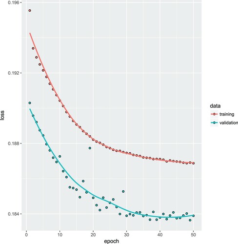
In Figure , we illustrate this preliminary analysis which shows that after roughly 40 epochs the model starts to over-fit to the training data (because the validation loss on
starts to increase). For this reason, we fix the early stopping rule at 40 epochs for all further network calibrations.
Figure 1. Preliminary analysis exploring the early stopping rule: model fitting on the training data (in upper graph) and tracking over-fitting on the validation data
(in lower graph); note that this is a standard output in Keras which (unfortunately) drops the factor 2 from the loss function (Equation7
(7)
(7) ), thus, the y-axis needs to be scaled with 2.
We then fit the FNN regression model over 40 epochs which provides us with an early stopped SGD calibration . Every SGD calibration needs an initial value in which the SGD algorithm is started from. This initial value is usually chosen at random, in Keras the default is the Glorot uniform initialiser, see Glorot and Bengio (Citation2010). This initialiser needs a seed for random number generation and, therefore, the early stopped SGD calibration
will depend on this initial seed. On lines (3a) –(3c) we provide three such early stopped SGD calibrations having different seeds 1, 2 and 3. We note that all three calibrations provide lower in-sample and out-of-sample losses on
and
, respectively, compared to the logistic regression model. This illustrates that the logistic regression model misses important model structure that is captured by the FNN. More worrying is that the balance property (Equation4
(4)
(4) ) fails to hold and the deviations are substantial, see last column of Table .
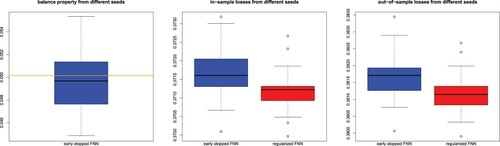
To receive a better intuition about the potential failure of the balance property, we run this SGD calibration over 50 different seeds (starting values of the SGD algorithm). On the left-hand side of Figure the box plot illustrates the different values we receive for . They fluctuate between 4.5% and 5.6% (the balance property is 5.007276%, orange horizontal line). We conclude that the balance property may substantially be misspecified by early stopping of SGD calibration which may lead to a huge bias and a severe global population (price) misspecification. In Figure (middle and right-hand side) we illustrate the resulting in-sample losses and the out-of-sample losses, respectively, over 50 different seeds of early stopped SGD calibrations. We note that the solutions provided on lines (3a) –(3c) of Table are part of these plots, i.e., they correspond to the first 3 seeds with corresponding values in Figure .
Figure 2. (lhs) Balance property (Equation4(4)
(4) ) of the early stopping FNN over 50 different seeds (starting points), the orange horizontal line shows the balance property of 5.007276%; (middle) in-sample learning losses on
and (rhs) out-of-sample test losses on
of the early stopping FNN (left box plots in graphs) and the GLM improved/regularised FNN (right box plots in graphs) over the 50 different seeds (starting values of the SGD algorithm).
5.4. Logistic regression bias regularisation
The failure of the balance property as illustrated in Figure (lhs) motivates us to apply the additional logistic regression step to the early stopping FNN calibration. This provides us with the GLM improved calibrations , see (Equation9
(9)
(9) ). Table , lines (4a)–(4c), provide the corresponding figures (they use exactly the same seeds as the ones on lines (3a)–(3c)). We note that in-sample losses on
decrease (which needs to be the case), that out-of-sample losses on
decrease (which shows that the early stopping FNN does not over-fit, yet), and that the balance property is fulfilled. The decreases in in-sample and out-of-sample losses are also illustrated in the red coloured box plots of Figure . From this example, we conclude that the GLM improved/regularised FNN calibration (Equation9
(9)
(9) ) provides a substantially improved FNN compared to (Equation8
(8)
(8) ), and this additional logistic regression step on the working data
should be explored for a suitable predictive model.
5.5. Shrinkage regularisation
Our final analysis explores the shrinkage regularisation approach of Section 4.2 by applying penalty term (Equation12(12)
(12) ). The use of this method is more complicated since it requires more work and fine-tuning. Firstly, we need to implement a custom-made loss function in Keras adding a KL divergence penalty term to the Bernoulli deviance loss. Secondly, we need to fine-tune the hyper-parameters: these are the batch size, the tuning parameter
and the number of epochs. We have performed a grid search to receive good parameters. We keep the batch size of 1000 samples and 40 epochs as in the previous calibrations. The tuning parameter is chosen as
.
In Table , we present the results. The general observation is that the shrinkage regularised versions are not fully competitive. Bias regularisation requires a comparably large tuning parameter η, and having a small batch size of 1000 this large tuning parameter η negatively impacts the accuracy of the FNN regression model. We conclude that the shrinkage regularisation approach is not fully compatible with SGD fitting because the bias property is a global property whereas SGD acts on (local) mini batches.
Table 2. Comparison of the homogeneous model (null model), the logistic regression model, the early stopping FNN and the GLM improved/regularised FNN, shrinkage regularised versions for different tuning parameters .
6. Conclusions
We have discussed the important problem of considering statistical models that provide unbiased mean estimates on a global population level (balance property). Classical statistical regression models like generalised linear model naturally have this balance property under the canonical link choice because the maximum likelihood estimator provides a critical value of the corresponding optimisation problem. In general, early stop gradient-descent calibrated neural networks fail to have the balance property, because early stopping prevents these models from taking parameters in critical points of the (deviance) loss function. In many applications, this does not reflect a favourable model calibration because it may lead to substantial price misspecification on a global population level. Therefore, we have proposed improvements that lead to globally unbiased solutions. These solutions include an additional generalised linear model optimisation step or shrinkage regularisation to empirical averages. The numerical example shows that we prefer the additional generalized linear model optimisation step.
Disclosure statement
No potential conflict of interest was reported by the author(s).
Additional information
Notes on contributors
Mario V. Wüthrich
Mario V. Wüthrich is Professor in the Department of Mathematics at ETH Zurich, Honorary Visiting Professor at City, University of London (2011-2022), Honorary Professor at University College London (2013-2019), and Adjunct Professor at University of Bologna (2014-2016). He holds a Ph.D. in Mathematics from ETH Zurich (1999). From 2000 to 2005, he held an actuarial position at Winterthur Insurance, Switzerland. He is Actuary SAA (2004), served on the board of the Swiss Association of Actuaries (2006-2018), and is Editor-in-Chief of ASTIN Bulletin (since 2018).
Notes
1 CASdatasets website http://cas.uqam.ca; see also page 55 of the reference manual CASdatasets Package Vignette (Citation2018); we use version 1.0-8 which has been packaged on 2018-05-20.
References
- Breiman, L. (2001). Statistical modeling: The two cultures. Statistical Science, 16(3), 199–231. https://doi.org/https://doi.org/10.1214/ss/1009213726
- Breiman, L., Friedman, J. H., Olshen, R. A., & Stone, C. J. (1984). Classification and regression trees. Wadsworth Statistics/Probability Series.
- Bühlmann, H., & Gisler, A. (2005). A course in credibility theory and its applications. Springer.
- CASdatasets Package Vignette (2018). Version 1.0-8, May 20, 2018. http://cas.uqam.ca
- Charpentier, A. (2015). Computational actuarial science with R. CRC Press.
- Cheng, X., Jin, Z., & Yang, H. (2020). Optimal insurance strategies: A hybrid deep learning Markov chain approximation approach. ASTIN Bulletin, 50(2), 449–477. https://doi.org/https://doi.org/10.1017/asb.2020.9
- Cox, D. R. (1958). The regression analysis of binary sequences. Journal of the Royal Statistical Society: Series B (Methodological), 20(2), 215–232. https://doi.org/https://doi.org/10.1111/j.2517-6161.1958.tb00292.x
- Cybenko, G. (1989). Approximation by superpositions of a sigmoidal function. Mathematics of Control, Signals, and Systems, 2(4), 303–314. https://doi.org/https://doi.org/10.1007/BF02551-274
- Gabrielli, A. (2020). A neural network boosted double overdispersed Poisson claims reserving model. ASTIN Bulletin, 50(1), 25–60. https://doi.org/https://doi.org/10.1017/asb.2019.33
- Glorot, X., & Bengio, Y. (2010). Understanding the difficulty of training deep feedforward neural networks. Proceedings of Machine Learning Research, 9, 249–256. Proceedings of the thirteenth international conference on artificial intelligence and statistics.
- Goodfellow, I., Bengio, Y., & Courville, A. (2016). Deep learning. MIT Press.
- Green, P. J. (1984). Iteratively reweighted least squares for maximum likelihood estimation, and some robust and resistant alternatives. Journal of the Royal Statistical Society: Series B (Methodological), 46(2), 149–170. https://doi.org/https://doi.org/10.1111/j.2517-6161.1984.tb01288.x
- Hornik, K., Stinchcombe, M., & White, H. (1989). Multilayer feedforward networks are universal approximators. Neural Networks, 2(5), 359–366. https://doi.org/https://doi.org/10.1016/0893-6080(89)90020-8
- LeCun, Y., Bengio, Y., & Hinton, G. (2015). Deep learning. Nature, 521(7553), 436–444. https://doi.org/https://doi.org/10.1038/nat-ure14539
- Lee, G. Y., Manski, S., & Maiti, T. (2020). Actuarial applications of word embedding models. ASTIN Bulletin, 50(1), 1–24. https://doi.org/https://doi.org/10.1017/asb.2019.28
- McCullagh, P., & Nelder, J. A. (1983). Generalized linear models. Chapman & Hall.
- Nelder, J. A., & Wedderburn, R. W. M. (1972). Generalized linear models. Journal of the Royal Statistical Society. Series A (General), 135(3), 370–384. https://doi.org/https://doi.org/10.2307/234-4614
- Noll, A., Salzmann, R., & Wüthrich, M. V. (2018). Case study: French motor third-party liability claims. SSRN Manuscript ID 3164764. Version March 4, 2020.
- Quinlan, J. R. (1992). Learning with continuous classes. In Proceedings of the 5th Australian joint conference on artificial intelligence (pp. 343–348). Singapore: World Scientific.
- Rumelhart, D. E., Hinton, G. E., & Williams, R. J. (1986). Learning representations by back-propagating errors. Nature, 323(6088), 533–536. https://doi.org/https://doi.org/10.1038/323-533a0
- Schmidhuber, J. (2015). Deep learning in neural networks: An overview. Neural Networks, 61, 85–117. https://doi.org/https://doi.org/10.1016/j.neunet.2014.09.003
- Shmueli, G. (2010). To explain or to predict? Statistical Science, 25(3), 289–310. https://doi.org/https://doi.org/10.1214/10-STS330
- Wang, C., Venkatesh, S. S., & Judd, J. S. (1994). Optimal stopping and effective machine complexity in learning. In Advances in neural information processing systems (NIPS'6) (pp. 303–310).
- Wang, Y., & Witten, I. H. (1997). Inducing model trees for continuous classes. In Proceedings of the ninth European conference on machine learning (pp. 128–137).
- Wüthrich, M. V., & Buser, C. (2016). Data analytics for non-life insurance pricing. SSRN Manuscript ID 2870308, Version of September 10, 2020.
- Wüthrich, M. V., & Merz, M. (2019). Editorial: Yes we CANN! ASTIN Bulletin, 49(1), 1–3. https://doi.org/https://doi.org/10.1017/asb.2018.42