Discussion on “on studying extreme values and systematic risks with nonlinear time series models and tail dependence measures”

Extreme value theory provides essential mathematical foundations for modelling tail risks and has wide applications. The emerging of big and heterogeneous data calls for the development of new extreme value theory and methods. For studying high-dimensional extremes and extreme clusters in time series, an important problem is how to measure and test for tail dependence between random variables. Section 3.1 of Dr. Zhang's paper discusses some newly proposed tail dependence measures. In the era of big data, a timely and challenging question is how to study data from heterogeneous populations, e.g. from different sources. Section 3.2 reviews some new developments of extreme value theory for maxima of maxima. The theory and methods in Sections 3.1 and 2.3 set the foundations for modelling extremes of multivariate and heterogeneous data, and we believe they have wide applicability. We will discuss two possible directions: (1) measuring and testing of partial tail dependence; (2) application of the extreme value theory for maxima of maxima in high-dimensional inference.

1. Partial tail dependence

Identifying the tail dependence between random variables can be helpful for determining appropriate multivariate extreme value distributions. Section 3.1 of Dr. Zhang's article reviews a series of work on tail dependence. Particularly, a test for tail independence based on the tail quotient correlation coefficient (TQCC) was introduced. The TQCC measurement has nice properties, including the simple interpretation and computation, and it has been successfully applied to financial risk studies, precipitation extremes, and so on. The method and theory are based on the assumption that $\{(X_i,Y_i),i=1,\dots ,n\}$ is a random sample of $(X,Y)$, and the aim is to study the tail dependence between X and Y. However, in some applications, both X and Y may depend on some other covariates Z. For example, Wang et al. (2012) showed that in the study of downscaling of precipitation, the coarser-resolution predictor variables generated from a global climate model can be used to predict the local extreme precipitations. For joint modelling and prediction of precipitation with other meteorological variables such as temperature, it will be important to assess the conditional tail dependence of these variables given Z, the global climate model outputs.

For any two random variables X and Y, which may not be identically distributed, the (upper) tail dependence index is defined as $\lambda =\underset{\tau \to 1}{lim}P\{Y>Q_{\tau }(Y)|X>Q_{\tau }(X)\},$where $Q_{\tau }(Y)$ and $Q_{\tau }(X)$ are the τth quantiles of Y and X, respectively. Dr. Zhang and his collaborators proposed the TQCC for measuring and testing the tail dependence. Suppose that there exist confounding variables Z which are likely to be related with X and Y, using the TQCC may lead to misleading conclusions. To account for the confounding factors, we can define the following partial tail dependence index ${\lambda }_{XY\cdot Z}(Z)=\underset{\tau \to 1}{lim}P\{Y>Q_{\tau }(Y|Z)|X>Q_{\tau }(X|Z)\},$where $Q_{\tau }(Y|Z)$ and $Q_{\tau }(X|Z)$ are the τth conditional quantiles of Y and X given Z, respectively. We conjecture that the index ${\lambda }_{XY\cdot Z}(Z)$ can capture the tail dependence between X and Y after accounting for the effect of Z. It would be interesting to study the interpretation and properties of ${\lambda }_{XY\cdot Z}$, together with its connections and distinctions from λ.

Suppose that we are interested in testing $H_0:{\lambda }_{XY\cdot Z}=0$ against the alternative hypothesis $H_a:{\lambda }_{XY\cdot Z}>0$. There are two possible ways to extend the TQCC-based method in Zhang et al. (2017) to test for the partial tail independence. Such tests can also be useful for the selection of orders in autoregressive models; see the discussion of quantile partial correlation in Li et al. (2015) for some related applications.

The first approach is a plug-in method. The idea is to remove the effects of Z on Y and X separately, and then assess the dependence of the estimated residuals. This approach will require specific forms for the two regression models. For instance, we may consider the following location-scale shift linear regression models, (1) $\begin{array}{rl}X& =Z^T{\beta }_1+(Z^T{\gamma }_1){ϵ}_1,\\ Y& =Z^T{\beta }_2+(Z^T{\gamma }_2){ϵ}_2,\end{array}$(1) where $({ϵ}_1,{ϵ}_2)$ are random errors, ${\beta }_j,{\gamma }_j$ are the unknown location and scale parameters, and $Z^T{\gamma }_j>0$, j = 1, 2. Given a random sample of $(X_i,Y_i,Z_i),i=1,\dots ,n$, we can estimate the parameters $({\beta }_j,{\gamma }_j)$ by $({\hat{\beta }}_j,{\hat{\gamma }}_j)$ using existing regression methods, for instance, the method in He (1997). Denote ${\widehat{ϵ}}_{1i}=(X_i-Z_i^T{\hat{\beta }}_1)/Z_i^T{\hat{\gamma }}_1$ and ${\widehat{ϵ}}_{2i}=(Y_i-Z_i^T{\hat{\beta }}_2)/Z_i^T{\hat{\gamma }}_2$. We can then define the partial tail quotient correlation coefficient as $\begin{array}{rl}{\mathrm{q}}_{n1}& =\frac{\begin{array}{c}\underset{1\le i\le n}{max}\{{\displaystyle \frac{max({\widehat{ϵ}}_{1i},u_n)}{max({\widehat{ϵ}}_{2i},u_n)}}-1\}\\ +\underset{1\le i\le n}{max}\{{\displaystyle \frac{max({\widehat{ϵ}}_{2i},u_n)}{max({\widehat{ϵ}}_{1i},u_n)}}-1\}\end{array}}{\begin{array}{c}\underset{1\le i\le n}{max}\left\{{\displaystyle \frac{max({\widehat{ϵ}}_{1i},u_n)}{max({\widehat{ϵ}}_{2i},u_n)}}\right\}\\ \times \underset{1\le i\le n}{max}\left\{{\displaystyle \frac{max({\widehat{ϵ}}_{2i},u_n)}{max({\widehat{ϵ}}_{1i},u_n)}}\right\}-1\end{array}},\end{array}$where $u_n$ is varying thresholds that tend to infinity. Under the model assumptions in (1(1) $\begin{array}{rl}X& =Z^T{\beta }_1+(Z^T{\gamma }_1){ϵ}_1,\\ Y& =Z^T{\beta }_2+(Z^T{\gamma }_2){ϵ}_2,\end{array}$(1) ), it can be shown that the partial tail dependence ${\lambda }_{XY\cdot Z}$ is the same as the tail dependence index between ${ϵ}_1$ and ${ϵ}_2$. One limitation of this approach is that it relies on the location-scale shift model assumption and thus may be susceptible to model misspecifications, though we can increase the flexibility by modelling the location and scale functions nonparametrically; see for instance (He, 1997; Keilegom & Wang, 2010; Pang et al., 2015).

The second approach is a quantile-regression-based method, which requires modelling the tail conditional quantiles of X and Y given Z. Let ${\hat{Q}}_{\tau }(X|Z)$ and ${\hat{Q}}_{\tau }(Y|Z)$ be the estimated conditional τth quantile of X and Y given Z, respectively, which can be obtained from either parametric (Wang et al., 2012) or semiparametric quantile regression (Xu et al., 2020). Then we can define a second version of the partial tail quotient correlation coefficient as $\begin{array}{r}{\mathrm{q}}_{n2}=\frac{\begin{array}{c}\underset{1\le i\le n}{max}\{{\displaystyle \frac{max(X_i,u_n(Z_i))}{max(Y_i,v_n(Z_i))}}-1\}\\ +\underset{1\le i\le n}{max}\{{\displaystyle \frac{max(Y_i,v_n(Z_i))}{max(X_i,u_n(Z_i))}}-1\}\end{array}}{\begin{array}{c}\underset{1\le i\le n}{max}\left\{{\displaystyle \frac{max(X_i,u_n(Z_i))}{max(Y_i,v_n(Z_i))}}\right\}\\ \times \underset{1\le i\le n}{max}\left\{{\displaystyle \frac{max(Y_i,v_n(Z_i))}{max(X_i,u_n(Z_i))}}\right\}-1\end{array}},\end{array}$where $u_n(Z)={\hat{Q}}_{\tau }(X|Z)$, $v_n(Z)={\hat{Q}}_{\tau }(Y|Z)$, and $\tau \to 1$ as $n\to \mathrm{\infty }.$

Similar to TQCC, the partial TQCC $q_{n1}$ and $q_{n2}$ can be used to test whether X and Y are tail independent after adjusting for the effect of Z. Theorem 4 in Zhang et al. (2017) establishes the limiting distribution of TQCC under $H_0:\lambda =0$. The measurement $q_{n1}$ assumes the location-scale shift models. If the location and scale functions are estimated consistently with a certain rate, we conjecture that ${\mathrm{q}}_{n1}$ has the similar asymptotic properties as $q_{u_n}$ in Zhang et al. (2017), so inference can be conducted by using the asymptotic ${\chi }^2$ distribution. The asymptotic properties of $q_{n2}$ would require more careful investigation.

We conduct a small simulation study by generating data from the following model: $\begin{array}{rl}{X}_i& =1+Z_i+{ϵ}_{i1},\\ Y_i& =1+2Z_i+(1+\gamma Z_i){ϵ}_{i2},i=1,\dots ,n,\end{array}$where ${ϵ}_{i2}=\sigma {ϵ}_{i1}+{ϵ}_{i3}$, ${ϵ}_{i1}$ and ${ϵ}_{i3}$ are independent standard Fréchet random variables, and $Z_i\sim U(0,1)$. We let n = 1000 and consider two cases: the homoscedastic case with $\gamma =0$ and heteroscedastic case with $\gamma =2$. The simulation is repeated 1000 times for each scenario. For $q_{n1}$, we take $u_n$ as the maximum of the 95th percentiles of the estimated residuals ${\widehat{ϵ}}_{i1}$ and ${\widehat{ϵ}}_{i2},i=1,\dots ,n$. For $q_{n2}$, we let $\tau =0.95$. Figure 1 plots the empirical density of $T_n=2n\{1-\exp (-1/u_n)q_{n1}$ obtained under the null model with $\sigma =0$ and the density of ${\chi }^2(4)$. Results show that, as in Theorem 3.8 of Dr. Zhang's paper for $q_{u_n}$, ${\chi }^2(4)$ provides a good approximation to the normalised $q_{n1}$ under $H_0$. 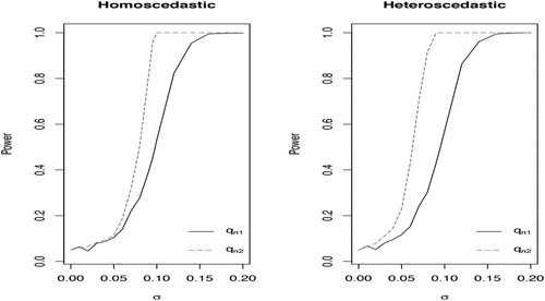Figure 2 plots the power curves of tests based on $q_{n1}$ and $q_{n2}$ using the Monte Carlo critical values against σ. The power of both tests increases gradually with σ, while $q_{n2}$ exhibits higher power than $q_{n1}$ for detecting the partial tail dependence. It would be interesting to further study the theoretical and empirical properties of $q_{n2}$.

Figure 1. The empirical density of $T_n=2n\{1-\exp (-1/u_n)\}{q}_{n1}$ under $H_0$ and the density of ${\chi }^2(4)$.

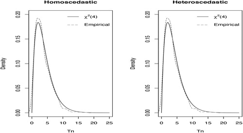
Figure 2. Power of tests based on $q_{n1}$ and $q_{n2}$ for testing the partial tail independence between X and Y given Z.

2. Maxima of maxima for high-dimensional inference

In Section 3.2, Dr. Zhang introduces some newly developed extreme value theory for the maxima of k maxima, from either different variables or subsequences of the same variable. Denote $M_{l,n_l}=max\{Y_{l,1},\dots ,Y_{l,n_l}\}$, $l=,\dots ,k$ and $M_n=max(M_{1,n_1},\dots ,M_{k,n_k})$. Section 3.2 reviews some new results for the limiting distribution of $M_n$. We believe such results would be very useful for high-dimensional inference with multivariate responses.

Maximum-type statistics and extreme value theory have been used in many high-dimensional inference problems. Some examples include testing for high-dimensional mean differences (Cai et al., 2014; Xu et al., 2016), inference on high-dimensional correlation matrix (Jiang, 2004; Xiao & Wu, 2013), testing and identification of significant predictors (Tang & Pan, 2020), just to name a few. In these works, the test statistics are defined as the maximum of a high-dimensional independent or dependent random variables, e.g., the sample correlations (Jiang, 2004) or the normalised squared differences of sample covariances of p variables from two populations (Cai et al., 2013), the squared sample mean differences of p variables from two populations (Cai et al., 2014), or the squared score statistics capturing the impacts of p predictors on the response variable (Tang & Pan, 2020; Wu et al., 2019), where p is often larger than the sample size n. The hypothesis testing is then conducted by using the limiting distribution of the maximum-type statistic, that is, the Type I extreme value distribution. One typical application is in genome-wide association studies, where one main interest is in comparing the means or covariances of a large number of single nucleotide polymorphisms (SNPs) between treatment and control, or detecting possible associations between a phenotype or disease and gene pathways.

In some applications, the researcher may be interested in assessing the association between p SNPs and multiple diseases or phenotypes jointly. The new extreme value theory of maxima of maxima in Dr. Zhang's work could be helpful to develop valid testing procedures for such applications. For simplicity, we will use k = 2 to illustrate the possible application in this context. Let $S_{l,j,n}^2$ denote the squared normalised score test statistic measuring the effect of the jth SNP on the lth phenotype, where $j=1,\dots ,p$ and l = 1, 2. Under some regularity conditions, it can often be shown that $S_{l,j,n}$ are asymptotically normal variables that are likely to be correlated. Suppose that we want to test the null hypothesis $H_0$: none of the SNPs from a gene pathway is associated with the two phenotypes against the alternative $H_A$: there exists at least one SNP that has an association with either or both phenotypes. One natural test statistic is $\begin{array}{rl}{M}_n& =max(M_{1,n},M_{2,n}),\mathrm{where}\\ M_{l,n}& =\underset{j=1,\dots ,p}{max}{S}_{l,j,n}^2,l=1,2,\end{array}$and we would reject $H_0$ with large $M_n$. Theorem 3.11 in Dr. Zhang's work can help determine the critical value or calculate the p-value. Let $F_1$ and $F_2$ be the cumulative distributions of $S_{1,j,n}^2$ and $S_{1,j,n}^2$ for $j=1,\dots ,p$. In this context, $F_1$ and $F_2$ are approximately ${\chi }^2(1)$ distribution under $H_0$. Let $m_{1,n}$ and $m_{2,n}$ be the observed values of $M_{1,n}$ and $M_{2,n}$. Define $m_n=max\{m_{1,n},m_{2,n}\}$. Then based on Theorem 3.11, we can approximate the p-value with (2) $\begin{array}{rl}p-\mathrm{val}& =P(M_n>m_n|H_0)\\ & =P(M_{1,n}>m_n,M_{2,n}>m_n|H_0)\\ & \approx 1-e^{-{\tau }_1-{\tau }_2},\end{array}$(2) where ${\tau }_1=n\{1-F_1(m_{1,n})\}$ and ${\tau }_2=n\{1-F_2(m_{2,n})\}$.

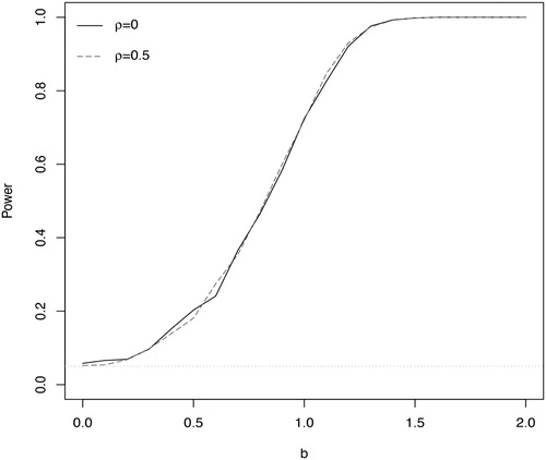
We conduct a small simulation study to try out this idea. We generate $S_{1,j,n}$ and $S_{2,j,n}$ from the bivariate normal distribution with means b, unit variance and correlation ρ, where $j=1,\dots ,p=1000.$ Figure 3 shows the power curves of this test against b for $\rho =0$ and 0.5. The simulation results suggest the test based on the extreme value theory for maxima of maxima performs well: the type I error is controlled around the nominal level of 0.05, and the power increases gradually with the signal b. However, as mentioned above, in the GWAS applications, $S_{l,j,n}$ are often correlated across l and $j=1,\dots ,p$, so further research is needed to provide rigorous justification for applying the maxima of maxima theory to the multivariate high dimensional inference problems.

Figure 3. Power curve of the test based on the maxima of maxima theory for high-dimensional inference with two phenotype. The parameter ρ corresponds to the correlation used in the simulation. The x-axis represents the deviation from the null hypothesis. The horizontal line dotted corresponds to the 0.05 nominal level.

Acknowledgments

We congratulate Dr. Zhang for a stimulating and interesting article on the important topics of extreme values with nonlinear time series models and tail dependence measures and thank Professor Jun Shao for giving us the opportunity to discuss this work.

Disclosure statement

No potential conflict of interest was reported by the author(s).

Additional information

Notes on contributors

Wen Xu

Wen Xu is a Phd candidate of Fudan University.

Huixia Judy Wang

Huixia Judy Wang is a Professor of The George Washington University.

References

- Cai, T. T., Liu, W., & Xia, Y. (2013). Two-sample covariance matrix testing and support recovery in high-dimensional and sparse settings. Journal of the American Statistical Association, 108, 265–277. https://doi.org/10.1080/01621459.2012.758041
- Cai, T. T., Liu, W., & Xia, Y. (2014). Two-sample test of high dimensional means under dependence. Journal of the Royal Statistical Society, Series B, 76, 349–372. https://doi.org/10.1111/rssb.2014.76.issue-2
- He, X. (1997). Quantile curves without crossing. The American Statistician, 51(2), 186–192. https://doi.org/10.1080/00031305.1997.10473959
- Jiang, T. (2004). The asymptotic distributions of the largest entries of sample correlation matrices. The Annals of Applied Probability, 14(2), 865–880. https://doi.org/10.1214/105051604000000143
- Keilegom, I. V., & Wang, L. (2010). Semiparametric modeling and estimation of heteroscedasticity in regression analysis of cross-sectional data. Electronic Journal of Statistics, 4, 186–192. https://doi.org/10.1214/09-EJS547
- Li, G., Li, Y., & Tsai, C. (2015). Quantile correlations and quantile autoregressive modeling. Journal of the American Statistical Association, 110(509), 246–261. https://doi.org/10.1080/01621459.2014.892007
- Pang, L., Lu, W., & Wang, H. (2015). Local Buckley-James estimator for the heteroscedastic accelerated failure time model. Statistica Sinica, 25, 863–877. https://doi.org/10.5705/ss.2013.313
- Tang, Y., & Pan, Q. (2020). Conditional marginal test for high dimensional quantile regression. Statistica Sinica. to appear.
- Wang, H., Li, D., & He, X. (2012). Estimation of high conditional quantiles for heavy-tailed distributions. Journal of the American Statistical Association, 107, 1453–1464. https://doi.org/10.1080/01621459.2012.716382
- Wu, C., Xu, G., & Pan, W. (2019). An adaptive test on high-dimensional parameters in generalized linear models. Statistica Sinica, 28, 1226–1255. https://doi.org/10.5705/ss.202017.0354
- Xiao, H., & Wu, W. (2013). Asymptotic theory for maximum deviations of sample covariance matrix estimates. Stoch Process and Their Applications, 123(7), 2899–2920. https://doi.org/10.1016/j.spa.2013.03.012
- Xu, W., Li, D., & Wang, H. (2020). Extreme quantile estimation based on the tail single-index model. Statistica Sinica. https://doi.org/10.5705/ss.202020.0051
- Xu, G., Lin, L., Wei, P., & Pan, W. (2016). An adaptive two-sample test for high-dimensional means. Biometrika, 103(3), 609–624. https://doi.org/10.1093/biomet/asw029
- Zhang, Z., Zhang, C., & Cui, Q. (2017). Random threshold driven tail dependence measures with application to precipitation data analysis. Statistica Sinica, 27(2), 421–453. https://doi.rog/10.5705/ss.202014.0421