Stochastic loss reserving using individual information model with over-dispersed Poisson

Abstract

For stochastic loss reserving, we propose an individual information model (IIM) which accommodates not only individual/micro data consisting of incurring times, reporting developments, settlement developments as well as payments of individual claims but also heterogeneity among policies. We give over-dispersed Poisson assumption about the moments of reporting developments and payments of every individual claims. Model estimation is conducted under quasi-likelihood theory. Analytic expressions are derived for the expectation and variance of outstanding liabilities, given historical observations. We utilise conditional mean square error of prediction (MSEP) to measure the accuracy of loss reserving and also theoretically prove that when risk portfolio size is large enough, IIM shows a higher prediction accuracy than individual/micro data model (IDM) in predicting the outstanding liabilities, if the heterogeneity indeed influences claims developments and otherwise IIM is asymptotically equivalent to IDM. Some simulations are conducted to investigate the conditional MSEPs for IIM and IDM. A real data analysis is performed basing on real observations in health insurance.

Keywords:

• Risk management
• loss reserving
• individual information model
• over-dispersed Poisson
• quasi-likelihood
• MSEP

1. Introduction

In the background of stochastic reserving, loss reserving is referred to a procedure to predict incurred outstanding liabilities in general insurance companies. It is well known that chain-ladder method proposed by Mack (1993) and its related versions can be easily performed by using pencil and paper because of the simple aggregate data structure called run-off triangle and hence are popular in practice. However, as England and Verrall (2002) mentioned, the advantages of aggregate data models are at the cost of prediction accuracy because of information loss caused by simply aggregating individual or micro data, which records incurring time, reporting time, settlement time as well as payment processes of individual claims. In risk management of insurance companies, with the modern computer technology, it is urgent for actuaries to explore the usage of related information to improve the accuracy in predicting the liabilities, which also attracts increasing interests of many scholars from actuarial science. Antonio and Plat (2014), Pigeon et al. (2013, 2014) demonstrated by an empirical analysis that loss reserving based on individual data had more prediction accuracy than aggregate models. Huang, Qiu, Wu, Zhou (2015), Huang, Qiu, Wu (2015) and Huang et al. (2016) revealed that individual loss reserving had more accuracy than methods using aggregate data in sense that the former produced a smaller mean square error.

A small stream of earlier literature about IDMs, for example, Arjas (1989) and Norberg (1993, 1999) formulated a probabilistic framework for the developments of individual claims. Most recently, Yu and He (2016) modelled the individual claim development process by marked Cox processes (also known as double stochastic processes). As we all know, it is challenging to acquire analytic expressions for the moments of outstanding liabilities under continuous-time IDMs. Perhaps partly for this reason, there is a great deal of work that has been done under discrete-time IDMs, see, e.g., Pigeon et al. (2013, 2014), Verrall et al. (2010), Huang, Qiu, Wu, Zhou (2015), Huang, Qiu, Wu (2015) and Huang et al. (2016). Zhao and Zhou (2010) considered the R-delays so as to predict the incurred but not settled outstanding liabilities. Unfortunately, IDMs also confront information loss caused by neglecting individual information, i.e., information from policy or policyholder. It is not clear so far how much accuracy in predicting the outstanding liabilities is sacrificed, when the individual information is neglected. In the present paper, we will explore how much improvement in the accuracy that will be measured by conditional MSEP can be achieved by incorporating the useful individual information into modelling under discrete time framework similar as Huang, Qiu, Wu, Zhou (2015), Huang, Qiu, Wu (2015) and Huang et al. (2016). Besides, we avoid the strong Poisson distribution assumption for the number of individual claims assumed in Huang, Qiu, Wu, Zhou (2015), Huang, Qiu, Wu (2015) and Huang et al. (2016) and instead extend to weak assumptions about the first two moments so that parameters estimation can be conducted under quasi-likelihood theory (cf. McCullagh & Nelder, 1989).

The conditional MSEP is broadly used to compare different models for loss reserving. It is well known that the conditional MSEP is the sum of process variance caused by the randomness of outstanding liabilities and estimation error originating from uncertainty of parameters estimators. It is theoretically feasible to estimate it by bootstrap method. There were some examples which discussed the MSEP under collective models – for instance, Mack (1993), Mack (2000) (comparing three methods – Benktander, Bornhuetter–Ferguson and chain-ladder under the criteria of MSEP), Alai et al. (2009, 2010) (Bornhuetter–Ferguson method under generalised linear model) and Wüthrich and Merz (2008) (comprehensive summary of the details of methods based on aggregate data). Besides, Lindholm et al. (2020) introduced a semi-analytic approximation method to estimate the conditional MSEP, where the method is illustrated by loss reserving based on aggregate data. Examples that have applied the approximation method are Wahl (2019), who computed explicit moments of outstanding liabilities by applying discretisation scheme under the framework of Antonio and Plat (2014), and Wahl et al. (2019) who modelled individual data on aggregate level. In the present paper, we also use the approximation method for the MSEP, which is derived under IIM, because of its simplification.

The paper is organised as follows. In Section 2, we describe the data structure and display the mathematical expression of outstanding liabilities caused by a risk portfolio at a given evaluation date. In Section 3, we separately model reporting developments, settlement delays and payments of claims and in each part, we formulate the model assumptions as well as estimation for the model parameters. Section 4 mainly derives the formulas of loss reserve and conditional variance of outstanding liabilities given historical observations, and studies the improvement of accuracy achieved by IIM with respect to IDM. Section 5 reports some simulation results and a real data analysis. Section 6 concludes the paper with a few remarks.

2. Data structure

Claim events incurred by some policy are usually reported to the insurer in some time periods (reporting delays) after their occurrence and the reported claims are finally settled with some time lags (settlement delays) between their reports and final settlements. Before going further, it is necessary to discuss the supports of reporting and settlement delays. In the following assumption, we assume that there exists maximum reporting delay $D^r$ and settlement delay $D^s$. Actually, there are basically two cases for the supports of the delays: finite and infinite. It would be a known priori (generally read from the items of the insurance contracts) if the supports are finite or infinite before any loss reserving is taken care of. Even for the case the delays take unrestricted values, if the probability to take values over certain limits is quite small, one can safely assume a capped delays by cutting off the tails with probability small enough. As a result, the assumption of capped delays is reasonable in many real insurance businesses, especially for such insurance without very much high claims payments. An example is the general health insurance. The assumption of capped delays has been extensively adopted in such traditional methods as chain-ladder algorithm. If the tails cannot be safely cut off, however, the models such as the one proposed in Crevecoeur et al. (2019) or some others would be more suitable. From the statistical point of view, for their distributions to be reasonably estimated with observations over a finite number of years, at least one of the two assumptions is necessary: they take only a finite number of values with arbitrary probabilities (but subject to normalisation) or countably infinitely many values but with their distribution functions identified by finite many parameters. Whatever the case, the number of unknown parameters that need to be estimated must be finite. Here the former is taken, whereas Crevecoeur et al. (2019), for example, took the latter.

Then we specify the data structure used in our model. It is in discrete time version as, e.g., Huang, Qiu, Wu (2015) did. Typically, the data for modelling is organised through periods with fixed length such as 1 year, one season or 1 month depending on lines of business. Conventionally, those periods are referred to ‘(accident) years’. This is also a way widely adopted by insurers to predict the incurred outstanding liabilities in practice. Specifically, the whole observation horizon is made of n accident years and loss reserving is evaluated at the end of nth accident year. In year i, $i=1,2,\dots ,n$, there are $m_i$ insurance policies, each of which is coded by $(i,k)$, $k=1,2,\dots ,m_i$.

Every individual $(i,k)$ is associated with a random risk exposure $r_{ik}$ and d-dimensional vector of covariate ${\mathit{x}}_{ik}$ whose first entry is 1 and other entries indicating the individual information/features that influence the developments of individual claims. The developments of claims incurred by individual $(i,k)$ are detailed as follows.

1. The reporting developments of claims are recorded by $N_{iku}^r$, $u=0,1,\dots ,D^r$, where $N_{iku}^r$ is the number of claims which are incurred in year i and reported in year i + u.

2. For $N_{iku}^r$ claims, $u=0,1,\dots ,D^r$, their settlement developments are tracked by $N_{ikuv}$, $v=0,1,\dots ,D^s$, where $N_{ikuv}$ is the number of claims which are reported in year i + u and settled in year i + u + v.

3. Payments for each claim are assumed to be paid for only once at its final settlement. For $N_{ikuv}$ claims, $u=0,1,\dots ,D^r,v=0,1,\dots ,D^s$, we use $Y_{ikuvl}$, $l=1,2,\dots ,N_{ikuv}$ to record corresponding payments.

Then the random element associated with individual $(i,k)$ is denoted by $\begin{array}{r}\{r_{ik},{\mathit{x}}_{ik};\{N_{iku}^r;(N_{ikuv};(Y_{ikuvl}{)}_{l=1}^{N_{ikuv}}{)}_{v=0}^{D^s}{\}}_{u=0}^{D^r}\},\end{array}$$i=1,\dots ,n,k=1,\dots ,m_i$, which are i.i.d. from the population $\begin{array}{r}\{r,\mathit{x};\{N_u^r;(N_{uv};(Y_{uvl}{)}_{l=1}^{N_{uv}}{)}_{v=0}^{D^s}{\}}_{u=0}^{D^r}\},\end{array}$which can be considered as a complete observation of a representative policy in year i.

Following conventional terms, a claim, which has been reported to the insurer but not settled, is known as RBNS claim and a claim, which has been incurred but not reported to the insurer, is known as IBNR claim. For accident year i, the individual observed data is as follows.

1. The reporting developments of a representative policy in year i are truncated in sense that we can only observe ${\mathcal{F}}^r=\{N_0^r,N_1^r,\dots ,N_{D_i^r}^r\}$, where (1) $\begin{array}{r}{D}_i^r=D^r\wedge (n-i),\end{array}$(1) represents the largest reporting delays of the reported claims in accident year i.

2. For $N_u^r$ reported claims, $u=0,1,\dots ,D_i^r$, their settlement developments are censored in sense that we can observe $\{N_{u0},N_{u1},\dots ,N_{u{D}_{i+u}^s},N_u^{rbns}\}$, where (2) $\begin{array}{r}{D}_{i+u}^s=D^s\wedge (n-i-u),\end{array}$(2) is the largest settlement delays of settled claims with reporting delay u in accident year i and the number $N_u^{rbns}:=\sum _{v=n-i-u+1}^{D^s}{N}_{uv}$, which is the number of RBNS claims with reporting delays u. Note that $N_u^{rbns}=0$ if $n-i-u\ge D^s$. Denote by ${\mathcal{F}}^s=\bigcup _{u=0}^{D_i^r}\{N_{u0},N_{u1},\dots ,N_{u{D}_{i+u}^s},N_u^{rbns}\}$.

3. For $N_{uv}$ settled claims, $u=0,1,\dots ,D_i^r,v=0,1,\dots ,D_{i+u}^s$, the observed payments for them are gathered in set $\{Y_{uv1},Y_{uv2},\dots ,Y_{uv{N}_{uv}}\}$. Denote ${\mathcal{F}}^p=\bigcup _{u=0}^{D_i^r}\bigcup _{v=0}^{D_{i+u}^s}\{Y_{uv1},Y_{uv2},\dots ,Y_{uv{N}_{uv}}\}$.

Then individual observation ${\mathcal{F}}^o$ is the union of $\{r,\mathit{x}\}$, ${\mathcal{F}}^r$, ${\mathcal{F}}^s$ and ${\mathcal{F}}^p$, that is $\begin{array}{r}{\mathcal{F}}^o=\{r,\mathit{x}\}\cup {\mathcal{F}}^r\cup {\mathcal{F}}^s\cup {\mathcal{F}}^p\end{array}$and the historical observations of all policies in the portfolio, denoted by ${\mathcal{F}}^{uo}$, is just the union of policy-specified observation that is ${\mathcal{F}}^{uo}=\bigcup _{i=1}^n\bigcup _{k=1}^{m_i}{\mathcal{F}}_{ik}^o$, where ${\mathcal{F}}_{ik}^o$ is the policy-specified realisations of ${\mathcal{F}}^o$ in year i that is $\begin{array}{r}{\mathcal{F}}_{ik}^o=\{r_{ik},{\mathit{x}}_{ik}\}\cup {\mathcal{F}}_{ik}^r\cup {\mathcal{F}}_{ik}^s\cup {\mathcal{F}}_{ik}^p.\end{array}$

It is well known that RBNS and IBNR claims of the risk portfolio naturally result in outstanding liabilities to the insurer. Specifically, the total of future payments for all the RBNS and IBNR claims can be represented as (3) $\begin{array}{r}R:=\sum _{i=1}^n{R}_i^{rbns}+\sum _{i=1}^n{R}_i^{ibnr},\end{array}$(3) where $\begin{array}{rl}{R}_i^{rbns}& =\sum _{k=1}^{m_i}\sum _{u=0}^{D_i^r}\sum _{v=n-i-u+1}^{D^s}\sum _{l=1}^{N_{ikuv}}{Y}_{ikuvl}\text{and}\\ R_i^{ibnr}& =\sum _{k=1}^{m_i}\sum _{u=n-i+1}^{D^r}\sum _{v=0}^{D^s}\sum _{l=1}^{N_{ikuv}}{Y}_{ikuvl},\end{array}$are RBNS and IBNR liabilities incurred in year i, respectively. Thoroughly, we take the convention $\sum _{j=j_1}^{j_2}\cdot =0$ if $j_1>j_2$.

3. Model specification

This section separately specifies the models for the reporting developments, settlement developments and payments of claims. In each part, we first give model assumptions and then detail the parameter estimations under both IIM and IDM. The model assumptions in this section are all given under the condition that risk exposure r and covariates $\mathit{x}$ are known.

3.1. Modelling reporting developments of claims

Model assumption for reporting developments of claims is given as follows. It is mainly about the first and second moments of reporting developments of claims. The assumption involves vectors of parameters $\text{β},{\mathit{\pi }}_1,{\mathit{\pi }}_2,\dots ,{\mathit{\pi }}_{D^r}$, which are all d-dimensional vector.

Assumption 3.1

For an individual with $(r,\mathit{x}),$ assume that $N_u^r,$ $u=0,1,\dots ,D^r$ are independent, $\mathbb{E}[N_u^r|r,\mathit{x}]=r{\lambda }_u$ and $\mathrm{V}\mathrm{a}\mathrm{r}(N_u^r|r,\mathit{x})=\varphi r{\lambda }_u,$ where ${\lambda }_u=\lambda p_u$ with $\lambda =\exp \left({\mathit{x}}^{\prime }\text{β}\right)$ and $p_u(\mathit{\pi };\mathit{x})=\frac{\exp \left({\mathit{x}}^{\mathrm{\prime }}{\mathit{\pi }}_u\right)}{\sum _{j=0}^{D^r}\exp \left({\mathit{x}}^{\mathrm{\prime }}{\mathit{\pi }}_j\right)}$, ${\mathit{\pi }}_0=\mathbf{0}$ as well as ${\mathit{\pi }}^{\prime }=({\mathit{\pi }}_1^{\prime },{\mathit{\pi }}_2^{\prime },\dots ,{\mathit{\pi }}_{D^r}^{\prime })$.

Remark 3.1

In order to make $\mathit{\pi }$ be reasonably estimated, the condition $n>D^r$ is necessary.

By independence among policies and assumption above, one can construct the quasi-likelihood function of reported claims as follows, (4) $\begin{array}{r}{Q}^r(\text{β},\mathit{\pi })=\frac{1}{\varphi }\sum _{i=1}^n\sum _{k=1}^{m_i}\sum _{u=0}^{D_i^r}(N_{iku}^r\log {\lambda }_{iku}-r_{ik}{\lambda }_{iku}),\end{array}$(4) where ${\lambda }_{iku}$ is policy-specified quantities of ${\lambda }_u$ that is $\begin{array}{r}{\lambda }_{iku}={\lambda }_{ik}{p}_{iku}=\exp \left({\mathit{x}}_{ik}^{\prime }\text{β}\right)\cdot \frac{\exp \left({\mathit{x}}_{ik}^{\mathrm{\prime }}{\mathit{\pi }}_u\right)}{\sum _{j=0}^{D^r}\exp \left({\mathit{x}}_{ik}^{\mathrm{\prime }}{\mathit{\pi }}_j\right)}.\end{array}$One can refer to McCullagh and Nelder (1989) for more details about quasi-likelihood theory. Similar to maximum likelihood estimation, parameters $(\text{β},\mathit{\pi })$ can be estimated by maximising $Q^r(\text{β},\mathit{\pi })$ with respect to the parameters. Denote by $\mathit{\lambda }=\mathrm{v}\mathrm{e}\mathrm{c}(r_{ik}{\lambda }_{iku},i=1,\dots ,n,k=1,\dots ,m_i,u=0,\dots ,D_i^r)$ and stack $N_{iku}^r$s as a vector ${\mathit{N}}^r$ such that entry $N_{iku}$ is corresponding to $r_{ik}{\lambda }_{iku}$ in vector $\mathit{\lambda }$. The quasi-score function, i.e., partial derivatives of $Q^r(\text{β},\mathit{\pi })$ with respect to the parameters is (5) $\begin{array}{r}\mathrm{\nabla }{Q}^r(\text{β},\mathit{\pi }):=\frac{\mathrm{\partial }{Q}^r(\text{β},\mathit{\pi })}{\mathrm{\partial }({\text{β}}^{\prime },{\mathit{\pi }}^{\prime }{)}^{\prime }}=\frac{1}{\varphi }{X}^{r\mathrm{\prime }}\mathrm{d}\mathrm{i}\mathrm{a}\mathrm{g}\left(\mathit{\lambda }{)}^{-1}\right({\mathit{N}}^r-\mathit{\lambda }),\end{array}$(5) where $X^r=\frac{\mathrm{\partial }\mathit{\lambda }}{\mathrm{\partial }({\text{β}}^{\prime },{\mathit{\pi }}^{\prime })}$. To determine the block entries of $X^r$, one needs the unit vector ${\mathit{\delta }}_s$ with 1 at component s (any positive integer) and ${\mathit{\delta }}_0=\mathbf{0}$, of which dimensions can be read from context, and the following partial derivatives $\begin{array}{r}{r}_{ik}\cdot \frac{\mathrm{\partial }{\lambda }_{iku}}{\mathrm{\partial }({\text{β}}^{\prime },{\mathit{\pi }}^{\prime })}=r_{ik}{\lambda }_{iku}{\left(\begin{array}{c}1\\ {\mathit{\delta }}_u-{\mathit{p}}_{ik}\end{array}\right)}^{\prime }\otimes {\mathit{x}}_{ik}^{\prime },\end{array}$where ${\mathit{p}}_{ik}=(p_{ik1},p_{ik2},\dots ,p_{ik{D}^r}{)}^{\prime }$ and ⊗ is the Kronecker product.

The covariance matrix of $\mathrm{\nabla }{Q}^r(\text{β},\mathit{\pi })$, which is also the negative expected value of $\frac{\mathrm{\partial }\mathrm{\nabla }{Q}^r(\text{β},\mathit{\pi })}{\mathrm{\partial }({\text{β}}^{\prime },{\mathit{\pi }}^{\prime })}$, is (6) $\begin{array}{r}{I}^r(\text{β},\mathit{\pi })=\frac{1}{\varphi }{X}^{r\mathrm{\prime }}\mathrm{d}\mathrm{i}\mathrm{a}\mathrm{g}(\mathit{\lambda }{)}^{-1}{X}^r.\end{array}$(6) The parameters $(\text{β},\mathit{\pi })$ are estimated by Newton–Raphson with Fisher scoring starting with initials $({\text{β}}^{\mathrm{o}\mathrm{l}\mathrm{d}},{\mathit{\pi }}^{\mathrm{o}\mathrm{l}\mathrm{d}})$ and updating estimated parameters in the following way: $\begin{array}{rl}& ({\text{β}}^{\mathrm{n}\mathrm{e}\mathrm{w}\mathrm{\prime }},{\mathit{\pi }}^{\mathrm{n}\mathrm{e}\mathrm{w}\mathrm{\prime }}{)}^{\prime }=({\text{β}}^{\mathrm{o}\mathrm{l}\mathrm{d}\mathrm{\prime }},{\mathit{\pi }}^{\mathrm{o}\mathrm{l}\mathrm{d}\mathrm{\prime }}{)}^{\prime }\\ & +\left(X_0^{r\mathrm{\prime }}\mathrm{d}\mathrm{i}\mathrm{a}\mathrm{g}\right({\mathit{\lambda }}_0{)}^{-1}{X}_0^r{)}^{-1}{X}_0^{r\mathrm{\prime }}\mathrm{d}\mathrm{i}\mathrm{a}\mathrm{g}\left({\mathit{\lambda }}_0{)}^{-1}\right({\mathit{N}}^r-{\mathit{\lambda }}_0),\end{array}$where $X_0^r$ and ${\mathit{\lambda }}_0$ are obtained by replacing $(\text{β},\mathit{\pi })$ with $({\text{β}}^{\mathrm{o}\mathrm{l}\mathrm{d}},{\mathit{\pi }}^{\mathrm{o}\mathrm{l}\mathrm{d}})$. Write the estimated parameters as $(\widehat{\text{β}},\hat{\mathit{\pi }})$. To estimate dispersion parameter ϕ, we adopt conventional method–moment estimation that is, $\begin{array}{rl}\hat{\varphi }& =\frac{1}{\sum _{u=0}^{D^r}\sum _{i=1}^{n-u}{m}_i-(D^r+1)p}\\ & \times \sum _{u=0}^{D^r}\sum _{i=1}^{n-u}\sum _{k=1}^{m_i}\frac{(N_{iku}^r-r_{ik}{\hat{\lambda }}_{iku}{)}^2}{r_{ik}{\hat{\lambda }}_{iku}},\end{array}$where ${\hat{\lambda }}_{iku}$s are plug-in estimates of ${\lambda }_{iku}$ that is $\begin{array}{r}{\hat{\lambda }}_{iku}=\exp \left({\mathit{x}}_{ik}^{\prime }\widehat{\text{β}}\right)\cdot \frac{\exp \left({\mathit{x}}_{ik}^{\mathrm{\prime }}{\hat{\mathit{\pi }}}_u\right)}{\sum _{j=0}^{D^r}\exp \left({\mathit{x}}_{ik}^{\mathrm{\prime }}{\hat{\mathit{\pi }}}_j\right)}.\end{array}$IDM considers that policy's feature information has no effect on reporting developments that is the coefficients of $x_1,x_2,\dots ,x_{d-1}$ are thought to be zero. Obviously, IDM is a misspecified model if the feature information indeed influence those developments. Therefore, in IDM, λ and $p_u$ are thought to keep fixed among all policies and then ${\lambda }_u$ is same for the policies. By maximising function $Q^r$ in (4(4) $\begin{array}{r}{Q}^r(\text{β},\mathit{\pi })=\frac{1}{\varphi }\sum _{i=1}^n\sum _{k=1}^{m_i}\sum _{u=0}^{D_i^r}(N_{iku}^r\log {\lambda }_{iku}-r_{ik}{\lambda }_{iku}),\end{array}$(4) ) with respect to ${\lambda }_u$, one can obtain that (7) $\begin{array}{r}{\hat{\lambda }}_u=\frac{{\tilde{N}}_u^r}{r_{\left(u\right)}},u=0,1,\dots ,D^r,\end{array}$(7) where ${\tilde{N}}_u^r=\sum _{i=1}^{n-u}\sum _{i=1}^{m_i}{N}_{iku}^r$ representing total number of reported claims with reporting delay u and $r_{\left(u\right)}=\sum _{i=1}^{n-u}\sum _{i=1}^{m_i}{r}_{ik}$ meaning total exposures in the first n−u years.

3.2. Modelling settlement delays

In IIM, the settlement developments of individual claims after their reporting to the insurer have the following assumption. The assumption involves vectors of parameters ${\mathit{\rho }}_1,{\mathit{\rho }}_2,\dots ,{\mathit{\rho }}_{D^r}$, which are all d-dimensional vector.

Assumption 3.2

Assume that given $N_u^r,$ $(N_{u0},N_{u1},\dots ,N_{u{D}^s})$ follows multinomial distribution with parameters $N_u^r$ and $(q_0,\dots ,q_{D^s}),$ where $\begin{array}{r}{q}_v(\mathit{\rho };\mathit{x})=\frac{\exp \left({\mathit{x}}^{\prime }{\mathit{\rho }}_v\right)}{\sum _{j=0}^{D^s}\exp \left({\mathit{x}}^{\prime }{\mathit{\rho }}_j\right)},v=0,\dots ,D^s,\end{array}$ with ${\mathit{\rho }}_0=\mathbf{0}$, as well as ${\mathit{\rho }}^{\prime }=({\mathit{\rho }}_1^{\prime },{\mathit{\rho }}_2^{\prime },\dots ,{\mathit{\rho }}_{D^s}^{\prime })$ and the tuples $(N_{u0},N_{u1},\dots ,N_{u{D}^s}),u=0,\dots ,D^r$ are independent.

Remark 3.2

Similar to the condition in Remark 3.1, the condition $n>D^s$ is necessary to make $\mathit{\rho }$ be reasonably estimated. Therefore, it is enough to assume $n>max(D^r,D^s)$.

For $N_u^r$ ($u\le D_i^r$) reported claims of representative policy in year i, one can only observe $N_{u0},N_{u1},\dots ,N_{u,D_{i+u}^s}$ and $N_u^{rbns}:=\sum _{v=n-i-u+1}^{D^s}{N}_{uv}$ (the number of RBNS claims with settlement delays no less than n−i−u), where $N_u^{rbns}=0$ if $u\le n-i-D^s$. According to the assumption above, the individual log-likelihood of settlement developments is (8) $\begin{array}{r}{Q}^{ios}\left(\mathit{\rho }\right)=\sum _{v=0}^{D_i^s}\sum _{u=0}^{D_{i+v}^r}{N}_{uv}\log q_v+\sum _{u=0}^{D_i^r}{N}_u^{rbns}\log {\overline{Q}}_{n-i-u},\end{array}$(8) where ${\overline{Q}}_v:=\sum _{s=v+1}^{D^s}{q}_s$ is the tail probability of settlement delays no less than v. Obviously, an alternative form of term in the last term in the first line of (8(8) $\begin{array}{r}{Q}^{ios}\left(\mathit{\rho }\right)=\sum _{v=0}^{D_i^s}\sum _{u=0}^{D_{i+v}^r}{N}_{uv}\log q_v+\sum _{u=0}^{D_i^r}{N}_u^{rbns}\log {\overline{Q}}_{n-i-u},\end{array}$(8) ) is $\sum _{u=(n-i-D^s+1{)}_{+}}^{D_i^r}$. Further, if we write $N_v^s=\sum _{u=0}^{D_{i+v}^r}{N}_{uv}$, which means number of settled claims with settlement delay v, (8(8) $\begin{array}{r}{Q}^{ios}\left(\mathit{\rho }\right)=\sum _{v=0}^{D_i^s}\sum _{u=0}^{D_{i+v}^r}{N}_{uv}\log q_v+\sum _{u=0}^{D_i^r}{N}_u^{rbns}\log {\overline{Q}}_{n-i-u},\end{array}$(8) ) becomes (9) $\begin{array}{r}{Q}^{ios}\left(\mathit{\rho }\right)=\sum _{v=0}^{D_i^s}{N}_v^s\log q_v+\sum _{u=0}^{D_i^r}{N}_u^{rbns}\log {\overline{Q}}_{n-i-u}.\end{array}$(9) To estimate $\mathit{\rho }$ by Newton–Raphson with Fisher scoring, we need the identities in the following proposition.

Proposition 3.1

The gradient of $Q^{ios}\left(\mathit{\rho }\right)$ with respect to $\mathit{\rho }$ is $\begin{array}{rl}& \frac{\mathrm{\partial }{Q}^{ios}\left(\mathit{\rho }\right)}{\mathit{\rho }}\\ & =[{\mathit{N}}_i^s+\sum _{u=0}^{D_i^r}\frac{N_u^{rbns}}{{\overline{Q}}_{n-i-u}}\left(\begin{array}{c}\mathbf{0}\\ {\overline{\mathit{q}}}_{n-i-u}\end{array}\right)-N^r\mathit{q}]\otimes \mathit{x},\end{array}$and conditional expectation of Hessian matrix of $Q^{ios}\left(\mathit{\rho }\right)$ given $(r,\mathit{x})$ is (10) $\begin{array}{rl}& \mathbb{E}[\frac{{\mathrm{\partial }}^2{Q}^{ios}\left(\mathit{\rho }\right)}{\mathrm{\partial }\mathit{\rho }{\mathit{\rho }}^{\prime }}|r,\mathit{x}]=r\left[\sum _{u=0}^{n-i-D^s}{\lambda }_u\right(\mathrm{d}\mathrm{i}\mathrm{a}\mathrm{g}\left(\mathit{q}\right)-\mathit{q}{\mathit{q}}^{\mathrm{\prime }})\\ & +\sum _{v=(n-i-D^r{)}_{+}}^{(D^s-1)\wedge (n-i)}{\lambda }_{n-i-v}\\ & \times \left(\begin{array}{cc}\mathrm{d}\mathrm{i}\mathrm{a}\mathrm{g}\left({\mathit{q}}_v\right)-{\mathit{q}}_v{\mathit{q}}_v^{\prime }& -{\mathit{q}}_v{\overline{\mathit{q}}}_v^{\prime }\\ -{\overline{\mathit{q}}}_v{\mathit{q}}_v^{\prime }& {\displaystyle \frac{Q_v}{{\overline{Q}}_v}}{\overline{\mathit{q}}}_v{\overline{\mathit{q}}}_v^{\prime }\end{array}\right)]\otimes \mathit{x}{\mathit{x}}^{\prime },\end{array}$(10) where ${\mathit{N}}_i^s=(N_1^s,N_2^s,\dots ,N_{D_i^s}^s{)}^{\prime },$ $N^r=\sum _{u=0}^{D_i^r}{N}_u^r$ and $\begin{array}{rl}\mathit{q}& =(q_1,q_2,\dots ,q_{D^s}{)}^{\prime },{\mathit{q}}_v=(q_1,q_2,\dots ,q_v{)}^{\prime },\\ {\overline{\mathit{q}}}_v& =(q_{v+1},q_{v+2},\dots ,q_{D^s}{)}^{\prime }.\end{array}$

We estimate $\mathit{\rho }$ by maximising overall log-likelihood function $Q^s\left(\mathit{\rho }\right)$ which is the summation of individual log-likelihood $Q_{ik}^{ios}\left(\mathit{\rho }\right)$, that is $\hat{\mathit{\rho }}$ is obtained as follows: $\begin{array}{r}\hat{\mathit{\rho }}=\underset{\mathit{\rho }}{\arg max}{Q}^s\left(\mathit{\rho }\right),\end{array}$where $\begin{array}{rl}{Q}^s\left(\mathit{\rho }\right)& =\sum _{v=0}^{D^s}\sum _{i=1}^{n-v}\sum _{k=1}^{m_i}{N}_{ikv}^s\log q_{ikv}\\ & +\sum _{u=0}^{D^r}\sum _{i=(n-u-D^s{)}_{+}+1}^{n-u}\sum _{k=1}^{m_i}{N}_{iku}^{rbns}\log {\overline{Q}}_{ik,n-i-u}.\end{array}$To obtain $\hat{\mathit{\rho }}$, similar as previous section, we use Newton–Raphson with Fisher scoring which needs the following gradients $\mathrm{\nabla }{Q}^s\left(\mathit{\rho }\right)$ and its covariance matrix $I^s\left(\mathit{\rho }\right)$, where (11) $\begin{array}{rl}\mathrm{\nabla }{Q}^s\left(\mathit{\rho }\right)& :=\frac{\mathrm{\partial }{Q}^s\left(\mathit{\rho }\right)}{\mathrm{\partial }\mathit{\rho }}=\sum _{i=1}^n\sum _{k=1}^{m_i}\frac{\mathrm{\partial }{Q}_{ik}^{ios}\left(\mathit{\rho }\right)}{\mathit{\rho }},\\ I^s\left(\mathit{\rho }\right)& :=\sum _{i=1}^n\sum _{k=1}^{m_i}\mathbb{E}[\frac{{\mathrm{\partial }}^2{Q}_{ik}^{ios}\left(\mathit{\rho }\right)}{\mathrm{\partial }\mathit{\rho }{\mathit{\rho }}^{\prime }}|r_{ik},{\mathit{x}}_{ik}].\end{array}$(11)

In IDM, similar as ${\lambda }_u$ in the section above, probabilities $(q_0,\dots ,q_{D^s})$ are thought to keep fixed among all policies that is $(q_0,\dots ,q_{D^s})$ is independent of $\mathit{x}$. By MLE again, we have (12) $\begin{array}{r}{\hat{q}}_0={\hat{h}}_0\text{ and }{\hat{q}}_v={\hat{h}}_v\prod _{s=0}^{v-1}(1-{\hat{h}}_s),v=0,1,\dots ,D^s,\end{array}$(12) where ${\hat{h}}_v=\frac{{\tilde{N}}_v^s}{\sum _{t=v}^{D^s}{\tilde{N}}_t^s+\sum _{t=v+1}^{D^s}{G}_t}$ with $\begin{array}{r}{\tilde{N}}_v^s=\sum _{i=1}^{n-v}\sum _{k=1}^{m_i}{N}_{ikv}^s\text{and}v{G}_v=\sum _{i=1}^{n-v+1}\sum _{k=1}^{m_i}{N}_{ik,n-i-v+1}^{rbns}.\end{array}$

3.3. Modelling claim payments

We give some assumptions about payments of individual claims as follows. The assumptions involve a $(d+D^r+D^s)$-dimensional vector of parameters $\mathit{\gamma }$.

Assumption 3.3

Claim payments $Y_{uvl},$ $u=0,\dots ,D^r,$ $v=0,\dots ,D^s,l=1,\dots ,N_{uv}$ are independent, independent of $N_{uv};u=0,\dots ,D^r,v=0,\dots ,D^s$ and also assume that conditional mean and variance satisfy $\begin{array}{r}\mathbb{E}\left[Y_{uvl}|\mathit{x}\right]={\mu }_{uv},\mathrm{V}\mathrm{a}\mathrm{r}\left(Y_{uvl}|\mathit{x}\right)={\varphi }^p{\mu }_{uv}\end{array}$with ${\mu }_{uv}=\exp \left({\mathit{x}}_{uv}^{\prime }\mathit{\gamma }\right),$ where ${\mathit{x}}_{uv}=({\mathit{x}}^{\prime },{\mathit{\delta }}_u^{\prime },{\mathit{\delta }}_v^{\prime }{)}^{\prime }$ is a $(d+D^r+D^s)$-dimensional vector of covariates.

Arrange all settled payments of the risk portfolio into the set $\left\{\right(Y_l,{\tilde{\mathit{x}}}_l),l=1,2,\dots ,N^{ts}\}$, where ${\tilde{\mathit{x}}}_l$ is covariate associated with payments $Y_l$ and $N^{ts}$ is the total number of settled claims. Construct quasi-likelihood by independence among policies and assumption above, (13) $\begin{array}{r}{Q}^p\left(\mathit{\gamma }\right)=\frac{1}{{\varphi }^p}\sum _{l=1}^{N^{ts}}(Y_l\log {\mu }_l-{\mu }_l),\end{array}$(13) where ${\mu }_l=\exp \left({\tilde{\mathit{x}}}_l^{\prime }\mathit{\gamma }\right)$. Denote $\mathit{\mu }=({\mu }_1,\dots ,{\mu }_{N^{ts}}{)}^{\prime }$ and $\mathit{Y}=(Y_1,\dots ,Y_{N^{ts}}{)}^{\prime }$. The quasi-score function–partial derivatives of $Q^p\left(\mathit{\gamma }\right)$ with respect to the parameters is (14) $\begin{array}{r}{\dot{Q}}^p\left(\mathit{\gamma }\right):=\frac{\mathrm{\partial }{Q}^p\left(\mathit{\gamma }\right)}{\mathrm{\partial }\mathit{\gamma }}=\frac{1}{{\varphi }^p}{\tilde{X}}^{\prime }(\mathit{Y}-\mathit{\mu }),\end{array}$(14) where $\tilde{X}=({\tilde{\mathit{x}}}_1,\dots ,{\tilde{\mathit{x}}}_{N^{ts}}{)}^{\prime }$.

The covariance matrix of $\dot{Q}\left(\mathit{\gamma }\right)$, which is also the negative expected value of $\mathrm{\partial }\dot{\phantom{a}}Q\left(\mathit{\gamma }\right)/\mathrm{\partial }{\mathit{\gamma }}^{\prime }$, is (15) $\begin{array}{r}{I}^p=\frac{1}{{\varphi }^p}{\tilde{X}}^{\prime }\mathrm{d}\mathrm{i}\mathrm{a}\mathrm{g}\left(\mathit{\mu }\right)\tilde{X}.\end{array}$(15) The parameters $\mathit{\gamma }$ are estimated by iteratively re-weighted least square (IRLS) algorithm, which is as follows,

1. Initialise $\hat{\mathit{\gamma }}={\mathit{\gamma }}_0$ such that ${\hat{\mu }}_l=\exp \left({\tilde{x}}_l^{\prime }\hat{\mathit{\gamma }}\right)$ and $\hat{\mathit{\mu }}=({\hat{\mu }}_1,{\hat{\mu }}_2,\dots ,{\hat{\mu }}_{N^{ts}})$, where ${\mathit{\gamma }}_0$ is usually zero vector.

2. Compute adjusted response $z_l=y_l-{\hat{\mu }}_l+\tilde{X}\hat{\mathit{\gamma }}$.

3. Update $\hat{\mathit{\gamma }}$ by what follows, $\begin{array}{r}\hat{\mathit{\gamma }}=\left({\tilde{X}}^{\prime }\mathrm{d}\mathrm{i}\mathrm{a}\mathrm{g}\right(\hat{\mathit{\mu }}\left)\tilde{X}{)}^{-1}{\tilde{X}}^{\prime }\mathrm{d}\mathrm{i}\mathrm{a}\mathrm{g}\right(\hat{\mathit{\mu }})Z,\end{array}$where $Z=(z_1,z_2,\dots ,z_{N^{ts}})$, and then ${\hat{\mu }}_l=\exp \left({\tilde{x}}_l^{\prime }\hat{\mathit{\gamma }}\right)$.

To estimate dispersion parameter ${\varphi }^p$, we also adopt conventional method–moment estimation that is, $\begin{array}{r}{\hat{\varphi }}^p=\frac{1}{N^{ts}-(p+D^r+D^s)}\sum _{l=1}^{N^{ts}}\frac{(Y_l-{\hat{\mu }}_l{)}^2}{{\hat{\mu }}_l},\end{array}$where ${\hat{\mu }}_l=\exp \left({\tilde{\mathit{x}}}_l^{\prime }\hat{\mathit{\gamma }}\right)$.

In IDM, the coefficients of covariates about individual features are considered to be zero, i.e., ${\gamma }_1=\cdots ={\gamma }_{d-1}=0$, and ${\mu }_l$s only depended on reporting and settlement delays, which means it just needs to estimate ${\mathit{\gamma }}^{ID}:=({\gamma }_0,{\gamma }_d,\dots ,{\gamma }_{d-1+D^r},\dots ,{\gamma }_{d-1+D^r+D^s}{)}^{\prime }$ by the similar procedure as stated above. Therefore, estimator ${\hat{\mathit{\gamma }}}^{ID}$ for ${\mathit{\gamma }}^{ID}$ is a maximiser of the $Q^p$, which is the function of ${\mathit{\gamma }}^{ID}$ that is under ${\gamma }_1=\cdots ={\gamma }_{d-1}=0$, and ${\mu }_l$ in Equation (13(13) $\begin{array}{r}{Q}^p\left(\mathit{\gamma }\right)=\frac{1}{{\varphi }^p}\sum _{l=1}^{N^{ts}}(Y_l\log {\mu }_l-{\mu }_l),\end{array}$(13) ) is independent of individual information and only takes one of the following forms: (16) $\begin{array}{rl}{\mu }_{uv}^{ID}& =\exp \left(\right(1,{\mathit{\delta }}_u^{\prime },{\mathit{\delta }}_v^{\prime }\left){\mathit{\gamma }}^{ID}\right),\\ u& =0,1,\dots ,D^r,v=0,1,\dots ,D^s.\end{array}$(16) Then the estimate of ${\mu }_{uv}^{ID}$ under IDM is denoted by ${\hat{\mu }}_{uv}:=\exp \left(\right(1,{\mathit{\delta }}_u^{\prime },{\mathit{\delta }}_v^{\prime }\left){\hat{\mathit{\gamma }}}^{ID}\right)$, which is a policy-free estimate.

4. Prediction for outstanding liabilities

In this section, the terminologies ‘loss reserve’ and ‘loss reserving’ are precisely specified, measurement of accuracy of loss reserving is then discussed and we also shows the improvement of accuracy of loss reserving basing on IIM with respect to IDM.

4.1. Loss reserve and loss reserving

Recalling the total outstanding liability R defined in (3(3) $\begin{array}{r}R:=\sum _{i=1}^n{R}_i^{rbns}+\sum _{i=1}^n{R}_i^{ibnr},\end{array}$(3) ), by ‘loss reserve’, we refer to the projection (17) $\begin{array}{r}{R}_m=R_m\left(\mathit{\theta }\right)=\mathbb{E}\left[R|{\mathcal{F}}^{uo}\right]\end{array}$(17) of R on the observations ${\mathcal{F}}^{uo}$ by the evaluation date n, where the subscript ‘$m$’ indicates portfolio size, since loss reserve is based on specific risk portfolio. One can see that $R_m$ is a function of unknown parameters $\mathit{\theta }:=({\text{β}}^{\prime },{\mathit{\pi }}^{\prime },{\mathit{\rho }}^{\prime },{\mathit{\gamma }}^{\prime }{)}^{\prime }$ and hence it needs to be estimated.

To derive moments about outstanding liabilities R and conditional variance of R, the following quantities are needed. For $u=0,1,\dots ,D^r,v=0,1,\dots ,D^s$, denote by (18) $\begin{array}{r}{\tilde{\mu }}_{uv}=\frac{\sum _{t=v}^{D^s}{q}_t{\mu }_{ut}}{\sum _{t=v}^{D^s}{q}_t}\text{and}{\tilde{\mu }}_{uv}^s=\frac{\sum _{t=v}^{D^s}{q}_t{\mu }_{ut}^2}{\sum _{t=v}^{D^s}{q}_t},\end{array}$(18) where ${\tilde{\mu }}_{uv}$ is conditional moment of claim payments given $\mathit{x}$, reporting delays u and settlement delays no less than v, so that corresponding policy-specified quantities are (19) $\begin{array}{r}{\tilde{\mu }}_{ikuv}=\frac{\sum _{t=v}^{D^s}{q}_{ikt}{\mu }_{ikut}}{\sum _{t=v}^{D^s}{q}_{ikt}}\text{and}{\tilde{\mu }}_{ikuv}^s=\frac{\sum _{t=v}^{D^s}{q}_{ikt}{\mu }_{ikut}^2}{\sum _{t=v}^{D^s}{q}_{ikt}}.\end{array}$(19) Then we derive the following theorem which provides formulas to compute not only the loss reserve $R_m$ but also variance of outstanding liabilities R given observations ${\mathcal{F}}^{uo}$.

Theorem 4.1

Under the model formulated by Assumptions 3.1–3.3, the loss reserve is (20) $\begin{array}{rl}{R}_m\left(\mathit{\theta }\right)& =\sum _{v=1}^{D^s}\sum _{u=0}^{D_v^r}\sum _{k=1}^{m_{n-v-u+1}}{N}_{(n-v-u+1)ku}^{rbns}{\tilde{\mu }}_{(n-v-u+1)kuv}\\ & +\sum _{u=1}^{D^r}\sum _{i=n-u+1}^n\sum _{k=1}^{m_i}{r}_{ik}{\lambda }_{iku}{\tilde{\mu }}_{iku0},\end{array}$(20) and the variance of R given observations ${\mathcal{F}}^{uo}$ is $\begin{array}{rl}\mathrm{V}\mathrm{a}\mathrm{r}\left(R|{\mathcal{F}}^{uo}\right)& =\sum _{v=1}^{D^s}\sum _{u=0}^{D_v^r}\sum _{k=1}^{m_{n-v-u+1}}{N}_{(n-v-u+1)ku}^{rbns}\\ & \times (\frac{{\tilde{\mu }}_{n-v-u+1,kuv}^s}{{\overline{Q}}_{n-v-u+1,k,v-1}}\\ & \phantom{\frac{{\tilde{\mu }}_{n-v-u+1,kuv}^s}{{\overline{Q}}_{n-v-u+1,k,v-1}}}-{\tilde{\mu }}_{n-v-u+1,kuv}^2+{\varphi }^p{\tilde{\mu }}_{n-v-u+1,kuv})\\ & +\sum _{u=1}^{D^r}\sum _{i=n-u+1}^n\sum _{k=1}^{m_i}{r}_{ik}{\lambda }_{iku}\\ & \times ({\tilde{\mu }}_{iku0}^s+(\varphi -1){\tilde{\mu }}_{iku0}^2+{\varphi }^p{\tilde{\mu }}_{iku0}).\end{array}$

It can be clearly seen that loss reserve $R_m$ depends on not only the information from observed data in terms of the number of RBNS claims and policy's feature information but also unknown parameters $\mathit{\theta }$, which results in the need for estimating $R_m$. Accordingly, the term ‘loss/claims reserving’ is used for certain reasonable estimate of the loss reserve. Formally, after getting certain reasonable estimates $\hat{\mathit{\theta }}$ of the unknown parameters from the observed data, as, for example, what has been done in the previous section, we have the following theorem.

Theorem 4.2

By loss reserving we refer to the (random) quantity (21) $\begin{array}{rl}{\hat{R}}_{II}& =\sum _{v=1}^{D^s}\sum _{u=0}^{D_v^r}\sum _{k=1}^{m_{n-v-u+1}}{N}_{(n-v-u+1)ku}^{rbns}{\widehat{\stackrel{~}{\mu }}}_{(n-v-u+1)kuv}\\ & +\sum _{u=1}^{D^r}\sum _{i=n-u+1}^n\sum _{k=1}^{m_i}{r}_{ik}{\hat{\lambda }}_{iku}{\widehat{\stackrel{~}{\mu }}}_{iku0},\end{array}$(21) where ${\widehat{\stackrel{~}{\mu }}}_{ikuv}$s and ${\hat{\lambda }}_{iku}$s are obtained by substituting unknown parameters with their estimates.

According to the theorem above, it is easy to obtain loss reserving under IDM by simply replacing ${\hat{\mu }}_{ikuv}$s and ${\hat{\lambda }}_{iku}$s in (21(21) $\begin{array}{rl}{\hat{R}}_{II}& =\sum _{v=1}^{D^s}\sum _{u=0}^{D_v^r}\sum _{k=1}^{m_{n-v-u+1}}{N}_{(n-v-u+1)ku}^{rbns}{\widehat{\stackrel{~}{\mu }}}_{(n-v-u+1)kuv}\\ & +\sum _{u=1}^{D^r}\sum _{i=n-u+1}^n\sum _{k=1}^{m_i}{r}_{ik}{\hat{\lambda }}_{iku}{\widehat{\stackrel{~}{\mu }}}_{iku0},\end{array}$(21) ) with policy-free estimates ${\hat{\mu }}_{uv}$s and ${\hat{\lambda }}_u$s, respectively. Specifically, to distinguish two different estimates for reserve, we use symbol ${\hat{R}}_{ID}$ to indicate loss reserving under IDM, which is (22) $\begin{array}{r}{\hat{R}}_{ID}=\sum _{v=1}^{D^s}\sum _{u=0}^{D_v^r}{\tilde{N}}_{n-v-u+1,u}^{rbns}{\widehat{\stackrel{~}{\mu }}}_{uv}+\sum _{u=1}^{D^r}{r}_{\left[u\right]}{\hat{\lambda }}_u{\widehat{\stackrel{~}{\mu }}}_{u0},\end{array}$(22) where ${\tilde{N}}_{n-v-u+1,u}^{rbns}=\sum _{k=1}^{m_{n-v-u+1}}{N}_{n-v-u+1,ku}^{rbns}$, $r_{\left[u\right]}=\sum _{i=n-u+1}^n\sum _{k=1}^{m_i}{r}_{ik}$ and ${\widehat{\stackrel{~}{\mu }}}_{uv}=\frac{\sum _{t=v}^{D^s}{\hat{q}}_t{\hat{\mu }}_{ut}}{\sum _{t=v}^{D^s}{\hat{q}}_t}.$

4.2. Measurement of prediction accuracy

It is essential to measure accuracy of loss reserving and especially accuracy improvement of loss reserving by considering useful individual information with respect to the one without this information. To measure the prediction accuracy of some reserve estimate $\hat{R}$, which is ${\mathcal{F}}^{uo}$ measurable, a natural idea is conditional mean square error of prediction (MSEP) which is defined as (23) $\begin{array}{rl}\mathrm{M}\mathrm{S}\mathrm{E}\mathrm{P}(R,\hat{R})& =\mathbb{E}\left[\right(R-\hat{R}{)}^2|{\mathcal{F}}^{uo}]\\ & =\mathrm{V}\mathrm{a}\mathrm{r}\left(R|{\mathcal{F}}^{uo}\right)+\left(\mathbb{E}\right[R|{\mathcal{F}}^{uo}]-\hat{R}{)}^2.\end{array}$(23) For loss reserving ${\hat{R}}_{II}$, which includes individual information, and ${\hat{R}}_{ID}$ without individual information, their MSEPs are $\mathrm{M}\mathrm{S}\mathrm{E}\mathrm{P}(R,{\hat{R}}_{II})$ and $\mathrm{M}\mathrm{S}\mathrm{E}\mathrm{P}(R,{\hat{R}}_{ID})$, respectively. To measure the difference in prediction accuracy of ${\hat{R}}_{II}$ and ${\hat{R}}_{ID}$, we use the following ratio: (24) $\begin{array}{rl}{M}^r& =\frac{\mathrm{M}\mathrm{S}\mathrm{E}\mathrm{P}(R,{\hat{R}}_{II})}{\mathrm{M}\mathrm{S}\mathrm{E}\mathrm{P}(R,{\hat{R}}_{ID})}\\ & =\frac{\mathrm{V}\mathrm{a}\mathrm{r}\left(R|{\mathcal{F}}^{uo}\right)+\left(\mathbb{E}\right[R|{\mathcal{F}}^{uo}]-{\hat{R}}_{II}{)}^2}{\mathrm{V}\mathrm{a}\mathrm{r}\left(R|{\mathcal{F}}^{uo}\right)+\left(\mathbb{E}\right[R|{\mathcal{F}}^{uo}]-{\hat{R}}_{ID}{)}^2}.\end{array}$(24) It is well known that individual information model performs better in terms of prediction accuracy than individual data model, if $M^r<1$, but it is hard to compute $M^r$ with unknown parameters. Fortunately, we can compare $M^r$ and number 1 when portfolio size m is large enough. It is notable that individual data model is nested in individual information model. Then we have the following theorem under some regular conditions (see Van der Vaart, 2000), which illustrates the advantages of individual information model over individual data model.

Theorem 4.3

When portfolio size m tends to infinity, $M^r\stackrel{P}{\to }1,$ where $\stackrel{P}{\to }$ means converging in probability, if the individual data model is true, that is the coefficients of $x_1,x_2,\dots ,x_{d-1}$ are zero. Otherwise, (25) $\begin{array}{rl}& \frac{1}{m}({\hat{R}}_{ID}-R_m(\mathit{\theta }\left)\right)\stackrel{P}{\to }\mathrm{\Delta }\\ & =\sum _{v=1}^{D^s}\sum _{u=0}^{D_v^r}{\kappa }_{n-v-u+1}\mathbb{E}\left[r{\lambda }_u{\overline{Q}}_{v-1}\right({\check{\stackrel{~}{\mu }}}_{uv}-{\tilde{\mu }}_{uv}\left)\right]\\ & +\sum _{u=1}^{D^r}\sum _{i=n-u+1}^n{\kappa }_i\mathbb{E}\left[r{\lambda }_u\right({\check{\stackrel{~}{\mu }}}_{u0}-{\tilde{\mu }}_{u0}\left)\right],\end{array}$(25) where ${\check{\stackrel{~}{\mu }}}_{uv}=\sum _{s=v}^{D^s}{\check{q}}_s{\check{\mu }}_{us}/\sum _{s=v}^{D^s}{\check{q}}_s$ with (26) $\begin{array}{rl}{\check{q}}_v& ={\check{h}}_v\prod _{s=0}^{v-1}(1-{\check{h}}_s),\\ {\check{h}}_v& =\frac{\sum _{i=1}^{n-v}\sum _{u=0}^{D_{i+v}^r}{\kappa }_i\mathbb{E}\left[r{\lambda }_u{q}_v\right]}{\sum _{i=1}^{n-v}\sum _{u=0}^{D_{i+v}^r}{\kappa }_i\mathbb{E}\left[r{\lambda }_u{\overline{Q}}_{v-1}\right]},\\ {\check{\mu }}_{uv}& =\exp \left(\right(1,{\mathit{\delta }}_u^{\prime },{\mathit{\delta }}_v^{\prime }\left){\check{\mathit{\gamma }}}^{ID}\right),\text{and}\\ {\check{\mathit{\gamma }}}^{ID}& =\underset{{\mathit{\gamma }}^{ID}}{Argmax}\sum _{u=0}^{D^r}\sum _{v=0}^{D^s}\sum _{i=1}^{n-u-v}{\kappa }_i\mathbb{E}\\ & \times \left[r{\lambda }_u{q}_v\right({\mu }_{uv}\log {\mu }_{uv}^{ID}-{\mu }_{uv}^{ID}\left)\right],{\mu }_{uv}^{ID}\mathrm{i}\mathrm{n}\left(16\right),\end{array}$(26) and if the asymptotic bias $\mathrm{\Delta }\ne 0,$ $M^r\stackrel{P}{\to }0$.

The theorem above shows that IIM is asymptotically equivalent to IDM, if IDM is true and otherwise the former has higher prediction accuracy than the latter when portfolio size is large enough. One can intuitively understand that as portfolio size tends to infinity, both models can capture all the information included in observations when IDM holds true, since IIM is a generalised version of IDM. However, individual data model fails to capture the effects of policy's feature information and thus leads to greater bias when IIM holds true.

An important issue one concerns is how much prediction accuracy of loss reserving ${\hat{R}}_{II}$ can be improved, if IIM holds true, in a fixed risk portfolio that is one cares about actual value of $M^r$ under true IIM. However, there are unknown parameters $\mathit{\theta }$ in $\mathrm{V}\mathrm{a}\mathrm{r}\left(R|{\mathcal{F}}^{uo}\right)$ and $\mathbb{E}\left[R|{\mathcal{F}}^{uo}\right]$. An approximation method that comes to one's mind is substituting estimated parameters $\hat{\mathit{\theta }}$ to them, which however needs to further take estimation error of $\hat{\mathit{\theta }}$ into account. We directly use the method named semi-analytical approximation for $\mathrm{M}\mathrm{S}\mathrm{E}\mathrm{P}(R,\hat{R})$ (One can refer to Lindholm et al. (2020) for more details), which is also discussed in Wahl (2019) under micro data model. Then the approximations for $\mathrm{M}\mathrm{S}\mathrm{E}\mathrm{P}(R,{\hat{R}}_{II})$ and $\mathrm{M}\mathrm{S}\mathrm{E}\mathrm{P}(R,{\hat{R}}_{ID})$ are (27) $\begin{array}{rl}\widehat{\mathrm{M}\mathrm{S}\mathrm{E}\mathrm{P}}(R,{\hat{R}}_{II})& =\mathrm{V}\mathrm{a}\mathrm{r}\left(R|{\mathcal{F}}^{uo}\right)\left(\hat{\mathit{\theta }}\right)\\ & +\mathrm{\nabla }{R}_m\left(\hat{\mathit{\theta }}{)}^{\prime }\widehat{\mathrm{C}\mathrm{o}\mathrm{v}}\right(\hat{\mathit{\theta }}\left)\mathrm{\nabla }{R}_m\right(\hat{\mathit{\theta }}),\\ \widehat{\mathrm{M}\mathrm{S}\mathrm{E}\mathrm{P}}(R,{\hat{R}}_{ID})& =\mathrm{V}\mathrm{a}\mathrm{r}\left(R|{\mathcal{F}}^{uo}\right)\left(\hat{\mathit{\theta }}\right)\\ & +\mathrm{\nabla }{R}_m\left(\hat{\mathit{\theta }}{)}^{\prime }\widehat{\mathrm{C}\mathrm{o}\mathrm{v}}\right(\hat{\mathit{\theta }}\left)\mathrm{\nabla }{R}_m\right(\hat{\mathit{\theta }})\\ & +({\hat{R}}_{II}-{\hat{R}}_{ID}{)}^2,\end{array}$(27) so that (28) $\begin{array}{r}{\hat{M}}^r=\frac{\mathrm{V}\mathrm{a}\mathrm{r}\left(R|{\mathcal{F}}^{uo}\right)\left(\hat{\mathit{\theta }}\right)+\mathrm{\nabla }{R}_m\left(\hat{\mathit{\theta }}{)}^{\prime }\widehat{\mathrm{C}\mathrm{o}\mathrm{v}}\right(\hat{\mathit{\theta }}\left)\mathrm{\nabla }{R}_m\right(\hat{\mathit{\theta }})}{\begin{array}{c}\mathrm{V}\mathrm{a}\mathrm{r}\left(R|{\mathcal{F}}^{uo}\right)\left(\hat{\mathit{\theta }}\right)+\mathrm{\nabla }{R}_m\left(\hat{\mathit{\theta }}{)}^{\prime }\widehat{\mathrm{C}\mathrm{o}\mathrm{v}}\right(\hat{\mathit{\theta }}\left)\mathrm{\nabla }{R}_m\right(\hat{\mathit{\theta }})\\ +({\hat{R}}_{II}-{\hat{R}}_{ID}{)}^2\end{array}},\end{array}$(28) where $\mathrm{\nabla }{R}_m\left(\hat{\mathit{\theta }}\right)$ is the gradient of loss reserve $R_m\left(\mathit{\theta }\right)$ with respect to $\mathit{\theta }$ computed at $\hat{\mathit{\theta }}$ and $\widehat{\mathrm{C}\mathrm{o}\mathrm{v}}\left(\hat{\mathit{\theta }}\right)$ is asymptotic covariance of $\hat{\mathit{\theta }}$. It is easily known that $\begin{array}{r}\widehat{\mathrm{C}\mathrm{o}\mathrm{v}}\left(\hat{\mathit{\theta }}\right)=\mathrm{d}\mathrm{i}\mathrm{a}\mathrm{g}\left(\hat{\varphi }\right({\hat{X}}^{r\mathrm{\prime }}\mathrm{d}\mathrm{i}\mathrm{a}\mathrm{g}(\stackrel{\mathbf{ˆ}}{\mathit{\lambda }}{)}^{-1}{\hat{X}}^r{)}^{-1},(I^s\left(\hat{\mathit{\rho }}\right){)}^{-1},{\hat{\varphi }}^p\left({\tilde{X}}^{\prime }\tilde{X}{)}^{-1}\right),\end{array}$

where ${\hat{X}}^r$ and $\hat{\mathit{\lambda }}$ are plug-in estimates and $I^s\left(\hat{\mathit{\rho }}\right)$ is obtained by inserting $\hat{\mathit{\rho }}$ into $I^s\left(\mathit{\rho }\right)$ in Equation (11(11) $\begin{array}{rl}\mathrm{\nabla }{Q}^s\left(\mathit{\rho }\right)& :=\frac{\mathrm{\partial }{Q}^s\left(\mathit{\rho }\right)}{\mathrm{\partial }\mathit{\rho }}=\sum _{i=1}^n\sum _{k=1}^{m_i}\frac{\mathrm{\partial }{Q}_{ik}^{ios}\left(\mathit{\rho }\right)}{\mathit{\rho }},\\ I^s\left(\mathit{\rho }\right)& :=\sum _{i=1}^n\sum _{k=1}^{m_i}\mathbb{E}[\frac{{\mathrm{\partial }}^2{Q}_{ik}^{ios}\left(\mathit{\rho }\right)}{\mathrm{\partial }\mathit{\rho }{\mathit{\rho }}^{\prime }}|r_{ik},{\mathit{x}}_{ik}].\end{array}$(11) ). One can refer to Chapter 9 in McCullagh and Nelder (1989) for more details.

Proposition 4.4

The gradient of $R_m\left(\mathit{\theta }\right)$ with respect to $({\text{β}}^{\prime },{\mathit{\pi }}^{\prime }{)}^{\prime }$ is $\begin{array}{rl}& \frac{\mathrm{\partial }{R}_m\left(\mathit{\theta }\right)}{\mathrm{\partial }({\text{β}}^{\prime },{\mathit{\pi }}^{\prime }{)}^{\prime }}\\ & =\sum _{u=1}^{D^r}\sum _{i=n-u+1}^n\sum _{k=1}^{m_i}{r}_{ik}{\lambda }_{iku}{\tilde{\mu }}_{iku0}\left(\begin{array}{c}1\\ {\mathit{\delta }}_u-{\mathit{p}}_{ik}\end{array}\right)\otimes {\mathit{x}}_{ik},\end{array}$the gradient of $R_m\left(\mathit{\theta }\right)$ with respect to $\mathit{\rho }$ is $\begin{array}{rl}\frac{\mathrm{\partial }{R}_m\left(\mathit{\theta }\right)}{\mathrm{\partial }\mathit{\rho }}& =\sum _{v=1}^{D^s}\sum _{u=0}^{D_v^r}\sum _{k=1}^{m_{i_{uv}}}\frac{N_{i_{uv}ku}^{rbns}}{{\overline{Q}}_{i_{uv}k,v-1}}\left(\begin{array}{c}\mathbf{0}\\ {\mathit{q}}_{iku,v-1}^{mu}\end{array}\right)\otimes {\mathit{x}}_{i_{uv}k}\\ & +\sum _{u=1}^{D^r}\sum _{i=n-u+1}^n\sum _{k=1}^{m_i}{r}_{ik}{\lambda }_{iku}\\ & \times \left[\mathrm{d}\mathrm{i}\mathrm{a}\mathrm{g}\right({\mathit{q}}_{ik}){\overline{\mathit{\mu }}}_{iku0}-{\tilde{\mu }}_{iku0}{\mathit{q}}_{ik}]\otimes {\mathit{x}}_{ik},\end{array}$where $i_{uv}=n-v-u+1$, $\begin{array}{r}{\mathit{q}}_{ikuv}^{mu}=\mathrm{d}\mathrm{i}\mathrm{a}\mathrm{g}\left({\overline{\mathit{q}}}_{ikv}\right){\overline{\mathit{\mu }}}_{ikuv}-{\tilde{\mu }}_{iku,v+1}{\mathit{q}}_{ikv},\end{array}$and ${\overline{\mathit{\mu }}}_{ikuv}=({\mu }_{iku,v+1},\dots ,{\mu }_{iku{D}^s}{)}^{\prime }$, and the gradient of $R_m\left(\mathit{\theta }\right)$ with respect to $\mathit{\gamma }$ is $\begin{array}{rl}\frac{\mathrm{\partial }{R}_m\left(\mathit{\theta }\right)}{\mathrm{\partial }\mathit{\gamma }}& =\sum _{v=1}^{D^s}\sum _{u=0}^{D_v^r}\sum _{k=1}^{m_{n-v-u+1}}{N}_{(n-v-u+1)ku}^{rbns}\\ & \times {\dot{\tilde{\mu }}}_{(n-v-u+1)kuv}\\ & +\sum _{u=1}^{D^r}\sum _{i=n-u+1}^n\sum _{k=1}^{m_i}{r}_{ik}{\lambda }_{iku}{\dot{\tilde{\mu }}}_{iku0},\end{array}$where ${\dot{\tilde{\mu }}}_{ikuv}=\frac{\sum _{t=v}^{D^s}{q}_{ikt}{\mu }_{ikut}{\mathit{x}}_{ikut}}{\sum _{t=v}^{D^s}{q}_{ikt}}.$

5. Simulations and real data analysis

Reported in this section include the results from a few small simulations conducted to further investigate $M^r$. A real data in health insurance was also analysed to show the application of IIM and the accuracy improvement by using IIM with respect to IDM in practice.

5.1. Simulation

In this simulation, the risk exposures associated with every individuals were drawn from the uniform distribution on $[0,1]$, the covariates were produced by multivariate standard normal distribution and we simulated the random developments of claims for a fixed risk portfolio. In each run, we directly compute $M^r$ according to Equation (24(24) $\begin{array}{rl}{M}^r& =\frac{\mathrm{M}\mathrm{S}\mathrm{E}\mathrm{P}(R,{\hat{R}}_{II})}{\mathrm{M}\mathrm{S}\mathrm{E}\mathrm{P}(R,{\hat{R}}_{ID})}\\ & =\frac{\mathrm{V}\mathrm{a}\mathrm{r}\left(R|{\mathcal{F}}^{uo}\right)+\left(\mathbb{E}\right[R|{\mathcal{F}}^{uo}]-{\hat{R}}_{II}{)}^2}{\mathrm{V}\mathrm{a}\mathrm{r}\left(R|{\mathcal{F}}^{uo}\right)+\left(\mathbb{E}\right[R|{\mathcal{F}}^{uo}]-{\hat{R}}_{ID}{)}^2}.\end{array}$(24) ) so that we can know how much accuracy is improved by using IIM with respect to IDM under the fixed risk portfolio.

Because there are only assumptions about mean and variance for reporting developments and payments of claims, we need additional distributional assumptions to generate them, which arise as follows. First, for individual reporting developments $N_u^r$s, we generated them by the additional assumption which says that $\frac{N_u^r}{\varphi }$ follows Poisson distribution with mean $\frac{r{\lambda }_u}{\varphi }$. Second, for individual payments $Y_l$, similarly, we generated them by assuming that $\frac{Y_l}{{\varphi }^p}$ follows Poisson distribution with mean $\frac{{\mu }_l}{{\varphi }^p}$. Each run in the simulation was conducted with the setting: n = 5, $D^r=2$, $D^s=2$, a risk portfolio size $\mathbf{m}=(10000,10,000,10,000,10,000,10,000),$ i.e., 10, 000 policies in each year, and any combination of parameters which varied according to the setting in the following two examples.

Example 5.1

Dimension d = 3 and the parameters varied in an auxiliary parameter t ranging in $[-1,1]$ by step 0.01 as

• Parameters for reporting developments: $\begin{array}{rl}\text{β}& =(-0.5,-t,2t{)}^{\prime },{\mathit{\pi }}_1=(1,t,t{)}^{\prime },\\ {\mathit{\pi }}_2& =(-1,-t,-2t{)}^{\prime },\end{array}$and $\varphi =2$.

• Parameters for settlement developments: ${\mathit{\rho }}_1=(0.1,0.2t,-0.3t{)}^{\prime }$ and ${\mathit{\rho }}_2=(-0.1,-0.2t,0.3t{)}^{\prime }$.

• Parameters for payments: $\mathit{\gamma }=(5,0.2t,0.4t,0.1,0.6,0.2,0.8{)}^{\prime }$ and ${\varphi }^p=1.5$.

Covariates were produced by bivariate standard normal distribution in this example.

Example 5.2

Dimension d = 4 and parameters varied over t ranging in $[-1,1]$ by step 0.01 as

• Parameters for reporting developments: $\begin{array}{rl}\text{β}& =(2,0.2t,-0.8t,0.5t{)}^{\prime },\\ {\mathit{\pi }}_1& =(2,-t,3t,-2t{)}^{\prime },{\mathit{\pi }}_2=(1,2t,-t,-2t{)}^{\prime },\end{array}$and $\varphi =3$.

• Parameters for settlement developments: $\begin{array}{rl}{\mathit{\rho }}_1& =(0.3,0.1t,-0.5t,0.2t{)}^{\prime },\\ {\mathit{\rho }}_2& =(-0.2,-0.3t,0.7t,0.4t{)}^{\prime }.\end{array}$

• Parameters for payments: $\mathit{\gamma }=(3,0.6t,-0.2t,0.7t,0.3,0.2,-0.5,0.4{)}^{\prime }$ and ${\varphi }^p=2.5$.

Covariates were produced by ternary standard normal distribution in this example.

In each run, we estimated loss reserve by both IIM and IDM using the simulated data that is we computed ${\hat{R}}_{II}$ by Equation (21(21) $\begin{array}{rl}{\hat{R}}_{II}& =\sum _{v=1}^{D^s}\sum _{u=0}^{D_v^r}\sum _{k=1}^{m_{n-v-u+1}}{N}_{(n-v-u+1)ku}^{rbns}{\widehat{\stackrel{~}{\mu }}}_{(n-v-u+1)kuv}\\ & +\sum _{u=1}^{D^r}\sum _{i=n-u+1}^n\sum _{k=1}^{m_i}{r}_{ik}{\hat{\lambda }}_{iku}{\widehat{\stackrel{~}{\mu }}}_{iku0},\end{array}$(21) ) as well as ${\hat{R}}_{ID}$ by (22(22) $\begin{array}{r}{\hat{R}}_{ID}=\sum _{v=1}^{D^s}\sum _{u=0}^{D_v^r}{\tilde{N}}_{n-v-u+1,u}^{rbns}{\widehat{\stackrel{~}{\mu }}}_{uv}+\sum _{u=1}^{D^r}{r}_{\left[u\right]}{\hat{\lambda }}_u{\widehat{\stackrel{~}{\mu }}}_{u0},\end{array}$(22) ) and true parameters were used to compute $\mathrm{V}\mathrm{a}\mathrm{r}\left(R|{\mathcal{F}}^{uo}\right)$ and $\mathbb{E}\left[R|{\mathcal{F}}^{uo}\right]$ according to Theorem 4.1. Then we computed $M^r$ by inserting the computed ${\hat{R}}_{II}$, ${\hat{R}}_{ID}$, $\mathrm{V}\mathrm{a}\mathrm{r}\left(R|{\mathcal{F}}^{uo}\right)$ and $\mathbb{E}\left[R|{\mathcal{F}}^{uo}\right]$ into Equation (24(24) $\begin{array}{rl}{M}^r& =\frac{\mathrm{M}\mathrm{S}\mathrm{E}\mathrm{P}(R,{\hat{R}}_{II})}{\mathrm{M}\mathrm{S}\mathrm{E}\mathrm{P}(R,{\hat{R}}_{ID})}\\ & =\frac{\mathrm{V}\mathrm{a}\mathrm{r}\left(R|{\mathcal{F}}^{uo}\right)+\left(\mathbb{E}\right[R|{\mathcal{F}}^{uo}]-{\hat{R}}_{II}{)}^2}{\mathrm{V}\mathrm{a}\mathrm{r}\left(R|{\mathcal{F}}^{uo}\right)+\left(\mathbb{E}\right[R|{\mathcal{F}}^{uo}]-{\hat{R}}_{ID}{)}^2}.\end{array}$(24) ). At last, we plotted the simulated results in Figure 1.

Figure 1. The simulated $M^r$ over varying coefficients of covariates. (a) Example 5.1 and (b) Example 5.2.

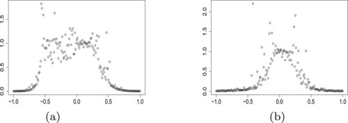
We obtained the results consistent with Theorem 4.3 from the simulations above.

1. When the coefficients of $x_1,x_2,\dots ,x_{d-1}$ approach zero, most $M^r$s are close to real number 1 that is loss reserving by IIM almost has the same accuracy as that by IDM.

2. When those coefficients are away from zero, $M^r$ tends to be zero that is the prediction accuracy of loss reserving by IIM is greatly improved with respect to IDM.

5.2. Real data analysis

In this section, we analysed a dataset, which was collected by a commercial insurance company in China. The dataset recorded writing and expiring dates of policies, individual information, see Table 1, and developments of reported claims between 1/1/2019 and 8/31/2019.

Table 1. The individual information in real data analysis.

Covariate	Description	Type	Levels
$x_1$	Insured's age	Quantitative
$x_2$	Insured's gender	Binary	female: 1, male: 0
$x_3$	Policy type	Binary	general health insurance: 1
			serious illness insurance: 0
$x_4-x_8$	Geographical location	Categorical	regions I-V: one-hot encoding with
			$(x_4,x_5,\dots ,x_8)$ so that
			region VI: $x_4=\cdots =x_8=0$

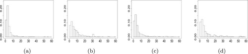
To visualise the effects of individual information on the developments of claims, for example, the histograms of reporting and settlement delays measured in days were provided under a few combinations of covariate values including gender, geographical location and age, as presented in Figures 2 and 3. It was strongly proposed that the individual information had impacts on the distributions of reporting and settlement delays.In the dataset, all the reporting delays were not more than 150 days (5 months). By China Banking and Insurance Regulatory Commission, the reported claims in health insurance are generally required to be settled within 2 months if no disagreement exists. It is appropriate to take 1 month as the time unit (‘accident year’ in previous sections). Thus the maximum reporting and settlement delays were safely set to $D^r=5$ and $D^s=3$ (the real data supported this assumption).

Figure 2. Histograms of reporting delays (in days): (a) Female, Region III, age 9–20; (b) Male, Region I, age 45–50; (c) Male, Region VI, age 20–40; (d) Male, Region III, age >55.

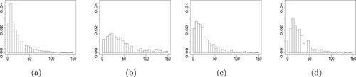
Figure 3. Histograms of settlement delays (in days): (a) Female, Region III, age 9–20; (b) Male, Region I, age 45–50; (c) Male, Region VI, age 20–40; (d) Male, Region III, age >55.

To illustrate the proposed model for loss reserving, evaluation date was set as 8/31/2019. That is, we worked with n = 8, $D^r=5$ and $D^s=3$ (months). There are four factors organised into eight features $x_1,\dots ,x_8$, as shown in Table 1. Besides, reporting and settlement delays, which were regarded as factors to model claim payments as Assumption 3.2 formulated, were respectively organised into five features $x_9$, $x_{10},\dots ,x_{13}$ and three features $x_{14},x_{15},x_{16}$.

The estimated parameters for the reporting developments under IIM, their standard errors and p-values of significance test were displayed in Table 2, while the corresponding estimated results under IDM, i.e., ${\hat{\lambda }}_u$, $u=0,1,\dots ,5$ in (7(7) $\begin{array}{r}{\hat{\lambda }}_u=\frac{{\tilde{N}}_u^r}{r_{\left(u\right)}},u=0,1,\dots ,D^r,\end{array}$(7) ) are $\begin{array}{r}(0.0218,0.0341,0.0133,0.0058,0.0034,0.0022),\end{array}$respectively. Besides, the estimated dispersion parameter $\hat{\varphi }=1.9433$. These results in (2) provide obvious evidence that individual information has effects on the reporting developments of claims in sense that most covariates associated with individual information are significant at significance level 0.05.

Similar results for settlement developments and payments are listed in Tables 3 and 4. These results also provide obvious evidence that individual information has effects on settlement developments and payments of claims. Besides, the estimated dispersion parameter ${\hat{\varphi }}^p=15467.1$ and the estimates under IDM are $\begin{array}{rl}& ({\hat{q}}_0,{\hat{q}}_1,{\hat{q}}_2,{\hat{q}}_3)=(0.6435,0.3121,0.0363,0.0081),\\ & {\hat{\mathit{\gamma }}}^{ID}=(8.3055,0.4535,0.5830,0.6227,0.58380.4557,\\ & 0.4204,0.6139,0.8472{)}^{\prime }.\end{array}$

Table 2. Estimated parameters for reporting developments, their standard errors and p-values.

	$\text{β}$			${\mathit{\pi }}_1$
	Estimate	Std. error	p-value	Estimate	Std. error	p-value
Intercept	−4.6083	0.0078	0.0000	0.8135	0.0158	0.0000
$x_1$	0.0307	0.0001	0.0000	0.0044	0.0003	0.0000
$x_2$	0.0979	0.0109	0.0000	−0.0359	0.0221	0.1044
$x_3$	1.2725	0.0114	0.0000	−0.1032	0.0231	0.0000
$x_4$	0.7215	0.0233	0.0000	−0.0277	0.0466	0.5523
$x_5$	0.6734	0.0327	0.0000	−0.1187	0.0654	0.0697
$x_6$	0.5786	0.0121	0.0000	−0.6239	0.0244	0.0000
$x_7$	0.3889	0.0145	0.0000	−0.5281	0.0292	0.0000
$x_8$	0.3114	0.3114	0.0000	−0.3829	0.0532	0.0000
	${\mathit{\pi }}_2$			${\mathit{\pi }}_3$
Intercept	−0.0198	0.0224	0.3762	−0.8734	0.0358	0.0000
$x_1$	0.0050	0.0005	0.0000	0.0064	0.0008	0.0000
$x_2$	−0.0200	0.0314	0.5239	−0.0716	0.0507	0.1575
$x_3$	0.0011	0.0322	0.9712	−0.0313	0.0515	0.5433
$x_4$	0.0685	0.0581	0.2385	0.0542	0.0917	0.5541
$x_5$	−0.1122	0.0831	0.1769	−0.4597	0.1543	0.0028
$x_6$	−0.8899	0.0361	0.0000	−0.7543	0.0549	0.0000
$x_7$	−0.8522	0.0436	0.0000	−0.8407	0.0703	0.0000
$x_8$	−0.5350	0.0734	0.0000	−0.7509	0.1305	0.0000
	${\mathit{\pi }}_4$			${\mathit{\pi }}_5$
Intercept	−1.6427	0.0525	0.0000	−2.2198	0.0768	0.0000
$x_1$	0.0057	0.0012	0.0000	0.0090	0.0017	0.0000
$x_2$	−0.0404	0.0739	0.5843	0.1614	0.1028	0.1164
$x_3$	0.0716	0.0734	0.3293	0.0059	0.1096	0.9570
$x_4$	0.4313	0.1220	0.0004	0.1285	0.2004	0.5213
$x_5$	−0.5048	0.2568	0.0494	−0.1750	0.3074	0.5691
$x_6$	−0.5444	0.0801	0.0000	−0.5695	0.1152	0.0000
$x_7$	−0.7191	0.1079	0.0000	−0.8211	0.1620	0.0000
$x_8$	−0.4864	0.1865	0.0091	−0.3980	0.2528	0.1153

Table 3. Estimated parameters for settlements developments, their standard errors and p-values.

	${\mathit{\rho }}_1$			${\mathit{\rho }}_2$
	Estimate	Std. error	p-value	Estimate	Std. error	p-value
Intercept	−0.9013	0.0124	0.0000	−2.2347	0.0354	0.0000
$x_1$	0.0046	0.0002	0.0000	0.0041	0.0008	0.0000
$x_2$	−0.0307	0.0174	0.0783	−0.1307	0.0510	0.0104
$x_3$	−0.0246	0.0182	0.1765	0.4631	0.0461	0.0000
$x_4$	0.0475	0.0368	0.1971	−0.9837	0.1058	0.0000
$x_5$	0.0230	0.0511	0.6529	−1.2136	0.1596	0.0000
$x_6$	0.0414	0.0192	0.0311	−0.8547	0.0509	0.0000
$x_7$	−0.0353	0.0232	0.1281	−1.2330	0.0749	0.0000
$x_8$	0.0831	0.0412	0.0439	−1.3182	0.1414	0.0000
	${\mathit{\rho }}_3$
Intercept	−4.8241	0.0809	0.0000
$x_1$	0.0011	0.0019	0.5482
$x_2$	−0.1864	0.1202	0.1210
$x_3$	−0.3856	0.1295	0.0029
$x_4$	0.8514	0.2535	0.0007
$x_5$	−1.7351	0.9992	0.0824
$x_6$	1.0403	0.1047	0.0000
$x_7$	0.3729	0.1047	0.0222
$x_8$	−0.2783	0.4388	0.5259

Table 4. Estimated parameters $\hat{\mathit{\gamma }}$ for payments, their standard errors and p-values.

	Estimate	Std. error	p-value
Intercept	9.3727	0.0088	0.0000
$x_1$	−0.0030	0.0002	0.0000
$x_2$	−0.1756	0.0132	0.0000
$x_3$	−2.0128	0.0311	0.0000
$x_4$	−0.0642	0.0233	0.0058
$x_5$	−0.6621	0.0409	0.0000
$x_6$	−0.4123	0.0150	0.0000
$x_7$	−0.2496	0.0151	0.0000
$x_8$	−0.3536	0.0306	0.0000
$x_9$	0.2062	0.0135	0.0000
$x_{10}$	0.7433	0.0183	0.0000
$x_{11}$	0.7745	0.0311	0.0000
$x_{12}$	0.6025	0.0529	0.0000
$x_{13}$	0.2796	0.0950	0.0032
$x_{14}$	0.3586	0.0155	0.0000
$x_{15}$	0.5814	0.0461	0.0000
$x_{16}$	0.5057	0.1174	0.0000

In Table 5, the columns with names ‘IBNR’, ‘RBNS’ and ‘Loss reserving’ correspond to estimates of IBNR reserve, RBNS reserve and total loss reserve, respectively. The square roots of approximated conditional MSEPs under IIM and IDM are in the fourth column of Table 5. The rightmost column in this table showed the computed ${\hat{M}}^r$ by (28(28) $\begin{array}{r}{\hat{M}}^r=\frac{\mathrm{V}\mathrm{a}\mathrm{r}\left(R|{\mathcal{F}}^{uo}\right)\left(\hat{\mathit{\theta }}\right)+\mathrm{\nabla }{R}_m\left(\hat{\mathit{\theta }}{)}^{\prime }\widehat{\mathrm{C}\mathrm{o}\mathrm{v}}\right(\hat{\mathit{\theta }}\left)\mathrm{\nabla }{R}_m\right(\hat{\mathit{\theta }})}{\begin{array}{c}\mathrm{V}\mathrm{a}\mathrm{r}\left(R|{\mathcal{F}}^{uo}\right)\left(\hat{\mathit{\theta }}\right)+\mathrm{\nabla }{R}_m\left(\hat{\mathit{\theta }}{)}^{\prime }\widehat{\mathrm{C}\mathrm{o}\mathrm{v}}\right(\hat{\mathit{\theta }}\left)\mathrm{\nabla }{R}_m\right(\hat{\mathit{\theta }})\\ +({\hat{R}}_{II}-{\hat{R}}_{ID}{)}^2\end{array}},\end{array}$(28) ). We can see that loss reserving by IIM provides more stable prediction of outstanding liabilities than that by IDM since the former has smaller conditional MSEP and after incorporating useful individual information into loss reserving, the prediction accuracy is greatly increased by $77.63\mathrm{\%}$.

6. Conclusion

This paper explored the improvement of accuracy in predicting outstanding liabilities, which are incurred by general insurance companies, by incorporating useful individual information into modelling. The reporting developments and payments of individual claims were given weak assumptions about their first two moments and modelled under quasi-likelihood theory, while settlement delays were modelled by multinomial logistic regression. Based on the model specification, loss reserve and conditional variance of outstanding liabilities were derived, which were further used to compute loss reserving and conditional MSEP. It was theoretically proved that loss reserving incorporating useful individual information shows higher accuracy than that under IDM, where the accuracy is measured by the conditional MSEP, when portfolio size is large enough. The conclusion is also supported by the simulations and real data analysis.

Table 5. Reserving, accuracy of prediction and accuracy improvement of IIM with respect to IDM.

Model	IBNR	RBNS	Loss reserving	$\sqrt{\widehat{\mathrm{M}\mathrm{S}\mathrm{E}\mathrm{P}}}$	${\hat{M}}^r$
IIM	56393880	24858086	81251966	2784005	0.2237
IDM	58017529	28420566	86438096	5886139

While the proposed model is basically a parametric model in statistical context, some one may be concerned with the limitation that the model is subjective and thus question its robustness in practical applications. Regarding this aspect, a possible next step is to study this problem under a nonparametric framework. Especially, it is more interesting to model the dependence of claims development on individual information by machine learning (including deep learning).

Disclosure statement

No potential conflict of interest was reported by the author(s).

Additional information

Funding

This work was supported by the Natural Science Foundation of China (71771089), the Shanghai Philosophy and Social Science Foundation (2015BGL001), the National Social Science Foundation Key Program of China (17ZDA091) and China Scholarship Council (201906140045).

Notes on contributors

Zhigao Wang

Zhigao Wang is a Ph.D. candidate in Statistics at East China Normal University.

Xianyi Wu

Xianyi Wu is a professor in School of Statistics at East China Normal University.

Chunjuan Qiu

Chunjuan Qiu is an associate professor in School of Statistics at East China Normal University.

Appendix

Proof

Proof of Proposition 3.1

To derive the following gradient and Hessian matrix, we need the identities $\frac{\mathrm{\partial }{q}_v}{\mathrm{\partial }\mathit{\rho }}=q_v({\mathit{\delta }}_v-\mathit{q})\otimes \mathit{x}$, which gives that $\begin{array}{r}\frac{\mathrm{\partial }{\mathit{q}}^{\prime }}{\mathrm{\partial }\mathit{\rho }}=\left(\mathrm{d}\mathrm{i}\mathrm{a}\mathrm{g}\right(\mathit{q})-\mathit{q}{\mathit{q}}^{\prime })\otimes \mathit{x},\frac{\mathrm{\partial }\log {\mathit{q}}^{\prime }}{\mathrm{\partial }\mathit{\rho }}=({\mathbf{I}}_{D^s}-\mathit{q}{\mathbf{1}}_{D^s}^{\prime })\otimes \mathit{x}.\end{array}$ Then we have the following gradient according to formulas above, which is $\begin{array}{rl}& \mathrm{\nabla }{Q}^{ios}\left(\mathit{\rho }\right)\\ & =\left[\sum _{v=0}^{D_i^s}{N}_v^s\right({\mathit{\delta }}_v-\mathit{q}\left)+\sum _{u=0}^{D_i^r}{N}_u^{rbns}\left(\frac{(\mathbf{0},{\overline{\mathit{q}}}_{n-i-u}^{\prime }{)}^{\prime }}{{\overline{Q}}_{n-i-u}}-\mathit{q}\right)\right]\otimes \mathit{x}\\ & =[{\mathit{N}}_i^s+\sum _{u=0}^{D_i^r}\frac{N_u^{rbns}}{{\overline{Q}}_{n-i-u}}\left(\begin{array}{c}\mathbf{0}\\ {\overline{\mathit{q}}}_{n-i-u}\end{array}\right)\\ & -(\sum _{v=0}^{D_i^s}{N}_v^s+\sum _{u=0}^{D_i^r}{N}_u^{rbns})\mathit{q}]\otimes \mathit{x}.\end{array}$By some algebraic computation, it follows that $\begin{array}{rl}& \frac{{\mathrm{\partial }}^2{Q}^{ios}\left(\mathit{\rho }\right)}{\mathrm{\partial }\mathit{\rho }{\mathit{\rho }}^{\prime }}\\ & =-\left[(\sum _{v=0}^{D_i^s}{N}_v^s+\sum _{u=0}^{D_i^r}{N}_u^{rbns})\right(\mathrm{d}\mathrm{i}\mathrm{a}\mathrm{g}\left(\mathit{q}\right)-\mathit{q}{\mathit{q}}^{\prime })\\ & +\sum _{u=0}^{D_i^r}{N}_u^{rbns}\\ & \times \left(\begin{array}{cc}\mathbf{0}& \mathbf{0}\\ \mathbf{0}& \mathrm{d}\mathrm{i}\mathrm{a}\mathrm{g}\left({\overline{\mathit{q}}}_{n-i-u}\right)-{\displaystyle \frac{{\overline{\mathit{q}}}_{n-i-u}{\overline{\mathit{q}}}_{n-i-u}^{\prime }}{{\overline{Q}}_{n-i-u}}}\end{array}\right)]\otimes \mathit{x}{\mathit{x}}^{\prime }.\end{array}$Because $\sum _{v=0}^{D_i^s}{N}_v^s+\sum _{u=0}^{D_i^r}{N}_u^{rbns}$ is just the number of those reported claims incurred in accident year i, $\begin{array}{r}\mathbb{E}[\sum _{v=0}^{D_i^s}{N}_v^s+\sum _{u=0}^{D_i^r}{N}_u^{rbns}|r,\mathit{x}]=r\sum _{u=0}^{D_i^r}{\lambda }_u.\end{array}$Observe further that $N_u^{rbns}=0$ for $i\le n-D^s$ and $0\le u\le n-i-D^s.$ Therefore, (A1) $\begin{array}{rl}& \mathbb{E}[\frac{{\mathrm{\partial }}^2{Q}^{ios}\left(\mathit{\rho }\right)}{\mathrm{\partial }\mathit{\rho }{\mathit{\rho }}^{\prime }}|r,\mathit{x}]\\ & =-r\left[\sum _{u=0}^{D_i^r}{\lambda }_u\right(\mathrm{d}\mathrm{i}\mathrm{a}\mathrm{g}\left(\mathit{q}\right)-\mathit{q}{\mathit{q}}^{\prime })\\ & -\sum _{u=(n-i-D^s+1{)}_{+}}^{D_i^r}{\lambda }_u\\ & \times \left(\begin{array}{cc}\mathbf{0}& \mathbf{0}\\ \mathbf{0}& \mathrm{d}\mathrm{i}\mathrm{a}\mathrm{g}\left({\overline{\mathit{q}}}_{n-i-u}\right)-{\displaystyle \frac{{\overline{\mathit{q}}}_{n-i-u}{\overline{\mathit{q}}}_{n-i-u}^{\prime }}{{\overline{Q}}_{n-i-u}}}\end{array}\right)]\otimes \mathit{x}{\mathit{x}}^{\prime }.\end{array}$(A1)

Let v = n−i−u and note that $\begin{array}{rl}& \mathrm{d}\mathrm{i}\mathrm{a}\mathrm{g}\left(\mathit{q}\right)-\mathit{q}{\mathit{q}}^{\prime }-\left(\begin{array}{cc}\mathbf{0}& \mathbf{0}\\ \mathbf{0}& \mathrm{d}\mathrm{i}\mathrm{a}\mathrm{g}\left({\overline{\mathit{q}}}_v\right)-{\displaystyle \frac{{\overline{\mathit{q}}}_v{\overline{\mathit{q}}}_v^{\prime }}{{\overline{Q}}_v}}\end{array}\right)\\ & =\left(\begin{array}{cc}\mathrm{d}\mathrm{i}\mathrm{a}\mathrm{g}\left({\mathit{q}}_v\right)-{\mathit{q}}_v{\mathit{q}}_v^{\prime }& -{\mathit{q}}_v{\overline{\mathit{q}}}_v^{\prime }\\ -{\overline{\mathit{q}}}_v{\mathit{q}}_v^{\prime }& {\displaystyle \frac{Q_v}{{\overline{Q}}_v}}{\overline{\mathit{q}}}_v{\overline{\mathit{q}}}_v^{\prime }\end{array}\right).\end{array}$Then, Equation (A1(A1) $\begin{array}{rl}& \mathbb{E}[\frac{{\mathrm{\partial }}^2{Q}^{ios}\left(\mathit{\rho }\right)}{\mathrm{\partial }\mathit{\rho }{\mathit{\rho }}^{\prime }}|r,\mathit{x}]\\ & =-r\left[\sum _{u=0}^{D_i^r}{\lambda }_u\right(\mathrm{d}\mathrm{i}\mathrm{a}\mathrm{g}\left(\mathit{q}\right)-\mathit{q}{\mathit{q}}^{\prime })\\ & -\sum _{u=(n-i-D^s+1{)}_{+}}^{D_i^r}{\lambda }_u\\ & \times \left(\begin{array}{cc}\mathbf{0}& \mathbf{0}\\ \mathbf{0}& \mathrm{d}\mathrm{i}\mathrm{a}\mathrm{g}\left({\overline{\mathit{q}}}_{n-i-u}\right)-{\displaystyle \frac{{\overline{\mathit{q}}}_{n-i-u}{\overline{\mathit{q}}}_{n-i-u}^{\prime }}{{\overline{Q}}_{n-i-u}}}\end{array}\right)]\otimes \mathit{x}{\mathit{x}}^{\prime }.\end{array}$(A1) ) gives rise to the desired result.

Proof

Proof of Theorem 4.1

By (3(3) $\begin{array}{r}R:=\sum _{i=1}^n{R}_i^{rbns}+\sum _{i=1}^n{R}_i^{ibnr},\end{array}$(3) ), the loss reserve can be computed as $\begin{array}{r}\mathbb{E}\left(R|{\mathcal{F}}^{uo}\right)=\mathbb{E}\left[R^{rbns}|{\mathcal{F}}^{uo}\right]+\mathbb{E}\left[R^{ibnr}|{\mathcal{F}}^{uo}\right].\end{array}$According to Assumption 3.2, for a representative policy in year i, given $N_u^{rbns}$ with $n-i-D^s+1\le u\le D_i^r$, $(N_{u,n-i-u+1},\dots ,N_{u{D}^s})$ follows multinomial distribution with parameters $N_u^{rbns}$ and $\frac{1}{{\overline{Q}}_{n-i-u}}(q_{n-i-u+1},\dots ,q_{D^s})$. Then by Assumption 3.3, the RBNS loss reserve is $\begin{array}{rl}& \mathbb{E}\left[R^{rbns}|{\mathcal{F}}^{uo}\right]\\ & =\sum _{i=1}^n\sum _{k=1}^{m_i}\sum _{u=(n-i-D^s+1{)}_{+}}^{D_i^r}\mathbb{E}\left[\sum _{v=n-i-u+1}^{D^s}\sum _{l=1}^{N_{ikuv}}{Y}_{ikuvl}|{\mathcal{F}}^{uo}\right]\\ & =\sum _{i=1}^n\sum _{k=1}^{m_i}\sum _{u=(n-i-D^s+1{)}_{+}}^{D_i^r}{N}_{iku}^{rbns}\frac{\sum _{v=n-i-u+1}^{D^s}{q}_{ikv}{\mu }_{ikuv}}{{\overline{Q}}_{ik,n-i-u}}\\ & =\sum _{v=1}^{D^s}\sum _{u=0}^{D_v^r}\sum _{k=1}^{m_{n-v-u+1}}{N}_{(n-v-u+1)ku}^{rbns}{\tilde{\mu }}_{(n-v-u+1)kuv}.\end{array}$It can be easily proved that IBNR claims are independent of historical observation ${\mathcal{F}}^{uo}$ by Assumption 3.1–3.3. Hence, IBNR loss reserve is computed by $\begin{array}{rl}\mathbb{E}\left[R^{ibnr}|{\mathcal{F}}^{uo}\right]& =E\left[\sum _{i=1}^n\sum _{k=1}^{m_i}\sum _{u=n-i+1}^{D^r}\sum _{v=0}^{D^s}\sum _{l=1}^{N_{ikuv}}{Y}_{ikuvl}|{\mathcal{F}}^{uo}\right]\\ & =\sum _{i=n-D^r+1}^n\sum _{k=1}^{m_i}\sum _{u=n-i+1}^{D^r}\sum _{v=0}^{D^s}E\left[\sum _{l=1}^{N_{ikuv}}{Y}_{ikuvl}\right]\\ & =\sum _{u=1}^{D^r}\sum _{i=n-u+1}^n\sum _{k=1}^{m_i}{p}_{iku}{r}_{ik}\exp \left({\mathit{x}}_{ik}^{\prime }\text{β}\right){\tilde{\mu }}_{iku0}.\end{array}$According to independence assumptions in Assumptions 3.1–3.3, the developments of RBNS claims are independent of developments of IBNR claims, which results in the independence between $R^{rbns}$ and $R^{ibnr}$. Then the variance of R given ${\mathcal{F}}^{uo}$ is $\begin{array}{r}\mathrm{V}\mathrm{a}\mathrm{r}\left(R|{\mathcal{F}}^{uo}\right)=\mathrm{V}\mathrm{a}\mathrm{r}\left(R^{rbns}|{\mathcal{F}}^{uo}\right)+\mathrm{V}\mathrm{a}\mathrm{r}\left(R^{ibnr}|{\mathcal{F}}^{uo}\right).\end{array}$ First, for $v\ge n-i-u+1$, we compute $\begin{array}{rl}& \mathrm{V}\mathrm{a}\mathrm{r}\left(\sum _{l=1}^{N_{uv}}{Y}_{uvl}|E^o\right)\\ & =\mathrm{V}\mathrm{a}\mathrm{r}\left(\mathbb{E}[\sum _{l=1}^{N_{uv}}{Y}_{uvl}|N_{uv},E^o]\right)\\ & +\mathbb{E}\left[\mathrm{V}\mathrm{a}\mathrm{r}(\sum _{l=1}^{N_{uv}}{Y}_{uvl}|N_{uv},E^o)\right]\\ & ={\mu }_{uv}^2\mathrm{V}\mathrm{a}\mathrm{r}\left(N_{uv}|{\mathcal{F}}^o\right)+{\varphi }^p{\mu }_{uv}\mathbb{E}\left[N_{uv}|{\mathcal{F}}^o\right]\\ & =N_u^{rbns}[{\mu }_{uv}^2\frac{q_v(1-q_v)}{{\overline{Q}}_{n-i-u}^2}+{\varphi }^p{\mu }_{uv}\frac{q_v}{{\overline{Q}}_{n-i-u}}].\end{array}$For $v_1,v_2\ge n-i-u+1$, compute $\mathrm{C}\mathrm{o}\mathrm{v}(\sum _{l=1}^{N_{u{v}_1}}{Y}_{u{v}_{1}l},\sum _{l=1}^{N_{u{v}_2}}{Y}_{u{v}_{2}l}|{\mathcal{F}}^o)$ which is equal to $\begin{array}{rl}& \mathrm{C}\mathrm{o}\mathrm{v}(\mathbb{E}[\sum _{l=1}^{N_{u{v}_1}}{Y}_{u{v}_{1}l}|N_{u{v}_1},N_{u{v}_2},{\mathcal{F}}^o],\\ & \mathbb{E}[\sum _{l=1}^{N_{u{v}_2}}{Y}_{u{v}_{2}l}|N_{u{v}_1},N_{u{v}_2},{\mathcal{F}}^o])\\ & +\mathbb{E}\left[\mathrm{C}\mathrm{o}\mathrm{v}(\sum _{l=1}^{N_{u{v}_1}}{Y}_{u{v}_{1}l},\sum _{l=1}^{N_{u{v}_2}}{Y}_{u{v}_{2}l}|N_{u{v}_1},N_{u{v}_2},{\mathcal{F}}^o)\right],\end{array}$which can be computed as follows: $\begin{array}{rl}& \mathrm{C}\mathrm{o}\mathrm{v}(\sum _{l=1}^{N_{u{v}_1}}{Y}_{u{v}_{1}l},\sum _{l=1}^{N_{u{v}_2}}{Y}_{u{v}_{2}l}|{\mathcal{F}}^o)\\ & ={\mu }_{u{v}_1}{\mu }_{u{v}_2}\mathrm{C}\mathrm{o}\mathrm{v}\left(N_{u{v}_1}|{\mathcal{F}}^o\right],N_{u{v}_2}|{\mathcal{F}}^o\left]\right)\\ & =-N_u^{rbns}{\mu }_{u{v}_1}{\mu }_{u{v}_2}\frac{q_{v_1}{q}_{v_2}}{{\overline{Q}}_{n-i-u}^2}.\end{array}$Then by independence among policies and Assumptions 3.2 and 3.3, the variance of RBNS loss reserve given ${\mathcal{F}}^{uo}$ is $\begin{array}{rl}& \mathrm{V}\mathrm{a}\mathrm{r}\left(R^{rbns}|{\mathcal{F}}^{uo}\right)\\ & =\sum _{i=1}^n\sum _{k=1}^{m_i}\mathrm{V}\mathrm{a}\mathrm{r}\left(\sum _{u=(n-i-D^s+1{)}_{+}}^{D_i^r}\sum _{v=n-i-u+1}^{D^s}\sum _{l=1}^{N_{ikuv}}{Y}_{ikuvl}|{\mathcal{F}}^{uo}\right)\\ & =\sum _{i=1}^n\sum _{k=1}^{m_i}\sum _{u=(n-i-D^s+1{)}_{+}}^{D_i^r}{N}_{iku}^{rbns}(\frac{\sum _{v=n-i-u+1}^{D^s}{q}_{ikv}{\mu }_{ikuv}^2}{{\overline{Q}}_{ik,n-i-u}^2}\\ & -{\left(\frac{\sum _{v=n-i-u+1}^{D^s}{q}_{ikv}{\mu }_{ikuv}}{{\overline{Q}}_{ik,n-i-u}}\right)}^2+{\varphi }^p\frac{\sum _{v=n-i-u+1}^{D^s}{q}_{ikv}{\mu }_{ikuv}}{{\overline{Q}}_{ik,n-i-u}})\\ & =\sum _{v=1}^{D^s}\sum _{u=0}^{D_v^r}\sum _{k=1}^{m_{n-v-u+1}}{N}_{n-v-u+1,ku}^{rbns}(\frac{{\tilde{\mu }}_{n-v-u+1,kuv}^s}{{\overline{Q}}_{n-v-u+1,k,v-1}}\\ & \phantom{\frac{{\tilde{\mu }}_{n-v-u+1,kuv}^s}{{\overline{Q}}_{n-v-u+1,k,v-1}}}-{\tilde{\mu }}_{n-v-u+1,kuv}^2+{\varphi }^p{\tilde{\mu }}_{n-v-u+1,kuv}).\end{array}$Because IBNR claims are independent of historical observation ${\mathcal{F}}^{uo}$, variance of IBNR loss reserve given ${\mathcal{F}}^{uo}$ is computed by $\begin{array}{rl}& \mathrm{V}\mathrm{a}\mathrm{r}\left(R^{ibnr}|{\mathcal{F}}^{uo}\right)\\ & =\mathrm{V}\mathrm{a}\mathrm{r}\left(\sum _{i=1}^n\sum _{k=1}^{m_i}\sum _{u=n-i+1}^{D^r}\sum _{v=0}^{D^s}\sum _{l=1}^{N_{ikuv}}{Y}_{ikuvl}\right)\\ & =\sum _{i=n-D^r+1}^n\sum _{k=1}^{m_i}\sum _{u=n-i+1}^{D^r}\mathrm{V}\mathrm{a}\mathrm{r}\left(\mathbb{E}\left[\sum _{v=0}^{D^s}\sum _{l=1}^{N_{ikuv}}{Y}_{ikuvl}|N_{iku}\right]\right)\\ & +\mathbb{E}\left[\mathrm{V}\mathrm{a}\mathrm{r}\left(\sum _{v=0}^{D^s}\sum _{l=1}^{N_{ikuv}}{Y}_{ikuvl}|N_{iku}\right)\right]\\ & =\sum _{u=1}^{D^r}\sum _{i=n-u+1}^n\sum _{k=1}^{m_i}{p}_{iku}{r}_{ik}\exp \left({\mathit{x}}_{ik}^{\prime }\text{β}\right)({\tilde{\mu }}_{iku0}^s\\ & +(\varphi -1){\tilde{\mu }}_{iku0}^2+{\varphi }^p{\tilde{\mu }}_{iku0}).\end{array}$

Proof

Proof of Theorem 4.3

Expand $R_m\left(\hat{\mathit{\theta }}\right)$ about true parameters $\mathit{\theta }$ by Taylor expansion. Then we have $\begin{array}{r}\frac{1}{m}({\hat{R}}_{II}-R_m)=\frac{1}{m}\frac{\mathrm{\partial }{R}_m\left(\mathit{\theta }\right))}{\mathrm{\partial }{\mathit{\theta }}^{\prime }}(\hat{\mathit{\theta }}-\mathit{\theta })+o_p\left(\frac{\Vert \hat{\mathit{\theta }}-\mathit{\theta }\Vert }{m}\right).\end{array}$One knows that ${\dot{\mu }}_{uv}:=\frac{\mathrm{\partial }{\mu }_{uv}}{\mathrm{\partial }\mathit{\gamma }}={\mu }_{uv}{\mathit{x}}_{uv}$. Write ${\mathit{\mu }}_{uv}=({\mu }_{u,v+1},{\mu }_{u,v+2},\dots ,{\mu }_{u,D^s}{)}^{\prime }$ and ${\dot{\mathit{\mu }}}_{uv}=\frac{\mathrm{\partial }{\mathit{\mu }}_{uv}^{\prime }}{\mathrm{\partial }\mathit{\gamma }}$, $u=0,1,\dots ,D^r$ and $v=0,\dots ,D^s-1$. To compute the partial derivative in the Taylor expansion above, we need the following partial derivatives: $\begin{array}{rl}& \frac{\mathrm{\partial }[p_{u}r\exp ({\mathit{x}}^{\prime }\text{β}\left)\right]}{\mathrm{\partial }({\text{β}}^{\prime },{\mathit{\pi }}^{\prime }{)}^{\prime }}=\left(\begin{array}{c}1\\ {\mathit{\delta }}_u-\mathit{p}\end{array}\right)\otimes (p_{u}r\exp ({\mathit{x}}^{\prime }\text{β}\left)\mathit{x}\right),\\ & \frac{\mathrm{\partial }{\tilde{\mu }}_{uv}}{\mathrm{\partial }\mathit{\rho }}=[\mathbf{0},{\mathit{\mu }}_{u,v-1}^{\prime }\left(\phantom{\frac{1}{{\overline{Q}}_{v-1}^2}}\frac{1}{{\overline{Q}}_{v-1}}\mathrm{d}\mathrm{i}\mathrm{a}\mathrm{g}\right({\overline{\mathit{q}}}_{v-1})\\ & -{\frac{1}{{\overline{Q}}_{v-1}^2}{\overline{\mathit{q}}}_{v-1}{\overline{\mathit{q}}}_{v-1}^{\prime })]}^{\prime }\otimes {\mathit{x}}_u,v\ge 1,\\ & \frac{\mathrm{\partial }{\tilde{\mu }}_{u0}}{\mathrm{\partial }\mathit{\rho }}=\left[\right(\mathrm{d}\mathrm{i}\mathrm{a}\mathrm{g}\left(\mathit{q}\right)-\mathit{q}{\mathit{q}}^{\prime }){\mathit{\mu }}_{u0}-q_0{\mu }_{u0}\mathit{q}]\otimes \mathit{x},\text{and }\\ & \frac{\mathrm{\partial }{\tilde{\mu }}_{uv}}{\mathrm{\partial }\mathit{\gamma }}=\frac{1}{{\overline{Q}}_{v-1}}\frac{\mathrm{\partial }{\mathit{\mu }}_{u,v-1}^{\prime }}{\mathrm{\partial }\mathit{\gamma }}{\overline{\mathit{q}}}_{v-1},v\ge 1,\\ & \frac{\mathrm{\partial }{\tilde{\mu }}_{u0}}{\mathrm{\partial }\mathit{\gamma }}=(\frac{\mathrm{\partial }{\mu }_{u0}}{\mathrm{\partial }\mathit{\gamma }},\frac{\mathrm{\partial }{\mathit{\mu }}_{u0}^{\prime }}{\mathrm{\partial }\mathit{\gamma }})(q_0,{\mathit{q}}^{\prime }{)}^{\prime }.\end{array}$By the law of large numbers, it can be proved that $\frac{1}{m}\frac{\mathrm{\partial }{R}_m\left(\mathit{\theta }\right))}{\mathrm{\partial }{\mathit{\theta }}^{\prime }}\stackrel{\mathrm{a}.\mathrm{s}.}{\to }\mathit{g}$, where $\mathit{g}=({\mathit{g}}_1^{\prime },{\mathit{g}}_2^{\prime },{\mathit{g}}_3^{\prime }{)}^{\prime }$, where denoting $\begin{array}{r}{M}_{uv}=\{\begin{array}{ll}{(\mathbf{0},{\mathit{\mu }}_{uv}^{\prime }\left(\mathrm{d}\mathrm{i}\mathrm{a}\mathrm{g}\right({\overline{\mathit{q}}}_v)-{\displaystyle \frac{1}{{\overline{Q}}_v}}{\overline{\mathit{q}}}_v{\overline{\mathit{q}}}_v^{\prime }))}^{\prime },& v>0\\ \left(\mathrm{d}\mathrm{i}\mathrm{a}\mathrm{g}\right({\overline{\mathit{q}}}_0)-{\displaystyle \frac{1}{{\overline{Q}}_0}}{\overline{\mathit{q}}}_0{\overline{\mathit{q}}}_0^{\prime }){\mathit{\mu }}_{u0},& v=0,\end{array}\end{array}$ (A2) $\begin{array}{rl}{\mathit{g}}_1& =\sum _{u=1}^{D^r}\sum _{i=n-u+1}^n{\kappa }_i\mathbb{E}[{\tilde{\mu }}_{u0}\left(\begin{array}{c}1\\ {\mathit{\delta }}_u-\mathit{p}\end{array}\right)\otimes (r{\lambda }_u\mathit{x}\left)\right],\\ {\mathit{g}}_2& =\sum _{u=0}^{D^r}\mathbb{E}[(\sum _{v=0}^{D^s-1}{\kappa }_{n-u-v}{M}_{uv}+\sum _{i=n-u+1}^n{\kappa }_i\\ & \times \left[\right(\mathrm{d}\mathrm{i}\mathrm{a}\mathrm{g}\left(\mathit{q}\right)-\mathit{q}{\mathit{q}}^{\prime }){\mathit{\mu }}_{u0}-q_0{\mu }_{u0}\mathit{q}]\phantom{\sum _{v=0}^{D^s-1}})\otimes \left(r{\lambda }_u\mathit{x}\right)],\\ {\mathit{g}}_3& =\sum _{u=0}^{D^r}\mathbb{E}[(\sum _{v=0}^{D^s-1}{\kappa }_{n-u-v}{\dot{\mathit{\mu }}}_{uv}{\overline{\mathit{q}}}_v\\ & +\sum _{i=n-u+1}^n{\kappa }_i({\dot{\mu }}_{u0},{\dot{\mathit{\mu }}}_{u0})(q_0,{\mathit{q}}^{\prime }{)}^{\prime }\phantom{\sum _{v=0}^{D^s-1}})\otimes \left(r{\lambda }_u{\mathit{x}}_{uv}\right)].\end{array}$(A2)

It is well known that $\hat{\mathit{\theta }}\stackrel{P}{\to }\mathit{\theta }$ under some regular conditions and hence $\frac{1}{m}({\hat{R}}_{II}-R_m)\stackrel{P}{\to }0$. Besides, $\begin{array}{rl}& \frac{\mathrm{V}\mathrm{a}\mathrm{r}\left(R|{\mathcal{F}}^{uo}\right)}{m}\stackrel{\mathrm{a}.\mathrm{s}.}{\to }{V}_R\\ & =\sum _{v=1}^{D^s}\sum _{u=0}^{D_v^r}{\kappa }_{n-v-u+1}\\ & \times \mathbb{E}\left[r{\lambda }_u{\overline{Q}}_{v-1}(\frac{{\tilde{\mu }}_{uv}^s}{{\overline{Q}}_{v-1}}-{\tilde{\mu }}_{uv}^2+{\varphi }^p{\tilde{\mu }}_{uv})\right]\\ & +\sum _{u=1}^{D^r}\sum _{i=n-u+1}^n{\kappa }_i\mathbb{E}\left[r{\lambda }_u\right({\tilde{\mu }}_{u0}^s+(\varphi -1){\tilde{\mu }}_{u0}^2+{\varphi }^p{\tilde{\mu }}_{u0}\left)\right].\end{array}$If individual data model hold true, one can similarly prove that $\frac{1}{m}({\hat{R}}_{ID}-R_m)\stackrel{P}{\to }0$. Therefore, $M^r\stackrel{P}{\to }1$ in this case. If individual information model holds true, we can easily prove that $\frac{{\hat{R}}_{ID}-R_m}{m}$ is asymptotically biased, which results from the following arguments. The law of large numbers readily gives ${\hat{h}}_v\stackrel{\mathrm{a}.\mathrm{s}.}{\to }{\check{h}}_v$ and ${\hat{\mu }}_{uv}\stackrel{\mathrm{a}.\mathrm{s}.}{\to }{\check{\mu }}_{uv}$. Further, we have ${\hat{q}}_v\stackrel{\mathrm{a}.\mathrm{s}.}{\to }{\check{q}}_v:={\check{h}}_v\prod _{s=0}^{v-1}(1-{\check{h}}_s)$ and ${\widehat{\stackrel{~}{\mu }}}_{uv}\stackrel{\mathrm{a}.\mathrm{s}.}{\to }{\check{\stackrel{~}{\mu }}}_{uv}:=\sum _{s=v}^{D^s}{\check{q}}_s{\check{\mu }}_{us}/\sum _{s=v}^{D^s}{\check{q}}_s$. We have $\begin{array}{r}\frac{{\hat{R}}_{ID}-R_m}{m}=\frac{{\hat{R}}_{ID}-{\check{R}}_{ID}}{m}+\frac{{\check{R}}_{ID}-R_m}{m},\end{array}$ where ${\check{R}}_{ID}=\sum _{v=1}^{D^s}\sum _{u=0}^{D_v^r}\sum _{k=1}^{m_{n-u-v+1}}{N}_{n-u-v+1,ku}^{rbns}{\check{\stackrel{~}{\mu }}}_{uv}+\sum _{u=1}^{D^r}\sum _{i=n-u+1}^n\sum _{k=1}^{m_i}{r}_{ik}{\check{\lambda }}_u{\check{\stackrel{~}{\mu }}}_{u0}$ and then $\begin{array}{rl}& {\check{R}}_{ID}-R_m\\ & =\sum _{v=1}^{D^s}\sum _{u=0}^{D_v^r}\sum _{k=1}^{m_{n-u-v+1}}{N}_{n-u-v+1,ku}^{rbns}({\check{\stackrel{~}{\mu }}}_{uv}-{\tilde{\mu }}_{n-u-v+1,kuv})\\ & +\sum _{u=1}^{D^r}\sum _{i=n-u+1}^n\sum _{k=1}^{m_i}(r_{ik}{\check{\lambda }}_u{\check{\stackrel{~}{\mu }}}_{u0}-r_{ik}{\lambda }_{iku}{\tilde{\mu }}_{iku0}).\end{array}$Apparently, $\frac{{\hat{R}}_{ID}-{\check{R}}_{ID}}{m}\stackrel{\mathrm{a}.\mathrm{s}.}{\to }0$ and by the law of large numbers and some simple algebra operations, we show that $\begin{array}{rl}& \frac{1}{m}({\check{R}}_{ID}-R_m)\stackrel{\mathrm{a}.\mathrm{s}.}{\to }\mathrm{\Delta }\\ & =\sum _{v=1}^{D^s}\sum _{u=0}^{D_v^r}{\kappa }_{n-v-u+1}\mathbb{E}\left[r{\lambda }_u{\overline{Q}}_{v-1}\right({\check{\stackrel{~}{\mu }}}_{uv}-{\tilde{\mu }}_{uv}\left)\right]\\ & +\sum _{u=1}^{D^r}\sum _{i=n-u+1}^n{\kappa }_i\mathbb{E}\left[r{\lambda }_u\right({\check{\stackrel{~}{\mu }}}_{u0}-{\tilde{\mu }}_{u0}\left)\right].\end{array}$Therefore, if asymptotic bias Δ is not zero, $M^r\stackrel{P}{\to }0$. Then we complete the proof.

References

- Alai, D. H., Merz, M., & Wüthrich, M. V. (2009). Mean square error of prediction in the Bornhuetter–Ferguson claims reserving method. Annals of Actuarial Science, 4(1), 7–31. https://doi.org/https://doi.org/10.1017/S1748499500000580
- Alai, D. H., Merz, M., & Wüthrich, M. V. (2010). Prediction uncertainty in the Bornhuetter–Ferguson claims reserving method: Revisited. Annals of Actuarial Science, 5(1), 7–7. https://doi.org/https://doi.org/10.1017/S1748499510000023
- Antonio, K., & Plat, R. (2014). Micro-level stochastic loss reserving for general insurance. Scandinavian Actuarial Journal, 2014(7), 649–669. https://doi.org/https://doi.org/10.1080/03461238.2012.755938
- Arjas, E. (1989). The claims reserving problem in non-life insurance: Some structural ideas. ASTIN Bulletin: The Journal of the IAA, 19(2), 139–152. https://doi.org/https://doi.org/10.2143/AST.19.2.2014905
- Crevecoeur, J., Antonio, K., & Verbelen, R. (2019). Modeling the number of hidden events subject to observation delay. European Journal of Operational Research, 277(3), 930–944. https://doi.org/https://doi.org/10.1016/j.ejor.2019.02.044
- England, P. D., & Verrall, R. J. (2002). Stochastic claims reserving in general insurance. British Actuarial Journal, 8(3), 443–544. https://doi.org/https://doi.org/10.1017/S1357321700003809
- Huang, J., Qiu, C., & Wu, X. (2015). Stochastic loss reserving in discrete time: Individual vs. aggregate data models. Communications in Statistics-Theory and Methods, 44(10), 2180–2206. https://doi.org/https://doi.org/10.1080/03610926.2014.976473
- Huang, J., Qiu, C., Wu, X., & Zhou, X. (2015). An individual loss reserving model with independent reporting and settlement. Insurance: Mathematics and Economics, 64(1), 232–245. https://doi.org/https://doi.org/10.1016/j.insmatheco.2015.05.010
- Huang, J., Wu, X., & Zhou, X. (2016). Asymptotic behaviors of stochastic reserving: Aggregate versus individual models. European Journal of Operational Research, 249(2), 657–666. https://doi.org/https://doi.org/10.1016/j.ejor.2015.09.039
- Lindholm, M., Lindskog, F., & Wahl, F. (2020). Estimation of conditional mean squared error of prediction for claims reserving. Annals of Actuarial Science, 14(1), 93–128. https://doi.org/https://doi.org/10.1017/S174849951900006X
- Mack, T. (1993). Distribution-free calculation of the standard error of chain ladder reserve estimates. ASTIN Bulletin: The Journal of the IAA, 23(2), 213–225. https://doi.org/https://doi.org/10.2143/AST.23.2.2005092
- Mack, T. (2000). Credible claims reserves: The Benktander method. ASTIN Bulletin: The Journal of the IAA, 30(2), 333–347. https://doi.org/https://doi.org/10.2143/AST.30.2.504639
- McCullagh, P., & Nelder, J. A. (1989). Generalized linear models (2nd ed). Chapman and Hall.
- Norberg, R. (1993). Prediction of outstanding liabilities in non-life insurance 1. ASTIN Bulletin: The Journal of the IAA, 23(1), 95–115. https://doi.org/https://doi.org/10.2143/AST.23.1.2005103
- Norberg, R. (1999). Prediction of outstanding liabilities II. Model variations and extensions. ASTIN Bulletin: The Journal of the IAA, 29(1), 5–25. https://doi.org/https://doi.org/10.2143/AST.29.1.504603
- Pigeon, M., Antonio, K., & Denuit, M. (2013). Individual loss reserving with the multivariate skew normal framework. ASTIN Bulletin: The Journal of the IAA, 43(3), 399–428. https://doi.org/https://doi.org/10.1017/asb.2013.20
- Pigeon, M., Antonio, K., & Denuit, M. (2014). Individual loss reserving using paid-incurred data. Insurance: Mathematics and Economics, 58(2), 121–131. https://doi.org/https://doi.org/10.1016/j.insmatheco.2014.06.012
- Van der Vaart, A. W. (2000). Asymptotic Statistics. Cambridge University Press.
- Verrall, R. J., Nielsen, J. P., & Jessen, A. H. (2010). Prediction of RBNS and IBNR claims using claim amounts and claim counts. Astin Bulletin, 40(2), 871–887. https://doi.org/https://doi.org/10.2143/AST.40.2.2061139
- Wahl, F. (2019). Explicit moments for a class of micro-models in non-life insurance. Insurance: Mathematics and Economics, 89(7), 140–156. https://doi.org/https://doi.org/10.1016/j.insmatheco.2019.10.001
- Wahl, F., Lindholm, M., & Verrall, R. (2019). The collective reserving model. Insurance: Mathematics and Economics, 87(7), 34–50. https://doi.org/https://doi.org/10.1016/j.insmatheco.2019.04.003
- Wüthrich, M. V., & Merz, M. (2008). Stochastic Claims Reserving Methods in Insurance. John Wiley and Sons.
- Yu, X., & He, R. (2016). Individual claims reserving models based on marked Cox processes. Chinese Journal of Applied Probability and Statistics 32(2), 201-219. http://aps.ecnu.edu.cn/EN/Y2016/V32/I2/201
- Zhao, X., & Zhou, X. (2010). Applying copula models to individual claim loss reserving methods. Insurance: Mathematics and Economics, 46(2), 290–299. https://doi.org/https://doi.org/10.1016/j.insmatheco.2009.11.001