Sample size and power analysis for stepped wedge cluster randomised trials with binary outcomes

Abstract

In stepped wedge cluster randomised trials (SW-CRTs), clusters of subjects are randomly assigned to sequences, where they receive a specific order of treatments. Compared to conventional cluster randomised studies, one unique feature of SW-CRTs is that all clusters start from control and gradually transition to intervention according to the randomly assigned sequences. This feature mitigates the ethical concern of withholding an effective treatment and reduces the logistic burden of implementing the intervention at multiple clusters simultaneously. This feature, however, presents challenges that need to be addressed in experimental design and data analysis, i.e., missing data due to prolonged follow-up and complicated correlation structures that involve between-subject and longitudinal correlations. In this study, based on the generalised estimating equation (GEE) approach, we present a closed-form sample size formula for SW-CRTs with a binary outcome, which offers great flexibility to account for unbalanced randomisation, missing data, and arbitrary correlation structures. We also present a correction approach to address the issue of under-estimated variance by GEE estimator when the sample size is small. Simulation studies and application to a real clinical trial are presented.

Keywords:

• Stepped wedge
• GEE
• clinical trials
• power analysis
• sample size

1. Introduction

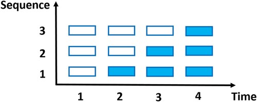
Recently, stepped wedge cluster randomised trials (SW-CRTs) are gaining popularity in large-scale biomedical and healthcare studies (Bacchieri et al., 2010; Bailet et al., 2009; Lenguerrand et al., 2020; Scalia et al., 2019; van Holland et al., 2012). Clusters of subjects are randomly assigned to different treatment sequences. Within each sequence, all clusters receive the control initially, but switch to the intervention at a particular step, as illustrated in Figure 1. There are two main types of SW-CRTs. One is the closed-cohort SW-CRT, which follows the same cohort of subjects through the treatment sequences. i.e., each subject contributes a set of longitudinal measurements. The other is the cross-sectional SW-CRT, which enrols a new panel of subjects at each step, i.e., each subject only contributes one measurement (Beard et al., 2015; Copas et al., 2015; Martin et al., 2016). SW-CRTs are considered advantageous in that (1) all clusters eventually receive the intervention, mitigating the ethical concern of withholding the effective intervention; (2) clusters switch from control to intervention in one direction only, which is more convenient in terms of washout compared to crossover studies with multiple periods; (3) they reduce the logistic burden of implementing the intervention simultaneously at many centres or facilities (Edwards, 2013; Zhou et al., 2020).

Figure 1. A diagram of an SW-CRT with 4 time points and 3 sequences (shaded and blank cells represent intervention and control, respectively.)

At the design stage, it is important to determine the number of clusters to ensure that clinical trials are adequately powered to detect effective interventions. Hussey and Hughes (2007) proposed a sample size estimation approach based on mixed-effect models for cross-sectional SW-CRTs with continuous outcomes, which also extends to binary outcomes. This approach assumes the correlation between any pairs of measurements from the same cluster to be identical, regardless of whether they are observed during the same period or not. This assumption might over-simplify reality because the correlation between concurrent observations is likely stronger than that between non-concurrent ones. Furthermore, among non-concurrent observations, the correlation might decay as observations become temporally further apart. Hooper et al. (2016) derived a sample size formula based on multilevel models for closed-cohort and cross-sectional SW-CRTs with continuous outcomes. Within clusters, a separate exchangeable correlation is assumed for concurrent and non-concurrent observations, with the former stronger than the latter. Kasza et al. (2019) proposed a sample size method that allows the correlation between non-concurrent observations to decay exponentially. Li et al. (2018) proposed sample size procedures for closed-cohort SW-CRTs with continuous and binary responses under the framework of generalised estimating equations (GEE), which employs a block exchangeable within-cluster correlation structure and this procedure can be extended to cross-sectional SW-CRTs. Zhou et al. (2020) developed a numerical power analysis method for SW-CRTs with binary outcomes based on the maximum-likelihood approach. Other developments in sample size calculation for SW-CRTs include, but are not limited to, Hemming et al. (2015), Woertman et al. (2013), Moulton et al. (2007), and Baio et al. (2015).

Most of the existing sample size methods assume relatively simpler correlation structures and no missing data, which might not hold in real SW-CRTs. Especially in closed-cohort SW-CRTs, with prolonged follow-up, the correlation structures that simultaneously involve between-subject and within-subject (longitudinal) correlations can be complicated and the problem of missing data cannot be ignored. In this study, based on the GEE approach (Liang & Zeger, 1986), we present a closed-form sample size formula for SW-CRTs with a binary outcome. It is generally applicable to both cross-sectional and closed-cohort SW-CRTs. It also provides great flexibility to account for design issues frequently encountered by practitioners including unbalanced randomisation, different severity and patterns of missing data, and complicated correlation structures.

This article is organised as follows. In Section 2, we describe the model and derive a closed-form formula to calculate the required number of clusters in SW-CRTs with binary outcomes. In Section 3, we conduct extensive simulations to evaluate the performance of the proposed method and to explore the impact of different design parameters on sample size requirement. In Section 4, we apply this method to the design of a postoperative delirium study. In Section 5, we conclude with a discussion.

2. Method

Suppose in a closed-cohort SW-CRT with T time points, n clusters are randomly assigned to S sequences (S = T−1). These clusters are randomly assigned to the sth sequence with probability $p_s$ ($s=1,\dots ,S$), where $\sum _{s=1}^S{p}_s=1$. The resulting number of clusters assigned to the sth sequence is denoted by $n_s$, with $\sum _{s=1}^S{n}_s=n$. The cluster size (number of subjects per cluster) is denoted by J. Let $Y_{sijt}$ denote the binary measurement obtained from the jth subject ($j=1,\dots ,J$) within the ith cluster ($i=1,\dots ,n_s$) under the sth sequence ($s=1,\dots ,S$) at time t ($t=1,\dots ,T)$. We define $E(Y_{sijt})={\mu }_{st}$ and ${\mu }_{st}$ is modelled by $\log \left(\frac{{\mu }_{st}}{1-{\mu }_{st}}\right)={\lambda }_t+v_{st}\zeta .$Here ${\lambda }_t$ is the time-specific intercept, $v_{st}$ is the treatment indicator with 0/1 indicating control/intervention, and ζ represents the intervention effect, which is assumed to be constant over time. The specification of ${\lambda }_t$ ($t=1,\dots ,T$) allows us to account for temporal trends of arbitrary shapes. As for the second moment, first we have $\text{Var}(Y_{sijt})={\mu }_{st}(1-{\mu }_{st})$. For the vector of longitudinal observations from each individual, ${\mathit{Y}}_{sij}=(Y_{sij1},\dots ,Y_{sijT}{)}^{\prime }$, we define $\mathbf{\Omega }=\text{Corr}({\mathit{Y}}_{sij})$ to be the within-subject (longitudinal) correlation matrix with diagonal elements ${\omega }_{tt}=1$ ($t=1,\dots ,T$). Furthermore, we use $\mathbf{\Phi }=\text{Corr}({\mathit{Y}}_{sij},{\mathit{Y}}_{si{j}^{\prime }})$ to denote correlation between subjects from the same clusters. It can be considered as the matrix version of ICC (intracluster correlation coefficient). Define ${\mathit{Y}}_{si}=({\mathit{Y}}_{si1}^{\prime },\dots ,{\mathit{Y}}_{siJ}^{\prime }{)}^{\prime }$ to be the collection of measurements from the $(s,i)$th cluster. The correlation matrix of ${\mathit{Y}}_{si}$ is $\mathit{R}={\mathit{I}}_J\otimes (\mathbf{\Omega }-\mathbf{\Phi })+\left({\mathbf{1}}_J{\mathbf{1}}_J^{\mathrm{\prime }}\right)\otimes \mathbf{\Phi },$where ⊗ is the Kronecker product operator, ${\mathit{I}}_J$ is a $J\times J$ identity matrix, and ${\mathbf{1}}_J$ is a vector of length J with all elements being 1. Finally, the observations are assumed to be independent across clusters. Hence, we complete the model specification for the first two moments of ${\mathit{Y}}_{si}$, as is required by the GEE approach (Liang & Zeger, 1986).

Define $\mathit{\beta }=({\lambda }_1,\dots ,{\lambda }_T,\zeta {)}^{\mathrm{\prime }}$ to be the vector of parameters. Based on the GEE approach with an independent working correlation structure, the estimate $\hat{\mathit{\beta }}$ can be solved from the score function $\mathit{U}(\mathit{\beta })=\mathbf{0}$ using the Newton–Raphson method, where $\mathit{U}\left(\mathit{\beta }\right)=\sum _{s=1}^S\sum _{i=1}^{n_s}\sum _{j=1}^J{\mathit{X}}_s^{\mathrm{\prime }}[{\mathit{Y}}_{sij}-{\mathit{\mu }}_s(\mathit{\beta })]$with ${\mathit{\mu }}_s=({\mu }_{s1},\dots ,{\mu }_{sT})$, and ${\mathit{X}}_s=({\mathit{I}}_T,{\mathit{v}}_s)$ is the design matrix with ${\mathit{v}}_s=(v_{s1},\dots ,v_{sT}{)}^{\prime }$. Liang and Zeger (1986) proved that as $n\to \mathrm{\infty }$, $\sqrt{n}(\hat{\mathit{\beta }}-\mathit{\beta })$ asymptotically follows a multivariate normal distribution with zero mean and covariance matrix $\mathbf{\Sigma }={\mathit{A}}^{-1}\mathit{E}{\mathit{A}}^{-1}$, where $\mathit{A}=J\sum _{s=1}^S{p}_s{\left({\mathit{X}}_s^{\mathrm{\prime }}{\mathit{G}}_s\right)}^{\otimes 2}$and $\mathit{E}=J\sum _{s=1}^S{p}_s{\mathit{X}}_s^{\mathrm{\prime }}{\mathit{G}}_s[\mathbf{\Omega }+(J-1)\mathbf{\Phi }]{\mathit{G}}_s{\mathit{X}}_s.$Here ${\mathit{G}}_s$ is a $T\times T$ diagonal matrix with the $(t,t)$th element being $\sqrt{{\mu }_{st}(1-{\mu }_{st})}$ for $t=1,\dots ,T$ and ${\mathit{C}}^{\otimes 2}={\mathit{C}\mathit{C}}^{\mathrm{\prime }}$ for a matrix $\mathit{C}$. In practice, $\mathit{A}$ and $\mathit{E}$ can be estimated by $\hat{\mathit{A}}=\frac{J}{n}\sum _{s=1}^S{n}_s{\left({\mathit{X}}_s^{\mathrm{\prime }}{\hat{\mathit{G}}}_s\right)}^{\otimes 2}$and $\hat{\mathit{E}}=n^{-1}\sum _{s=1}^S\sum _{i=1}^{n_s}{\left(\sum _{j=1}^J{\mathit{X}}_s^{\mathrm{\prime }}{\hat{\mathit{e}}}_{sij}\right)}^{\otimes 2},$where ${\hat{\mathit{e}}}_{sij}={\mathit{Y}}_{sij}-{\hat{\mathit{\mu }}}_s$ is the residual vector with ${\hat{\mathit{\mu }}}_s=({\hat{\mu }}_{s1},\dots ,{\hat{\mu }}_{sT}{)}^{\prime }$, and ${\hat{\mathit{G}}}_s$ is $T\times T$ diagonal with elements being $\sqrt{{\hat{\mu }}_{st}(1-{\hat{\mu }}_{st})}$.

Let $\hat{\zeta }$ be the estimator of ζ and ${\hat{\sigma }}_{\zeta }^2$ be the $(T+1,T+1)$th element of $\hat{\mathbf{\Sigma }}={\hat{\mathit{A}}}^{-1}\hat{\mathit{E}}{\hat{\mathit{A}}}^{-1}$. Based on the test statistic $\sqrt{n}\widehat{|\zeta |}/{\hat{\sigma }}_{\zeta }$, to reject the null hypothesis $H_0:\zeta =0$ with a power of $1-\gamma$ at a two-sided significance level of α, the required number of clusters can be computed by (1) $n=\frac{\begin{array}{c}{(z_{1-\alpha /2}+z_{1-\gamma })}^2{\displaystyle \sum _{s=1}^S{p}_s{({\mathit{v}}_s-\overline{\mathit{a}})}^{\prime }}\\ {\mathit{G}}_s[\mathbf{\Omega }+(J-1)\mathbf{\Phi }]{\mathit{G}}_s({\mathit{v}}_s-\overline{\mathit{a}})\end{array}}{{\zeta }_0^{2}J{\left[{\displaystyle \sum _{t=1}^T\left({\displaystyle \sum _{s=1}^S{w}_{st}}\right){\overline{a}}_t(1-{\overline{a}}_t)}\right]}^2},$(1) where ${\zeta }_0$ is the true intervention effect, $w_{st}=p_s{\mu }_{st}(1-{\mu }_{st})$, ${\overline{a}}_t=\frac{\sum _{s=1}^S{w}_{st}{v}_{st}}{\sum _{s=1}^S{w}_{st}}$ is the weighted proportion of subjects receiving intervention at time t, $\overline{\mathit{a}}=({\overline{a}}_1,\dots ,{\overline{a}}_T{)}^{\prime }$, and $z_c$ is the $100c$th percentile of the standard normal distribution with 0<c<1. Details of derivation are presented in Appendix .

In closed-cohort SW-CRTs, longitudinal measurements are planned on each subject at pre-specified time points. However, in real clinical trials with prolonged follow-up, the occurrence of missing data is usually inevitable. Ignoring missing data in sample size calculation will lead to under-powered studies. To address this problem, we introduce the missing indicator ${\mathrm{\Delta }}_{sijt}=0/1$ if $Y_{sijt}$ is observed/missing. We assume that the occurrence of missing data only depends on time and define the marginal observational probability $\text{Prob}({\mathrm{\Delta }}_{sijt}=1)={\delta }_t$. To accommodate different missing data patterns, we also introduce the joint observational probability $\text{Prob}({\mathrm{\Delta }}_{sijt}{\mathrm{\Delta }}_{sij{t}^{\mathrm{\prime }}}=1)={\delta }_{t{t}^{\mathrm{\prime }}}$, which is the probability that a subject contributes observations both at time t and $t^{\prime }$ ($t\ne t^{\prime }$). For example, under the independent missing (IM) pattern, the occurrences of missing data are independent between t and $t^{\prime }$, hence ${\delta }_{t{t}^{\prime }}={\delta }_t{\delta }_{t^{\prime }}$. On the other hand, under the monotone missing (MM) pattern, a subject having missing data at t would miss all subsequent observation, hence ${\delta }_{t{t}^{\prime }}={\delta }_{t^{\prime }}$ for $t^{\prime }>t$. Under the assumption of missing completely at random, $\mathit{A}$ and $\mathit{E}$ can be rewritten as ${\mathit{A}}^{\ast }=J\sum _{s=1}^S{p}_s{\mathit{X}}_s^{\mathrm{\prime }}\text{diag}\left(\mathit{\delta }\right){\mathit{G}}_s{\mathit{G}}_s{\mathit{X}}_s$and $\begin{array}{rl}{\mathit{E}}^{\ast }& =J\sum _{s=1}^S{p}_s{\mathit{X}}_s^{\mathrm{\prime }}{\mathit{G}}_s\\ & \times [\stackrel{\mathbf{~}}{\mathit{\delta }}\circ \mathbf{\Omega }+(J-1)\text{diag}\left(\mathit{\delta }\right)\mathbf{\Phi }\text{diag}\left(\mathit{\delta }\right)]{\mathit{G}}_s{\mathit{X}}_s,\end{array}$respectively. Here $\circ$ indicates the operation of Hadamard product, $\text{diag}(\mathit{\delta })$ is a $T\times T$ diagonal matrix with diagonal elements being $\mathit{\delta }=({\delta }_1,\dots ,{\delta }_T{)}^{\mathrm{\prime }}$, and $\stackrel{\mathbf{~}}{\mathit{\delta }}$ is a $T\times T$ matrix with the diagonal $(t,t)$th element being ${\delta }_t$ and off-diagonal ($t,t^{\mathrm{\prime }}$)th element being ${\delta }_{t{t}^{\mathrm{\prime }}}$. Then the generalised formula for the number of clusters accounting for missing data is (2) $n^{\ast }=\frac{\begin{array}{c}{(z_{1-\alpha /2}+z_{1-\gamma })}^2{\displaystyle \sum _{s=1}^S{p}_s{({\mathit{v}}_s-\overline{\mathit{a}})}^{\prime }{\mathit{G}}_s}\\ [\stackrel{\mathbf{~}}{\mathit{\delta }}\circ \mathbf{\Omega }+(J-1)\text{diag}\left(\mathit{\delta }\right)\mathbf{\Phi }\text{diag}\left(\mathit{\delta }\right)]{\mathit{G}}_s({\mathit{v}}_s-\overline{\mathit{a}})\end{array}}{{\zeta }_0^{2}J{\left[{\displaystyle \sum _{t=1}^T\left({\displaystyle \sum _{s=1}^S{w}_{st}}\right){\delta }_t{\overline{a}}_t(1-{\overline{a}}_t)}\right]}^2}.$(2) Formula (2(2) $n^{\ast }=\frac{\begin{array}{c}{(z_{1-\alpha /2}+z_{1-\gamma })}^2{\displaystyle \sum _{s=1}^S{p}_s{({\mathit{v}}_s-\overline{\mathit{a}})}^{\prime }{\mathit{G}}_s}\\ [\stackrel{\mathbf{~}}{\mathit{\delta }}\circ \mathbf{\Omega }+(J-1)\text{diag}\left(\mathit{\delta }\right)\mathbf{\Phi }\text{diag}\left(\mathit{\delta }\right)]{\mathit{G}}_s({\mathit{v}}_s-\overline{\mathit{a}})\end{array}}{{\zeta }_0^{2}J{\left[{\displaystyle \sum _{t=1}^T\left({\displaystyle \sum _{s=1}^S{w}_{st}}\right){\delta }_t{\overline{a}}_t(1-{\overline{a}}_t)}\right]}^2}.$(2) ) offers great flexibility to accommodate various missing data patterns (through $\stackrel{\mathbf{~}}{\mathit{\delta }},\mathit{\delta }$), complicated correlation structures (through $\mathbf{\Omega },\mathbf{\Phi }$), and unbalanced randomisation (through $p_s$). On the other hand, given n and the true treatment effect ${\zeta }_0$, the anticipated power can be evaluated by $P(Z<\sqrt{\frac{\begin{array}{c}{n}^{\ast }J{\zeta }_0^2{\displaystyle \sum _{t=1}^T\left({\displaystyle \sum _{s=1}^S{w}_{st}}\right)}\\ {\delta }_t{\overline{a}}_t(1-{\overline{a}}_t)\end{array}}{\begin{array}{c}{\displaystyle \sum _{s=1}^S{p}_s{({\mathit{v}}_s-\overline{\mathit{a}})}^{\prime }{\mathit{G}}_s}\\ [\stackrel{\mathbf{~}}{\mathit{\delta }}\circ \mathit{\Omega }+(J-1)\mathrm{diag}\\ \left(\mathit{\delta }\right)\mathbf{\Phi }\mathrm{diag}\left(\mathit{\delta }\right)]\\ {\mathit{G}}_s({\mathit{v}}_s-\overline{\mathit{a}})\end{array}}}-z_{1-\alpha /2}),$ where Z is a standard normal variable.

We have described the sample size calculation method for closed-cohort SW-CRTs with binary outcomes. In practice, many SW-CRTs are cross-sectional, where new panels of subjects are measured at each time point. Using the same notation framework, the proposed method easily accommodates cross-sectional SW-CRTs. Specifically, we consider the cluster size under a cross-sectional SW-CRT to be JT. At each time point, J subjects are selected from each cluster for measurements, and these subjects will not be selected again in the future. It implies that between-period correlation ${\omega }_{t{t}^{\prime }}$ in $\mathbf{\Omega }$ is equivalent to within-period correlation ${\varphi }_{t{t}^{\prime }}$ in $\mathbf{\Phi }$. The required number of clusters can be similarly calculated using Equation (2(2) $n^{\ast }=\frac{\begin{array}{c}{(z_{1-\alpha /2}+z_{1-\gamma })}^2{\displaystyle \sum _{s=1}^S{p}_s{({\mathit{v}}_s-\overline{\mathit{a}})}^{\prime }{\mathit{G}}_s}\\ [\stackrel{\mathbf{~}}{\mathit{\delta }}\circ \mathbf{\Omega }+(J-1)\text{diag}\left(\mathit{\delta }\right)\mathbf{\Phi }\text{diag}\left(\mathit{\delta }\right)]{\mathit{G}}_s({\mathit{v}}_s-\overline{\mathit{a}})\end{array}}{{\zeta }_0^{2}J{\left[{\displaystyle \sum _{t=1}^T\left({\displaystyle \sum _{s=1}^S{w}_{st}}\right){\delta }_t{\overline{a}}_t(1-{\overline{a}}_t)}\right]}^2}.$(2) ).

3. Simulation studies

We conducted simulation studies to evaluate the performance of the proposed sample size method. Suppose we are planning a closed-cohort SW-CRT with T = 4 time points and cluster size J = 15. We assume balanced randomisation to the S = 3 sequences, i.e., $p_1=\cdots =p_S=1/3$. We set the time-specific intercepts ${\lambda }_t=0.01(t-1)$ for $t=1,\dots ,T$. We explore two values for the intervention effect ${\zeta }_0$: 0.41 and 0.59, which corresponded to odds ratios of 1.5 and 1.8, respectively. Different correlation structures are explored: for the longitudinal correlation matrix ($\mathbf{\Omega }$), we investigate the CS and AR(1) structures, with off-diagonal elements being ${\omega }_{t{t}^{\prime }}={\rho }_1$ and ${\omega }_{t{t}^{\prime }}={\rho }_1^{|t-t^{\prime }|/(T-1)}(t\ne t^{\prime })$, respectively; for the between-subject correlation matrix, we specify $\mathbf{\Phi }=\mathbf{1}{\mathbf{1}}^{\mathbf{\prime }}{\rho }_3+({\rho }_2-{\rho }_3)\mathit{I}$ with diagonal ICC being ${\rho }_2$ and off-diagonal between-subject between-period correlation ${\rho }_3$ being 0.005. We also explored different correlation values $({\rho }_1,{\rho }_2)=\{(0.1,0.03),(0.2,0.03),(0.1,0.05),(0.2,0.05)\}$. For missing data, we considered four sets of marginal observational probabilities as follows: $\begin{array}{rl}{\mathit{\delta }}_1& =(1.00,1.00,1.00,1.00),\\ {\mathit{\delta }}_2& =(1.00,0.80,0.75,0.70),\\ {\mathit{\delta }}_3& =(1.00,0.90,0.80,0.70),\\ {\mathit{\delta }}_4& =(1.00,1.00,0.85,0.70).\end{array}$${\mathit{\delta }}_1$ represents the scenario where all subjects contribute complete observations, while ${\mathit{\delta }}_2-{\mathit{\delta }}_4$ represents scenarios of various trends in missing data, but with the same attrition rate (0.3) at the end of the study. The IM and MM missing data patterns will be explored, which leads to different joint observational probabilities (see Section 2). The null hypothesis is $H_0:\zeta =0$. We set the power $1-\gamma =0.8$ and two-sided type I error rate $\alpha =0.05$. For each combination of design parameters, we calculate the required number of clusters (n) and conducted simulations to evaluate the empirical power and type I error. The simulation algorithm is outlined as follows:

1. Calculate the required number of clusters (n) using Equation (2(2) $n^{\ast }=\frac{\begin{array}{c}{(z_{1-\alpha /2}+z_{1-\gamma })}^2{\displaystyle \sum _{s=1}^S{p}_s{({\mathit{v}}_s-\overline{\mathit{a}})}^{\prime }{\mathit{G}}_s}\\ [\stackrel{\mathbf{~}}{\mathit{\delta }}\circ \mathbf{\Omega }+(J-1)\text{diag}\left(\mathit{\delta }\right)\mathbf{\Phi }\text{diag}\left(\mathit{\delta }\right)]{\mathit{G}}_s({\mathit{v}}_s-\overline{\mathit{a}})\end{array}}{{\zeta }_0^{2}J{\left[{\displaystyle \sum _{t=1}^T\left({\displaystyle \sum _{s=1}^S{w}_{st}}\right){\delta }_t{\overline{a}}_t(1-{\overline{a}}_t)}\right]}^2}.$(2) ).

2. Generate the numbers of clusters randomised to the three sequences ($n_1,n_2,n_3$) from a multinomial distribution ($n,p_1,p_2,p_3$).

3. For each cluster, generate a vector of correlated binary measurements based on true effect $\zeta ={\zeta }_0$ and other design parameters ($\mathbf{\Omega }$ and $\mathbf{\Phi }$) based on the method of Emrich and Piedmonte (1991).

4. Generate missing indicators under different missing patterns and marginal observational probabilities $\mathit{\delta }$.

5. Calculate $\hat{\zeta }$ and ${\hat{\sigma }}_{\zeta }$. The estimation bias can be corrected using the combination of Morel et al. (2003) and Donner and Klar's (2000) methods. If $\sqrt{n}|\hat{\zeta }|/{\hat{\sigma }}_{\zeta }>z_{1-\alpha /2}$, then reject the null hypothesis.

6. Repeat Steps 2–5 5000 times. The empirical power is calculated as the proportion of iterations that reject the null hypothesis. The empirical type I error is evaluated similarly except for setting $\zeta =0$ in Step 3.

In Tables 1 and 2, the columns under ‘GEE’ present the simulation results. Each cell presents the required number of clusters as well as the empirical power and type I error. We have several observations. First, more clusters are required when longitudinal correlation (${\rho }_1$) and between-subject correlation (${\rho }_2$) get larger. For example, in the first row of Table 1, the required number of clusters changes from 45 to 46 when the longitudinal correlation (${\rho }_1$) increases from 0.1 to 0.2. On the other hand, in the first cell of Tables 1 and 2, the required number of clusters increases from 45 to 53 when the between-subject correlation (${\rho }_2$) increases from 0.03 to 0.05. Second, the longitudinal correlation structures affect the required number of clusters, which can be shown by comparing the CS and AR(1) panels in each table. Third, different missing patterns and observational probabilities affect the required number of clusters. Given the same attrition rate at the end of the study, scenarios with greater dropout initially lead to more missing data and larger sample size requirements. For example, sample sizes under ${\mathit{\delta }}_2$ are always the largest among ${\mathit{\delta }}_1$ –${\mathit{\delta }}_4$. Furthermore, under the MM missing pattern, missing data tend to concentrate on a few subjects, which leads to greater information loss and larger sample size requirement. Finally, compared with the nominal type I error of 0.05, the empirical type I errors are generally inflated (up to 0.0868). The reason is that when the number of clusters is relatively small, the conventional GEE approach tends to underestimate the variance of the treatment effect (Morel et al., 2003).

Table 1. Required number of clusters (empirical power, empirical type I error) for closed-cohort studies with ${\rho }_2=0.03$.

		Missing		GEE		Adjusted GEE
	${\zeta }_0$	Pattern	$\mathit{\delta }$	${\rho }_1=0.1$	${\rho }_1=0.2$	${\rho }_1=0.1$	${\rho }_1=0.2$
CS	log(1.5)	IM	${\mathit{\delta }}_1$	45 (0.8218, 0.0600)	46 (0.8150, 0.0630)	47 (0.7958, 0.0540)	48 (0.7994, 0.0504)
			${\mathit{\delta }}_2$	53 (0.8050, 0.0608)	55 (0.8132, 0.0606)	55 (0.7900, 0.0546)	57 (0.7966, 0.0460)
			${\mathit{\delta }}_3$	50 (0.8104, 0.0636)	51 (0.8044, 0.0592)	52 (0.7940, 0.0440)	53 (0.7862, 0.0496)
			${\mathit{\delta }}_4$	47 (0.8056, 0.0666)	48 (0.8098, 0.0598)	49 (0.7938, 0.0504)	50 (0.7874, 0.0448)
		MM	${\mathit{\delta }}_2$	53 (0.8080, 0.0602)	55 (0.7998, 0.0546)	55 (0.7914, 0.0406)	57 (0.7884, 0.0472)
			${\mathit{\delta }}_3$	50 (0.8050, 0.0624)	52 (0.8058, 0.0650)	52 (0.7970, 0.0516)	54 (0.8044, 0.0506)
			${\mathit{\delta }}_4$	47 (0.8102, 0.0608)	48 (0.8098, 0.0656)	49 (0.7978, 0.0494)	50 (0.7952, 0.0472)
	log(1.8)	IM	${\mathit{\delta }}_1$	22 (0.8152, 0.0784)	23 (0.8188, 0.0868)	24 (0.7862, 0.0484)	25 (0.7920, 0.0420)
			${\mathit{\delta }}_2$	26 (0.8154, 0.0840)	27 (0.8144, 0.0700)	28 (0.7850, 0.0454)	29 (0.7940, 0.0472)
			${\mathit{\delta }}_3$	25 (0.8256, 0.0762)	25 (0.8192, 0.0766)	27 (0.7864, 0.0454)	27 (0.7920, 0.0470)
			${\mathit{\delta }}_4$	23 (0.8092, 0.0726)	24 (0.8176, 0.0692)	25 (0.7908, 0.0474)	26 (0.7908, 0.0454)
		MM	${\mathit{\delta }}_2$	26 (0.8106, 0.0782)	27 (0.8228, 0.0754)	28 (0.7894, 0.0430)	29 (0.7954, 0.0438)
			${\mathit{\delta }}_3$	25 (0.8132, 0.0744)	25 (0.7982, 0.0782)	27 (0.7982, 0.0498)	27 (0.7862, 0.0494)
			${\mathit{\delta }}_4$	23 (0.8126, 0.0738)	24 (0.8146, 0.0742)	25 (0.7900, 0.0486)	26 (0.8008, 0.0432)
AR(1)	log(1.5)	IM	${\mathit{\delta }}_1$	50 (0.8066, 0.0598)	52 (0.8226, 0.0608)	52 (0.8100, 0.0482)	54 (0.8010, 0.0464)
			${\mathit{\delta }}_2$	58 (0.8082, 0.0600)	60 (0.8128, 0.0650)	60 (0.8020, 0.0528)	62 (0.8058, 0.0504)
			${\mathit{\delta }}_3$	55 (0.7964, 0.0626)	57 (0.7990, 0.0606)	57 (0.7934, 0.0508)	59 (0.8108, 0.0476)
			${\mathit{\delta }}_4$	52 (0.8034, 0.0650)	54 (0.7912, 0.0626)	54 (0.7858, 0.0498)	56 (0.8044, 0.0532)
		MM	${\mathit{\delta }}_2$	60 (0.8118, 0.0586)	62 (0.8124, 0.0620)	62 (0.8136, 0.0508)	64 (0.8026, 0.0502)
			${\mathit{\delta }}_3$	56 (0.8106, 0.0570)	58 (0.8116, 0.0570)	58 (0.8018, 0.0464)	60 (0.8038, 0.0526)
			${\mathit{\delta }}_4$	52 (0.8070, 0.0628)	54 (0.8110, 0.0532)	54 (0.7986, 0.0472)	56 (0.8048, 0.0528)
	log(1.8)	IM	${\mathit{\delta }}_1$	25 (0.8212, 0.0750)	25 (0.8112, 0.0738)	27 (0.8134, 0.0464)	27 (0.7930, 0.0472)
			${\mathit{\delta }}_2$	29 (0.8158, 0.0744)	30 (0.8268, 0.0714)	31 (0.8076, 0.0554)	32 (0.8086, 0.0490)
			${\mathit{\delta }}_3$	27 (0.8178, 0.0698)	28 (0.8140, 0.0710)	29 (0.7924, 0.0554)	30 (0.8032, 0.0504)
			${\mathit{\delta }}_4$	26 (0.8216, 0.0728)	27 (0.8226, 0.0780)	28 (0.7982, 0.0482)	29 (0.7984, 0.0456)
		MM	${\mathit{\delta }}_2$	30 (0.8170, 0.0746)	31 (0.8184, 0.0732)	32 (0.8102, 0.0514)	33 (0.8120, 0.0492)
			${\mathit{\delta }}_3$	27 (0.8156, 0.0780)	28 (0.8200, 0.0694)	29 (0.7944, 0.0452)	30 (0.7884, 0.0506)
			${\mathit{\delta }}_4$	26 (0.8142, 0.0750)	27 (0.8222, 0.0782)	28 (0.7866, 0.0490)	29 (0.8002, 0.0480)

Table 2. Required number of clusters (empirical power, empirical type I error) for closed-cohort studies with ${\rho }_2=0.05$.

		Missing		GEE		Adjusted GEE
	${\zeta }_0$	Pattern	$\mathit{\delta }$	${\rho }_1=0.1$	${\rho }_1=0.2$	${\rho }_1=0.1$	${\rho }_1=0.2$
CS	log(1.5)	IM	${\mathit{\delta }}_1$	53 (0.8058, 0.0584)	54 (0.7968, 0.0558)	55 (0.7912, 0.0466)	56 (0.7918, 0.0466)
			${\mathit{\delta }}_2$	61 (0.7958, 0.0634)	63 (0.8104, 0.0564)	63 (0.7926, 0.0494)	65 (0.7968, 0.0524)
			${\mathit{\delta }}_3$	58 (0.8048, 0.0628)	59 (0.8046, 0.0598)	60 (0.7908, 0.0438)	61 (0.7986, 0.0504)
			${\mathit{\delta }}_4$	55 (0.8004, 0.0620)	57 (0.8114, 0.0636)	57 (0.7946, 0.0500)	59 (0.7998, 0.0488)
		MM	${\mathit{\delta }}_2$	62 (0.8108, 0.0586)	63 (0.8084, 0.0552)	64 (0.7996, 0.0490)	65 (0.7996, 0.0486)
			${\mathit{\delta }}_3$	58 (0.8004, 0.0596)	60 (0.8062, 0.0546)	60 (0.7960, 0.0472)	62 (0.7980, 0.0520)
			${\mathit{\delta }}_4$	55 (0.7932, 0.0642)	57 (0.8172, 0.0618)	57 (0.7838, 0.0496)	59 (0.7946, 0.0516)
	log(1.8)	IM	${\mathit{\delta }}_1$	26 (0.8128, 0.0756)	27 (0.8220, 0.0692)	28 (0.7888, 0.0436)	29 (0.7994, 0.0446)
			${\mathit{\delta }}_2$	30 (0.8168, 0.0688)	31 (0.8146, 0.0750)	32 (0.7828, 0.0484)	33 (0.7916, 0.0498)
			${\mathit{\delta }}_3$	29 (0.8226, 0.0782)	29 (0.8078, 0.0752)	31 (0.7964, 0.0478)	31 (0.7818, 0.0420)
			${\mathit{\delta }}_4$	27 (0.8020, 0.0784)	28 (0.8154, 0.0728)	29 (0.7850, 0.0448)	30 (0.7918, 0.0544)
		MM	${\mathit{\delta }}_2$	30 (0.8102, 0.0682)	31 (0.8092, 0.0714)	32 (0.7902, 0.0488)	33 (0.7908, 0.0506)
			${\mathit{\delta }}_3$	29 (0.8262, 0.0706)	29 (0.8086, 0.0732)	31 (0.7970, 0.0440)	31 (0.7816, 0.0466)
			${\mathit{\delta }}_4$	27 (0.8136, 0.0694)	28 (0.8144, 0.0658)	29 (0.7878, 0.0468)	30 (0.7970, 0.0464)
AR(1)	log(1.5)	IM	${\mathit{\delta }}_1$	58 (0.8036, 0.0616)	60 (0.8056, 0.0628)	60 (0.7948, 0.0532)	62 (0.8052, 0.0492)
			${\mathit{\delta }}_2$	67 (0.8034, 0.0552)	68 (0.8092, 0.0514)	69 (0.7992, 0.0482)	70 (0.8014, 0.0464)
			${\mathit{\delta }}_3$	63 (0.8054, 0.0626)	65 (0.8148, 0.0578)	65 (0.8016, 0.0516)	67 (0.8000, 0.0508)
			${\mathit{\delta }}_4$	61 (0.8050, 0.0626)	62 (0.8030, 0.0672)	63 (0.8054, 0.0470)	64 (0.7902, 0.0490)
		MM	${\mathit{\delta }}_2$	68 (0.7986, 0.0584)	71 (0.8166, 0.0634)	70 (0.7964, 0.0484)	73 (0.8100, 0.0464)
			${\mathit{\delta }}_3$	64 (0.8026, 0.0526)	66 (0.8124, 0.0628)	66 (0.7984, 0.0438)	68 (0.8040, 0.0476)
			${\mathit{\delta }}_4$	61 (0.8168, 0.0570)	62 (0.7916, 0.0632)	63 (0.7988, 0.0446)	64 (0.7970, 0.0526)
	log(1.8)	IM	${\mathit{\delta }}_1$	29 (0.8128, 0.0710)	29 (0.8008, 0.0700)	31 (0.8066, 0.0424)	31 (0.7882, 0.0442)
			${\mathit{\delta }}_2$	33 (0.8094, 0.0736)	34 (0.8132, 0.0660)	35 (0.8006, 0.0506)	36 (0.8004, 0.0474)
			${\mathit{\delta }}_3$	31 (0.8058, 0.0658)	32 (0.8096, 0.0754)	33 (0.7878, 0.0460)	34 (0.8004, 0.0534)
			${\mathit{\delta }}_4$	30 (0.8128, 0.0722)	31 (0.8306, 0.0672)	32 (0.8044, 0.0460)	33 (0.8080, 0.0470)
		MM	${\mathit{\delta }}_2$	34 (0.8142, 0.0772)	35 (0.8156, 0.0624)	36 (0.8080, 0.0488)	37 (0.8128, 0.0520)
			${\mathit{\delta }}_3$	31 (0.8038, 0.0726)	32 (0.8184, 0.0682)	33 (0.7814, 0.0464)	34 (0.7930, 0.0526)
			${\mathit{\delta }}_4$	30 (0.8180, 0.0720)	31 (0.8286, 0.0736)	32 (0.7952, 0.0484)	33 (0.8056, 0.0506)

To address the issue of underestimated variance, we have explored different correction methods, including Mancl and DeRouen (2001), Kauermann and Carroll (2001), Ziegler and Vens (2010), Morel et al. (2003), Fay and Graubard (2001) and Pan and Wall (2002). We find that the combination of Morel et al. (2003) (MBN) and Donner and Klar's (2000) methods achieves a good balance between satisfactory performance and easy implementation in practice. Specifically, the MBN method modifies the GEE covariance estimator with an additional term $\begin{array}{rl}{\mathbf{\Sigma }}_{MBN}& ={\mathit{A}}^{-1}\mathit{E}{\mathit{A}}^{-1}+min\{0.5,\frac{T+1}{n-T-1}\}\\ & \times max\{1,\frac{1}{T+1}\text{trace}({\mathit{A}}^{-1}\mathit{E})\}{\mathit{A}}^{-1}.\end{array}$Donner and Klar's (2000) method suggests adding one cluster to each treatment arm. The results under this combination approach are presented in Tables 1 and 2 under the columns of ‘Adjusted GEE’. The empirical powers and type I errors are very close to their nominal values of 0.8 and 0.05, respectively. For example, in Table 1 when the number of clusters is less than 30, the type I errors without adjustment are all severely inflated (larger than 0.07). After adjustment, all the type I errors are close to the nominal level 0.05.

We also conduct simulations to investigate the performance of the proposed method in cross-sectional SW-CRTs. Because each subject only contributes one measurement, the issue of missing data does not apply. We set $\mathbf{\Omega }=\mathbf{1}{\mathbf{1}}^{\mathbf{\prime }}\rho +(1-\rho )\mathit{I}$ and $\mathbf{\Phi }=\mathbf{1}{\mathbf{1}}^{\mathbf{\prime }}\rho$. Two values are explored for ρ: 0.03 and 0.05. Table 3 presents the required number of clusters with empirical power and type I error for cross-sectional SW-CRTs. Similar to the observations from the closed-cohort SW-CRTs, a smaller correlation (ρ) is associated with a smaller sample size requirement. Furthermore, the proposed correction approach performs well in maintaining the empirical powers and type I errors at their nominal levels.

Table 3. Required number of clusters (empirical power, empirical type I error) for cross-sectional studies.

	GEE		Adjusted GEE
${\zeta }_0$	$\rho =0.03$	$\rho =0.05$	$\rho =0.03$	$\rho =0.05$
log(1.5)	49 (0.8077, 0.0600)	61 (0.8116, 0.0616)	51 (0.7935, 0.0495)	63 (0.7919, 0.0543)
log(1.8)	24 (0.8091, 0.0850)	30 (0.8136, 0.0781)	26 (0.7948, 0.0492)	32 (0.8001, 0.0511)

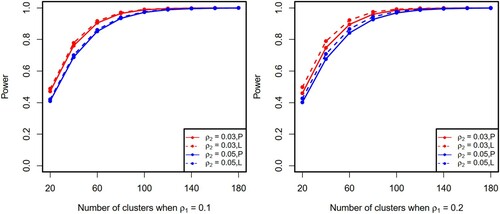
We performed additional simulations to evaluate the relationship between the required number of clusters and power. We used the same parameter settings as described above for closed-cohort studies with the CS correlation structures. Under different combinations of design parameters, as shown in Figure 2 (solid lines), testing power increases as the number of clusters increases. Furthermore, we compared the proposed method with an existing method (Li et al., 2018). Since Li's method does not account for missing data, we only consider the scenario of complete observations. To maximise the usability of the proposed sample size method in pragmatic settings, we assume that when analysing trial data researchers do not know the true correlation structure and make inference using GEE with independent working correlation. This practical solution is slightly less efficient than Li's method which uses the true correlation (see Figure 2). We believe the proposed method nonetheless provides a useful sample size solution for the design of pragmatic SW-CRTs because it compensates for a slight loss in efficiency by advantages in (1) a closed-form sample size formula; (2) accommodation of missing data; and (3) not requiring the true correlation to be known during inference.

Figure 2. Relationship between the number of clusters and power (P and L denote the proposed method and Li's method, respectively).

4. Example

We apply the proposed method to a cross-sectional SW-CRT study (Mouchoux et al., 2011), which was designed to evaluate whether a multifaceted programme (including consulting and training, etc.) could decrease postoperative delirium in patients aged 75 and older. The outcome of interest is the occurrence of delirium within seven days after surgery. Suppose this study is conducted over a six-month period with T = 4 pre-specified time points and surgical wards are assigned to S = 3 sequences with balanced randomisation. At each time point, 15 patients per surgical ward will receive assigned intervention and the delirium outcome will be recorded. It is hypothesised that the multifaceted programme can reduce the occurrence of delirium from 60% to 40%, which corresponds to an odds ratio of 0.44 and a constant time effect of 0.41. By assuming $\rho =0.05$ in $\mathbf{\Omega }=\mathbf{1}{\mathbf{1}}^{\mathbf{\prime }}\rho +(1-\rho )\mathit{I}$ and $\mathbf{\Phi }=\mathbf{1}{\mathbf{1}}^{\mathbf{\prime }}\rho$, we will need 16 wards to achieve 80% power at a two-sided significance level of 0.05. If 30 patients are selected per surgical ward for measurements, 12 wards will be needed.

5. Discussion

In this study, we propose a sample size and power calculation method that is generally applicable to both closed-cohort and cross-sectional SW-CRTs with binary outcomes. We directly incorporate several design issues encountered in pragmatic trials into power analysis and were able to provide a closed-form sample size solution. Through different specifications of correlation matrices $\mathbf{\Omega }$ and $\mathbf{\Phi }$, the proposed method offers great flexibility to account for different types of SW-CRTs and correlation structures. The inclusion of parameters $p_s$ allows researchers to employ unbalanced randomisation. Furthermore, our method maintains the desired power in the presence of missing data through the specification of marginal observational probabilities at population level ($\mathit{\delta }$), and the missing pattern at subject level ($\stackrel{\mathbf{~}}{\mathit{\delta }}$). In simulation studies, we have investigated the independent (IM) and monotone (MM) missing patterns. In practice, a clinical trial might encounter different types of missing patterns. For example, it is possible that some subjects miss a few appointments due to accidents (IM), while some subjects drop out in the middle of study (MM). The proposed sample size method can accommodate such scenarios by specifying a mixture of IM and MM, where ${\delta }_t^{\left(MIX\right)}=w{\delta }_t^{\left(IM\right)}+(1-w){\delta }_t^{\left(MM\right)}$and ${\delta }_{t{t}^{\mathrm{\prime }}}^{\left(MIX\right)}=w{\delta }_{t{t}^{\mathrm{\prime }}}^{\left(IM\right)}+(1-w){\delta }_{t{t}^{\mathrm{\prime }}}^{\left(MM\right)},$where w and 1−w are weights for IM and MM, respectively. Finally, we have present a correction approach to address the issue of underestimated variance by the GEE method when the number of clusters is limited in SW-CRTs.

Disclosure statement

No potential conflict of interest was reported by the author(s).

Additional information

Funding

This work was supported by the Patient-Centered Outcomes Research Institute [ME-1609-36761].

Appendix. Derivation of Equation (1)

First we have $\hat{\mathit{A}}=\frac{J}{n}\sum _{s=1}^S{n}_s{\left({\mathit{X}}_s^{\mathrm{\prime }}{\hat{\mathit{G}}}_s\right)}^{\otimes 2}.$As $n\to \mathrm{\infty }$, $\hat{\mathit{A}}$ approaches $\mathit{A}=J\sum _{s=1}^S{p}_s{\left({\mathit{X}}_s^{\mathrm{\prime }}{\mathit{G}}_s\right)}^{\otimes 2}$On the other hand, we have $\begin{array}{rl}\hat{\mathit{E}}& =n^{-1}\sum _{s=1}^S\sum _{i=1}^{n_s}{\left(\sum _{j=1}^J{\mathit{X}}_s^{\mathrm{\prime }}{\hat{\mathit{e}}}_{\mathit{s}\mathit{i}\mathit{j}}\right)}^{\otimes 2}\\ & =n^{-1}\sum _{s=1}^S\sum _{i=1}^{n_s}\left(\sum _{j=1}^J{\mathit{X}}_{\mathit{s}}^{\mathbf{\prime }}{\hat{\mathit{e}}}_{\mathit{s}\mathit{i}\mathit{j}}\right)\left(\sum _{j=1}^J{\hat{\mathit{e}}}_{\mathit{s}\mathit{i}\mathit{j}}^{\mathbf{\prime }}{\mathit{X}}_{\mathit{s}}\right)\\ & =n^{-1}\sum _{s=1}^S\sum _{i=1}^{n_s}\left(\sum _{j=1}^J\sum _{j^{\mathrm{\prime }}=1}^J{\mathit{X}}_{\mathit{s}}^{\mathbf{\prime }}{\hat{\mathit{e}}}_{\mathit{s}\mathit{i}\mathit{j}}{\hat{\mathit{e}}}_{\mathit{s}\mathit{i}{\mathit{j}}^{\mathbf{\prime }}}^{\mathbf{\prime }}{\mathit{X}}_{\mathit{s}}\right)\\ & =n^{-1}\sum _{s=1}^S\sum _{i=1}^{n_s}\left(\sum _{j=1}^J{\mathit{X}}_{\mathit{s}}^{\mathbf{\prime }}{\hat{\mathit{e}}}_{\mathit{s}\mathit{i}\mathit{j}}{\hat{\mathit{e}}}_{\mathit{s}\mathit{i}\mathit{j}}^{\mathbf{\prime }}{\mathit{X}}_{\mathit{s}}+2\sum _{j=1}^{J-1}\sum _{j^{\mathrm{\prime }}=j+1}^J{\mathit{X}}_{\mathit{s}}^{\mathbf{\prime }}{\hat{\mathit{e}}}_{\mathit{s}\mathit{i}\mathit{j}}{\hat{\mathit{e}}}_{\mathit{s}\mathit{i}{\mathit{j}}^{\mathbf{\prime }}}^{\mathbf{\prime }}{\mathit{X}}_{\mathit{s}}\right).\end{array}$As $n\to \mathrm{\infty }$, $\hat{\mathit{E}}$ approaches $\mathit{E}=J\sum _{s=1}^S{p}_s{\mathit{X}}_s^{\mathrm{\prime }}{\mathit{G}}_s[\mathbf{\Omega }+(J-1)\mathbf{\Phi }]{\mathit{G}}_s{\mathit{X}}_s.$We are only interested in ${\sigma }_{\zeta }^2$, which is the $(T+1,T+1)$-component of ${\mathbf{\Sigma }\mathbf{=}\mathit{A}}^{-1}\mathit{E}{\mathit{A}}^{-1}$. The last row of ${\mathit{A}}^{-1}$ can be simplified as ${[J\sum _{t=1}^T\sum _{s=1}^S{w}_{st}{\overline{a}}_t(1-{\overline{a}}_t)]}^{-1}\left[\begin{array}{cc}-\overline{\mathit{a}}& 1\end{array}\right],$where $w_{st}=p_s{\mu }_{st}(1-{\mu }_{st})$, ${\overline{a}}_t=\frac{\sum _{s=1}^S{w}_{st}{v}_{st}}{\sum _{s=1}^S{w}_{st}}$ is the weighted proportion of subjects receiving intervention at time t, and $\overline{\mathit{a}}=({\overline{a}}_1,\dots ,{\overline{a}}_T{)}^{\prime }$. Then, we have $\begin{array}{rl}{\sigma }_{\zeta }^2& ={[J\sum _{t=1}^T\sum _{s=1}^S{w}_{st}{\overline{a}}_t(1-{\overline{a}}_t)]}^{-2}\left[\begin{array}{cc}-\overline{\mathit{a}}& 1\end{array}\right]\mathit{E}{\left[\begin{array}{cc}-\overline{\mathit{a}}& 1\end{array}\right]}^{\mathrm{\prime }}\\ & ={[J\sum _{t=1}^T\sum _{s=1}^S{w}_{st}{\overline{a}}_t(1-{\overline{a}}_t)]}^{-2}\left[\begin{array}{cc}-\overline{\mathit{a}}& 1\end{array}\right]J\sum _{s=1}^S{p}_s{\mathit{X}}_s^{\mathrm{\prime }}{\mathit{G}}_s\\ & \times [\mathbf{\Omega }+(J-1)\mathbf{\Phi }]{\mathit{G}}_s{\mathit{X}}_s{\left[\begin{array}{cc}-\overline{\mathit{a}}& 1\end{array}\right]}^{\mathrm{\prime }}\\ & =\frac{{\displaystyle \sum _{s=1}^S{p}_s{({\mathit{v}}_s-\overline{\mathit{a}})}^{\prime }{\mathit{G}}_s[\mathbf{\Omega }+(J-1)\mathbf{\Phi }]{\mathit{G}}_s({\mathit{v}}_s-\overline{\mathit{a}})}}{J{\left[{\displaystyle \sum _{t=1}^T\left({\displaystyle \sum _{s=1}^S{w}_{st}}\right){\overline{a}}_t(1-{\overline{a}}_t)}\right]}^2}.\end{array}$The required number of clusters is $\begin{array}{rl}n& =\frac{{(z_{1-\alpha /2}+z_{1-\gamma })}^2{\sigma }_{\zeta }^2}{{\zeta }_0^2}\\ & =\frac{\begin{array}{c}{(z_{1-\alpha /2}+z_{1-\gamma })}^2{\displaystyle \sum _{s=1}^S{p}_s{({\mathit{v}}_s-\overline{\mathit{a}})}^{\prime }}\\ {\mathit{G}}_s[\mathbf{\Omega }+(J-1)\mathbf{\Phi }]{\mathit{G}}_s({\mathit{v}}_s-\overline{\mathit{a}})\end{array}}{{\zeta }_0^{2}J{\left[{\displaystyle \sum _{t=1}^T\left({\displaystyle \sum _{s=1}^S{w}_{st}}\right){\overline{a}}_t(1-{\overline{a}}_t)}\right]}^2}.\end{array}$

References

- Bacchieri, G., Barros, A. J., Gonçalves, H., & Gigante, D. P. (2010). A community intervention to prevent traffic accidents among bicycle commuters. Revista De Saude Publica, 44(5), 867–875. https://doi.org/10.1590/S0034-89102010000500012
- Bailet, L. L., Repper, K. K., Piasta, S. B., & Murphy, S. P. (2009). Emergent literacy intervention for prekindergarteners at risk for reading failure. Journal of Learning Disabilities, 42(4), 336–355. https://doi.org/10.1177/0022219409335218
- Baio, G., Copas, A., Ambler, G., Hargreaves, J., Beard, E., & Omar, R. Z. (2015). Sample size calculation for a stepped wedge trial. Trials, 16(1), 354. https://doi.org/10.1186/s13063-015-0840-9
- Beard, E., Lewis, J. J., Copas, A., Davey, C., Osrin, D., Baio, G., Thompson, J. A., Fielding, K. L., Omar, R. Z., Ononge, S., Hargreaves, J., & Prost, A. (2015). Stepped wedge randomised controlled trials: systematic review of studies published between 2010 and 2014. Trials, 16(1), 353. https://doi.org/10.1186/s13063-015-0839-2
- Copas, A. J., Lewis, J. J., Thompson, J. A., Davey, C., Baio, G., & Hargreaves, J. R. (2015). Designing a stepped wedge trial: three main designs, carry-over effects and randomisation approaches. Trials, 16(1), 352. https://doi.org/10.1186/s13063-015-0842-7
- Donner, A., & Klar, N. (2000). Design and analysis of cluster randomization trials in health research. Arnold.
- Edwards, S. J. (2013). Ethics of clinical science in a public health emergency: Drug discovery at the bedside. The American Journal of Bioethics, 13(9), 3–14. https://doi.org/10.1080/15265161.2013.813597
- Emrich, L. J., & Piedmonte, M. R. (1991). A method for generating high-dimensional multivariate binary variates. The American Statistician, 45(4), 302–304. https://doi.org/10.2307/2684460
- Fay, M. P., & Graubard, B. I. (2001). Small-sample adjustments for Wald-type tests using sandwich estimators. Biometrics, 57(4), 1198–1206. https://doi.org/10.1111/j.0006-341X.2001.01198.x
- Hemming, K., Haines, T. P., Chilton, P. J., Girling, A. J., & Lilford, R. J. (2015). The stepped wedge cluster randomised trial: Rationale, design, analysis, and reporting. BMJ (Clinical Research Ed.), 350, h391. https://doi.org/10.1136/bmj.h391
- Hooper, R., Teerenstra, S., de Hoop, E., & Eldridge, S. (2016). Sample size calculation for stepped wedge and other longitudinal cluster randomised trials. Statistics in Medicine, 35(26), 4718–4728. https://doi.org/10.1002/sim.v35.26
- Hussey, M. A., & Hughes, J. P. (2007). Design and analysis of stepped wedge cluster randomized trials. Contemporary Clinical Trials, 28(2), 182–191. https://doi.org/10.1016/j.cct.2006.05.007
- Kasza, J., Hemming, K., Hooper, R., Matthews, J., & Forbes, A. (2019). Impact of non-uniform correlation structure on sample size and power in multiple-period cluster randomised trials. Statistical Methods in Medical Research, 28(3), 703–716. https://doi.org/10.1177/0962280217734981
- Kauermann, G., & Carroll, R. J. (2001). A note on the efficiency of sandwich covariance matrix estimation. Journal of the American Statistical Association, 96(456), 1387–1396. https://doi.org/10.1198/016214501753382309
- Lenguerrand, E., Winter, C., Siassakos, D., MacLennan, G., Innes, K., Lynch, P., Cameron, A., Crofts, J., McDonald, A., McCormack, K., Forrest, M., Norrie, J., Bhattacharya, S., & Draycott, T. (2020). Effect of hands-on interprofessional simulation training for local emergencies in Scotland: The thistle stepped-wedge design randomised controlled trial. BMJ Quality & Safety, 29(2), 122–134. https://doi.org/10.1136/bmjqs-2018-008625
- Li, F., Turner, E. L., & Preisser, J. S. (2018). Sample size determination for GEE analyses of stepped wedge cluster randomized trials. Biometrics, 74(4), 1450–1458. https://doi.org/10.1111/biom.v74.4
- Liang, K. Y., & Zeger, S. L. (1986). Longitudinal data analysis for discrete and continuous outcomes using generalized linear models. Biometrika, 84, 3–32. https://doi.org/10.2307/2531248
- Mancl, L. A., & DeRouen, T. A. (2001). A covariance estimator for GEE with improved small-sample properties. Biometrics, 57(1), 126–134. https://doi.org/10.1111/biom.2001.57.issue-1
- Martin, J., Taljaard, M., Girling, A., & Hemming, K. (2016). Systematic review finds major deficiencies in sample size methodology and reporting for stepped-wedge cluster randomised trials. BMJ Open, 6(2), e010166. https://doi.org/10.1136/bmjopen-2015-010166
- Morel, J. G., Bokossa, M., & Neerchal, N. K. (2003). Small sample correction for the variance of GEE estimators. Biometrical Journal, 45(4), 395–409. https://doi.org/10.1002/bimj.200390021
- Mouchoux, C., Rippert, P., Duclos, A., Fassier, T., Bonnefoy, M., Comte, B., Heitz, D., Colin, C., & Krolak-Salmon, P. (2011). Impact of a multifaceted program to prevent postoperative delirium in the elderly: The CONFUCIUS stepped wedge protocol. BMC Geriatrics, 11(1), 1157. https://doi.org/10.1186/1471-2318-11-25
- Moulton, L. H., Golub, J. E., Durovni, B., Cavalcante, S. C., Pacheco, A. G., Saraceni, V., King, B., & Chaisson, R. E. (2007). Statistical design of THRio: A phased implementation clinic-randomized study of a tuberculosis preventive therapy intervention. Clinical Trials, 4(2), 190–199. https://doi.org/10.1177/1740774507076937
- Pan, W., & Wall, M. M. (2002). Small-sample adjustments in using the sandwich variance estimator in generalized estimating equations. Statistics in Medicine, 21(10), 1429–1441. https://doi.org/10.1002/(ISSN)1097-0258
- Scalia, P., Durand, M.-A., Forcino, R. C., Schubbe, D., Barr, P. J., O'Brien, N., O'Malley, A. J., Foster, T., Politi, M. C., Laughlin-Tommaso, S., Banks, E., Madden, T., Anchan, R. M., Aarts, J. W. M., Velentgas, P., Balls-Berry, J., Bacon, C., Adams-Foster, M., Mulligan, C. C., …, Elwyn, G. (2019). Implementation of the uterine fibroids option grid patient decision aids across five organizational settings: A randomized stepped-wedge study protocol. Implementation Science, 14(1), 100. https://doi.org/10.1186/s13012-019-0933-z
- van Holland, B. J., de Boer, M. R., Brouwer, S., Soer, R., & Reneman, M. F. (2012). Sustained employability of workers in a production environment: Design of a stepped wedge trial to evaluate effectiveness and cost-benefit of the POSE program. BMC Public Health, 12(1), 1003. https://doi.org/10.1186/1471-2458-12-1003
- Woertman, W., de Hoop, E., Moerbeek, M., Zuidema, S. U., Gerritsen, D. L., & Teerenstra, S. (2013). Stepped wedge designs could reduce the required sample size in cluster randomized trials. Journal of Clinical Epidemiology, 66(7), 752–758. https://doi.org/10.1016/j.jclinepi.2013.01.009
- Zhou, X., Liao, X., Kunz, L. M., Normand, S.-L. T., Wang, M., & Spiegelman, D. (2020). A maximum likelihood approach to power calculations for stepped wedge designs of binary outcomes. Biostatistics (Oxford, England), 21(1), 102–121. https://doi.org/10.1093/biostatistics/kxy031
- Ziegler, A., & Vens, M. (2010). Generalized estimating equations. Methods of Information in Medicine, 49(05), 421–425. https://doi.org/10.3414/ME10-01-0026