A new exact p-value approach for testing variance homogeneity

Abstract

To test variance homogeneity, various likelihood-ratio based tests such as the Bartlett's test have been proposed. The null distributions of these tests were generally derived asymptotically or approximately. We re-examine the restrictive maximum likelihood ratio (RELR) statistic, and suggest a Monte Carlo algorithm to compute its exact null distribution, and so its p-value. It is much easier to implement than most existing methods. Simulation studies indicate that the proposed procedure is also superior to its competitors in terms of type I error and powers. We analyse an environmental dataset for an illustration.

Keywords:

• Homogeneity of variances
• Bartlett's test
• restrictive maximum likelihood ratio test
• type I error rate

1. Introduction

Homogeneity of variances among populations or factor levels plays a fundamental role in analysis of variance (ANOVA) and many statistical analysis approaches. For example, ANOVA inferences are generally slightly affected by unequal variances if the model contains only fixed factors and has equal or almost equal sample sizes. On the other hand, the inference results based on the ANOVA models with random effects or unequal sample sizes can be substantially affected by the inequality of variances. Bartlett (1937) developed a modified likelihood-ratio test and derived the associated asymptotic distribution of the test, which can control type I error under the normality assumption. However, its performance in small sample sizes is not attractive as pointed out by Bishop and Nair (1939) and Hartley (1940). Since then various efforts have been made to improve Bartlett's test. Representative work includes (Boos & Brownie, 1989; Box, 1953; Brown & Forsythe, 1974; Cochran, 1951; Hartley, 1950; Levene, 1960; Pardo et al., 1997). Recently, there is recognition that variability itself can be a major issue. For instance, Teschendorff and Widschwendter (2012) argued that in cancer genomics, differential variability can be as important as differential means for predicting disease phenotypes, and indicates that understanding heterogeneity can be crucial.

Since the common critical values are given using chi-squared distribution approximation, various variants from large-sample or numerical approximation-based aspects have been proposed. These tests generally work well in the large-sample sense, but they are not exact tests in the sense of frequency.

In order to obtain an exact (or nearly exact) test for checking homogeneity of variances under normal distribution, additional efforts have further been made in several ways. For example, Wu and Wong (2003) provided a critical value approximation approach through the saddle point approximation. Bhandary and Dai (2009) proposed a test (BDT) based on Benforroni type adjustment procedure on the ordered p-value. Liu and Xu (2010) proposed a generalized p-value test (GPT) by employing the generalized inference (Tian, 2005, 2007; Weerahandi, 2004). Ma et al. (2015) suggested an adjusted Bartlett's test (ABT) on the basis of the equal mean principle. Gokpinar and Gokpinar (2017) re-examined the computational approach test (CAT), that was originally introduced by Pal et al. (2007). Each of these methods has their own merits under certain favourable circumstances. Gokpinar and Gokpinar (2017) compared the four tests, BAR, BDT, GPT and CAT, in terms of the type I error rate and the power, and concluded that CAT appears to be more powerful than other three tests when the group size is small or moderate, and further confirmed that BAR could not maintain type I error rates as well as could be conservative in small sample sizes.

In this paper, we develop a practically useful procedure to calculate the null distribution; i.e., the p-value, of the restrictive maximum likelihood-ratio (RELR) statistic. The procedure has nice statistical properties as aforementioned Bartlett type of tests in large sample sizes. Its small-sample performance is attractive and superior to its competitors in most situations. Most importantly, it is very easily implemented and computationally expedient from practical perspectives.

The paper is organized as follows. Section 2 briefly describes the framework and introduces Bartlett test. In Section 3, we re-examine the RELR statistic and suggest a Monte Carlo algorithm for computing its p-value. Section 4 presents simulation results to evaluate the small-sample performance of the proposed test and to compare with some existing methods. We analyse a real dataset to compare the six tests for illustrating the utility of the proposed test in Section 5, and remark the paper with a discussion in Section 6.

2. Framework and Bartlett test

Let $\{X_{i1},X_{i2},\dots ,X_{i{n}_i};i=1,\dots ,k\}$ be k groups of independent random samples from the normal populations $N({\mu }_i,{\sigma }_i^2)$ for $i=1,\dots ,k.$ The test of variance homogeneity can be formulated as (1) $\begin{array}{r}{H}_0:{\sigma }_1^2=\cdots ={\sigma }_k^2\mathrm{vs}.H_1:{\sigma }_i^2\ne {\sigma }_j^2\mathrm{forsome}i\ne j.\end{array}$(1) Let ${\overline{X}}_i={\sum }_{j=1}^{n_i}{X}_{ij}/\phantom{{\sum }_{j=1}^{n_i}{X}_{ij}{n}_i}{n}_i$ and $S_i^2={\sum }_{j=1}^{n_i}(X_{ij}-{\overline{X}}_i{)}^2/\phantom{{\sum }_{j=1}^{n_i}(X_{ij}-{\overline{X}}_i{)}^2(n_i-1)}(n_i-1)$ be the sample mean and variance of the ith population, $i=1,\dots ,k$, and $N={\sum }_{i=1}^k{n}_i$ be the total sample size. It is well-known that the restrictive maximum likelihood-ratio (RELR) test statistic for the hypothesis (1(1) $\begin{array}{r}{H}_0:{\sigma }_1^2=\cdots ={\sigma }_k^2\mathrm{vs}.H_1:{\sigma }_i^2\ne {\sigma }_j^2\mathrm{forsome}i\ne j.\end{array}$(1) ) is (2) $\begin{array}{rl}{T}_n& =(N-k)\log \left\{\frac{\sum _{i=1}^k(n_i-1)S_i^2}{N-k}\right\}\\ & -{\displaystyle \sum _{i=1}^k(n_i-1)\log S_i^2,}\end{array}$(2) and the p-value of the test is given by $p=P_{H_0}\{T_n\ge t\},$where (3) $\begin{array}{rl}t& =(N-k)\log \left\{\frac{\sum _{i=1}^k(n_i-1)s_i^2}{N-k}\right\}\\ & -{\displaystyle \sum _{i=1}^k(n_i-1)\log s_i^2}\end{array}$(3) with $s_i^2$ being the observed $S_i^2$ based on the data. Since it is generally impossible to derive the exact distribution of $T_n$, Bartlett (1937) modified $T_n$ to $T_{n,B}={\{1+\frac{1}{3\left(k-1\right)}\left(\sum _{i=1}^k\frac{1}{n_i-1}-\frac{1}{N-k}\right)\}}^{-1}{T}_n,$and showed that $T_{n,B}$ is asymptotically chi-squared with degrees of freedom k−1 as $\underset{i}{min}{n}_i\to \mathrm{\infty }$, though this approximation is not necessary when k = 2 because the corresponding RELR statistic is a monotonic function of the $F-$ ratio. Consequently, the null hypothesis is suggested to be rejected if $T_{n,B}>{\chi }_{k-1,1-\alpha }^2$ given the significance level α.

3. The proposed procedure

Under the null hypothesis $H_0$, let ${\sigma }_1^2=\cdots ={\sigma }_k^2={\sigma }_0^2$, and note that the RELR statistic given in (2(2) $\begin{array}{rl}{T}_n& =(N-k)\log \left\{\frac{\sum _{i=1}^k(n_i-1)S_i^2}{N-k}\right\}\\ & -{\displaystyle \sum _{i=1}^k(n_i-1)\log S_i^2,}\end{array}$(2) ) can be expressed as follows. $\begin{array}{rl}{T}_n& =(N-k)\log \left\{\frac{\sum _{i=1}^k(n_i-1)S_i^2/{\sigma }_0^2}{N-k}\right\}\\ & -{\displaystyle \sum _{i=1}^k(n_i-1)\log (S_i^2/{\sigma }_0^2),}\end{array}$this expression motivates us to introduce a new quantity as $\begin{array}{rl}{T}_{n,\mathrm{NEW}}& =(N-k)\log \left\{\frac{\sum _{i=1}^k(n_i-1)S_i^2/{\sigma }_i^2}{N-k}\right\}\\ & -{\displaystyle \sum _{i=1}^k(n_i-1)\log (S_i^2/{\sigma }_i^2),}\end{array}$$T_{n,\mathrm{NEW}}$ is not a statistic any more because it contains parameters ${\sigma }_i^2$'s. Since $(n_i-1)S_i^2/{\sigma }_i^2$ are independently chi-squared variables with $n_i-1$ degrees of freedom, for $i=1,\dots ,k$. Write $R_i=(n_i-1)S_i^2/{\sigma }_i^2$, $T_{n,\mathrm{NEW}}$ could be rewritten as a new quantity (4) $\begin{array}{r}{T}_{n,\mathrm{NEW}}=\left(N-k\right)\log \frac{\sum _{i=1}^k{R}_i}{N-k}-{\displaystyle \sum _{i=1}^k(n_i-1)\log \frac{R_i}{n_i-1}.}\end{array}$(4) which is independent of all unknown ${\sigma }_i^2$'s. Therefore, we may derive the distribution of $T_{n,\mathrm{NEW}}$, equivalently the distribution of $T_n$, under $H_0$. Consequently, we can calculate the p-value of the test (1(1) $\begin{array}{r}{H}_0:{\sigma }_1^2=\cdots ={\sigma }_k^2\mathrm{vs}.H_1:{\sigma }_i^2\ne {\sigma }_j^2\mathrm{forsome}i\ne j.\end{array}$(1) ) as $p=P_{H_0}\{T_{n,\mathrm{NEW}}\ge t\}.$ Hence, the power function of the test could be given by $p(t)=P\{T_{n,\mathrm{NEW}}\ge t\}.$It may not be easy to derive the distribution of $T_{n,\mathrm{NEW}}$ in practice, we therefore alternatively calculate the p-value by Monte Carlo simulation. Specifically, we calculate the power via the following algorithm.

4. Simulation studies

In this section, we report simulation results to evaluate the performance of the proposed testing procedure. For the comparison purpose, we examine the following tests: Bartlett test (BAR, Bartlett, 1937), the adjusted Bartlett's test (ABT, Ma et al., 2015), the generalized p-value test (GPT, Liu & Xu, 2010), the Bhandary and Dai's test (BDT, Bhandary & Dai, 2009), the computational approach test (CAT, Pal et al., 2007), and the RELR test. The criterion for analysing the performance of the methods is to compare the type I error and power properties of tests.

In what follows, we set ${\mu }_i=0$, $i=1,\dots k$, and denote ${\mathit{\sigma }}^2=({\sigma }_1^2,\dots ,{\sigma }_k^2)$. $\lfloor \mathbf{a};r\rfloor$ stands for a vector, in which $\mathbf{a}$ are replicated r times, and $\lfloor \mathbf{a};r{\rfloor }_K$ means to remain the first K elements of $\lfloor \mathbf{a};r\rfloor$ when it contains more than K elements. For example, $\lfloor (2,5,10);3\rfloor =(2,5,10,2,5,10,2,5,10)$, $\lfloor 6;4\rfloor =(6,6,6,6)$; and $\lfloor (2,5,10);3{\rfloor }_7=(2,5,10,2,5,10,2)$.

To examine the performance of these tests, the parameter setting of the simulation studies are as follows: (1) The number of samples equals 2, 5, 10, 15, 30, 50; (2) Different combinations of group size k and sample sizes n are given in the first two columns of Table 1; (3) We set ${\sigma }_i^2\equiv 1$ for $i=1,\dots ,k$ for calculating the type I errors, and consider various degrees of variance heterogeneity listed in the following box for the power comparison.

Table 1. Simulated type I errors.

k	n	case	BAR	ABT	GPT	BDT	CAT	LRT
2	3,3	1	0.046	0.046	0.052	0.049	0.052	0.052
	6,6	2	0.054	0.054	0.058	0.055	0.058	0.058
	2,5	3	0.041	0.047	0.048	0.052	0.046	0.051
	5,10	4	0.050	0.051	0.050	0.050	0.052	0.052
	15,50	5	0.048	0.048	0.050	0.048	0.047	0.049
5	$\lfloor 3;5\rfloor$	1	0.041	0.041	0.047	0.046	0.047	0.048
	$\lfloor 6;5\rfloor$	2	0.048	0.048	0.057	0.047	0.056	0.049
	2,5,2,5,2	3	0.037	0.043	0.049	0.051	0.051	0.051
	2,5,10,5,2	4	0.042	0.046	0.050	0.051	0.051	0.053
	2,8,15,20,30	5	0.040	0.042	0.047	0.043	0.050	0.043
	5,10,20,30,40	6	0.053	0.053	0.058	0.050	0.053	0.052
10	$\lfloor 3;10\rfloor$	1	0.044	0.046	0.051	0.054	0.050	0.053
	$\lfloor 6;10\rfloor$	2	0.048	0.048	0.061	0.051	0.059	0.053
	$\lfloor (2,5);5\rfloor$	3	0.041	0.048	0.055	0.058	0.056	0.054
	$\lfloor (2,5,10,20,30);2\rfloor$	4	0.046	0.050	0.052	0.050	0.054	0.054
	5,10,20,30,40,50,40,30,20,10	5	0.049	0.049	0.052	0.046	0.057	0.046
	$\lfloor (5,8,12,15,20);2\rfloor$	6	0.047	0.047	0.052	0.045	0.051	0.053
15	$\lfloor 3;15\rfloor$	1	0.043	0.045	0.048	0.048	0.050	0.049
	$\lfloor 6;15\rfloor$	2	0.050	0.050	0.052	0.051	0.054	0.050
	$\lfloor (2,3,4,5);4{\rfloor }_{15}$	3	0.041	0.045	0.056	0.050	0.061	0.050
	$\lfloor (2,5,10,15,10,5);3{\rfloor }_{15}$	4	0.046	0.048	0.047	0.048	0.045	0.048
	$\lfloor (10,20,30,40,50,40,30,20,10);2{\rfloor }_{15}$	5	0.054	0.054	0.056	0.051	0.056	0.054
	$\lfloor (5,8);8{\rfloor }_{15}$	6	0.053	0.053	0.057	0.049	0.055	0.057
30	$\lfloor 3;30\rfloor$	1	0.042	0.044	0.044	0.047	0.043	0.049
	$\lfloor 6;30\rfloor$	2	0.054	0.055	0.050	0.055	0.050	0.053
	$\lfloor (2,3,4,5,6);6\rfloor$	3	0.043	0.049	0.050	0.050	0.051	0.046
	$\lfloor (3,4,5,4,3);6\rfloor$	4	0.043	0.043	0.052	0.051	0.053	0.048
	$\lfloor (10,20,30,40,50);6\rfloor$	5	0.049	0.049	0.049	0.047	0.045	0.056
	$\lfloor (2,5,10);10\rfloor$	6	0.037	0.047	0.054	0.048	0.055	0.050
50	$\lfloor 3;50\rfloor$	1	0.041	0.043	0.048	0.049	0.050	0.052
	$\lfloor 6;50\rfloor$	2	0.051	0.051	0.050	0.055	0.051	0.047
	$\lfloor (2,3,4,5,6);10\rfloor$	3	0.038	0.045	0.049	0.049	0.048	0.046
	$\lfloor (3,4,5,4,3);10\rfloor$	4	0.038	0.040	0.047	0.051	0.043	0.044
	$\lfloor (2,5,10,15,10,5,2);8\rfloor$	5	0.038	0.047	0.048	0.050	0.047	0.049
	$\lfloor (5,10,15,10,5);10\rfloor$	6	0.046	0.046	0.049	0.050	0.048	0.049

(a1)	k = 2, ${\mathit{\sigma }}^2=(1,3)$
(a2)	k = 2, ${\mathit{\sigma }}^2=(1,5)$
(b1)	k = 5, ${\mathit{\sigma }}^2=(0.5,1.25,2,2.75,3.5)$
(b2)	k = 5, ${\mathit{\sigma }}^2=(1,4,6,8,10)$
(c1)	k = 10, ${\mathit{\sigma }}^2=\lfloor (0.5,1.5,3,4.5,6);2\rfloor$
(c2)	k = 10, ${\mathit{\sigma }}^2=(1,2,3,4,5,6,7,8,9,10)$
(d1)	k = 15, ${\mathit{\sigma }}^2=\lfloor (0.5,1.5,3,4.5,3,1.5);3{\rfloor }_{15}$
(d2)	k = 15, ${\mathit{\sigma }}^2=(1,2,3,4,5,6,7,8,9,10,11,12,13,14,15)$
(e1)	k = 30, ${\mathit{\sigma }}^2=\lfloor (1,3,6,9,12);6\rfloor$
(e2)	k = 30, ${\mathit{\sigma }}^2=\lfloor (1,2,4,6,4,2,1);5{\rfloor }_{30}$
(f1)	k = 50, ${\mathit{\sigma }}^2=\lfloor (1,2,4,6,4,2,1);8{\rfloor }_{50}$;
(f2)	k = 50, ${\mathit{\sigma }}^2=\lfloor (1,3,6,9,12);10\rfloor$

For each pattern and parameter, we generated N = 5000 simulation data sets. For each simulated data set and the real data set in the next section, we let $M=5000$ to obtain the p-value of the GPT, CAT and RELR test. The empirical or power is the proportion of rejecting the null hypothesis among $N=5000$ simulation runs. We used the nominal significance level of $\alpha =0.05$ in our simulation studies.

Table 1 reports type I errors of the six tests under different parameter configurations. As can be seen, the Bartlett's test is generally conservative in all configurations, while CAT often fails to control the type I error rate. The type I errors of other competitors are generally smaller than that of CAT but larger than that of BAR except when their type I errors all close to the nominal level. These numerical results indicate that ABT, GPT, BDT, and RELR have good type I error control for almost all the situations.

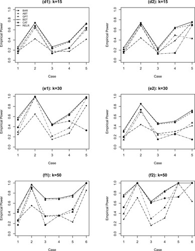
Figures 1 and 2 present the powers of the six tests for the 12 situations, (a1)–(f2), against the cases (specified in the 3rd column of Table 1.) From the results we can conclude that when the group size k is small $(\le 5)$, all tests yield a similar power pattern. This indicates that their performance very closes. When the group size k increases to moderate size like 10 or 15, the powers of BAR, ABT and RELR still show a similar pattern, and are higher than those of GPT, BDT and CAT. This indicates that BAR, ABT and RELR are superior to GPT, BDT and CAT. This superiority become more distinctive when the group size k increases to 30 or 50. For example, When k = 50, ${\mathit{\sigma }}^2=\lfloor (1,3,6,9,12);10\rfloor$, $n=\lfloor (3,4,5,4,3);10\rfloor$, the powers of CAT, BDT and GPT are 0.70, 0.517 and 0.309, respectively, while the powers of BAR, ABT and RELR are 0.827, 0.830, and 0.844, respectively (corresponding to case 4 of (f2) in Figure 2). Overall, RELR can effectively control the type I error, and its power is higher (or at least the same) than the other five tests for almost all configurations.

Figure 1. Simulation results for Settings (k = 2, 5, 10) corresponding to various cases. BAR: Bartlett's test (red line with filled square); ABT: Ma et al.'s test ; GPT: Liu & Xu's test; BDT: Bhandary & Dai's test; CAT: Gokpinar & Gokpinar's test; and LRT.

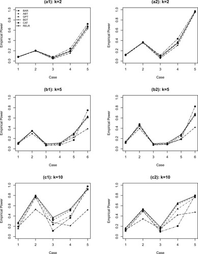
Figure 2. Simulation results for Settings (k = 15, 30, 50) corresponding to various cases. The caption is the same as in Figure 1.

5. Real data example

In this section, we analyse the dataset for the detrended particulate matter (pm${}_{10}$) of Maryland in 1990 by using the six tests to investigate the seasonal effect on pm${}_{10}$ variability. After removing missing observations, we have 88, 88, 97, and 74 observations within Spring, Summer, Fall, and Winter. Let ${\sigma }_i^2$ be their variances for i = 1, 2, 3, 4, respectively. This concern can then be formulated as the null hypothesis: $H_0:{\sigma }_1^2={\sigma }_2^2={\sigma }_3^2={\sigma }_4^2$.

We compute the p-value using the six tests with M = 10000. The corresponding p-values for BAR, ABT, GPT, CAT, RELR are $p_{\mathrm{BAR}}=0.0505$, $p_{\mathrm{ABT}}=0.0505$, $p_{\mathrm{GPT}}=0.0552$, $p_{\mathrm{CAT}}=0.0567$ and $p_{\mathrm{RELR}}=0.0495$, and BDT indicates that we fail to reject the null hypothesis for given $5\mathrm{\%}$ significant level. So all tests except the proposed RELR suggest that we could not reject the null hypothesis, while only RELR suggest a rejection, though these p-values are slightly different. Recalling our simulation results, we prefer the result based on RELR, and conclude that the variances among the four seasons are not homogeneous.

6. Concluding remarks

In this paper, we have proposed a procedure for calculating the p-value of the restrictive likelihood ratio test for variance homogeneity. The procedure is very easy to implement and performs promising. Given the optimality of the likelihood ratio principle, we conjecture that the test could be most efficient, which warrants a further investigation. This paper provides a means to calculate the p-value when it is difficult, if not impossible, to derive (asymptotic) distribution of the proposed test statistic. However, there is no a general guideline to reformulate $T_n$ in (2(2) $\begin{array}{rl}{T}_n& =(N-k)\log \left\{\frac{\sum _{i=1}^k(n_i-1)S_i^2}{N-k}\right\}\\ & -{\displaystyle \sum _{i=1}^k(n_i-1)\log S_i^2,}\end{array}$(2) ). So deriving a quantity similar to $T_{n,\mathrm{NEW}}$ may be case by case. Whether the proposed procedure can be applied to high-dimensional (in the sense of diverging with the sample size) situations is unclear and also warrants further research.

Disclosure statement

No potential conflict of interest was reported by the author(s).

Additional information

Funding

The research of Li was supported by Grant 11871294 from National Natural Science Foundation of China. Liang's research was partially supported by NSF grant DMS-1620898.

Notes on contributors

Juan Wang

Juan Wang is an assistant professor of School of Mathematics and Statistics at Qingdao University.

Xinmin Li

Xinmin Li is a professor of School of Mathematics and Statistics at Qingdao University.

Hua Liang

Hua Liang is a professor of Department of Statistics at George Washington University.

References

- Bartlett, M. S. (1937). Properties of sufficiency and statistical tests. Proceedings of the Royal Society. Series A, Mathematical and Physical Sciences, 160, 268–282. https://doi.org/https://doi.org/10.1098/rspa.1937.0109
- Bhandary, M., & Dai, H. (2009). An alternative test for the equality of variances for several populations when the underlying distributions are normal. Communications in Statistics Simulation and Computation, 38(1–2), 109–117. https://doi.org/https://doi.org/10.1080/03610918.2014.955110
- Bishop, D., & Nair, U. (1939). A note on certain methods of testing for the homogeneity of a set of estimated variances. Supplement to the Journal of the Royal Statistical Society, 6(1), 89–99. https://doi.org/https://doi.org/10.2307/2983627
- Boos, D. D., & Brownie, C. (1989). Bootstrap methods for testing homogeneity of variances. Technometrics, 31(1), 69–82. https://doi.org/https://doi.org/10.1080/00401706.1989.10488477
- Box, G. E. P. (1953). Non-normality and tests on variances. Biometrika, 40, 318–335. https://doi.org/https://doi.org/10.1093/biomet/40.3-4.318
- Brown, M. B., & Forsythe, A. B. (1974). Robust tests for the equality of variances. Journal of the American Statistical Association, 69(346), 364–367. https://doi.org/https://doi.org/10.1080/01621459.1974.10482955
- Cochran, W. G. (1951). Testing a linear relation among variances. Biometrics, 7, 17–32. https://doi.org/https://doi.org/10.2307/3001601
- Gokpinar, E., & Gokpinar, F. (2017). Testing equality of variances for several normal populations. Communications in Statistics Simulation and Computation, 46(1), 38–52. https://doi.org/https://doi.org/10.1080/03610918.2014.955110
- Hartley, H. O. (1940). Testing the homogeneity of a set of variances. Biometrika, 31, 249–255. https://doi.org/https://doi.org/10.1093/biomet/31.3-4.249
- Hartley, H. O. (1950). The maximum F-ratio as a short-cut test for heterogeneity of variance. Biometrika, 37, 308–312. https://doi.org/https://doi.org/10.2307/2332383
- Levene, H. (1960). Contributions to probability and statistics: Essays in honor of Harold Hotelling, In I. Olkin, S. G. Ghurye, W. Hoeffding, W. G. Madow, H. B. Mann (Eds.), Stanford studies in mathematics and statistics (Vol. 2). Stanford University Press.
- Liu, X., & Xu, X. (2010). A new generalized p-value approach for testing the homogeneity of variances. Statistics & Probability Letters, 80(19-20), 1486–1491. https://doi.org/https://doi.org/10.1016/j.spl.2010.05.017
- Ma, X.-B., Lin, F.-C., & Zhao, Y. (2015). An adjustment to the Bartlett's test for small sample size. Communications in Statistics Simulation and Computation, 44(1), 257–269. https://doi.org/https://doi.org/10.1080/03610918.2013.773347
- Pal, N., Lim, W. K., & Ling, C.-H. (2007). A computational approach to statistical inferences. Journal of Applied Probability and Statistics, 2(1), 13–35.
- Pardo, J., Pardo, M., Vicente, M., & Esteban, M. (1997). A statistical information theory approach to compare the homogeneity of several variances. Computational Statistics & Data Analysis, 24(4), 411–416. https://doi.org/https://doi.org/10.1016/S0167-9473(96)00080-1
- Teschendorff, A. E., & Widschwendter, M. (2012). Differential variability improves the identification of cancer risk markers in dna methylation studies profiling precursor cancer lesions. Bioinformatics (Oxford, England), 28, 1487–1494. https://doi.org/https://doi.org/10.1093/bioinformatics/bts170
- Tian, L. (2005). Inferences on the mean of zero-inflated lognormal data: The generalized variable approach. Statistics in Medicine, 24(20), 3223–3232. https://doi.org/https://doi.org/10.1002/(ISSN)1097-0258
- Tian, L. (2007). Inferences on standardized mean difference: The generalized variable approach. Statistics in Medicine, 26(5), 945–953. https://doi.org/https://doi.org/10.1002/(ISSN)1097-0258
- Weerahandi, S. (2004). Generalized inference in repeated measures. Wiley-Interscience [John Wiley & Sons].
- Wu, J., & Wong, A. C. M. (2003). A note on determining the p-value of Bartlett's test of homogeneity of variances. Communications in Statistics Theory and Methods, 32(1), 91–101. https://doi.org/https://doi.org/10.1081/STA-120017801