Empirical likelihood inference and goodness-of-fit test for logistic regression model under two-phase case-control sampling

ABSTRACT

Due to cost-effectiveness and high efficiency, two-phase case-control sampling has been widely used in epidemiology studies. We develop a semi-parametric empirical likelihood approach to two-phase case-control data under the logistic regression model. We show that the maximum empirical likelihood estimator has an asymptotically normal distribution, and the empirical likelihood ratio follows an asymptotically central chi-square distribution. We find that the maximum empirical likelihood estimator is equal to Breslow and Holubkov (1997)'s maximum likelihood estimator. Even so, the limiting distribution of the likelihood ratio, likelihood-ratio-based interval, and test are all new. Furthermore, we construct new Kolmogorov–Smirnov type goodness-of-fit tests to test the validation of the underlying logistic regression model. Our simulation results and a real application show that the likelihood-ratio-based interval and test have certain merits over the Wald-type counterparts and that the proposed goodness-of-fit test is valid.

KEYWORDS:

• Bootstrap
• case-control data
• empirical likelihood
• goodness-of-fit test
• two-phase case-control sampling

1. Introduction

Case-control studies have been conducted extensively in epidemiology and medical research, especially for rare diseases like cancer, as an easy and quick way of comparing treatments, or investigating the causes of disease. In a case-control study, the possible covariate information associated with diseases is collected for diseased and non-diseased individuals, and logistic regression models are usually used to model the relationship between the binary disease status and the covariate (Breslow & Day, 1980; Farewell, 1979; Prentice & Pyke, 1979). However, epidemiological and medical studies often require the collection of information on a large number of variables, including lifestyle, occupation, and environmental conditions. Certain variables are collected easily such as disease status and age in the social security system, but certain variables require a lot of cost, such as lifestyle. The difficulty can be overcome by employing a two-phase, two-stage or double sampling (Breslow et al., 2009; Neyman, 1938; Schaid et al., 2013; Thomas et al., 2013), where in the first phase, a relatively large number of individuals are sampled from a target population and information on variables that are easier to measure is collected. Together with a case-control sampling in the first phase, this leads to two-phase case-control sampling (Walker, 1982; White, 1982). At the first phase, cases and controls are sampled from a general population, and some stratifying information, such as a crude measure of exposure (e.g. disease or non-disease) is obtained. At the second phase, subsamples are selected within strata defined by disease status and by other stratifying information, and more refined information on exposure and other covariates is obtained for the subsample.

There have been many estimation methods dealing with logistic regression analysis of two-phase sampling data by making careful use of the information in the two sampling phases. Popular methods include the pseudo likelihood method (Breslow & Cain, 1988; Schill et al., 1993), the inverse probability weighted estimating method (Flanders & Greenland, 1991; Saegusa & Wellner, 2013), which takes the underlying sampling plan into account, and the maximum likelihood estimation method (Breslow & Holubkov, 1997; Lawless et al., 1999; Qin et al., 2015; Scott & Wild, 1997; Zhou et al., 2011). Among them, the methods developed by Lawless et al. (1999), Zhou et al. (2011), and Saegusa and Wellner (2013) are designed for general two-phase prospective data. As disclosed by Prentice and Pyke (1979), given usual case-control data, inferences for the odds ratio parameters based on prospective and retrospective likelihoods are equivalent. Therefore statistical methods designed for prospective data can usually be employed to make inference for retrospectively collected case-control data by taking them as if they were prospectively collected. Breslow and Holubkov (1997, p. 452) proved that this equivalence still holds for two-phase case-control data.

The existing works suggested to construct confidence intervals or conduct hypothesis testing for the odds ratio parameters based on the asymptotic normality of their proposed point estimators. This necessitates a consistent estimator for the accompanying asymptotic variance, which may have a very complicated form. In contrast, likelihood-ratio confidence intervals or tests are generally preferable as they are free of variance estimation. In addition, all the aforementioned methods for two-phase case-control data analysis are built on the logistic regression model assumption, whose mis-specification may have a detrimental or invalid effect on the subsequent analysis. Therefore it is necessary to check whether the logistic model is valid or not for two-phase case-control data.

Logistic regression models are commonly used in analysing binary data which arise in studying the relationship between diseases and environment or genetic characteristics. See for example, Breslow and Day (1980), Farewell (1979), and Prentice and Pyke (1979). Anderson (1979) noticed that the prospective logistic regression model is equivalent to the two sample exponential tilting model where one sample is corresponding to the covariate distribution for non-diseased group and the other one is the diseased group. With the standard case-control data, Qin and Zhang (1997) and Qin and Zhang (2005) proposed a Kolmogorov-Smirnov type statistic to test the validation of the logistic link function, where they implicitly used the empirical likelihood method (Owen, 1988) to estimate the underlying parameters. Qin (1998) found that the retrospective likelihood is equivalent to the empirical likelihood based on a density ratio model (Anderson, 1979, 1972). See Chen and Liu (2013), Cai et al. (2017), Diao et al. (2012), and Luo and Tsai (2012) for more about the density ratio model based on empirical likelihood.

Since the seminal work by Owen (1988), the empirical likelihood has become a popular nonparametric tool in statistical and economic literatures (Kitamura, 2006; Owen, 2001), as it has many nice properties paralleling to parametric likelihood. For example, empirical likelihood confidence regions are Bartlett correctable (DiCiccio et al., 1991; Liu & Chen, 2010), range preserving, transformation respecting, and do not require estimation of variance. It has the advantage of allowing the data to ‘speak for itself’ more and is more robust to slight mis-specification than parametric likelihood. Empirical likelihood has also found many applications in surveying sampling problems. Chen and Qin (1993) showed that empirical likelihood can effectively use auxiliary information. Chen et al. (2002) developed an elegant algorithm to implement the empirical likelihood method for finite-sample sampling problems. Zhao and Wu (2019) and Wu and Thompson (2020) provided a comprehensive review on the developments of empirical likelihood methods for complex surveys.

In this paper, we extend the empirical likelihood method for standard case-control data to two-phase case-control data. We find that the proposed maximum empirical likelihood point estimator is equal to Breslow and Holubkov (1997)'s maximum likelihood estimator under the logistic regression model. Unlike Breslow and Holubkov, (1997), we show that the empirical likelihood ratio statistic follows a limiting central chi-square distribution with a known degree of freedom. A remarkable advantage of the empirical likelihood-ratio test over the existing asymptotic-normality-based tests is that it is free of variance estimation. This makes it more convenient to construct empirical likelihood confidence regions or empirical likelihood-ratio tests, to test, for example, whether a covariate has a significant effect on disease occurrence. Furthermore, we construct new Kolmogorov-Smirnov type goodness-of-fit tests to test the validation of the logistic regression model.

The rest of this paper is organised as follows. Section 2 introduces the data and model assumptions, presents empirical likelihood, goodness-of-fit tests based on the density ratio model, and investigates their large-sample properties. Simulation results and a real-data analysis are provided in Sections 3 and 4, respectively. Finally, Section 5 contains some discussions. For clarity, all technical proofs are relegated to the Supplementary Material.

2. Semi-parametric likelihood

2.1. Data and model

Let D denote the disease status with D = 1 for a disease (case) and 0 for a non-disease (control), and X and Z denote two covariate vectors, where Z takes only finitely many values: $z_1,z_2,\dots ,z_J$. Suppose the probability of disease occurrence in the population of interest follows a linear logistic regression model (1) $\mathrm{p}\mathrm{r}(D=1|X=x,Z=z)=\frac{\exp ({\alpha }^{\ast }+x^{\mathrm{\top }}\text{β}+\gamma z)}{1+\exp ({\alpha }^{\ast }+x^{\mathrm{\top }}\text{β}+\gamma z)},$(1) where $\mathrm{\top }$ stands for transpose. Here and in what follows, we use $\mathrm{p}\mathrm{r}$ to denote probability density function with respect to the counting measure for a discrete random variable, and the Lebesgue measure for an absolutely continuous random variable. We collect data from the population under study by two-phase case-control sampling. At the first phase, fixed number $n_0$ of controls and $n_1$ of cases (sample 1) are drawn, independent of X and Z. Let $N_{ij}$ denote the observed number of individuals with ($D=i,Z=z_j$) for $i=0,1$ and $j=1,2,\dots ,J$. Then for each disease category, $(N_{i1},N_{i2},\dots ,N_{iJ})$ is a random vector following a multinomial distribution with parameter $n_i$ and $\mathrm{p}\mathrm{r}(z_j|D=i)$ ($j=1,2,\dots ,J$). At the second phase, within each Z-stratum of cases and controls in sample 1, a subsample is randomly selected, and exact or complete covariate measurements of the subsample are obtained (sample 2). Let $M_{ij}$'s denote the (random or non-random) sample sizes of the $2\times J$ validation strata. We observe a random sample $\{X_{ijk}:k=1,2,\dots ,M_{ij}\}$ for each pair $(i,j)$ with i = 0, 1 and $j=1,2,\dots ,J$. Conditioning on $\left\{M_{ij}\right\}$ and $\left\{N_{ij}\right\}$, all $X_{ijk}$ are assumed to be independent and $X_{ij1},X_{ij2},\dots ,X_{ij{M}_{ij}}$ are assumed to be identically distributed with probability density $\mathrm{p}\mathrm{r}(x|D=i,Z=z_j)$.

Given $\left\{M_{ij}\right\}$ and $\left\{N_{ij}\right\}$, the likelihood based on sample 2 is uninformative with respect to β. Therefore, the likelihood based on the two-phase case-control data is proportional to (2) $\prod _{i=0}^1\prod _{j=1}^J\left[\right\{\mathrm{p}\mathrm{r}(z_j|D=i){\}}^{N_{ij}}\prod _{k=1}^{M_{ij}}\mathrm{p}\mathrm{r}(x_{ijk}|D=i,z_j)],$(2) which is exactly the likelihood in Equation (2(2) $\prod _{i=0}^1\prod _{j=1}^J\left[\right\{\mathrm{p}\mathrm{r}(z_j|D=i){\}}^{N_{ij}}\prod _{k=1}^{M_{ij}}\mathrm{p}\mathrm{r}(x_{ijk}|D=i,z_j)],$(2) ) of Breslow and Holubkov (1997) for discrete covariate variables. This is the foundation of our empirical likelihood method. To proceed, we need to investigate $\mathrm{p}\mathrm{r}(z_j|D=i)$, and $\mathrm{p}\mathrm{r}(x_{ijk}|D=i,z_j)$ in Equation (2(2) $\prod _{i=0}^1\prod _{j=1}^J\left[\right\{\mathrm{p}\mathrm{r}(z_j|D=i){\}}^{N_{ij}}\prod _{k=1}^{M_{ij}}\mathrm{p}\mathrm{r}(x_{ijk}|D=i,z_j)],$(2) ) and study the relationship between them.

Let $\pi =\mathrm{p}\mathrm{r}(D=1)$. By Bayes's formula, we have $\begin{array}{rl}\mathrm{p}\mathrm{r}(x,z|D=1)& =\frac{1}{\pi }\mathrm{p}\mathrm{r}(D=1|x,z)\mathrm{p}\mathrm{r}(x,z),\\ \mathrm{p}\mathrm{r}(x,z|D=0)& =\frac{1}{1-\pi }\mathrm{p}\mathrm{r}(D=0|x,z)\mathrm{p}\mathrm{r}(x,z).\end{array}$It follows that $\begin{array}{rl}\frac{\mathrm{p}\mathrm{r}(x,z|D=1)}{\mathrm{p}\mathrm{r}(x,z|D=0)}& =\frac{1-\pi }{\pi }\frac{\mathrm{p}\mathrm{r}(D=1|x,z)}{\mathrm{p}\mathrm{r}(D=0|x,z)}\\ & =\frac{1-\pi }{\pi }\exp ({\alpha }^{\ast }+x^{\mathrm{\top }}\text{β}+\gamma z),\end{array}$where we have used Equation (1(1) $\mathrm{p}\mathrm{r}(D=1|X=x,Z=z)=\frac{\exp ({\alpha }^{\ast }+x^{\mathrm{\top }}\text{β}+\gamma z)}{1+\exp ({\alpha }^{\ast }+x^{\mathrm{\top }}\text{β}+\gamma z)},$(1) ). This implies that (3) $\begin{array}{rl}& \mathrm{p}\mathrm{r}(x,z|D=1)\\ & =\frac{1-\pi }{\pi }\exp ({\alpha }^{\ast }+x^{\mathrm{\top }}\text{β}+\gamma z)\cdot \mathrm{p}\mathrm{r}(x,z|D=0)\\ & =\exp (\alpha +x^{\mathrm{\top }}\text{β}+\gamma z)\cdot \mathrm{p}\mathrm{r}(x|D=0,z)\\ & \times \mathrm{p}\mathrm{r}(z|D=0),|d=1\end{array}$(3) where $\alpha ={\alpha }^{\ast }+\log \left\{\right(1-\pi \left)/\pi \right\}$.

Thus we immediately have (4) $\begin{array}{rl}& \mathrm{p}\mathrm{r}(z_j|D=1)\\ & =\int \mathrm{p}\mathrm{r}(x,z_j|D=1)\mathrm{d}x\\ & =\int \exp (\alpha +x^{\mathrm{\top }}\text{β}+\gamma z_j)\\ & \times \mathrm{p}\mathrm{r}(x|D=0,z_j)\mathrm{d}x\cdot \mathrm{p}\mathrm{r}(z_j|D=0)\\ & =\exp (\alpha +\gamma z_j-{\eta }_j)\cdot \mathrm{p}\mathrm{r}(z_j|D=0),|d=1\end{array}$(4) where ${\eta }_j=-\ln \{\int \exp (x^{\mathrm{\top }}\text{β})\cdot \mathrm{p}\mathrm{r}(x|D=0,z_j\left)\mathrm{d}x\right\}.$ Combining Equations (3(3) $\begin{array}{rl}& \mathrm{p}\mathrm{r}(x,z|D=1)\\ & =\frac{1-\pi }{\pi }\exp ({\alpha }^{\ast }+x^{\mathrm{\top }}\text{β}+\gamma z)\cdot \mathrm{p}\mathrm{r}(x,z|D=0)\\ & =\exp (\alpha +x^{\mathrm{\top }}\text{β}+\gamma z)\cdot \mathrm{p}\mathrm{r}(x|D=0,z)\\ & \times \mathrm{p}\mathrm{r}(z|D=0),|d=1\end{array}$(3) ) and (4(4) $\begin{array}{rl}& \mathrm{p}\mathrm{r}(z_j|D=1)\\ & =\int \mathrm{p}\mathrm{r}(x,z_j|D=1)\mathrm{d}x\\ & =\int \exp (\alpha +x^{\mathrm{\top }}\text{β}+\gamma z_j)\\ & \times \mathrm{p}\mathrm{r}(x|D=0,z_j)\mathrm{d}x\cdot \mathrm{p}\mathrm{r}(z_j|D=0)\\ & =\exp (\alpha +\gamma z_j-{\eta }_j)\cdot \mathrm{p}\mathrm{r}(z_j|D=0),|d=1\end{array}$(4) ) gives (5) $\begin{array}{rl}|zd& =1\mathrm{p}\mathrm{r}(x|D=1,z_j)=\frac{\mathrm{p}\mathrm{r}(x,z_j|D=1)}{\mathrm{p}\mathrm{r}(z_j|D=1)}\\ & =\exp ({\eta }_j+x^{\mathrm{\top }}\text{β})\cdot \mathrm{p}\mathrm{r}(x|D=0,z_j).\end{array}$(5) In summary, we have expressed $\mathrm{p}\mathrm{r}(z_j|D=i)$ and $\mathrm{p}\mathrm{r}(x_{ijk}|D=i,z_j)$ in Equation (2(2) $\prod _{i=0}^1\prod _{j=1}^J\left[\right\{\mathrm{p}\mathrm{r}(z_j|D=i){\}}^{N_{ij}}\prod _{k=1}^{M_{ij}}\mathrm{p}\mathrm{r}(x_{ijk}|D=i,z_j)],$(2) ) as functions of $\mathrm{p}\mathrm{r}(x|D=0,z_j)$ and some finite dimensional parameters.

2.2. Semi-parametric empirical likelihood

Putting the expressions in Equations (4(4) $\begin{array}{rl}& \mathrm{p}\mathrm{r}(z_j|D=1)\\ & =\int \mathrm{p}\mathrm{r}(x,z_j|D=1)\mathrm{d}x\\ & =\int \exp (\alpha +x^{\mathrm{\top }}\text{β}+\gamma z_j)\\ & \times \mathrm{p}\mathrm{r}(x|D=0,z_j)\mathrm{d}x\cdot \mathrm{p}\mathrm{r}(z_j|D=0)\\ & =\exp (\alpha +\gamma z_j-{\eta }_j)\cdot \mathrm{p}\mathrm{r}(z_j|D=0),|d=1\end{array}$(4) ) and (5(5) $\begin{array}{rl}|zd& =1\mathrm{p}\mathrm{r}(x|D=1,z_j)=\frac{\mathrm{p}\mathrm{r}(x,z_j|D=1)}{\mathrm{p}\mathrm{r}(z_j|D=1)}\\ & =\exp ({\eta }_j+x^{\mathrm{\top }}\text{β})\cdot \mathrm{p}\mathrm{r}(x|D=0,z_j).\end{array}$(5) ) into Equation (2(2) $\prod _{i=0}^1\prod _{j=1}^J\left[\right\{\mathrm{p}\mathrm{r}(z_j|D=i){\}}^{N_{ij}}\prod _{k=1}^{M_{ij}}\mathrm{p}\mathrm{r}(x_{ijk}|D=i,z_j)],$(2) ) and taking logarithm, we have a log-likelihood

$\begin{array}{rl}& \sum _{i=0}^1\sum _{j=1}^J[N_{ij}\log \{\mathrm{p}\mathrm{r}(z_j|D=i)\}+\sum _{k=1}^{M_{ij}}\log \{\mathrm{p}\mathrm{r}(x_{ijk}|D=i,z_j)\left\}\right]\\ & =\sum _{j=1}^J[N_{\cdot j}\log \left\{\mathrm{p}\mathrm{r}\right(z_j|D=0\left)\right\}+N_{1j}(\alpha +\gamma z_j-{\eta }_j)]\\ & +\sum _{j=1}^J[\sum _{i=0}^1\sum _{k=1}^{M_{ij}}\log \{\mathrm{p}\mathrm{r}(x_{ijk}|D=0,z_j)\}+\sum _{k=1}^{M_{1j}}({\eta }_j+x_{1jk}^{\mathrm{\top }}\text{β}\left)\right\}],\end{array}$

where $N_{\cdot j}=N_{0j}+N_{1j}$. As Z takes only finite values, let $q_j=\mathrm{p}\mathrm{r}(z_j|D=0)$. In the principle of empirical likelihood, we model the conditional distributions of X given $D=0$ and $Z=z_j$ by discrete distributions with support on the observations. Let $p_{ijk}=\mathrm{p}\mathrm{r}(x_{ijk}|D=0,Z=z_j)$. According to Equations (4(4) $\begin{array}{rl}& \mathrm{p}\mathrm{r}(z_j|D=1)\\ & =\int \mathrm{p}\mathrm{r}(x,z_j|D=1)\mathrm{d}x\\ & =\int \exp (\alpha +x^{\mathrm{\top }}\text{β}+\gamma z_j)\\ & \times \mathrm{p}\mathrm{r}(x|D=0,z_j)\mathrm{d}x\cdot \mathrm{p}\mathrm{r}(z_j|D=0)\\ & =\exp (\alpha +\gamma z_j-{\eta }_j)\cdot \mathrm{p}\mathrm{r}(z_j|D=0),|d=1\end{array}$(4) ) and (5(5) $\begin{array}{rl}|zd& =1\mathrm{p}\mathrm{r}(x|D=1,z_j)=\frac{\mathrm{p}\mathrm{r}(x,z_j|D=1)}{\mathrm{p}\mathrm{r}(z_j|D=1)}\\ & =\exp ({\eta }_j+x^{\mathrm{\top }}\text{β})\cdot \mathrm{p}\mathrm{r}(x|D=0,z_j).\end{array}$(5) ), the feasible $q_j$ and $p_{ijk}$ satisfy (6) $\{\begin{array}{l}{\displaystyle q_j\ge 0,p_{ijk}\ge 0,}\\ {\displaystyle \sum _{j=1}^J{q}_j=\sum _{j=1}^J{q}_j\exp (\alpha +\gamma z_j-{\eta }_j)=1,}\\ {\displaystyle \sum _{i=0}^1\sum _{k=1}^{M_{ij}}{p}_{ijk}=\sum _{i=0}^1\sum _{k=1}^{M_{ij}}{p}_{ijk}\exp ({\eta }_j+x_{ijk}^{\mathrm{\top }}\text{β})=1.}\end{array}$(6) With these preparations, the proposed semi-parametric empirical log-likelihood is $\begin{array}{rl}\tilde{\ell }& =\sum _{j=1}^J\{N_{\cdot j}\log \left(q_j\right)+N_{1j}(\alpha +\gamma z_j-{\eta }_j)\}\\ & +\sum _{j=1}^J\{\sum _{i=0}^1\sum _{k=1}^{M_{ij}}\log (p_{ijk})+\sum _{k=1}^{M_{1j}}({\eta }_j+x_{1jk}^{\mathrm{\top }}\text{β}\left)\right\}.\end{array}$We denote $N_{\cdot \cdot }=\sum _{j=1}^J{N}_{\cdot j}=n$ and $\theta =({\text{β}}^{\mathrm{\top }},\gamma ,{\eta }^{\mathrm{\top }}{)}^{\mathrm{\top }}$ with $\eta =({\eta }_1,\dots ,{\eta }_J{)}^{\mathrm{\top }}$. Inferences for $(\theta ,\alpha )$ are more conveniently made based on their profile likelihood, which is the maximum of $\tilde{\ell }$ with respect to $q_j$ and $p_{ijk}$ under the constraints in Equation (6(6) $\{\begin{array}{l}{\displaystyle q_j\ge 0,p_{ijk}\ge 0,}\\ {\displaystyle \sum _{j=1}^J{q}_j=\sum _{j=1}^J{q}_j\exp (\alpha +\gamma z_j-{\eta }_j)=1,}\\ {\displaystyle \sum _{i=0}^1\sum _{k=1}^{M_{ij}}{p}_{ijk}=\sum _{i=0}^1\sum _{k=1}^{M_{ij}}{p}_{ijk}\exp ({\eta }_j+x_{ijk}^{\mathrm{\top }}\text{β})=1.}\end{array}$(6) ). By the Lagrange multiplier method, the maximum is achieved at (7) $\{\begin{array}{l}{\displaystyle q_j=\frac{N_{\cdot j}}{N_{\cdot \cdot }}\frac{1}{1+\lambda \{\exp (\alpha +\gamma z_j-{\eta }_j)-1\}},}\\ j=1,2,\dots ,J,\\ {\displaystyle p_{ijk}=\frac{1}{M_{\cdot j}}\frac{1}{1+{\lambda }_j\{\exp ({\eta }_j+x_{ijk}^{\mathrm{\top }}\text{β})-1\}},}\\ i=0,1,k=1,2,\dots ,M_{ij},\end{array}$(7) where $M_{\cdot j}=M_{0j}+M_{1j}$, $\lambda =\lambda (\theta ,\alpha )$, and ${\lambda }_j={\lambda }_j(\theta ,\alpha )$ are the solutions to $\{\begin{array}{l}{\displaystyle \sum _{j=1}^J\frac{N_{\cdot j}}{N_{\cdot \cdot }}\frac{\exp (\alpha +\gamma z_j-{\eta }_j)-1}{1+\lambda \{\exp (\alpha +\gamma z_j-{\eta }_j)-1\}}=0,}\\ {\displaystyle \sum _{i=0}^1\sum _{k=1}^{M_{ij}}\frac{\exp ({\eta }_j+x_{ijk}^{\mathrm{\top }}\text{β})-1}{1+{\lambda }_j\{\exp ({\eta }_j+x_{ijk}^{\mathrm{\top }}\text{β})-1\}}=0,}\\ j=1,2,\dots ,J.\end{array}$This immediately leads to the profile empirical log-likelihood function of $(\theta ,\alpha )$, $\begin{array}{rl}& \ell (\theta ,\alpha )\\ & =C^{\ast }-\sum _{j=1}^J{N}_{\cdot j}\log [1+\lambda \{\exp (\alpha +\gamma z_j-{\eta }_j)-1\left\}\right]\\ & +\sum _{j=1}^J{N}_{1j}(\alpha +\gamma z_j-{\eta }_j)\\ & -\sum _{j=1}^J\sum _{i=0}^1\sum _{k=1}^{M_{ij}}\log [1+{\lambda }_j\{\exp ({\eta }_j+x_{ijk}^{\mathrm{\top }}\text{β})-1\left\}\right]\\ & +\sum _{j=1}^J\sum _{k=1}^{M_{1j}}({\eta }_j+x_{1jk}^{\mathrm{\top }}\text{β}),\end{array}$where $C^{\ast }=\sum _{j=1}^J\{N_{\cdot j}\log (N_{\cdot j}/N_{\cdot \cdot })+\sum _{i=0}^1{M}_{ij}\log (1/M_{\cdot j}\left)\right\}$does not depend on $(\theta ,\alpha )$.

We propose to estimate $(\theta ,\alpha )$ by the maximum likelihood estimator (MLE), $(\hat{\theta },\hat{\alpha })=\arg \underset{\theta ,\alpha }{max}\ell (\theta ,\alpha ).$ The parameter α is merely a normalised parameter and generally of no importance. We may further profile α out and make inference for θ through $\ell \left(\theta \right)=\underset{\alpha }{max}\ell (\theta ,\alpha )$. Here, we abuse the notation $\ell (\cdot )$, whose meaning is clear from the context. It is seen that the MLE of θ based on $\ell \left(\theta \right)$ is still $\hat{\theta }$.

Lemma 2.1

Our maximum empirical likelihood estimator for $(\text{β},\gamma )$ is identical to the maximum likelihood estimator of Breslow and Holubkov (1997) when their method takes the stratum variable into account.

Lemma 2.1 indicates that numerically our point estimator is equal to Breslow and Holubkov (1997)'s MLE. Even so, the density ratio model based on empirical likelihood framework for two-phase sampling data is new in the literature, and as far as we know, likelihood-ratio-based inferences under this setting have not been investigated yet in the literature. Breslow and Holubkov (1997)'s statistical inferences (interval estimation and hypothesis testing) for the unknown parameters were based on the asymptotic normality of the MLE.

2.3. Asymptotics

In this section, we establish the limiting distributions of the MLE $\hat{\theta }$ and the semi-parametric likelihood-ratio statistic. First of all, we introduce some conditions on the sampling plan and the population under study.

Condition (C1)

There exist positive constants ${\lambda }_0^{\ast },c^{\ast },c_j^{\ast },{\lambda }_{j0}$ ($j=1,2,\dots ,J$) such that $c\equiv M_{\cdot \cdot }/n=c^{\ast }+o_p\left(1\right)$, ${\lambda }_0\equiv n_1/n={\lambda }_0^{\ast }+o\left(1\right)$, $c_j\equiv M_{\cdot j}/n=c_j^{\ast }+o_p\left(1\right)$, and ${\lambda }_{j0}\equiv M_{1j}/M_{\cdot j}={\lambda }_{j0}^{\ast }+o_p\left(1\right)$ as n tends to infinity.

Condition (C1) guarantees that the sizes of the subsamples in all the strata are comparable, and they are also comparable with the case and control samples in the first phase. Otherwise, the strata with negligible sample sizes is simply discarded from our theoretical analysis.

Condition (C2)

The integral $\int \exp \left(x^{\mathrm{\top }}\text{β}\right)f_j\left(x\right)\mathrm{d}x$ is finite for β in a neighbourhood of ${\text{β}}_0$ and a neighbourhood of 0 for all $j=1,2,\dots ,J$, where $f_j\left(x\right)=\mathrm{p}\mathrm{r}(x|D=0,Z=z_j)$.

Under Condition (C2), the moment generating functions of $\mathrm{p}\mathrm{r}(x|D=0,Z=z_j)$, namely $\int \exp \left(x^{\mathrm{\top }}\text{β}\right)\times \mathrm{p}\mathrm{r}(x|D=0,Z=z_j)\mathrm{d}x$, are well defined in a neighbourhood of the origin. Therefore in the stratum with D = 0 and $Z=z_j$, the covariate X has all finite-order moments. If model (1(1) $\mathrm{p}\mathrm{r}(D=1|X=x,Z=z)=\frac{\exp ({\alpha }^{\ast }+x^{\mathrm{\top }}\text{β}+\gamma z)}{1+\exp ({\alpha }^{\ast }+x^{\mathrm{\top }}\text{β}+\gamma z)},$(1) ) is true, it follows from Equation (5(5) $\begin{array}{rl}|zd& =1\mathrm{p}\mathrm{r}(x|D=1,z_j)=\frac{\mathrm{p}\mathrm{r}(x,z_j|D=1)}{\mathrm{p}\mathrm{r}(z_j|D=1)}\\ & =\exp ({\eta }_j+x^{\mathrm{\top }}\text{β})\cdot \mathrm{p}\mathrm{r}(x|D=0,z_j).\end{array}$(5) ) that $\begin{array}{rl}& \int \exp \left(x^{\mathrm{\top }}\text{β}\right)\mathrm{p}\mathrm{r}(x|D=1,Z=z_j)\mathrm{d}x\\ & =\int \exp ({\eta }_j+x^{\mathrm{\top }}{\text{β}}_0)\exp \left(x^{\mathrm{\top }}\text{β}\right)\\ & \times \mathrm{p}\mathrm{r}(x|D=0,Z=z_j)\mathrm{d}x.\end{array}$The finiteness of $\int \exp \left(x^{\mathrm{\top }}\text{β}\right)\mathrm{p}\mathrm{r}(x|D=0,Z=z_j)\mathrm{d}x$ in a neighbourhood of ${\text{β}}_0$ implies that the moment generating functions of $\mathrm{p}\mathrm{r}(x|D=1,Z=z_j)$ are also finite in a neighbourhood of the origin. Consequently, conditioning on D = 0 and $Z=z_j$, the covariate X also has all finite-order moments.

The expression of the asymptotic variance of $\hat{\theta }$ is rather complicated. For ease of presentation, some notations are needed. We use ${\theta }_0=({\text{β}}_0^{\mathrm{\top }},{\gamma }_0,{\eta }_0^{\mathrm{\top }}{)}^{\mathrm{\top }}$ with ${\eta }_0=({\eta }_{10},\dots ,{\eta }_{J0})$ to denote the true value of θ under model (1(1) $\mathrm{p}\mathrm{r}(D=1|X=x,Z=z)=\frac{\exp ({\alpha }^{\ast }+x^{\mathrm{\top }}\text{β}+\gamma z)}{1+\exp ({\alpha }^{\ast }+x^{\mathrm{\top }}\text{β}+\gamma z)},$(1) ), and define $a_j=\exp ({\alpha }_0+{\gamma }_0{z}_j-{\eta }_{j0})$ and $A_j=1+{\lambda }_0(a_j-1)$ for $1\le j\le J$. Write $B^{\otimes 2}=B{B}^{\mathrm{\top }}$ for any vector of matrix B. Let $\begin{array}{rl}{D}_j& =\frac{1}{{\lambda }_{j0}}\int \frac{1-\exp ({\eta }_{j0}+x^{\mathrm{\top }}{\text{β}}_0)}{1+{\lambda }_{j0}\{\exp ({\eta }_{j0}+x^{\mathrm{\top }}{\text{β}}_0)-1\}}{f}_j\left(x\right)\mathrm{d}x,\\ D_{j0}& =\int \frac{\exp ({\eta }_{j0}+x^{\mathrm{\top }}{\text{β}}_0)}{1+{\lambda }_{j0}\{\exp ({\eta }_{j0}+x^{\mathrm{\top }}{\text{β}}_0)-1\}}{f}_j\left(x\right)\mathrm{d}x,\\ D_{j1}& =\int \frac{\exp ({\eta }_{j0}+x^{\mathrm{\top }}{\text{β}}_0)}{1+{\lambda }_{j0}\{\exp ({\eta }_{j0}+x^{\mathrm{\top }}{\text{β}}_0)-1\}}x{f}_j\left(x\right)\mathrm{d}x,\\ D_{j2}& =\int \frac{\exp ({\eta }_{j0}+x^{\mathrm{\top }}{\text{β}}_0)}{1+{\lambda }_{j0}\{\exp ({\eta }_{j0}+x^{\mathrm{\top }}{\text{β}}_0)-1\}}{x}^{\otimes 2}{f}_j\left(x\right)\mathrm{d}x,\end{array}$and $\begin{array}{rl}{E}_0& =\sum _{j=1}^J\frac{q_j{a}_j}{A_j},E_1=\sum _{j=1}^J\frac{q_j{a}_j}{A_j}{z}_j,\\ E_2& =\sum _{j=1}^J\frac{q_j{a}_j}{A_j}{z}_j^{\otimes 2},\end{array}$where $q_j=\mathrm{p}\mathrm{r}(z_j|D=0)$. The following matrix plays an important role in the asymptotic normality of $\hat{\theta }$: $V_n=\left(V_{ij}\right),$ where $\begin{array}{rl}{V}_{1,1}& ={\lambda }_0(1-{\lambda }_0)(E_2-\frac{E_1^{\otimes 2}}{E_0}),V_{1,2}=0,\\ V_{2,2}& =\sum _{j=1}^{J}c{c}_j\left\{{\lambda }_{j0}\right(1-{\lambda }_{j0})D_{j2}+\frac{D_{j1}^{\otimes 2}}{D_j}\},\\ V_{2+j,2+j}& =c{c}_j\frac{D_{j0}}{D_j}+q_j\frac{{\lambda }_0(1-{\lambda }_0)a_j}{A_j}\\ & -\frac{{\lambda }_0(1-{\lambda }_0)}{E_0}\frac{q_j^2{a}_j^2}{A_j^2},\\ V_{2+j,2+k}& =-\frac{q_j{a}_j}{A_j}\frac{q_k{a}_k}{A_k}\frac{{\lambda }_0(1-{\lambda }_0)}{E_0},1\le j\ne k\le J,\\ V_{1,2+j}& =-\frac{q_j{a}_j}{A_j}{\lambda }_0(1-{\lambda }_0)(z_j-\frac{E_1}{E_0}),\\ V_{2,2+j}& =c{c}_j\frac{D_{j1}}{D_j}.\end{array}$It is worth noting that the quantities ${\lambda }_0,{\lambda }_{j0},c$, and $c_j$ all depend on n.

Theorem 2.1

Suppose that model (1(1) $\mathrm{p}\mathrm{r}(D=1|X=x,Z=z)=\frac{\exp ({\alpha }^{\ast }+x^{\mathrm{\top }}\text{β}+\gamma z)}{1+\exp ({\alpha }^{\ast }+x^{\mathrm{\top }}\text{β}+\gamma z)},$(1) ) and Conditions (C1) and (C2) all hold. As $n\to \mathrm{\infty }$, if $V_n$ converges to a nonsingular matrix $V_{\ast }$, then (I) $\sqrt{n}(\hat{\theta }-{\theta }_0)$ converges in distribution to a multivariate normal distribution with mean zero and variance-covariance matrix $V_{\ast }$; (II) the semi-parametric likelihood ratio $2\left\{l\right(\hat{\theta })-l({\theta }_0\left)\right\}$ has a limiting ${\chi }_K^2$ distribution, where K is the dimension of θ.

The proof of Theorem 2.1 also implies that the likelihood ratio statistic for any subvector of θ also follows an asymptotic chi-square distribution with a known degree of freedom. A key and interesting problem in case-control study is to check whether some or all of the covariates X and Z have significant effects on the disease occurrence D, or construct confidence intervals for their coefficients. Under the framework of the proposed semi-parametric empirical likelihood, we propose to construct confidence intervals and hypothesis tests based on the likelihood ratio function calibrated by its limiting chi-square distribution. Theorem 2.1 theoretically guarantees that for θ or any of its subvectors, our likelihood-ratio confidence intervals have asymptotically correct coverage probabilities, and our likelihood ratio tests have asymptotically correct type I errors.

2.4. Goodness-of-fit test

The previous nice properties of the proposed semi-parametric likelihood method are achieved under the assumption of model (1(1) $\mathrm{p}\mathrm{r}(D=1|X=x,Z=z)=\frac{\exp ({\alpha }^{\ast }+x^{\mathrm{\top }}\text{β}+\gamma z)}{1+\exp ({\alpha }^{\ast }+x^{\mathrm{\top }}\text{β}+\gamma z)},$(1) ). Possible misspecifications of this model pose a validation risk on the semi-parametric likelihood-based inference. Therefore, it is necessary for checking the logistic regression model. We achieve this purpose by checking models (4(4) $\begin{array}{rl}& \mathrm{p}\mathrm{r}(z_j|D=1)\\ & =\int \mathrm{p}\mathrm{r}(x,z_j|D=1)\mathrm{d}x\\ & =\int \exp (\alpha +x^{\mathrm{\top }}\text{β}+\gamma z_j)\\ & \times \mathrm{p}\mathrm{r}(x|D=0,z_j)\mathrm{d}x\cdot \mathrm{p}\mathrm{r}(z_j|D=0)\\ & =\exp (\alpha +\gamma z_j-{\eta }_j)\cdot \mathrm{p}\mathrm{r}(z_j|D=0),|d=1\end{array}$(4) ) and (5(5) $\begin{array}{rl}|zd& =1\mathrm{p}\mathrm{r}(x|D=1,z_j)=\frac{\mathrm{p}\mathrm{r}(x,z_j|D=1)}{\mathrm{p}\mathrm{r}(z_j|D=1)}\\ & =\exp ({\eta }_j+x^{\mathrm{\top }}\text{β})\cdot \mathrm{p}\mathrm{r}(x|D=0,z_j).\end{array}$(5) ) simultaneously, since roughly speaking the validation of the assumption of model (1(1) $\mathrm{p}\mathrm{r}(D=1|X=x,Z=z)=\frac{\exp ({\alpha }^{\ast }+x^{\mathrm{\top }}\text{β}+\gamma z)}{1+\exp ({\alpha }^{\ast }+x^{\mathrm{\top }}\text{β}+\gamma z)},$(1) ) is equivalent to that of both models (4(4) $\begin{array}{rl}& \mathrm{p}\mathrm{r}(z_j|D=1)\\ & =\int \mathrm{p}\mathrm{r}(x,z_j|D=1)\mathrm{d}x\\ & =\int \exp (\alpha +x^{\mathrm{\top }}\text{β}+\gamma z_j)\\ & \times \mathrm{p}\mathrm{r}(x|D=0,z_j)\mathrm{d}x\cdot \mathrm{p}\mathrm{r}(z_j|D=0)\\ & =\exp (\alpha +\gamma z_j-{\eta }_j)\cdot \mathrm{p}\mathrm{r}(z_j|D=0),|d=1\end{array}$(4) ) and (5(5) $\begin{array}{rl}|zd& =1\mathrm{p}\mathrm{r}(x|D=1,z_j)=\frac{\mathrm{p}\mathrm{r}(x,z_j|D=1)}{\mathrm{p}\mathrm{r}(z_j|D=1)}\\ & =\exp ({\eta }_j+x^{\mathrm{\top }}\text{β})\cdot \mathrm{p}\mathrm{r}(x|D=0,z_j).\end{array}$(5) ).

Similar to Qin and Zhang (1997), we construct Kolmogrov–Smirnov type tests for models (4(4) $\begin{array}{rl}& \mathrm{p}\mathrm{r}(z_j|D=1)\\ & =\int \mathrm{p}\mathrm{r}(x,z_j|D=1)\mathrm{d}x\\ & =\int \exp (\alpha +x^{\mathrm{\top }}\text{β}+\gamma z_j)\\ & \times \mathrm{p}\mathrm{r}(x|D=0,z_j)\mathrm{d}x\cdot \mathrm{p}\mathrm{r}(z_j|D=0)\\ & =\exp (\alpha +\gamma z_j-{\eta }_j)\cdot \mathrm{p}\mathrm{r}(z_j|D=0),|d=1\end{array}$(4) ) and (5(5) $\begin{array}{rl}|zd& =1\mathrm{p}\mathrm{r}(x|D=1,z_j)=\frac{\mathrm{p}\mathrm{r}(x,z_j|D=1)}{\mathrm{p}\mathrm{r}(z_j|D=1)}\\ & =\exp ({\eta }_j+x^{\mathrm{\top }}\text{β})\cdot \mathrm{p}\mathrm{r}(x|D=0,z_j).\end{array}$(5) ). Let ${\hat{q}}_j$ and ${\hat{p}}_{ijk}$ be the fitted probability weights obtained by plugging the MLE $(\hat{\theta },\hat{\alpha })$ in Equation (7(7) $\{\begin{array}{l}{\displaystyle q_j=\frac{N_{\cdot j}}{N_{\cdot \cdot }}\frac{1}{1+\lambda \{\exp (\alpha +\gamma z_j-{\eta }_j)-1\}},}\\ j=1,2,\dots ,J,\\ {\displaystyle p_{ijk}=\frac{1}{M_{\cdot j}}\frac{1}{1+{\lambda }_j\{\exp ({\eta }_j+x_{ijk}^{\mathrm{\top }}\text{β})-1\}},}\\ i=0,1,k=1,2,\dots ,M_{ij},\end{array}$(7) ) and ${\tilde{q}}_{ij}=N_{ij}/N_{i\cdot }$. A measure of the departure from the assumption of model (4(4) $\begin{array}{rl}& \mathrm{p}\mathrm{r}(z_j|D=1)\\ & =\int \mathrm{p}\mathrm{r}(x,z_j|D=1)\mathrm{d}x\\ & =\int \exp (\alpha +x^{\mathrm{\top }}\text{β}+\gamma z_j)\\ & \times \mathrm{p}\mathrm{r}(x|D=0,z_j)\mathrm{d}x\cdot \mathrm{p}\mathrm{r}(z_j|D=0)\\ & =\exp (\alpha +\gamma z_j-{\eta }_j)\cdot \mathrm{p}\mathrm{r}(z_j|D=0),|d=1\end{array}$(4) ) is ${\mathrm{\Delta }}_1=\underset{j}{max}(|{\mathrm{\Delta }}_{10j}|+|{\mathrm{\Delta }}_{11j}|),$ where (8) $\begin{array}{rl}{\mathrm{\Delta }}_{10j}& =n^{1/2}({\tilde{q}}_{0j}-{\hat{q}}_j),\\ {\mathrm{\Delta }}_{11j}& =n^{1/2}\{{\tilde{q}}_{1j}-{\hat{q}}_j\exp (\hat{\alpha }+z_j^{\mathrm{\top }}\hat{\gamma }-{\hat{\eta }}_j\left)\right\}.\end{array}$(8)

Theorem 2.2

Under the same conditions as Theorem 2.1, ${\mathrm{\Delta }}_{10j}$ and ${\mathrm{\Delta }}_{11j}$ have a jointly normal limiting distribution with mean zero.

We consider testing the goodness-of-fit of model (5(5) $\begin{array}{rl}|zd& =1\mathrm{p}\mathrm{r}(x|D=1,z_j)=\frac{\mathrm{p}\mathrm{r}(x,z_j|D=1)}{\mathrm{p}\mathrm{r}(z_j|D=1)}\\ & =\exp ({\eta }_j+x^{\mathrm{\top }}\text{β})\cdot \mathrm{p}\mathrm{r}(x|D=0,z_j).\end{array}$(5) ). We are using $F_{ij}\left(x\right)$ to denote the distribution function of $X_{ijk}$ given D = i and $Z=z_j$, i = 0, 1 and $j=1,2,\dots ,J$. With the fitted values ${\hat{p}}_{ijk}$, the empirical likelihood (EL) estimators of $F_{ij}\left(x\right)$ are $\begin{array}{rl}{\hat{F}}_{0j}\left(x\right)& =\sum _{i=0}^1\sum _{k=1}^{M_{ij}}{\hat{p}}_{ijk}I(x_{ijk}\le x),\\ {\hat{F}}_{1j}\left(x\right)& =\sum _{i=0}^1\sum _{k=1}^{M_{ij}}{\hat{p}}_{ijk}\exp ({\hat{\eta }}_j+x_{ijk}^{\mathrm{\top }}\widehat{\text{β}})I(x_{ijk}\le x),\end{array}$where the inequality $x_{ijk}\le x$ holds element-wise. Let ${\tilde{F}}_{ij}\left(x\right)$ denote the empirical distribution corresponding to the subsample $\{x_{ij1},x_{ij2},\dots ,x_{ij{M}_{ij}}\}$ for fixed i and j. A measure of the departure from the assumption of model (5(5) $\begin{array}{rl}|zd& =1\mathrm{p}\mathrm{r}(x|D=1,z_j)=\frac{\mathrm{p}\mathrm{r}(x,z_j|D=1)}{\mathrm{p}\mathrm{r}(z_j|D=1)}\\ & =\exp ({\eta }_j+x^{\mathrm{\top }}\text{β})\cdot \mathrm{p}\mathrm{r}(x|D=0,z_j).\end{array}$(5) ) is ${\mathrm{\Delta }}_{2j}=\underset{x}{sup}|{\mathrm{\Delta }}_{20j}\left(x\right)|+\underset{x}{sup}|{\mathrm{\Delta }}_{21j}\left(x\right)|,$ where (9) $\begin{array}{rl}{\mathrm{\Delta }}_{20j}\left(x\right)& =n^{1/2}\left\{{\hat{F}}_{0j}\right(x)-{\tilde{F}}_{0j}(x\left)\right\},\\ {\mathrm{\Delta }}_{21j}\left(x\right)& =n^{1/2}\left\{{\hat{F}}_{1j}\right(x)-{\tilde{F}}_{1j}(x\left)\right\}.\end{array}$(9)

Theorem 2.3

Under the same conditions as Theorem 2.1, ${\mathrm{\Delta }}_{20j}\left(x\right)$ and ${\mathrm{\Delta }}_{21j}\left(x\right)$ all converge weakly to Brown motions with mean zero.

An overall measure of departures from the assumption of models (4(4) $\begin{array}{rl}& \mathrm{p}\mathrm{r}(z_j|D=1)\\ & =\int \mathrm{p}\mathrm{r}(x,z_j|D=1)\mathrm{d}x\\ & =\int \exp (\alpha +x^{\mathrm{\top }}\text{β}+\gamma z_j)\\ & \times \mathrm{p}\mathrm{r}(x|D=0,z_j)\mathrm{d}x\cdot \mathrm{p}\mathrm{r}(z_j|D=0)\\ & =\exp (\alpha +\gamma z_j-{\eta }_j)\cdot \mathrm{p}\mathrm{r}(z_j|D=0),|d=1\end{array}$(4) ) and (5(5) $\begin{array}{rl}|zd& =1\mathrm{p}\mathrm{r}(x|D=1,z_j)=\frac{\mathrm{p}\mathrm{r}(x,z_j|D=1)}{\mathrm{p}\mathrm{r}(z_j|D=1)}\\ & =\exp ({\eta }_j+x^{\mathrm{\top }}\text{β})\cdot \mathrm{p}\mathrm{r}(x|D=0,z_j).\end{array}$(5) ) is (10) $\begin{array}{rl}\mathrm{\Delta }& =\underset{j}{max}(|{\mathrm{\Delta }}_{10j}|+|{\mathrm{\Delta }}_{11j}|+\underset{x}{sup}|{\mathrm{\Delta }}_{20j}(x)|\\ & +\underset{x}{sup}|{\mathrm{\Delta }}_{21j}\left(x\right)|),\end{array}$(10) where ${\mathrm{\Delta }}_{10j}$, ${\mathrm{\Delta }}_{11j}$, ${\mathrm{\Delta }}_{20j}$, and ${\mathrm{\Delta }}_{21j}$ are all defined in Equations (8(8) $\begin{array}{rl}{\mathrm{\Delta }}_{10j}& =n^{1/2}({\tilde{q}}_{0j}-{\hat{q}}_j),\\ {\mathrm{\Delta }}_{11j}& =n^{1/2}\{{\tilde{q}}_{1j}-{\hat{q}}_j\exp (\hat{\alpha }+z_j^{\mathrm{\top }}\hat{\gamma }-{\hat{\eta }}_j\left)\right\}.\end{array}$(8) ) and (9(9) $\begin{array}{rl}{\mathrm{\Delta }}_{20j}\left(x\right)& =n^{1/2}\left\{{\hat{F}}_{0j}\right(x)-{\tilde{F}}_{0j}(x\left)\right\},\\ {\mathrm{\Delta }}_{21j}\left(x\right)& =n^{1/2}\left\{{\hat{F}}_{1j}\right(x)-{\tilde{F}}_{1j}(x\left)\right\}.\end{array}$(9) ). The limiting distribution of Δ is too complicated to be conveniently used in practice. We use a bootstrap procedure (Efron, 1979) to approximate it or the p-value.

Before introducing the bootstrap procedure, we briefly review the original two-phase case-control data. The data in the first phase consists of $n_0$ controls (D = 0) and $n_1$ cases (D = 1). There are $N_{ij}$ data in the strata with D = i and $Z=z_j$, for $i=0,1$ and $j=1,2,\dots ,J$. Fix i = 0 or 1, the vector $(N_{i1},N_{i2},\dots ,N_{iJ})$ follows a multinomial distribution with parameters $n_i$ and $\left\{\mathrm{p}\mathrm{r}\right(z_j|D=i):j=1,2,\dots ,J\}$. For each pair $(i,j)$, the data in the second phase are $M_{ij}$ independent and identically distributed observations $X_{ij1},X_{ij2},\dots ,X_{ij{M}_{ij}}$ from $\mathrm{p}\mathrm{r}(x|D=i,Z=z_j)$. If $M_{ij}$ are non-random integers, they are pre-specified. Otherwise, they are often determined by sampling proportions, say $r_{ij}\in (0,1)$, and then $M_{ij}=N_{ij}{r}_{ij}$. We use $q_{ij}$ and $F_{ij}\left(x\right)$ to denote $\mathrm{p}\mathrm{r}(Z=z_j|D=i)$ and $\mathrm{p}\mathrm{r}(x|D=i,Z=z_j)$, respectively. And we have shown that $q_{1j}=q_{0j}\exp ({\alpha }_0+{\gamma }_0{z}_j-{\eta }_0)$ under model (4(4) $\begin{array}{rl}& \mathrm{p}\mathrm{r}(z_j|D=1)\\ & =\int \mathrm{p}\mathrm{r}(x,z_j|D=1)\mathrm{d}x\\ & =\int \exp (\alpha +x^{\mathrm{\top }}\text{β}+\gamma z_j)\\ & \times \mathrm{p}\mathrm{r}(x|D=0,z_j)\mathrm{d}x\cdot \mathrm{p}\mathrm{r}(z_j|D=0)\\ & =\exp (\alpha +\gamma z_j-{\eta }_j)\cdot \mathrm{p}\mathrm{r}(z_j|D=0),|d=1\end{array}$(4) ), and $F_{1j}\left(x\right)={\int }_{-\mathrm{\infty }}^x\exp ({\eta }_0+x^{\mathrm{\top }}{\text{β}}_0)\mathrm{d}{F}_{0j}\left(x\right)$ under model (5(5) $\begin{array}{rl}|zd& =1\mathrm{p}\mathrm{r}(x|D=1,z_j)=\frac{\mathrm{p}\mathrm{r}(x,z_j|D=1)}{\mathrm{p}\mathrm{r}(z_j|D=1)}\\ & =\exp ({\eta }_j+x^{\mathrm{\top }}\text{β})\cdot \mathrm{p}\mathrm{r}(x|D=0,z_j).\end{array}$(5) ).

Our bootstrap procedure to approximate the p-value of the goodness-of-fit test for model (1(1) $\mathrm{p}\mathrm{r}(D=1|X=x,Z=z)=\frac{\exp ({\alpha }^{\ast }+x^{\mathrm{\top }}\text{β}+\gamma z)}{1+\exp ({\alpha }^{\ast }+x^{\mathrm{\top }}\text{β}+\gamma z)},$(1) ) based on Δ is as follows.

1. Based on the original two-phase case-control data, do the following steps:

   1. Calculate the EL estimator $(\hat{\theta },\hat{\alpha })=\arg \underset{\theta ,\alpha }{max}\ell (\theta ,\alpha )$

   2. Calculate the EL estimators ${\hat{q}}_{0j}={\hat{q}}_j$, ${\hat{q}}_{1j}={\hat{q}}_j\exp (\hat{\alpha }+z_j^{\mathrm{\top }}\hat{\gamma }-{\hat{\eta }}_j)\}$, ${\hat{F}}_{0j}\left(x\right)$, and ${\hat{F}}_{1j}\left(x\right)={\int }_{-\mathrm{\infty }}^x\exp (\hat{\eta }+t^{\mathrm{\top }}\widehat{\text{β}})\mathrm{d}{\hat{F}}_{0j}\left(t\right)$ under model (1(1) $\mathrm{p}\mathrm{r}(D=1|X=x,Z=z)=\frac{\exp ({\alpha }^{\ast }+x^{\mathrm{\top }}\text{β}+\gamma z)}{1+\exp ({\alpha }^{\ast }+x^{\mathrm{\top }}\text{β}+\gamma z)},$(1) ).

   3. Calculate the test statistic Δ defined in Equation (10(10) $\begin{array}{rl}\mathrm{\Delta }& =\underset{j}{max}(|{\mathrm{\Delta }}_{10j}|+|{\mathrm{\Delta }}_{11j}|+\underset{x}{sup}|{\mathrm{\Delta }}_{20j}(x)|\\ & +\underset{x}{sup}|{\mathrm{\Delta }}_{21j}\left(x\right)|),\end{array}$(10) ).

2. Generate a bootstrap sample based on the original sample.

   1. Generate $n_0$ z-values from the discrete distribution defined by $P(Z=z_j)={\hat{q}}_{0j}$, and $n_1$ z-values from the discrete distribution defined by $P(Z=z_j)={\hat{q}}_{1j}$. We suppose that there are $N_{ij}^{\ast }$ observations with D = i and $Z=z_j$. Then the bootstrap sample in the first phase is $S_1^{\ast }=\left\{N_{ij}^{\ast }\right\}$.

   2. At the strata with D = i and $Z=z_j$, draw $M_{ij}$ (the non-random case) or $M_{ij}=N_{ij}^{\ast }{r}_{ij}$ (the random case) observations from ${\hat{F}}_{ij}\left(x\right)$. The resulting observations constitute a bootstrap sample in the second phase, i.e. $S_2^{\ast }=\left\{\right(x_{ij1}^{\ast },\dots ,x_{ij{M}_{ij}}^{\ast }):i=0,1;j=1,\dots ,J\}$.

3. Calculate the test statistic by replacing the original sample with the bootstrap sample, which consists of $S_1^{\ast }$ and $S_2^{\ast }$. We denote the resulting test statistic by ${\mathrm{\Delta }}^{\ast }$.

4. Repeat steps 2 and 3 B times (e.g. B = 200). We denote the resulting B test statistics by ${\mathrm{\Delta }}_1^{\ast },\dots ,{\mathrm{\Delta }}_B^{\ast }$. The bootstrap p-value of the test based on Δ is $\left(1/B\right)\sum _{i=1}^{B}I({\mathrm{\Delta }}_i^{\ast }\ge \mathrm{\Delta })$.

3. Simulation study

By simulations, we compare our method with Breslow and Holubkov (1997)'s method from two aspects: interval estimation and hypothesis testing. We also investigate the finite-sample performance of the proposed goodness-of-fit test for model (1(1) $\mathrm{p}\mathrm{r}(D=1|X=x,Z=z)=\frac{\exp ({\alpha }^{\ast }+x^{\mathrm{\top }}\text{β}+\gamma z)}{1+\exp ({\alpha }^{\ast }+x^{\mathrm{\top }}\text{β}+\gamma z)},$(1) ).

3.1. Interval estimation and hypothesis testing about θ

Our proposed interval estimators and hypothesis tests about θ are both based on the semi-parametric empirical likelihood-ratio function. In contrast, the counterparts of Breslow and Holubkov (1997) are both based on Wald's method and their maximum likelihood estimators, which are implemented with the R package missreg3 in R version 2.15.3. We use ELR and Wald to denote our and their methods, respectively.

We generate two-phase case-control data from model (1(1) $\mathrm{p}\mathrm{r}(D=1|X=x,Z=z)=\frac{\exp ({\alpha }^{\ast }+x^{\mathrm{\top }}\text{β}+\gamma z)}{1+\exp ({\alpha }^{\ast }+x^{\mathrm{\top }}\text{β}+\gamma z)},$(1) ), with $x=(x_1,x_2,x_3)$ following the trivariate standard normal distribution, and $z=\left[s\right]$, where $s\sim U(0,2)$ and $\left[s\right]$ denotes the nearest integer to s. The true parameter value of ${\alpha }_{\ast }$ is set to $-4$ in all cases; and the rest model parameters $(\gamma ,{\text{β}}_1,{\text{β}}_2,{\text{β}}_3)$ are to be determined. We set $n_0=n_1=200$, $n_0=n_1=100$, and the number of simulations to 2000.

We first compare the ELR and Wald methods from interval estimation. We construct confidence intervals for γ, $(\gamma ,{\text{β}}_1)$, $(\gamma ,{\text{β}}_1,{\text{β}}_2)$, and $(\gamma ,{\text{β}}_1,{\text{β}}_2,{\text{β}}_3)$ at confidence levels 90%, 95%, and 99%. Two groups of parameter values are considered: $(\gamma ,{\text{β}}_1,{\text{β}}_2,{\text{β}}_3)=(0,0,1,2)$ and $(1,0,1,2)$. The simulated coverage probabilities of the ELR and Wald intervals are tabulated in Tables 1 and 2. It is seen that both intervals have very accurate coverage probabilities. The ELR interval has slight under-coverage whereas the Wald interval has over-coverage when the total sample size is as small as $n_0=n_1=100$. The under-coverage of the ELR interval is at most 2%; however, the over-coverage of the Wald interval can be as large as 4.5%, in the case of $(\gamma ,{\text{β}}_1,{\text{β}}_2)$ at the 90% confidence level. Both of their coverage accuracies improve as the sample size increases to 200.

Table 1. Coverage probabilities (%) of the Wald and ELR confidence intervals with $n_0=n_1=100$.

		γ	$(\gamma ,{\text{β}}_1)$	$(\gamma ,{\text{β}}_1,{\text{β}}_2)$	$(\gamma ,{\text{β}}_1,{\text{β}}_2,{\text{β}}_3)$
Level (%)	Method	The true parameter value is $(0,0,1,2)$
90	ELR	88.20	88.60	88.90	87.90
	Wald	90.85	93.60	94.50	92.75
95	ELR	93.95	93.85	94.20	93.35
	Wald	96.30	97.75	97.55	96.60
99	ELR	98.60	98.25	98.40	98.10
	Wald	99.50	99.55	99.60	99.25
		The true parameter value is $(1,0,1,2)$
90	ELR	89.05	88.95	87.20	88.25
	Wald	92.05	92.25	92.50	92.25
95	ELR	94.10	94.25	93.15	93.65
	Wald	96.05	96.20	96.40	96.05
99	ELR	98.65	98.60	98.35	97.60
	Wald	99.30	99.45	99.35	98.75

Table 2. Coverage probabilities (%) of the Wald and ELR confidence intervals with $n_0=n_1=200$.

		γ	$(\gamma ,{\text{β}}_1)$	$(\gamma ,{\text{β}}_1,{\text{β}}_2)$	$(\gamma ,{\text{β}}_1,{\text{β}}_2,{\text{β}}_3)$
Level (%)	Method	The true parameter value is $(0,0,1,2)$
90	ELR	89.50	89.85	89.85	87.85
	Wald	90.55	91.60	92.40	90.90
95	ELR	94.15	94.25	94.35	93.35
	Wald	95.40	96.25	96.40	94.95
99	ELR	98.70	98.40	98.60	97.85
	Wald	99.25	99.40	99.40	98.60
		The true parameter value is $(1,0,1,2)$
90	ELR	88.10	88.80	89.05	88.95
	Wald	88.90	90.85	90.80	91.25
95	ELR	93.70	94.40	94.35	94.40
	Wald	94.60	95.70	95.70	95.05
99	ELR	98.85	98.85	98.85	98.20
	Wald	99.25	99.40	99.05	98.70

Next, we study the finite-sample performance of the ELR and Wald tests. We consider the hypothesis testing problems in Examples 3.1 and 3.2, respectively, which are concerned with the same four parameter combinations. The effect of the strata variable Z is set to zero in the null hypotheses of Example 3.1 and nonzero in those of Example 3.2, respectively.

Example 3.1

Consider four groups of hypotheses ($k=0,1,\dots ,4$):

(A1)	${\mathrm{H}}_0:\gamma =0\leftrightarrow {\mathrm{H}}_1:\gamma =0.3\times k$, where $({\text{β}}_1,{\text{β}}_2,{\text{β}}_3)=(-1,1,2)$;
(A2)	${\mathrm{H}}_0:(\gamma ,{\text{β}}_1)=(0,0)\leftrightarrow {\mathrm{H}}_1:(\gamma ,{\text{β}}_1)=(0.35,-0.1)\times k$, where $({\text{β}}_2,{\text{β}}_3)=(1,2)$;
(A3)	${\mathrm{H}}_0:(\gamma ,{\text{β}}_1,{\text{β}}_2)=(0,0,0)\leftrightarrow {\mathrm{H}}_1:(\gamma ,{\text{β}}_1,{\text{β}}_2)=(0.35,-0.1,-0.1)\times k$, where ${\text{β}}_3=2$;
(A4)	${\mathrm{H}}_0:(\gamma ,{\text{β}}_1,{\text{β}}_2,{\text{β}}_3)=(0,0,0,0)\leftrightarrow {\mathrm{H}}_1:(\gamma ,{\text{β}}_1,{\text{β}}_2)=(0.15,-0.1,-0.1,-0.1)\times k$.

Example 3.2

Consider four groups of hypotheses ($k=0,1,\dots ,4$):

(B1)	${\mathrm{H}}_0:\gamma =1\leftrightarrow {\mathrm{H}}_1:\gamma =1+0.3\times k$, where $({\text{β}}_1,{\text{β}}_2,{\text{β}}_3)=(-1,1,2)$;
(B2)	${\mathrm{H}}_0:(\gamma ,{\text{β}}_1)=(1,1)\leftrightarrow {\mathrm{H}}_1:(\gamma ,{\text{β}}_1)=(1,1)+(0.25,-0.1)\times k$, where $({\text{β}}_2,{\text{β}}_3)=(1,2)$;
(B3)	${\mathrm{H}}_0:(\gamma ,{\text{β}}_1,{\text{β}}_2)=(1,1,1)\leftrightarrow {\mathrm{H}}_1:(\gamma ,{\text{β}}_1,{\text{β}}_2)=(1,1,1)+(0.35,-0.05,-0.05)\times k$, where ${\text{β}}_3=2$;
(B4)	${\mathrm{H}}_0:(\gamma ,{\text{β}}_1,{\text{β}}_2,{\text{β}}_3)=(1,1,1,1)\leftrightarrow {\mathrm{H}}_1:(\gamma ,{\text{β}}_1,{\text{β}}_2,{\text{β}}_3)=(1,1,1,1)+(0.1,-0.1,-0.1,-0.1)\times k$.

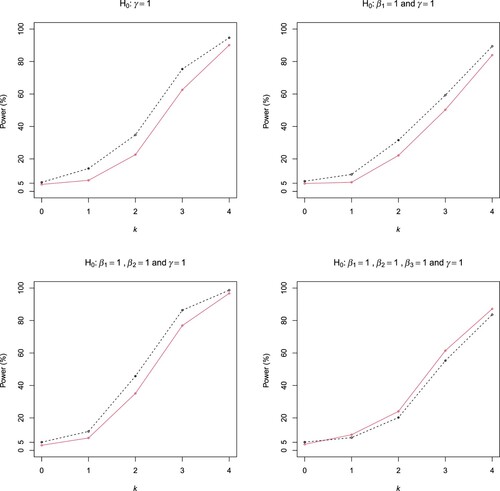
The simulated rejection rates of the ELR and Wald tests in all the cases are displayed in Figures 1 and 2. The rejection rates are simulated type I errors when k = 0 and are simulated powers when k>0. It is seen that both tests have well controlled type I errors. The ELR test is uniformly more powerful than the Wald test in all cases except case (B4), where the two tests have very close powers. The power gain of the ELR test over the Wald test is as large as 10%, for example, in case (B1).

Figure 1. Rejection probabilities of the ELR (dashed line) and Wald (solid line) tests in Scenarios (A1) and (A2) (First row), and (A3) and (A4) (Second row) of Example 3.1.

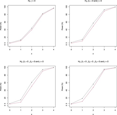
Figure 2. Rejection probabilities of the ELR (dashed line) and Wald (solid line) tests in Scenarios (B1) and (B2) (First row), and (B3) and (B4) (Second row) of Example 3.2.

Overall, compared with the Wald method, the ELR interval has comparable accuracy while the ELR tests are often more powerful. It is worth mentioning that a clear advantage of the ELR test over the Wald test is that it does not need a variance estimation. The price is numerical optimisation, which is not an issue in the current era of high-speed computer.

3.2. Goodness-of-fit test for logistic regression model

In this subsection, we investigate the finite-sample performance of the proposed goodness-of-fit test for the logistic regression model (1(1) $\mathrm{p}\mathrm{r}(D=1|X=x,Z=z)=\frac{\exp ({\alpha }^{\ast }+x^{\mathrm{\top }}\text{β}+\gamma z)}{1+\exp ({\alpha }^{\ast }+x^{\mathrm{\top }}\text{β}+\gamma z)},$(1) ); its null distribution is approximated by the bootstrap procedure in Section 2.4. No competitors are taken into account because to the best of our knowledge this problem has never been studied in the context of two-phase case-control data.

We set $n_0=n_1=500$ and the number of simulations to 1000. We also suppose that Z takes three different values with $z_1=0.15$, $z_2=0.2$, and $z_3=0.3$. Given D, we generate Z from the distribution function $q_{ij}=\mathrm{p}\mathrm{r}(Z=z_j|D=i)$ such that $q_{01}=\exp (-z_1\gamma )$, $q_{02}=\exp (-z_2\gamma )$, $q_{03}=1-\exp (-z_1\gamma )-\exp (-z_2\gamma )$, $q_{11}=\exp (\alpha -{\eta }_1)$, $q_{12}=\exp (\alpha -{\eta }_2)$, and $q_{13}=\exp (\alpha -{\eta }_3+z_3\gamma )\{1-\exp (-z_1\gamma )-\exp (-z_2\gamma \left)\right\}$. We consider two types of x: univariate and bivariate, corresponding to Examples 3.3 and 3.4, respectively.

Example 3.3

Suppose that X is univariate, and its conditional distributions given D and Z are $X|(D=0,Z=z_1)\sim N(0,1)$, $X|(D=0,Z=z_2)\sim N(1,1)$, $X|(D=0,Z=z_3)\sim N(1/2,1)$, $X|(D=1,Z=z_1)\sim N(\text{β},{\sigma }_1^2)$, $X|(D=1,Z=z_2)\sim N(\text{β}+1,{\sigma }_1^2)$, and $X|(D=1,X=z_3)\sim N(\text{β}+1/2,{\sigma }_1^2)$. It is verified that ${\eta }_1=-0.5{\text{β}}^2$, ${\eta }_2=-0.5{\text{β}}^2-\text{β}$, and ${\eta }_3=-0.5{\text{β}}^2-0.5\text{β}$. We set $\text{β}=0.2$, $\gamma =6$, and ${\sigma }_1^2=1+k\times 0.4$ for $k=0,\dots ,4$.

When k = 0 or ${\sigma }_1^2=1$, it is verified that $\mathrm{p}\mathrm{r}(x|D=1,z_1=0.15)/\mathrm{p}\mathrm{r}(x|D=0,z_1=0.15)=\exp ({\eta }_1+x\text{β})$, $\mathrm{p}\mathrm{r}(x|D=1,z_2=0.2)/\mathrm{p}\mathrm{r}(x|D=0,z_2=0.2)=\exp ({\eta }_2+x\text{β})$, and $\mathrm{p}\mathrm{r}(x|D=1,z_3=0.3)/\mathrm{p}\mathrm{r}(x|D=0,z_2=0.3)=\exp ({\eta }_3+x\text{β})$. In other words, model (1(1) $\mathrm{p}\mathrm{r}(D=1|X=x,Z=z)=\frac{\exp ({\alpha }^{\ast }+x^{\mathrm{\top }}\text{β}+\gamma z)}{1+\exp ({\alpha }^{\ast }+x^{\mathrm{\top }}\text{β}+\gamma z)},$(1) ) is true when ${\sigma }_1^2=1$. The rejection proportion of the proposed test is a simulated type I error. When $k\ne 0$ or ${\sigma }_1^2\ne 1$, the linear logistic model assumption is not true any longer, and the rejection proportions are simulated powers of the proposed test.

Example 3.4

Let $\mathbf{1}=(1,1{)}^{\mathrm{\top }}$, $I_2=\mathrm{d}\mathrm{i}\mathrm{a}\mathrm{g}\left(\mathbf{1}\right)$, and $\mathbf{c}=(1/2,1/2{)}^{\mathrm{\top }}$. Suppose that X is bivariate and given D and Z, its conditional distributions are $X|(D=0,Z=z_1)\sim N_2(0\times \mathbf{1},I_2)$, $X|(D=0,Z=z_2)\sim N_2(\mathbf{1},I_2)$, $X|(D=0,Z=z_3)\sim N_2(0.5\times \mathbf{1},I_2)$, $X|(D=1,Z=z_1)\sim N_2(\text{β},{\sigma }_2^2\times I_2)$, $X|(D=1,Z=z_2)\sim N_2(\text{β}+\mathbf{1},{\sigma }_2^2\times I_2)$, and $X|(D=1,X=z_3)\sim N_2(\text{β}+0.5\times \mathbf{1},{\sigma }_2^2\times I_2)$. It follows that ${\eta }_1=-0.5{\text{β}}^{\mathrm{\top }}\text{β}$, ${\eta }_2=-0.5{\text{β}}^{\mathrm{\top }}\cdot (\text{β}+\mathbf{1}\mathbf{)}$, and ${\eta }_3=-0.5{\text{β}}^{\mathrm{\top }}(\text{β}+\mathbf{c}\mathbf{)}$. We set $\text{β}=(-1.2,1.2{)}^{\mathrm{\top }}$, $\gamma =6$, and ${\sigma }_2^2=1+k$ for $k=0,\dots ,4$.

Similar to Example 3.3, model (1(1) $\mathrm{p}\mathrm{r}(D=1|X=x,Z=z)=\frac{\exp ({\alpha }^{\ast }+x^{\mathrm{\top }}\text{β}+\gamma z)}{1+\exp ({\alpha }^{\ast }+x^{\mathrm{\top }}\text{β}+\gamma z)},$(1) ) is true in Example 3.4 when k = 0 or ${\sigma }_2^2=1$ and is violated otherwise. Table 3 presents the simulated rejection rates of the proposed goodness-of-fit test at the 5% significance level for Examples 3.3 and 3.4. Again the results corresponding to k = 0 are type I errors and others are powers. The proposed test has type I errors 6.1% and 5.1%, both of which are well controlled under the 5% significance level. As k increases from 1 to 4, the linear logistic model is violated more and more severely, and the proposed test has increasing powers to nearly 100%. This provides evidence for the consistency and validation of the proposed test for testing goodness-of-fit of model (1(1) $\mathrm{p}\mathrm{r}(D=1|X=x,Z=z)=\frac{\exp ({\alpha }^{\ast }+x^{\mathrm{\top }}\text{β}+\gamma z)}{1+\exp ({\alpha }^{\ast }+x^{\mathrm{\top }}\text{β}+\gamma z)},$(1) ).

Table 3. Rejection probabilities (%) of model checking of Examples 3.3 and 3.4.

$k=$	0	1	2	3	4
Example 3.3	6.1	10.5	39.8	75.4	93.4
Example 3.4	5.1	14.5	39.9	71.2	90.5

4. Real-data analysis

In this section, we illustrate the proposed semi-parametric empirical likelihood method by analysing a simulated two-phase data set constructed by the actual National Wilms Tumor Study Group (NWTSG). See D'Angio et al. (1989), Breslow and Chatterjee (1999), and Green et al. (1998) for more description about the data. A problem of interest is to investigate whether there exists an association between treatment outcomes and tumour histology in 4028 children, who were diagnosed with the embryonal cancer of the kidney, known as Wilms tumour. The outcome variable of interest in this study is the relapse, which takes 1 (the patient's condition has deteriorated) and 0 (the patient's condition has improved) values. The covariates of interest include institution histology or IH (0 if favourable, 1 unfavourable), central histology or CH (0 if favourable, 1 unfavourable), stage ((1,0,0) if stage-II, (0,1,0) if stage-III, and (0,0,1) if stage-IV), and age (in months).

Two types of histology measurements are available in the study. First, according to histology, the classification of tumours as favourable and unfavourable is based on the pathologist at the hospital where the children were admitted. As the study data came from many different hospitals, institutional histology may be prone to errors due to the subjective judgments of different pathologists. Thus, the NWTGS re-evaluated histology using a central pathologist recruited for the entire study which was called central histology, the second measurement for histology available in the study. The covariate IH has no prognostic value once the account has been taken into central histology. Even so, we take it as a stratum variable in two-phase case-control sampling. The histologic diagnosis results are tabulated in Table 4.

Table 4. IH and outcome for Wilms tumour.

IH	Relapsed	Non-relapsed
Favourable	415	3,207
Unfavourable	156	250

We take the data in Table 4 as if they were prospective with a prevalence of 14.1%. In the first phase, we randomly choose $N_1$ cases from relapsed population and $N_0$ controls from non-relapsed population, where $N_1=500$ and $N_0=500$. Then we classified the $N_1$ cases and $N_0$ controls according to their IH condition. In the second phase, we randomly choose $M_{ij}=N_{ij}/3$ $(i=0,1;j=1,2)$ observations in each subpopulation.

Before applying model (1(1) $\mathrm{p}\mathrm{r}(D=1|X=x,Z=z)=\frac{\exp ({\alpha }^{\ast }+x^{\mathrm{\top }}\text{β}+\gamma z)}{1+\exp ({\alpha }^{\ast }+x^{\mathrm{\top }}\text{β}+\gamma z)},$(1) ) and our empirical likelihood method to analyse the data, we use the proposed goodness-of-fit test to check the validation of the linear logistic regression model. The resulting p-value of 0.71 provides no evidence against this model at 5% significance level.

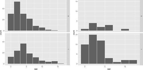
Wilms tumours have no clear cause, but there are some potential factors that affect the risk. Besides stage, age may be an important prognostic factor for Wilms tumour. Figure 3 displays the histograms of age at all the four combinations of outcome and stratum variables. We see that the four condition distributions of age are quite different from each other, which intuitively implies that age is probably associated with the outcome. Formally the ELR (p-value of 0.0014) and Wald (p-value of 0.0020) tests both provide strong evidence for the association of age and outcome at the 5% significance level, although the evidence from the ELR test is stronger. We also test whether stage and IH are associated with the outcome. For stage, the ELR test gives a positive answer (p-value of 0.0498) while the Wald test gives a negative answer (p-value of 0.0534). Both tests give negative answers (their p-values are 0.2082 and 0.1871, respectively) for IH and give positive answers (their p-values are 0 and 0.001, respectively) for CH.

Figure 3. Histograms of Age in different combinations of outcome (Row 1, relapses or cases; Row 2, non-relapses or controls) and the stratum variable (IH; Column 1, unfavourable; Column 2, favourable).

The point and interval estimators of the coefficients of all the covariates are presented in Table 5. The coefficient of age, 0.1316, is positive, indicating that older people are more likely to relapse than younger people. The coefficient of CH is significantly nonzero while no evidence supports that of IH is nonzero. This result is consistent with that IH has no prognostic value once account has been taken into central histology. The interval estimators confirm the above hypothesis testing results: namely age and CH are important factors to relapse.

Table 5. Results of regression parameter estimates in Wilms tumour study.

		Confidence interval
Variable	Estimate	Wald	ELR
Intercept	−1.3026	(−1.7570, −0.8482)	(−1.8399, −0.7932)
CH	3.1958	(1.5867, 4.8049)	(1.7909, 5.1445)
Age	0.1316	(0.0483, 0.2150)	(0.0500, 0.2173)
Stage-II	0.6399	(0.0080, 1.2718)	(0.0093, 1.2759)
Stage-III	0.3685	(−0.2929, 1.0298)	(−0.2970, 1.0294)
Stage-IV	1.0052	(0.2196, 1.7908)	(0.2272, 1.8053)
IH	−0.9811	(−2.4389, 0.4766)	(−2.9375, 0.5030)

5. Discussion

This paper develops an empirical likelihood approach to two-phase case-control data. We require that the covariate Z takes finite different values because it is regarded as a stratification variable. Two issues about the covariate or strata are worth discussing. First, if Z is continuous, we need to transform it to a discrete variable U taking finite different values. Then we may proceed with U in place of Z, although there may be information loss in doing so. Alternatively, we may take U as a stratification variable, and take the raw variable Z as a subvector of X in model (1(1) $\mathrm{p}\mathrm{r}(D=1|X=x,Z=z)=\frac{\exp ({\alpha }^{\ast }+x^{\mathrm{\top }}\text{β}+\gamma z)}{1+\exp ({\alpha }^{\ast }+x^{\mathrm{\top }}\text{β}+\gamma z)},$(1) ), so that the effect of Z on the disease can still be studied. Second, the performance of the proposed method depends on the approximation accuracy of its large-sample properties and may be undermined if some sample sizes of the $2J$ strata are too small. A large number of strata may make some strata have very small sizes. To avoid this problem, we recommend stratifying the data such that there are at least 5 observations in each strata and the number of strata in each disease status is small, say 5. Strata with too small sizes should be merged to be large strata so that the asymptotic normality of the proposed estimator and the limiting chisquare distribution of the proposed likelihood ratio have acceptable accuracy.

Acknowledgments

The authors thank the Editor, the Associate Editor, and the two anonymous referees for helpful comments and suggestions that have led to significant improvements in the paper.

Disclosure statement

No potential conflict of interest was reported by the author(s).

Additional information

Funding

The research was supported by the National Natural Science Foundation of China [grant number 11771144], the State Key Program of National Natural Science Foundation of China [grant number 71931004], [grant number 32030063], the development fund for Shanghai talents, and the 111 project (B14019).

Notes on contributors

Zhen Sheng

Zhen Sheng is a PhD candidate in School of Statistics, Faculty of Economic and Management, East China Normal University, China. She received her master degree in Statistics in 2018 from Qufu Normal University, China. Her research interests include case-control study, Genome-wide association study, and experimental design.

Yukun Liu

Yukun Liu is a Professor in School of Statistics, Faculty of Economic and Management, East China Normal University, China. He received his PhD in Statistics in 2009 from Nankai University, China. His research is focused on empirical likelihood and its applications to case-control data, capture-recapture data, selection biased data, and finite mixture models.

Jing Qin

Jing Qin is a Mathematical Statistician in the Biostatistics Research Branch of the National Institute of Allergy and Infectious Diseases (NIAID), USA. He received his PhD in Statistics from the University of Waterloo in 1992. His research interests include empirical likelihood, case-control study, length bias sampling, survival analysis, missing data, causal inference, and survey sampling.

References

- Anderson, J. A. (1972). Separate sample logistic discrimination. Biometrika, 59(1), 19–35. https://doi.org/10.1093/biomet/59.1.19
- Anderson, J. A. (1979). Multivariate logistic compounds. Biometrika, 66, 17–26. https://doi.org/10.2307/2335237
- Breslow, N. E., & Cain, K. C. (1988). Logistic regression for two-stage case-control data. Biometrika, 75(1), 11–20. https://doi.org/10.1093/biomet/75.1.11
- Breslow, N. E., & Chatterjee, N. (1999). Design and analysis of two-phase studies with binary outcome applied to Wilms tumour prognosis. Applied Statistics, 48(4), 457–468. https://doi.org/10.1111/1467-9876.00165
- Breslow, N., & Day, N. E. (1980). Statistical methods in cancer research. Volume 1. The analysis of case-control studies. IARC Scientific Publications.
- Breslow, N. E., & Holubkov, R. (1997). Maximum likelihood estimation of logistic regression parameters under two-phase, outcome-dependent sampling. Journal of the Royal Statistical Society Series B, 59(2), 447–461. https://doi.org/10.1111/rssb.1997.59.issue-2
- Breslow, N. E., Lumley, T., Ballantyne, C. M., Chambless, L. E., & Kulich, M. (2009). Improved Horvitz-Thompson estimation of model parameters from two-phase stratified samples: Applications in epidemiology. Statistics in Biosciences, 1(1), 32–49. https://doi.org/10.1007/s12561-009-9001-6
- Cai, S., Chen, J., & Zidek, J. V. (2017). Hypothesis testing in the presence of multiple samples under density ratio models. Statistica Sinica, 27, 761–783. https://doi.org/10.5705/ss.2014.168
- Chen, J., & Liu, Y. (2013). Quantile and quantile-function estimations under density ratio model. Annals of Statistics, 41(3), 1669–1692. https://doi.org/10.1214/13-AOS1129
- Chen, J., & Qin, J. (1993). Empirical likelihood estimation for finite populations and the effective usage of auxiliary information. Biometrika, 80(1), 107–116. https://doi.org/10.1093/biomet/80.1.107
- Chen, J., Sitter, R. R., & Wu, C. (2002). Using empirical likelihood methods to obtain range restricted weights in regression estimators for surveys. Biometrika, 89(1), 230–237. https://doi.org/10.1093/biomet/89.1.230
- D'Angio, G. J., Breslow, N., Beckwith, J. B., Evans, A., Baum, H., Fernbach, D., Hrabovsky, E., Jones, B., & Kelalis, P. (1989). Treatment of Wilms' tumour. Results of the third national Wilms' tumor study. Cancer, 64(2), 349–360. https://doi.org/10.1002/(ISSN)1097-0142
- Diao, G., Ning, J., & Qin, J. (2012). Maximum likelihood estimation for semiparametric density ratio model. The International Journal of Biostatistics, 8(1). https://doi.org/10.1515/1557-4679.1372
- DiCiccio, T., Hall, P., & Romano, J. (1991). Empirical likelihood is Bartlett-correctable. The Annals of Statistics, 19(2), 1053–1061. https://doi.org/10.1214/aos/1176348137
- Efron, B. (1979). Bootstrap methods: Another look at the jackknife. The Annals of Statistics, 7(1), 1–26. https://doi.org/10.1214/aos/1176344552
- Farewell, V. (1979). Some results on the estimation of logistic models based on retrospective data. Biometrika, 66(1), 27–32. https://doi.org/10.1093/biomet/66.1.27
- Flanders, W. D., & Greenland, S. (1991). Analytic methods for two-stage case-control studies and other stratified designs. Statistics in Medicine, 10(5), 739–747. https://doi.org/10.1002/(ISSN)1097-0258
- Green, D. M., Breslow, N. E., Beckwith, J. B., Finklestein, J. Z., Grundy, P. E., P. R. Thomas, Kim, T., Shochat, S. J., Haase, G. M., Ritchey, M. L., Kelalis, P. P., & D'Angio, G. J. (1998). Comparison between single-dose and divided-dose administration of dactinomycin and doxorubicin for patients with Wilms' tumor: A report from the national Wilms' tumor study group. Journal of Clinical Oncology: Official Journal of the American Society of Clinical Oncology, 16(1), 237–245. https://doi.org/10.1200/JCO.1998.16.1.237
- Kitamura, Y. (2006). Empirical likelihood methods in econometrics: theory and practice. Discussion Paper 1569. Cowles Foundation.
- Lawless, J. F., Kalbfleisch, J. D., & Wild, C. J. (1999). Semiparametric methods for response-selective and missing data problems in regression. Journal of the Royal Statistical Society Series B, 61(2), 413–438. https://doi.org/10.1111/rssb.1999.61.issue-2
- Liu, Y., & Chen, J. (2010). Adjusted empirical likelihood with high-order precision. The Annals of Statistics, 38(3), 1341–1362. https://doi.org/10.1214/09-AOS750
- Luo, X., & Tsai, W. Y. (2012). A proportional likelihood ratio model. Biometrika, 99(1), 211–222. https://doi.org/10.1093/biomet/asr060
- Neyman, J. (1938). Contribution to the theory of sampling human populations. Journal of the American Statistical Association, 33(201), 101–116. https://doi.org/10.1080/01621459.1938.10503378
- Owen, A. B. (1988). Empirical likelihood ratio confidence intervals for a single functional. Biometrika, 75(2), 237–249. https://doi.org/10.1093/biomet/75.2.237
- Owen, A. B. (2001). Empirical likelihood. Chapman and Hall.
- Prentice, R. L., & Pyke, R. (1979). Logistic disease incidence models and case-control studies. Biometrika, 66(3), 403–411. https://doi.org/10.1093/biomet/66.3.403
- Qin, J. (1998). Inferences for case-control and semiparametric two-sample density ratio models. Biometrika, 85(3), 619–630. https://doi.org/10.1093/biomet/85.3.619
- Qin, J., & Zhang, B. (1997). A goodness-of-fit test for logistic regression models based on case-control data. Biometrika, 84(3), 609–618. https://doi.org/10.1093/biomet/84.3.609
- Qin, J., & Zhang, B. (2005). Density estimation under a two-sample semiparametric model. Journal of Nonparametric Statistics, 17(6), 665–683. https://doi.org/10.1080/10485250500039346
- Qin, J., Zhang, H., Li, P., Albanes, D., & Yu, K. (2015). Using covariate-specific disease prevalence information to increase the power of case-control studies. Biometrika, 102(1), 169–180. https://doi.org/10.1093/biomet/asu048
- Saegusa, T., & Wellner, J. A. (2013). Weighted likelihood estimation under two-phase sampling. Annals of Statistics, 41(1), 269–295. https://doi.org/10.1214/12-AOS1073
- Schaid, D. J., Jenkins, G. D., Ingle, J. N., & Weinshilboum, R. M. (2013). Two-phase designs to follow-up genome-wide association signals with DNA resequencing studies. Genetic Epidemiology, 37(3), 229–238. https://doi.org/10.1002/gepi.2013.37.issue-3
- Schill, W., Jöckel, K. H., Drescher, K., & Timm, J. (1993). Logistic analysis in case-control studies under validation sampling. Biometrika, 80(2), 339–352. https://doi.org/10.1093/biomet/80.2.339
- Scott, A. J., & Wild, C. J. (1997). Fitting regression models to case-control data by maximum likelihood. Biometrika, 84(1), 57–71. https://doi.org/10.1093/biomet/84.1.57
- Thomas, D. C., Yang, Z., & Yang, F. (2013). Two-phase and family-based designs for next-generation sequencing studies. Frontiers in Genetics, 4, 276. https://doi.org/10.3389/fgene.2013.00276
- Walker, A. M. (1982). Anamorphic analysis: sampling and estimation for covariate effects when both exposure and disease are known. Biometrics, 38(4), 1025–1032. https://doi.org/10.2307/2529883
- White, J. E. (1982). A two stage design for the study of the relationship between a rare exposure and a rare disease. American Journal of Epidemiology, 115(1), 119–128. https://doi.org/10.1093/oxfordjournals.aje.a113266
- Wu, C., & Thompson, M. E. (2020). Sampling theory and practice. Springer.
- Zhao, P., & Wu, C. (2019). Some theoretical and practical aspects of empirical likelihood methods for complex surveys. International Statistical Review, 87(1), S239–S256. https://doi.org/10.1111/insr.v87.S1
- Zhou, H., Song, R., Wu, Y., & Qin, J. (2011). Statistical inference for a two-stage outcome-dependent sampling design with a continuous outcome. Biometrics, 67(1), 194–202. https://doi.org/10.1111/j.1541-0420.2010.01446.x