On the non-local priors for sparsity selection in high-dimensional Gaussian DAG models

Abstract

We consider sparsity selection for the Cholesky factor L of the inverse covariance matrix in high-dimensional Gaussian DAG models. The sparsity is induced over the space of L via non-local priors, namely the product moment (pMOM) prior [Johnson, V., & Rossell, D. (2012). Bayesian model selection in high-dimensional settings. Journal of the American Statistical Association, 107(498), 649–660. https://doi.org/10.1080/01621459.2012.682536] and the hierarchical hyper-pMOM prior [Cao, X., Khare, K., & Ghosh, M. (2020). High-dimensional posterior consistency for hierarchical non-local priors in regression. Bayesian Analysis, 15(1), 241–262. https://doi.org/10.1214/19-BA1154]. We establish model selection consistency for Cholesky factor under more relaxed conditions compared to those in the literature and implement an efficient MCMC algorithm for parallel selecting the sparsity pattern for each column of L. We demonstrate the validity of our theoretical results via numerical simulations, and also use further simulations to demonstrate that our sparsity selection approach is competitive with existing methods.

Keywords:

• Bayesian DAG models
• non-local priors
• high-dimensional data
• posterior consistency
• graph selection

1. Introduction

Covariance estimation and selection is a fundamental problem in multivariate statistical inference. In recent years, high-throughput data from various applications is being generated rapidly. Several promising methods have been proposed to interpret the complex multivariate relationships in these high-dimensional datasets. In particular, methods inducing sparsity in the Cholesky factor of the inverse have proven to be very effective in applications. These models are also referred to as Gaussian DAG models. In particular, consider i.i.d. observations ${\mathit{Y}}_1,{\mathit{Y}}_2,\dots ,{\mathit{Y}}_n$ obeying a multivariate normal distribution with mean vector ${\mathbf{0}}_p$ and covariance matrix Σ. Let $\mathrm{\Omega }=L{D}^{-1}{L}^{\mathrm{T}}$ be the unique modified Cholesky decomposition of the inverse covariance matrix $\mathrm{\Omega }={\mathrm{\Sigma }}^{-1}$, where L is a lower triangular matrix with unit diagonals, and D is a diagonal matrix with all diagonal entries being positive. A given sparsity pattern on L corresponds to certain conditional independence relationships, which can be encoded in terms of a directed acyclic graph $\mathcal{D}$ on the set of p variables as follows: if the ith and jth variables do not share an edge in $\mathcal{D}$, then $L_{ij}=0$ (see Section 2 for more details). In this paper, we focus on imposing sparsity on the Cholesky factor of the inverse covariance matrix through a class of non-local priors.

Non-local priors were first introduced by Johnson and Rossell (2010) as densities that are identically zero whenever a model parameter is equal to its null value in the context of hypothesis testing. Non-local priors discard spurious covariates faster as the sample size n increases compared with local priors, while preserving exponential learning rates to detect nontrivial coefficients. These non-local priors including the product moment (pMOM) non-local prior are extended to Bayesian model selection problems in Johnson and Rossell (2012) and Shin et al. (2018) by imposing non-local priors on regression coefficients. Wu (2016) and Cao et al. (2020) consider a fully Bayesian approach with the pMOM non-local prior and an appropriate Inverse-Gamma prior on the hyperparameter (the so-called hyper-pMOM prior), and discuss the potential advantages of using hyper-pMOM priors and establish model selection consistency in regression setting.

In the context of Gaussian DAG models, Altamore et al. (2013) deal with structural learning for Gaussian DAG models from an objective Bayesian perspective by assigning a prior distribution on the space of DAGs, together with an improper product moment prior on the Cholesky factor corresponding to each DAG. However, objective priors are often improper and cannot be used to directly compute the Bayes factors, even when the marginal likelihoods are strictly positive and finite. The authors therefore utilize the fractional Bayes factor (FBF) approach and implement an efficient stochastic search algorithm to deal with data sets having sample size smaller than the number of variables. Cao et al. (2019) further establish consistency results under these objective priors under rather restrictive conditions.

To the best of our knowledge, a rigorous investigation of high-dimensional posterior consistency properties with either pMOM prior or the hyper-pMOM prior has not been undertaken for either undirected graphical models or DAG models. Hence, our first goal was to investigate if high-dimensional consistency results could be established under these two more diverse and algebraically complex class of non-local priors in the Gaussian DAG model setting. Our second goal was to investigate if these consistency results can be obtained under relaxed or comparable conditions. Our third goal was to develop efficient algorithms for exploring the massive candidate space containing $2^{p(p-1)/2}$ models. These were challenging goals of course, as the posterior distributions are not available in closed form for both the pMOM prior and the hyper-pMOM prior.

As the main contributions of this paper, we establish high-dimensional posterior ratio consistency for Gaussian DAG models with both the pMOM prior as well as the hyper-pMOM prior on the Cholesky factor L, and under a uniform-like prior on the sparsity pattern in L (Theorems 4.2–7.3). Following the nomenclature in Lee et al. (2019) and Niu et al. (2019), this notion of consistency also referred to as consistency of posterior odds implies the maximal ratio between the marginal posterior probability assigned to a ‘non-true’ model and the posterior probability assigned to the ‘true’ model converges to zero. That also indicates that the true model will be the posterior mode with probability tending to 1. As indicated in Shin et al. (2018), since the pMOM priors already induce a strong penalty on the model size, it is no longer necessary to penalize larger models through priors on the graph space like Erdos–Renyi prior (Niu et al., 2019), beta-mixture prior (Carvalho & Scott, 2009), or multiplicative prior (Tan et al., 2017). Also, through simulation studies where we implement an efficient parallel MCMC algorithm for exploring the sparsity pattern of each column of L, we demonstrate that the models studied in this paper can outperform existing state-of-the-art methods including both penalized likelihood and Bayesian approaches in different settings.

The rest of the paper is organized as follows. Section 2 provides background material regarding the Gaussian DAG model and introduces the pMOM Cholesky distribution. In Section 3, we present our hierarchical Bayesian model and the parameter class for the inverse covariance matrices. Model selection consistency results for both the pMOM Cholesky prior and the hyper-pMOM Cholesky prior are stated in Sections 4 and 7 respectively, with proofs provided in the supplement. In Section 6 we use simulation experiments to illustrate the model selection consistency, and demonstrate the benefits of our Bayesian approach and computation procedures for Cholesky factor selection vis-a-vis existing Bayesian and penalized likelihood approaches. We end our paper with a discussion session in Section 8.

2. Preliminaries

In this section, we provide the necessary background material from graph theory, Gaussian DAG models, and also introduce our pMOM Cholesky prior.

2.1. Gaussian DAG models

We consider the multivariate Gaussian distribution (1) $\mathit{Y}\sim N_p(0,{\mathrm{\Omega }}^{-1}),$(1) where Ω is a $p\times p$ inverse covariance matrix. Any positive definite matrix Ω can be uniquely decomposed as $\mathrm{\Omega }=L{D}^{-1}{L}^{\mathrm{T}}$, where L is a lower triangular matrix with unit diagonal entries, and D is a diagonal matrix with positive diagonal entries. This decomposition is known as the modified Cholesky decomposition of Ω (Pourahmadi, 2007). By considering this decomposition, one can place an appropriate prior over the diagonals of D to construct a hierarchical model. In addition, the unit diagonals resulting from the modified Cholesky decomposition can benefit the posterior calculation and proof of consistency.

A directed acyclic graph (DAG) $\mathcal{D}=(V,E)$ consists of the vertex set $V=\{1,\dots ,p\}$ and an edge set E such that there is no directed path starting and ending at the same vertex. As in Ben-David et al. (2016) and Lee et al. (2019), we will without loss of generality assume a parent ordering, where that all the edges are directed from larger vertices to smaller vertices. Applications with natural ordering of variables include estimation of causal relationships from temporal observations, or settings where additional experimental data can determine the ordering of variables, and estimation of transcriptional regulatory networks from gene expression data (Huang et al., 2006; Khare et al., 2017; Shojaie & Michailidis, 2010; Yu & Bien, 2017). The set of parents of i, denoted by $p{a}_i\left(\mathcal{D}\right)$, is the collection of all vertices which are larger than i and share an edge with i.

A Gaussian DAG model over a given DAG $\mathcal{D}$ denoted by ${\mathcal{N}}_{\mathcal{D}}$ consists of all multivariate Gaussian distributions which obey the directed Markov property with respect to a DAG $\mathcal{D}$. In particular, if $\mathit{Y}=(Y_1,\dots ,Y_p{)}^{\mathrm{T}}\sim N_p(0,\mathrm{\Sigma })$ and $N_p(0,\mathrm{\Sigma }={\mathrm{\Omega }}^{-1})\in {\mathcal{N}}_{\mathcal{D}}$, then $Y_i\perp {\mathit{Y}}_{\{i+1,\dots ,p\}\mathrm{\setminus }p{a}_i\left(\mathcal{D}\right)}|{\mathit{Y}}_{p{a}_i\left(\mathcal{D}\right)},$ for each $1\le i<p$. For the connection between the Cholesky factor L and the underlying DAG $\mathcal{D}$, if $\mathrm{\Omega }=L{D}^{-1}{L}^{\mathrm{T}}$ is the modified Cholesky decomposition of Ω, then $N_p(0,{\mathrm{\Omega }}^{-1})$ is a Gaussian DAG model over $\mathcal{D}$ if and only if $L_{ij}=0$ whenever $i\notin p{a}_j\left(\mathcal{D}\right)$.

2.2. Notations

Consider the modified Cholesky decomposition $\mathrm{\Omega }=L{D}^{-1}{L}^{\mathrm{T}}$, where L is a lower triangular matrix with all the unit diagonal entries and $D=\text{diag }\{d_1,d_2,\dots ,d_p\}$, where $d_i(1\le i\le p)$'s are all positive and $d_i$ represents the ith diagonal entry of D. We introduce latent binary variables $Z=\{Z_{21},Z_{31},\dots ,Z_{p1},Z_{32},Z_{42},\dots ,Z_{p,p-1}\}$ for $1\le j<k\le p$ to indicate whether $L_{kj}$ is active, i.e., $Z_{kj}=1$ if $L_{kj}\ne 0$ and 0, otherwise.

In this way, we are viewing the binary variable Z as the indicator for the sparsity pattern in L. For each $1\le j\le p-1$, let $Z_j=\{Z_{kj}:k>j,Z_{kj}=1\}$, a subset of $\{j+1,j+2,\dots ,p\}$, be the index set of all non-zero components in $\{Z_{j+1,j},\dots ,Z_{p,j}\}$. $Z_j$ explicitly gives the support of the Cholesky factor and the sparsity pattern of the underlying DAG. Denote $|Z_j|=\sum _{k=j+1}^p{Z}_{kj}$ as the cardinality of set $Z_j$ for $1\le j\le p-1$.

For any $p\times p$ matrix A, denote $A_{S_1,S_2}$ as a subset of A defined by rows in set $S_1$ and columns in set $S_2$. Following the definition of Z, for any $p\times p$ matrix A, denote the column vectors $A_{Z_j,j}=(A_{kj}{)}_{k\in Z_j}$ and $A_{j\cup Z_j,j}=(A_{jj},A_{Z_j,j}^{\mathrm{T}}{)}^{\mathrm{T}}.$ Also, let $A_{Z_j,Z_j}=(A_{ki}{)}_{k,i\in Z_j}$, $A_{j\cup Z_j,j\cup Z_j}=\left(\begin{array}{cc}{A}_{ii}& A_{Z_j,j}^{\mathrm{T}}\\ A_{Z_j,j}& A_{Z_j,Z_j}\end{array}\right).$ In particular, $A_{p\cup Z_p,p}=A_{p\cup Z_p,p\cup Z_p}=A_{pp}$.

Next, we provide some additional required notations. For $x\in {\mathbb{R}}^p$, let $\parallel x{\parallel }_r=(\sum _{j=1}^p|x_j{|}^r{)}^{\frac{1}{r}}$ and $\parallel x{\parallel }_{\mathrm{\infty }}=\underset{j}{max}|x_j|$ represent the standard $l_r$ and $l_{\mathrm{\infty }}$ norms. For a $p\times p$ matrix A, let ${\mathrm{e}\mathrm{i}\mathrm{g}}_1\left(A\right)\le {\mathrm{e}\mathrm{i}\mathrm{g}}_2\left(A\right)\le \dots \le {\mathrm{e}\mathrm{i}\mathrm{g}}_p\left(A\right)$ be the ordered eigenvalues of A and denote $\parallel A{\parallel }_{max}=\underset{1\le i,j\le p}{max}|A_{ij}|,$ $\parallel A{\parallel }_{(r,s)}=\text{sup}\{\parallel Ax{\parallel }_s:\parallel x{\parallel }_r=1\},\text{ for }1\le r,s<\mathrm{\infty }.$ In particular, $\parallel A{\parallel }_{(1,1)}=\underset{j}{max}\sum _i|A_{ij}|,\parallel A{\parallel }_{(\mathrm{\infty },\mathrm{\infty })}=\underset{i}{max}\sum _j|A_{ij}|\text{and}\parallel A{\parallel }_{(2,2)}={\mathrm{e}\mathrm{i}\mathrm{g}}_p(A{)}^{1/2}.$

2.3. pMOM Cholesky prior

Johnson and Rossell (2012) introduce the product moment (pMOM) non-local prior for the regression coefficients with density given by (2) $\begin{array}{rl}& m_p\left(2\pi {)}^{-\frac{p}{2}}\right(\tau {\sigma }^2{)}^{-rp-\frac{p}{2}}|A_p{|}^{\frac{1}{2}}\\ & \times \exp \left(-\frac{{\text{β}}_p^{\mathrm{T}}{A}_p{\text{β}}_p}{2\tau {\sigma }^2}\right)\prod _{i=1}^p{\text{β}}_i^{2r}.\end{array}$(2) Here $A_p$ is a $p\times p$ nonsingular matrix, r is a positive integer referred to as the order of the density and $m_p$ is the normalizing constant independent of τ and ${\sigma }^2$, where τ is some positive constant. Variations of the density in (2(2) $\begin{array}{rl}& m_p\left(2\pi {)}^{-\frac{p}{2}}\right(\tau {\sigma }^2{)}^{-rp-\frac{p}{2}}|A_p{|}^{\frac{1}{2}}\\ & \times \exp \left(-\frac{{\text{β}}_p^{\mathrm{T}}{A}_p{\text{β}}_p}{2\tau {\sigma }^2}\right)\prod _{i=1}^p{\text{β}}_i^{2r}.\end{array}$(2) ), called the piMOM and peMOM density, have also been developed in Johnson and Rossell (2012), Rossell et al. (2013) and Shin et al. (2018). Adapted to our framework, we place the following non-local prior on the Cholesky factor L corresponding to pMOM prior for a certain sparsity pattern Z, (3) $\begin{array}{rl}& \pi (L_{Z_j,j}\mid d_j,Z_j)\\ & =m_{|Z_j|}\left(2\pi {)}^{-\frac{|Z_j|}{2}}\right(\tau d_j{)}^{-r|Z_j|-\frac{|Z_j|}{2}}|A_{Z_j,Z_j}{|}^{\frac{1}{2}}\\ & \times \exp \left\{-\frac{(L_{Z_j,j}{)}^{\mathrm{T}}{A}_{Z_j,Z_j}{L}_{Z_j,j}}{2\tau d_j}\right\}\prod _{i\in Z_j}{L}_{ij}^{2r},\end{array}$(3) for $j=1,2,\dots ,p-1$, where similarly, $A_p$ is a $p\times p$ positive definite matrix, r is a positive integer, $\tau >0$, and $m_{|Z_j|}$ is the normalizing constant independent of τ and $d_j$, but dependent on $|Z_j|$. $m_{|Z_j|}$ can not be explicitly written in closed form by can be bounded below and above by a function of $|Z_j|$. We refer to (3(3) $\begin{array}{rl}& \pi (L_{Z_j,j}\mid d_j,Z_j)\\ & =m_{|Z_j|}\left(2\pi {)}^{-\frac{|Z_j|}{2}}\right(\tau d_j{)}^{-r|Z_j|-\frac{|Z_j|}{2}}|A_{Z_j,Z_j}{|}^{\frac{1}{2}}\\ & \times \exp \left\{-\frac{(L_{Z_j,j}{)}^{\mathrm{T}}{A}_{Z_j,Z_j}{L}_{Z_j,j}}{2\tau d_j}\right\}\prod _{i\in Z_j}{L}_{ij}^{2r},\end{array}$(3) ) as our pMOM Cholesky priors. To introduce a hierarchical model on the Cholesky parameter $(L,D)$, we will impose an Inverse-Gamma prior on the diagonal entries of D. Note that to obtain our desired asymptotic consistency results, appropriate conditions for all the aforementioned hyperparameters will be introduced in Section 4.1.

3. Model specification

Let ${\mathit{Y}}_1,{\mathit{Y}}_2,\dots ,{\mathit{Y}}_n\in {\mathbb{R}}^p$ be the observed data and $S=\frac{1}{n}\sum _{i=1}^n{\mathit{Y}}_i{\mathit{Y}}_i^{\mathrm{T}}$ denote the sample covariance matrix. The class of pMOM Cholesky distributions (3(3) $\begin{array}{rl}& \pi (L_{Z_j,j}\mid d_j,Z_j)\\ & =m_{|Z_j|}\left(2\pi {)}^{-\frac{|Z_j|}{2}}\right(\tau d_j{)}^{-r|Z_j|-\frac{|Z_j|}{2}}|A_{Z_j,Z_j}{|}^{\frac{1}{2}}\\ & \times \exp \left\{-\frac{(L_{Z_j,j}{)}^{\mathrm{T}}{A}_{Z_j,Z_j}{L}_{Z_j,j}}{2\tau d_j}\right\}\prod _{i\in Z_j}{L}_{ij}^{2r},\end{array}$(3) ) can be used for Bayesian sparsity selection of the Cholesky factor through the following hierarchical model, (4) $\begin{array}{rl}\mathit{Y}\mid D,L& \sim N_p\left(\mathbf{0},(L{D}^{-1}{L}^{\mathrm{T}}{)}^{-1}\right),\end{array}$(4) (5) $\begin{array}{rl}{L}_{Z_j,j}\mid d_j,Z_j& \stackrel{\mathrm{i}\mathrm{n}\mathrm{d}}{\sim }\text{pMOM Cholesky},1\le j<p,\end{array}$(5) (6) $\begin{array}{rl}{d}_j& \stackrel{\mathrm{i}\mathrm{n}\mathrm{d}}{\sim }\text{Inverse-Gamma}({\alpha }_1,{\alpha }_2),1\le j\le p.\end{array}$(6) The proposed hierarchical model now has five hyperparameters: the scale parameter $\tau >0$, the order r and positive definite matrix A in model (5(5) $\begin{array}{rl}{L}_{Z_j,j}\mid d_j,Z_j& \stackrel{\mathrm{i}\mathrm{n}\mathrm{d}}{\sim }\text{pMOM Cholesky},1\le j<p,\end{array}$(5) ) for the pMOM Cholesky prior, the shape parameter ${\alpha }_1$ and scale parameter ${\alpha }_2$ in model (6(6) $\begin{array}{rl}{d}_j& \stackrel{\mathrm{i}\mathrm{n}\mathrm{d}}{\sim }\text{Inverse-Gamma}({\alpha }_1,{\alpha }_2),1\le j\le p.\end{array}$(6) ) for the Inverse-Gamma prior on $d_j$. Further restrictions on these hyperparameters to ensure desired consistency will be specified in Section 4.1.

Remark 3.1

Note that in the currently presented hierarchical model, we have not assigned any specific form to the prior over the sparsity patterns of L (essentially the space of Z). Some standard regularity assumptions for this prior will be provided later in Section 4.1. In fact, we will essentially impose a uniform-like prior on Z. Because of the strong penalty induced on the model size by the pMOM prior, it is no longer necessary to penalize larger models through priors on the graph space like the Erdos–Renyi prior (Niu et al., 2019), the complexity prior (Lee et al., 2019), or the multiplicative prior (Tan et al., 2017).

Note that under the hierarchical model (4(4) $\begin{array}{rl}\mathit{Y}\mid D,L& \sim N_p\left(\mathbf{0},(L{D}^{-1}{L}^{\mathrm{T}}{)}^{-1}\right),\end{array}$(4) )–(6(6) $\begin{array}{rl}{d}_j& \stackrel{\mathrm{i}\mathrm{n}\mathrm{d}}{\sim }\text{Inverse-Gamma}({\alpha }_1,{\alpha }_2),1\le j\le p.\end{array}$(6) ), we can conduct posterior inference for the sparsity pattern of each column of L independently, which will benefit the computation significantly in the sense that it allows for parallel searching. In order to show the posterior ratio consistency $\pi \left(Z_j|\mathit{Y}\right)$, we need the following lemma that establishes the marginal posterior probability.

Lemma 3.1

Under the hierarchical model (4(4) $\begin{array}{rl}\mathit{Y}\mid D,L& \sim N_p\left(\mathbf{0},(L{D}^{-1}{L}^{\mathrm{T}}{)}^{-1}\right),\end{array}$(4) )–(6(6) $\begin{array}{rl}{d}_j& \stackrel{\mathrm{i}\mathrm{n}\mathrm{d}}{\sim }\text{Inverse-Gamma}({\alpha }_1,{\alpha }_2),1\le j\le p.\end{array}$(6) ), the resulting (marginal) posterior probability for $Z_j(1\le j<p)$ is given by (7) $\begin{array}{rl}\pi \left(Z_j|\mathit{Y}\right)& \propto \pi \left(Z_j\right)m_{|Z_j|}|A_{Z_j,Z_j}{|}^{\frac{1}{2}}{\tau }^{-r|Z_j|-\frac{|Z_j|}{2}}\frac{1}{|n{\tilde{S}}_{Z_j,Z_j}{|}^{\frac{1}{2}}}\\ & \times {\int }_0^{\mathrm{\infty }}{d}_j^{-\left(\frac{n}{2}+r|Z_j|+{\alpha }_1+1\right)}\\ & \times \exp \left(-\frac{{\tilde{S}}_{j|Z_j}+2{\alpha }_2}{2d_j}\right)E_{|Z_j|}\left(\prod _{i\in Z_j}{L}_{ij}^{2r}\right)\mathrm{d}{d}_j,\end{array}$(7) where $m_{|Z_j|}$ is some normalized constant independent of $d_j$, $\tilde{S}=S+\frac{A}{n\tau }$, ${\tilde{S}}_{j|Z_j}={\tilde{S}}_{jj}-\left({\tilde{S}}_{Z_j,j}{)}^{\mathrm{T}}\right({\tilde{S}}_{Z_j,Z_j}{)}^{-1}{\tilde{S}}_{Z_j,j},$ and $E_{|Z_j|}(.)$ denotes the expectation with respect to a multivariate normal distribution with mean $-({\tilde{S}}_{Z_j,Z_j}{)}^{-1}{\tilde{S}}_{Z_j,j}$, and covariance matrix $d_j({\tilde{S}}_{Z_j,Z_j}{)}^{-1}$.

Here we provide the proof of Lemma 3.1.

Proof of Lemma 3.1

By (4(4) $\begin{array}{rl}\mathit{Y}\mid D,L& \sim N_p\left(\mathbf{0},(L{D}^{-1}{L}^{\mathrm{T}}{)}^{-1}\right),\end{array}$(4) )–(6(6) $\begin{array}{rl}{d}_j& \stackrel{\mathrm{i}\mathrm{n}\mathrm{d}}{\sim }\text{Inverse-Gamma}({\alpha }_1,{\alpha }_2),1\le j\le p.\end{array}$(6) ) and Bayes' rule, under the pMOM Cholesky prior, the resulting posterior probability for $Z_j$ is given by, (8) $\begin{array}{rl}\pi \left(Z_j|\mathit{Y}\right)& \propto \pi \left(Z_j\right){\int }_0^{\mathrm{\infty }}\int \pi \left(\mathit{Y}\mid D,L\right)\pi (L_{Z_j,j}\mid d_j,Z_j)\\ & \times \pi \left(d_j\right)\mathrm{d}{L}_{Z_j,j}\mathrm{d}{d}_j\\ & \propto {\int }_0^{\mathrm{\infty }}\int \exp \left\{-\frac{n(L_{j\cup Z_j,j}{)}^{\mathrm{T}}{S}_{j\cup Z_j,j\cup Z_j}{L}_{j\cup Z_j,j}}{2d_j}\right\}\\ & \times d_j^{-(\frac{n}{2}+{\alpha }_1+1)}{\mathrm{e}}^{-\frac{{\alpha }_2}{d_j}}{m}_{|Z_j|}(2\pi {)}^{-\frac{|Z_j|}{2}}\\ & \times (\tau d_j{)}^{-r|Z_j|-\frac{|Z_j|}{2}}|A_{Z_j,Z_j}{|}^{\frac{1}{2}}\\ & \times \exp \left\{-\frac{(L_{Z_j,j}{)}^{\mathrm{T}}{A}_{Z_j,Z_j}{L}_{Z_j,j}}{2\tau d_j}\right\}\\ & \times \prod _{i\in Z_j}{L}_{ij}^{2r}\mathrm{d}{L}_{Z_j,j}\mathrm{d}{d}_j.\end{array}$(8) Note that $\begin{array}{rl}& {\left(L_{j\cup Z_j,j}\right)}^{\mathrm{T}}{S}_{j\cup Z_j,j}{L}_{j\cup Z_j,j}\\ & =\left(1,{\left(L_{Z_j,j}\right)}^{\mathrm{T}}\right)\left(\begin{array}{cc}{S}_{jj}& {\left(S_{Z_j,j}\right)}^{\mathrm{T}}\\ S_{Z_j,j}& S_{Z_j,Z_j}\end{array}\right)\left(1,L_{Z_j,j}\right).\end{array}$ Therefore, it follows from (8(8) $\begin{array}{rl}\pi \left(Z_j|\mathit{Y}\right)& \propto \pi \left(Z_j\right){\int }_0^{\mathrm{\infty }}\int \pi \left(\mathit{Y}\mid D,L\right)\pi (L_{Z_j,j}\mid d_j,Z_j)\\ & \times \pi \left(d_j\right)\mathrm{d}{L}_{Z_j,j}\mathrm{d}{d}_j\\ & \propto {\int }_0^{\mathrm{\infty }}\int \exp \left\{-\frac{n(L_{j\cup Z_j,j}{)}^{\mathrm{T}}{S}_{j\cup Z_j,j\cup Z_j}{L}_{j\cup Z_j,j}}{2d_j}\right\}\\ & \times d_j^{-(\frac{n}{2}+{\alpha }_1+1)}{\mathrm{e}}^{-\frac{{\alpha }_2}{d_j}}{m}_{|Z_j|}(2\pi {)}^{-\frac{|Z_j|}{2}}\\ & \times (\tau d_j{)}^{-r|Z_j|-\frac{|Z_j|}{2}}|A_{Z_j,Z_j}{|}^{\frac{1}{2}}\\ & \times \exp \left\{-\frac{(L_{Z_j,j}{)}^{\mathrm{T}}{A}_{Z_j,Z_j}{L}_{Z_j,j}}{2\tau d_j}\right\}\\ & \times \prod _{i\in Z_j}{L}_{ij}^{2r}\mathrm{d}{L}_{Z_j,j}\mathrm{d}{d}_j.\end{array}$(8) ) that $\begin{array}{rl}& \int \prod _{i\in Z_j}\exp \left\{-\frac{n(L_{j\cup Z_j,j}{)}^{\mathrm{T}}{S}_{j\cup Z_j,j\cup Z_j}{L}_{j\cup Z_j,j}}{2d_j}\right\}\\ & \times \exp \left\{-\frac{(L_{Z_j,j}{)}^{\mathrm{T}}{A}_{Z_j,Z_j}{L}_{Z_j,j}}{2\tau d_j}\right\}\prod _{i\in Z_j}{L}_{ij}^{2r}\mathrm{d}{L}_{Z_j,j}\\ & =\int \prod _{i\in Z_j}{L}_{ij}^{2r}\exp \left\{-\frac{\begin{array}{c}(L_{Z_j,j}+({\tilde{S}}_{Z_j,Z_j}{)}^{-1}{S}_{Z_j,j}{)}^{\mathrm{T}}\\ {\tilde{S}}_{Z_j,Z_j}(L_{Z_j,j}+({\tilde{S}}_{Z_j,Z_j}{)}^{-1}{S}_{Z_j,j})\end{array}}{2d_j/n}\right\}\\ & \times \exp \left\{-\frac{S_{jj}-\left(S_{Z_j,j}{)}^{\mathrm{T}}\right({\tilde{S}}_{Z_j,Z_j}{)}^{-1}{S}_{Z_j,j}}{2d_j/n}\right\}\mathrm{d}{L}_{Z_j,j},\end{array}$ where ${\tilde{S}}_{Z_j}=S_{Z_j}+\frac{A_{Z_j}}{n\tau }$. Hence, by (8(8) $\begin{array}{rl}\pi \left(Z_j|\mathit{Y}\right)& \propto \pi \left(Z_j\right){\int }_0^{\mathrm{\infty }}\int \pi \left(\mathit{Y}\mid D,L\right)\pi (L_{Z_j,j}\mid d_j,Z_j)\\ & \times \pi \left(d_j\right)\mathrm{d}{L}_{Z_j,j}\mathrm{d}{d}_j\\ & \propto {\int }_0^{\mathrm{\infty }}\int \exp \left\{-\frac{n(L_{j\cup Z_j,j}{)}^{\mathrm{T}}{S}_{j\cup Z_j,j\cup Z_j}{L}_{j\cup Z_j,j}}{2d_j}\right\}\\ & \times d_j^{-(\frac{n}{2}+{\alpha }_1+1)}{\mathrm{e}}^{-\frac{{\alpha }_2}{d_j}}{m}_{|Z_j|}(2\pi {)}^{-\frac{|Z_j|}{2}}\\ & \times (\tau d_j{)}^{-r|Z_j|-\frac{|Z_j|}{2}}|A_{Z_j,Z_j}{|}^{\frac{1}{2}}\\ & \times \exp \left\{-\frac{(L_{Z_j,j}{)}^{\mathrm{T}}{A}_{Z_j,Z_j}{L}_{Z_j,j}}{2\tau d_j}\right\}\\ & \times \prod _{i\in Z_j}{L}_{ij}^{2r}\mathrm{d}{L}_{Z_j,j}\mathrm{d}{d}_j.\end{array}$(8) ), we have (9) $\begin{array}{rl}& \pi \left(Z_j|\mathit{Y}\right)\\ & \propto \pi \left(Z_j\right){\int }_0^{\mathrm{\infty }}\int \pi \left(\mathit{Y}\mid D,L\right)\pi (L_{Z_j,j}\mid d_j,Z_j)\\ & \times \pi \left(d_j\right)\mathrm{d}{L}_{Z_j,j}\mathrm{d}{d}_j\\ & \propto \pi \left(Z_j\right)m_{|Z_j|}|A_{Z_j,Z_j}{|}^{\frac{1}{2}}{\tau }^{-r|Z_j|-\frac{|Z_j|}{2}}\frac{1}{|n{\tilde{S}}_{Z_j,Z_j}{|}^{\frac{1}{2}}}\\ & \times {\int }_0^{\mathrm{\infty }}{d}_j^{-\left(\frac{n}{2}+(r-\frac{1}{2})|Z_j|+{\alpha }_1+1\right)}\\ & \times \exp \left(-\frac{n{\tilde{S}}_{j|Z_j}+2{\alpha }_2}{2d_j}\right)E_{|Z_j|}\left(\prod _{i\in Z_j}{L}_{ij}^{2r}\right)\mathrm{d}{d}_j.\end{array}$(9)

In particular, these posterior probabilities can be used to select a model by computing the posterior mode defined by (10) $\widehat{Z_j}={\mathrm{a}\mathrm{r}\mathrm{g}\mathrm{m}\mathrm{a}\mathrm{x}}_{Z_j}\pi \left(Z_j|\mathit{Y}\right).$(10)

4. Main results

In this section we aim to investigate the high-dimensional asymptotic properties for the proposed model in Section 3. For this purpose, we will work in a setting where the data dimension $p=p_n$ and the hyperparameters vary with the sample size n and $p_n\ge n$. Assume that the data is actually being generated from a true model specified as follows. Let ${\mathit{Y}}_1^n,{\mathit{Y}}_2^n,\dots ,{\mathit{Y}}_n^n$ be independent and identically distributed multivariate variate Gaussian vectors with mean ${\mathbf{0}}_{p_n}$ and true covariance matrix ${\mathrm{\Sigma }}_0^n=({\mathrm{\Omega }}_0^n{)}^{-1}$, where ${\mathrm{\Omega }}_0^n=L_0^n\left(D_0^n{)}^{-1}\right(L_0^n{)}^{\mathrm{T}}$ is the modified Cholesky decomposition of ${\mathrm{\Omega }}_0^n$. The sparsity pattern of the true Cholesky factor $L_0^n$ is uniquely encoded in the true binary variable set denoted as $Z_0^n$.

In order to establish our asymptotic consistency results, we need the following mild assumptions with corresponding discussion/interpretation. Denote $d_n=\underset{1\le j\le p-1}{max}|{Z_0^n}_j|$ as the maximum number of non-zero entries in each column of $L_0^n$. Let $s_n=\underset{1\le j,i\le p,i\in Z_j}{min}|(L_0^n{)}_{ij}|$ as the smallest (in absolute value) non-zero off-diagonal entry in $L_0^n$, and can be interpreted as the ‘signal size’. For sequences $a_n$ and $b_n$, $a_n\sim b_n$ means $a_n/b_n\to c$ for some constant c>0. Let $a_n=o\left(b_n\right)$ represent $a_n/b_n\to 0$ as $n\to \mathrm{\infty }$.

4.1. Assumptions

Assumption 1

There exists ${ϵ}_0\le 1$, such that for every $n\ge 1,$ $0<{ϵ}_0\le {\mathrm{e}\mathrm{i}\mathrm{g}}_1\left({\mathrm{\Omega }}_0^n\right)\le {\mathrm{e}\mathrm{i}\mathrm{g}}_{p_n}\left({\mathrm{\Omega }}_0^n\right)\le {ϵ}_0^{-1}$.

Assumption 2

$d_n\sqrt{\log p_n/n}\to 0$ as $n\to \mathrm{\infty }$.

Assumption 3

$d_n\log p_n/\left(s_n^{2}n\right)\to 0$ as $n\to \mathrm{\infty }$.

Assumption 4

For each $Z_j(1\le j<p)$, a uniform prior is placed over all models of size less than or equal to $q_n$, i.e., $\pi \left(Z_j\right)\propto \mathrm{I}(|Z_j|\le q_n)$, where $q_n=o\left(\sqrt{n/\log p_n}\right)$.

Assumption 5a

The hyperparameters $A_{p_n}$, τ, ${\alpha }_1$, ${\alpha }_2$ in (5(5) $\begin{array}{rl}{L}_{Z_j,j}\mid d_j,Z_j& \stackrel{\mathrm{i}\mathrm{n}\mathrm{d}}{\sim }\text{pMOM Cholesky},1\le j<p,\end{array}$(5) ) and (6(6) $\begin{array}{rl}{d}_j& \stackrel{\mathrm{i}\mathrm{n}\mathrm{d}}{\sim }\text{Inverse-Gamma}({\alpha }_1,{\alpha }_2),1\le j\le p.\end{array}$(6) ) satisfy $0<a_1<{\mathrm{e}\mathrm{i}\mathrm{g}}_1\left(A_{p_n}\right)\le {\mathrm{e}\mathrm{i}\mathrm{g}}_2\left(A_{p_n}\right)\le \dots \le {\mathrm{e}\mathrm{i}\mathrm{g}}_{p_n}\left(A_{p_n}\right)<a_2<\mathrm{\infty }$ and $0<{\alpha }_1,{\alpha }_2,\tau <a_2$. Here $a_1,a_2$ are constants not depending on n.

Assumption 1 has been commonly used for establishing high-dimensional covariance asymptotic properties (Banerjee & Ghosal, 2014, 2015; Bickel & Levina, 2008; El Karoui, 2008; Xiang et al., 2015). Assumption 2 essentially allow the number of variables $p_n$ to grow slower than ${\mathrm{e}}^{n/d_n^2}$ compared to previous literatures with rate ${\mathrm{e}}^{n/d_n^4}$ (Banerjee & Ghosal, 2014, 2015; Xiang et al., 2015). Assumption 2 also states the maximum number of parents for all the nodes for the true model (i.e., $d_n$) must be at a smaller order than $\sqrt{n/\log p_n}$.

Assumption 3 also known as the ‘beta-min’ condition provides a lower bound for the minimum values of $L_0^n$ that is needed for establishing consistency. This type of condition has been used for the exact support recovery of the high-dimensional linear regression models as well as Gaussian DAG models (Khare et al., 2017; Lee et al., 2019; Yang et al., 2016). Assumption 4 essentially states that the uniform-like prior on the space of the $2^{p_n(p_n-1)/2}$ possible models, places zero mass on unrealistically large models. Since Assumption 2 already restricts $d_n$ to be $o\left(\sqrt{n/\log p_n}\right)$, Assumption 4 does not affect the probability assigned to the true model. See similar assumptions in Johnson and Rossell (2012) and Shin et al. (2018) in the context of regression.

Assumption 5a is standard which assumes the eigenvalues of the scale matrix in the pMOM Cholesky prior are uniformly bounded in n. Note that for the default value of $A_{p_n}=I_{p_n}$, Assumption 5a is immediately satisfied. See similar assumptions in Shin et al. (2018) and Johnson and Rossell (2012). This assumption also states the hyperparameter τ in pMOM Cholesky prior and ${\alpha }_1,{\alpha }_2$ in the Inverse-Gamma prior are bounded by a constant.

For the rest of this paper, $p_n$, ${\mathrm{\Omega }}_0^n$, ${\mathrm{\Sigma }}_0^n$,$L_0^n,D_0^n,Z_0^n,Z^n,d_n,s_n$ will be denoted as p, ${\mathrm{\Omega }}_0$, ${\mathrm{\Sigma }}_0$, $L_0$, $D_0$, $Z_0,Z,d,s$ by leaving out the superscript for notational convenience. Let $P_{{\mathrm{\Omega }}_0}$ and $E_{{\mathrm{\Omega }}_0}$ denote the probability measure and expected value corresponding to the ‘true’ model specified in the beginning of Section 4, respectively.

4.2. Posterior ratio consistency

Since the posterior probabilities in (7(7) $\begin{array}{rl}\pi \left(Z_j|\mathit{Y}\right)& \propto \pi \left(Z_j\right)m_{|Z_j|}|A_{Z_j,Z_j}{|}^{\frac{1}{2}}{\tau }^{-r|Z_j|-\frac{|Z_j|}{2}}\frac{1}{|n{\tilde{S}}_{Z_j,Z_j}{|}^{\frac{1}{2}}}\\ & \times {\int }_0^{\mathrm{\infty }}{d}_j^{-\left(\frac{n}{2}+r|Z_j|+{\alpha }_1+1\right)}\\ & \times \exp \left(-\frac{{\tilde{S}}_{j|Z_j}+2{\alpha }_2}{2d_j}\right)E_{|Z_j|}\left(\prod _{i\in Z_j}{L}_{ij}^{2r}\right)\mathrm{d}{d}_j,\end{array}$(7) ) are not available in closed form, we need to leverage the following lemma that gives the upper bound for the Bayes factor between any ‘non-true’ model $Z_j$ and the true model ${Z_0}_j$. Proof for this lemma will be provided in the supplement.

Lemma 4.1

Under Assumptions 1–5a, for each $1\le j<p$, the Bayes factor between any ‘non-true’ model $Z_j$ and the true model ${Z_0}_j$ under the pMOM Cholesky prior will be bound above by, (11) $\begin{array}{rl}\frac{\pi \left(\mathit{Y}|Z_j\right)}{\pi \left(\mathit{Y}|{Z_0}_j\right)}& \le \left(\right(M\tau {)}^{r+1/2}{n}^{1/2}{)}^{-(|Z_j|-|{Z_0}_j|)}\\ & \times \frac{|{\tilde{S}}_{j\cup {Z_0}_j,j\cup {Z_0}_j}|{\tilde{S}}_{j|{Z_0}_j}}{|{\tilde{S}}_{j\cup Z_j,j\cup Z_j}|{\tilde{S}}_{j|Z_j}}\frac{(V|Z_j{|}^{-1}{)}^{r|Z_j|}}{{\left(\frac{s}{2}\right)}^{2r|{Z_0}_j|}}\\ & \times \frac{\mathrm{\Gamma }\left(\frac{n}{2}+\left(r-\frac{1}{2}\right)|Z_j|+{\alpha }_1\right)}{\mathrm{\Gamma }\left(\frac{n}{2}+\left(r-\frac{1}{2}\right)|{Z_0}_j|+{\alpha }_1\right)}\\ & \times \frac{(n{\tilde{S}}_{j|{Z_0}_j}/2+{\alpha }_2{)}^{\frac{n}{2}+(r-\frac{1}{2})|{Z_0}_j|+{\alpha }_1}}{(n{\tilde{S}}_{j|Z_j}/2+{\alpha }_2{)}^{\frac{n}{2}+(r-\frac{1}{2})|Z_j|+{\alpha }_1}}\\ & +\left(\right(M\tau {)}^{r+1/2}{n}^{1/2}{)}^{-(|Z_j|-|{Z_0}_j|)}\\ & \times \frac{|{\tilde{S}}_{j\cup {Z_0}_j,j\cup {Z_0}_j}|{\tilde{S}}_{j|{Z_0}_j}}{|{\tilde{S}}_{j\cup Z_j,j\cup Z_j}|{\tilde{S}}_{j|Z_j}}\\ & \times \frac{n^{-r|Z_j|}}{{\left(\frac{s}{2}\right)}^{2r|{Z_0}_j|}}\frac{\mathrm{\Gamma }\left(\frac{n-|Z_j|}{2}+{\alpha }_1\right)}{\mathrm{\Gamma }\left(\frac{n}{2}+\left(r-\frac{1}{2}\right)|{Z_0}_j|+{\alpha }_1\right)}\\ & \times \frac{(n{\tilde{S}}_{j|{Z_0}_j}/2+{\alpha }_2{)}^{\frac{n}{2}+(r-\frac{1}{2})|{Z_0}_j|+{\alpha }_1}}{(n{\tilde{S}}_{j|Z_j}/2+{\alpha }_2{)}^{\frac{n-|Z_j|}{2}+{\alpha }_1}},\end{array}$(11) for some positive constant M, where $V=(S_{Z_j,j}{)}^{\mathrm{T}}\times ({\tilde{S}}_{Z_j,Z_j}{)}^{-2}{S}_{Z_j,j}$.

The upper bound for the Bayes factor in Lemma 4.1 can be used to prove posterior ratio consistency. This notion of consistency implies that the true model will be the posterior mode with probability tending to 1.

Theorem 4.2

Under Assumptions 1–5a, the following holds: for all $1\le j<p$, $\underset{Z_j\ne {Z_j}_0}{max}\frac{\pi \left(Z_j|\mathit{Y}\right)}{\pi \left({Z_0}_j|\mathit{Y}\right)}\stackrel{P_{{\mathrm{\Omega }}_0}}{⟶}0,\text{as }n\to \mathrm{\infty }.$

Proof of this result is provided in the supplement. If one is interested in a point estimate of $Z_j$, the most apparent choice would be the posterior mode defined as (12) ${\hat{Z}}_j={\mathrm{a}\mathrm{r}\mathrm{g}\mathrm{m}\mathrm{a}\mathrm{x}}_{Z_j}\pi \left(Z_j|\mathit{Y}\right).$(12) By noting that $\underset{Z_j\ne {Z_0}_j}{max}\frac{\pi \left(Z_j|\mathit{Y}\right)}{\pi \left({Z_0}_j|\mathit{Y}\right)}<1\Rightarrow \widehat{Z_j}={Z_0}_j,$ we have the following corollary.

Corollary 4.1

Under Assumptions 1–5a, the posterior mode ${\hat{Z}}_j$ is equal to the true model ${Z_0}_j$ with probability tending to 1, i.e., for all $1\le j<p$, $P_{{\mathrm{\Omega }}_0}(\widehat{Z_j}={Z_0}_j)\to 1,\text{as }n\to \mathrm{\infty }.$

4.3. Strong model selection consistency

Next we establish a stronger notion of consistency (compared to Theorem 4.2) that is referred to as strong selection consistency. which implies that the posterior mass assigned to the true model ${Z_0}_j$ converges to 1 in probability (Lee et al., 2019; Narisetty & He, 2014). For achieving the strong selection consistency, we need the following assumption instead of Assumption 5a on τ. Proof for this theorem is provided in the supplement.

Assumption 5b

The hyperparameters $A_p$, τ, ${\alpha }_1$, ${\alpha }_2$ in (5(5) $\begin{array}{rl}{L}_{Z_j,j}\mid d_j,Z_j& \stackrel{\mathrm{i}\mathrm{n}\mathrm{d}}{\sim }\text{pMOM Cholesky},1\le j<p,\end{array}$(5) ) and (6(6) $\begin{array}{rl}{d}_j& \stackrel{\mathrm{i}\mathrm{n}\mathrm{d}}{\sim }\text{Inverse-Gamma}({\alpha }_1,{\alpha }_2),1\le j\le p.\end{array}$(6) ) satisfy $0<a_1<{\mathrm{e}\mathrm{i}\mathrm{g}}_1\left(A_p\right)\le {\mathrm{e}\mathrm{i}\mathrm{g}}_2\left(A_p\right)\le \dots \le {\mathrm{e}\mathrm{i}\mathrm{g}}_p\left(A_p\right)<a_2<\mathrm{\infty }$, $0<{\alpha }_1,{\alpha }_2<a_2$ and $\tau \sim p^{2\kappa /(r+1/2)}$, for some $\kappa >1$. Here $a_1,a_2$ are constants not depending on n.

Theorem 4.3

Under Assumptions 1–5b, the following holds: for all $1\le j<p$, $\pi \left({Z_0}_j|\mathit{Y}\right)\stackrel{P_{{\mathrm{\Omega }}_0}}{⟶}1,\text{as }n\to \mathrm{\infty }.$

Remark 4.1

Not that neither Theorem 4.2 nor Corollary 4.1 requires any restriction on the rate of the scale parameter τ in the pMOM Cholesky prior that will be growing, this requirement is only needed for Theorem 4.3. As noted in Johnson and Rossell (2012), the scale parameter τ is of particular importance, as it reflects the dispersion of the non-local prior density around zero, and implicitly determines the size of the regression coefficients that will be shrunk to zero. Shin et al. (2018) treat τ as given, and consider a setting where p and τ vary with the sample size n. In the context of linear regression, they show that high-dimensional model selection consistency is achieved under the peMOM prior under the assumption that τ grows larger than $\log p$.

4.4. Comparison with existing methods

We compare our results and assumptions with those of existing methods in both Bayesian and frequentist literature. Assumption 2 is a weaker assumption for high-dimensional covariance asymptotic than other Bayesian approaches including Xiang et al. (2015) and Banerjee and Ghosal (2014, 2015). However, compared with methods based on penalized likelihood, Assumption 2 is stronger than the condition $d\log p/n<c_0$ for some constant $c_0$ in Yu and Bien (2017) and van de Geer and Bühlmann (2013), which also study the estimation of Cholesky factor for Gaussian DAG models with and without the known ordering condition, respectively. In terms of undirected graphical models, Assumption 2 is also more restrictive compared to the complexity assumptions $\log p=o\left(n\right)$ in Cai et al. (2011) and $n>d{c}_1\log p$ for some constant $c_1$ in Zhang and Zou (2014).

Interested readers may also find Assumption 4 to be stronger compared with Condition (P) in Lee et al. (2019) where $q_n\sim n(\log p_n{)}^{-1}\{(\log n{)}^{-1}\vee c_2\}$ for some constant $c_2$. This is actually a result of the uniform-like prior imposed on the $Z_j$. If we replace the uniform prior with the Erdos–Renyi prior or the complexity prior, this restriction can be relaxed to encompass a larger class of models. However, the simulation results will be compromised by always favouring the sparest model, since the penalty on larger models has already been induced through the pMOM prior itself.

In the context of estimating DAGs using non-local priors, Altamore et al. (2013) deal with structural learning for Gaussian DAG models from an objective Bayesian perspective by assigning a prior distribution on the space of DAGs, together with an improper pMOM prior on the Cholesky factor corresponding to each DAG. The authors in Altamore et al. (2013) proposed the FBF approach, but did not take the opportunity to examine the theoretical consistency. The major contributions of this paper are to fill the gap of high-dimensional asymptotic properties for pMOM and hyper-pMOM priors in Gaussian graphical models, and to develop efficient algorithms for exploring the massive candidate space containing $2^{p(p-1)/2}$ models, as we discuss in the next section.

5. Computation

In this section, we will take on the task to illustrate the computational strategy for the proposed model. The integral formulation in (7(7) $\begin{array}{rl}\pi \left(Z_j|\mathit{Y}\right)& \propto \pi \left(Z_j\right)m_{|Z_j|}|A_{Z_j,Z_j}{|}^{\frac{1}{2}}{\tau }^{-r|Z_j|-\frac{|Z_j|}{2}}\frac{1}{|n{\tilde{S}}_{Z_j,Z_j}{|}^{\frac{1}{2}}}\\ & \times {\int }_0^{\mathrm{\infty }}{d}_j^{-\left(\frac{n}{2}+r|Z_j|+{\alpha }_1+1\right)}\\ & \times \exp \left(-\frac{{\tilde{S}}_{j|Z_j}+2{\alpha }_2}{2d_j}\right)E_{|Z_j|}\left(\prod _{i\in Z_j}{L}_{ij}^{2r}\right)\mathrm{d}{d}_j,\end{array}$(7) ) is quite complicated, and the posterior probabilities can not be obtained in closed form. Hence, we use the Laplace approximation to compute $\pi \left(Z_j|\mathit{Y}\right)$. Detailed formulas are provided in the supplement. A similar approach to compute posterior probabilities based on Laplace approximations has been used in Johnson and Rossell (2012) and Shin et al. (2018). In practice, when the computation burden for Laplace approximation becomes intensive as p increases, we also suggest using the upper bound of the posterior ((A.5) in the supplement) as an approximation, since our proofs are based on these upper bounds and the consistency results are therefore already guaranteed. Based on these approximations, we consider the following MCMC algorithm for exploring the model space:

1. Set the initial value $Z^{\mathrm{c}\mathrm{u}\mathrm{r}\mathrm{r}}$.

2. For each $j=1,\dots ,p-1$,

   1. Given the current $Z_j^{\mathrm{c}\mathrm{u}\mathrm{r}\mathrm{r}}$, propose $Z_j^{\mathrm{c}\mathrm{a}\mathrm{n}\mathrm{d}}$ by either

      1. changing a non-zero entry in $Z_j^{\mathrm{c}\mathrm{u}\mathrm{r}\mathrm{r}}$ to zero with probability $(1-{\alpha }_Z)$ or

      2. changing a zero entry in $Z_j^{\mathrm{c}\mathrm{u}\mathrm{r}\mathrm{r}}$ to one with probability ${\alpha }_Z$.

   2. Compute $p_a=min\left\{1,\frac{\pi \left(Z_j^{\mathrm{c}\mathrm{a}\mathrm{n}\mathrm{d}}|\mathit{Y}\right)q\left(Z_j^{\mathrm{c}\mathrm{u}\mathrm{r}\mathrm{r}}|Z_j^{\mathrm{c}\mathrm{a}\mathrm{n}\mathrm{d}}\right)}{\pi \left(Z_j^{\mathrm{c}\mathrm{u}\mathrm{r}\mathrm{r}}|\mathit{Y}\right)q\left(Z_j^{cand}|Z_j^{\mathrm{c}\mathrm{u}\mathrm{r}\mathrm{r}}\right)}\right\}.$

   3. Draw $u\sim U(0,1)$. If $p_a>u$, Set $Z_j^{\mathrm{c}\mathrm{u}\mathrm{r}\mathrm{r}}=Z_j^{\mathrm{c}\mathrm{a}\mathrm{n}\mathrm{d}}$.

   4. Repeat (a)–(c) until a sufficiently long chain is acquired.

Note that the inference for Z, the steps 2-(a) and 2-(d) in the above algorithm can be parallelized for each column of Z. For more details about the parallel MCMC algorithm, we refer the interested readers to Lee et al. (2019), Bhadra and Mallick (2013) and Johnson and Rossell (2012). The above algorithm is coded in R and publicly available at https://github.com/xuan-cao/Non-local-Cholesky.

6. Simulation studies

In this section, we demonstrate our main results through simulation studies. To serve this purpose, we consider several different combinations of $(n,p)$ including both the low-dimensional and high-dimensional cases. For each fixed p, a $p\times p$ lower triangular matrix with unit diagonals is constructed. In particular, we randomly choose 4% or 8% of the lower triangular entries of the Cholesky factor and set them to be non-zero values according to the following three scenarios. The remaining entries are set to zero. We refer to this matrix as $L_0$. The matrix $L_0$ also reflects the true underlying DAG structure encoded in $Z_0$.

1. Scenario 1: All the non-zero off-diagonal entries in $L_0$ are set to be 1.

2. Scenario 2: All the non-zero off-diagonal entries in $L_0$ are generated from $N(0,1)$.

3. Scenario 3: Each non-zero off-diagonal entry is set to be 0.25, 0.5 or 0.75 with equal probability.

Next, we generate n i.i.d. observations from the $N(0_p,(L_0^{-1}{)}^{\mathrm{T}}{L}_0^{-1})$ distribution, and set the hyperparameters as r = 2, $A_p=I_p$, ${\alpha }_1={\alpha }_2=0.01$. The above process ensures all the assumptions are satisfied. Since our posterior ratio consistency in Theorem 4.2 and strong model selection consistency in Theorem 4.3 require different constraints on the scale parameter τ, we also consider three values for τ: (a) $\tau =1$; (b) $\tau =2$; (c) ${\tau }_p=p^{2.01}$. Then, we perform model selection on the Cholesky factor using the four procedures outlined below.

1. Lasso-DAG with quantile based tuning: We implement the Lasso-DAG approach in Shojaie and Michailidis (2010) by choosing penalty parameters (separate for each variable i) given by ${\lambda }_i=2n^{-\frac{1}{2}}{\mathrm{\Phi }}^{-1}\left(\frac{0.1}{2p(i-1)}\right)$, where $\mathrm{\Phi }(\cdot )$ denotes the cumulative distribution function of the standard normal distribution. This choice is justified in Shojaie and Michailidis (2010) based on asymptotic considerations.

2. ESC Metropolis–Hastings algorithm: We implement the Rao-Blackwellized Metropolis–Hastings algorithm for the empirical sparse Cholesky (ESC) prior introduced in Lee et al. (2019) for exploring the space of the Cholesky factor. The hyperparameters and the initial states are taken as suggested in Lee et al. (2019). Each MCMC chain for each row of the Cholesky factor runs for 5000 iterations with a burn-in period of 2000. All the active components in L with inclusion probability larger than 0.5 are selected.

3. FBF Fractional Bayes factor approach: We implement the stochastic search algorithm based on fractional Bayes factors for non-local moment priors suggested in Altamore et al. (2013). The stochastic search algorithm is similar to that proposed by Scott and Carvalho (2008), which includes re-sampling moves, local moves and global moves. The rationale can be summarized by saying that edge moves which already improved some models are likely to improve other models as well. The final model is constructed by collecting the entries with inclusion probabilities greater than 0.5.

4. pMOM Cholesky MCMC algorithm: We ran the MCMC algorithm outlined in Section 5 with ${\alpha }_Z=0.5$ for each combination and data set to conduct the posterior inference for each column of Z. The initial value for Z is set by thresholding the modified Cholesky factor of $(S+0.3I{)}^{-1}$ (S is the sample covariance matrix) and setting the entries with absolute values larger than 0.1 to be 1 and 0 otherwise. Each MCMC chain runs for an iteration of 10,000 times with a burn-in period of 5000, which gives us 5000 posterior samples. In our simulation settings, we use four separate cores for parallel computing. We construct the final model by collecting the entries with inclusion probabilities greater than 0.5.

The model selection performance of these four methods is then compared using several different measures of structure such as false discovery rate, true positive rate and Mathews correlation coefficient (average over 100 independent repetitions). False Discovery Rate (FDR) represents the proportion of true non-zero entries among all the entries detected by the given procedure, True Positive Rate (TPR) measures the proportion of true non-zero entries detected by the given procedure among all the non-zero entries from the true model. FDR and TPR are defined as $\text{FDR}=\frac{\mathrm{F}\mathrm{P}}{\mathrm{T}\mathrm{P}+\mathrm{F}\mathrm{P}},\text{TPR}=\frac{\mathrm{T}\mathrm{P}}{\mathrm{T}\mathrm{P}+\mathrm{F}\mathrm{N}}.$ Mathews Correlation Coefficient (MCC) is commonly used to assess the overall performance of binary classification methods and is defined as $\mathrm{M}\mathrm{C}\mathrm{C}=\frac{\mathrm{T}\mathrm{P}\times \mathrm{T}\mathrm{N}-\mathrm{F}\mathrm{P}\times \mathrm{F}\mathrm{N}}{\sqrt{\begin{array}{c}(\mathrm{F}\mathrm{P}+\mathrm{T}\mathrm{N})(\mathrm{T}\mathrm{P}+\mathrm{F}\mathrm{N})(\mathrm{T}\mathrm{N}+\mathrm{F}\mathrm{P})(\mathrm{T}\mathrm{N}+\mathrm{F}\mathrm{N})\end{array}}},$ where TP, TN, FP and FN correspond to true positive, true negative, false positive and false negative, respectively. Note that the value of MCC ranges from −1 to 1 with larger values corresponding to better fits (−1 and 1 represent worst and best fits, respectively). One would like the FDR values to be as close to 0 and TPR values to be as close to 1 as possible. The results are provided in Tables 1–6, corresponding to different simulation settings.

Table 1. Model selection performance table under Scenario 1 with 4% non-zero entries.

		Lasso-DAG			ESC			FBF			pMOM-${\tau }_1$			pMOM-${\tau }_2$			pMOM-${\tau }_p$
p	n	FDR	TPR	MCC	FDR	TPR	MCC	FDR	TPR	MCC	FDR	TPR	MCC	FDR	TPR	MCC	FDR	TPR	MCC
100	100	0.91	0.55	0.14	0.76	0.50	0.31	0.69	0.51	0.36	0.04	0.90	0.93	0.05	0.90	0.92	0.08	0.67	0.78
200	100	0.96	0.57	0.10	0.81	0.43	0.26	0.75	0.41	0.30	0.04	0.89	0.93	0.05	0.89	0.91	0.10	0.65	0.77
500	100	0.98	0.67	0.08	0.88	0.28	0.17	0.80	0.32	0.25	0.13	0.87	0.86	0.14	0.84	0.85	017	0.62	0.72
200	200	0.96	0.66	0.10	0.83	0.57	0.28	0.74	0.59	0.36	0.01	0.99	0.98	0.02	0.98	0.98	0.03	0.91	0.94
400	200	0.98	0.76	0.08	0.87	0.46	0.23	0.79	0.43	0.28	0.03	0.97	0.97	0.02	0.97	0.97	0.03	0.91	0.94
1000	200	0.98	0.85	0.06	0.88	0.35	0.16	0.82	0.38	0.23	0.14	0.91	0.89	0.14	0.90	0.88	0.17	0.78	0.80

Note: pMOM-${\tau }_1$: pMOM Cholesky with $\tau =1$; pMOM-${\tau }_2$: pMOM Cholesky with $\tau =2$; pMOM-${\tau }_p$: pMOM Cholesky with $\tau =p^{2.01}$.

Table 2. Model selection performance table under Scenario 1 with 8% non-zero entries.

		Lasso-DAG			ESC			FBF			pMOM-${\tau }_1$			pMOM-${\tau }_2$			pMOM-${\tau }_p$
p	n	FDR	TPR	MCC	FDR	TPR	MCC	FDR	TPR	MCC	FDR	TPR	MCC	FDR	TPR	MCC	FDR	TPR	MCC
100	100	0.88	0.62	0.13	0.76	0.37	0.23	0.71	0.48	0.32	0.06	0.79	0.85	0.04	0.76	0.84	0.10	0.45	0.62
200	100	0.94	0.68	0.11	0.85	0.28	0.16	0.75	0.35	0.27	0.15	0.72	0.77	0.15	0.70	0.76	0.15	0.49	0.64
500	100	0.98	0.81	0.08	0.92	0.16	0.09	0.78	0.31	0.26	0.29	0.72	0.71	0.29	0.71	0.70	0.38	0.42	0.51
200	200	0.94	0.79	0.13	0.85	0.40	0.21	0.74	0.45	0.30	0.06	0.90	0.92	0.05	0.90	0.92	0.06	0.76	0.84
400	200	0.97	0.84	0.10	0.91	0.31	0.15	0.79	0.33	0.24	0.28	0.78	0.75	0.28	0.74	0.72	0.31	0.54	0.60
1000	200	0.98	0.87	0.08	0.94	0.27	0.13	0.83	0.29	0.21	0.53	0.61	0.52	0.54	0.58	0.51	0.45	0.44	0.49

Table 3. Model selection performance table under Scenario 2 with 4% non-zero entries.

		Lasso-DAG			ESC			FBF			pMOM-${\tau }_1$			pMOM-${\tau }_2$			pMOM-${\tau }_p$
p	n	FDR	TPR	MCC	FDR	TPR	MCC	FDR	TPR	MCC	FDR	TPR	MCC	FDR	TPR	MCC	FDR	TPR	MCC
100	100	0.93	0.56	0.11	0.75	0.41	0.28	0.67	0.44	0.35	0.08	0.75	0.83	0.08	0.75	0.83	0.14	0.58	0.70
200	100	0.96	0.64	0.11	0.80	0.32	0.24	0.73	0.39	0.31	0.13	0.75	0.80	0.13	0.75	0.79	0.23	0.55	0.64
500	100	0.98	0.69	0.08	0.86	0.24	0.17	0.78	0.31	0.26	0.19	0.72	0.76	0.20	0.70	0.75	0.28	0.53	0.61
200	200	0.95	0.60	0.11	0.83	0.45	0.26	0.74	0.46	0.33	0.06	0.84	0.88	0.06	0.84	0.88	0.08	0.76	0.83
400	200	0.98	0.75	0.08	0.86	0.37	0.21	0.79	0.38	0.27	0.14	0.82	0.84	0.13	0.83	0.84	0.15	0.73	0.79
1000	200	0.98	0.71	0.06	0.92	0.23	0.13	0.83	0.35	0.22	0.33	0.74	0.71	0.32	0.74	0.71	0.28	0.65	0.68

Table 4. Model selection performance table under Scenario 2 with 8% non-zero entries.

		Lasso-DAG			ESC			FBF			pMOM-${\tau }_1$			pMOM-${\tau }_2$			pMOM-${\tau }_p$
p	n	FDR	TPR	MCC	FDR	TPR	MCC	FDR	TPR	MCC	FDR	TPR	MCC	FDR	TPR	MCC	FDR	TPR	MCC
100	100	0.86	0.89	0.24	0.75	0.32	0.23	0.64	0.41	0.32	0.07	0.73	0.80	0.09	0.71	0.78	0.18	0.49	0.62
200	100	0.93	0.82	0.16	0.81	0.26	0.19	0.73	0.32	0.26	0.13	0.69	0.75	0.14	0.69	0.75	0.25	0.53	0.61
500	100	0.96	0.94	0.13	0.89	0.18	0.16	0.81	0.26	0.22	0.43	0.54	0.56	0.41	0.53	0.56	0.42	0.37	0.46
200	200	0.91	0.79	0.14	0.84	0.35	0.21	0.74	0.40	0.29	0.07	0.81	0.86	0.08	0.80	0.85	0.13	0.68	0.76
400	200	0.97	0.81	0.11	0.87	0.29	0.17	0.79	0.31	0.24	0.20	0.78	0.79	0.18	0.78	0.79	0.22	0.67	0.71
1000	200	0.97	0.93	0.09	0.90	0.27	0.14	0.85	0.25	0.21	0.55	0.56	0.55	0.55	0.53	0.54	0.61	0.33	0.35

Table 5. Model selection performance table under Scenario 3 with 4% non-zero entries.

		Lasso-DAG			ESC			FBF			pMOM-${\tau }_1$			pMOM-${\tau }_2$			pMOM-${\tau }_p$
p	n	FDR	TPR	MCC	FDR	TPR	MCC	FDR	TPR	MCC	FDR	TPR	MCC	FDR	TPR	MCC	FDR	TPR	MCC
100	100	0.79	0.53	0.31	0.62	0.51	0.41	0.52	0.54	0.51	0.03	0.70	0.82	0.05	0.69	0.81	0.13	0.39	0.58
200	100	0.86	0.55	0.26	0.67	0.45	0.37	0.58	0.51	0.47	0.08	0.73	0.82	0.07	0.71	0.80	0.20	0.34	0.51
500	100	0.91	0.54	0.21	0.75	0.34	0.31	0.63	0.45	0.40	0.10	0.72	0.81	0.11	0.71	0.81	0.23	0.32	0.50
200	200	0.86	0.64	0.27	0.71	0.59	0.41	0.60	0.63	0.48	0.03	0.91	0.94	0.03	0.91	0.94	0.04	0.73	0.84
400	200	0.91	0.65	0.24	0.76	0.50	0.35	0.67	0.53	0.41	0.03	0.89	0.92	0.03	0.89	0.92	0.04	0.70	0.81
1000	200	0.95	0.66	0.18	0.82	0.38	0.27	0.73	0.44	0.35	0.11	0.83	0.86	0.11	0.82	0.86	0.07	0.68	0.79

Table 6. Model selection performance table under Scenario 3 with 8% non-zero entries.

		Lasso-DAG			ESC			FBF			pMOM-${\tau }_1$			pMOM-${\tau }_2$			pMOM-${\tau }_p$
p	n	FDR	TPR	MCC	FDR	TPR	MCC	FDR	TPR	MCC	FDR	TPR	MCC	FDR	TPR	MCC	FDR	TPR	MCC
100	100	0.79	0.42	0.23	0.67	0.39	0.31	0.76	0.43	0.37	0.05	0.66	0.78	0.07	0.67	0.78	0.15	0.49	0.48
200	100	0.80	0.41	0.21	0.75	0.32	0.26	0.65	0.37	0.33	0.08	0.69	0.79	0.08	0.67	0.78	0.21	0.29	0.46
500	100	0.95	0.52	0.15	0.79	0.31	0.22	0.75	0.29	0.27	0.26	0.58	0.65	0.25	0.55	0.64	0.23	0.32	0.49
200	200	0.85	0.56	0.21	0.71	0.48	0.34	0.67	0.48	0.36	0.04	0.89	0.92	0.03	0.89	0.92	0.05	0.73	0.84
400	200	0.94	0.53	0.14	0.80	0.39	0.28	0.73	0.38	0.30	0.04	0.90	0.93	0.04	0.89	0.92	0.05	0.69	0.81
1000	200	0.97	0.63	0.10	0.85	0.34	0.21	0.82	0.31	0.22	0.36	0.61	0.62	0.35	0.62	0.62	0.31	0.43	0.55

Note that this cutoff value of 0.5 for obtaining the posterior estimator in our MCMC procedure is a natural default choice and could be changed in different contexts. However, it turns out that compared with other methods, our results are quite robust with respect to the thresholding value as we draw out the ROC curves under the setting with $4\mathrm{\%}$ non-zero entries given in Figure 1. In particular, we observe the fixed ${\tau }_2$ pMOM Cholesky model overall outperforms the other three methods including the pMOM model with growing ${\tau }_p$, especially when n and p increase.

Figure 1. ROC curves for sparsity selection. Top: n = 100; bottom: n = 200. (a) p = 100, (b) p = 200, (c) p = 500, (d) p = 200, (e) p = 400 and (f) p = 1000.

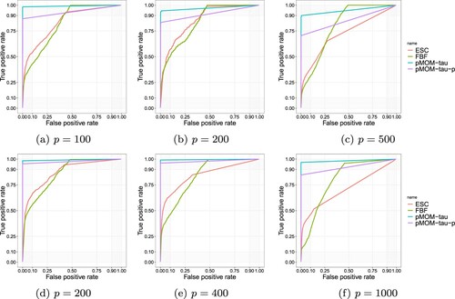
It is clear that our hierarchical Bayesian approach with pMOM Cholesky prior under two different values of τ outperforms Lasso-DAG, ESC and FBF approaches based on almost all measures. The FDR values for our Bayesian pMOM Cholesky approaches are mostly below 0.3 except when p = 1000, while the ones for the other methods are around or beyond 0.5. The TPR values for the proposed approaches are all beyond 0.6 in most cases, while the ones for the penalized likelihood approaches and other two Bayesian approaches are all below 0.55 in most scenarios. For the most comprehensive measure of MCC, our proposed Bayesian approach outperforms all the other three methods under all the cases of $(n,p)$ and two different sparsity settings. It is also worthwhile to compare the simulation performance between three different values of τ under the pMOM Cholesky prior. We can tell that the higher order of ${\tau }_p$ though could guarantee the strong model selection consistency (Theorem 4.3), compared with the constant ${\tau }_1$ and ${\tau }_2$ case, the selection performance slightly suffers from the strong penalty induced by both the pMOM prior itself and the larger ${\tau }_p$ value. The performance under $\tau =1$ and $\tau =2$ are very similar with a slightly better performance given by $\tau =1$. Hence, from a practical standpoint, one would prefer treating τ as a smaller constant (not growing with p) for better estimation accuracy.

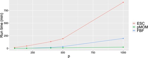
It is also meaningful to compare the computational runtime between different methods. In Figure 2, we plot the run time comparison among our pMOM Cholesky approach, ESC and FBF. We can see that the run time for pMOM is significantly lessened compared to ESC and FBF, especially under the setting where we ran each ESC-based chain for 5000 iterations, while for pMOM, we ran 10,000 iterations. The computational cost of ESC is also extremely expensive in the sense that it requires not only additional run time, but also larger memory (more than 30 GB when $p>900$).

Figure 2. Run time comparison.

Overall, this experiment illustrates that the proposed hierarchical Bayesian approach with our pMOM Cholesky prior can be used for a broad yet computationally feasible model search, and at the same time can lead to a much more significant improvement in model selection performance for estimating the sparsity pattern of the Cholesky factor and the underlying DAG.

7. Results for hyper-pMOM Cholesky prior

In the generalized linear regression setting, Wu (2016) proposes a fully Bayesian approach with the hyper-pMOM prior where an appropriate Inverse-Gamma prior $\text{Inverse-Gamma}({\lambda }_1,{\lambda }_2)$ is placed on the parameter τ in the pMOM prior. Following the nomenclature in Wu (2016), we refer to the following mixture of priors as the hyper-pMOM Cholesky prior, (13) $\begin{array}{rl}{L}_{Z_j,j}\mid d_j,Z_j& \stackrel{\mathrm{i}\mathrm{n}\mathrm{d}}{\sim }\text{pMOM Cholesky},1\le j<p,\end{array}$(13) (14) $\begin{array}{rl}{d}_j& \stackrel{\mathrm{i}\mathrm{n}\mathrm{d}}{\sim }\text{Inverse-Gamma}({\alpha }_1,{\alpha }_2),1\le j\le p,\end{array}$(14) (15) $\begin{array}{rl}\tau & \sim \text{Inverse-Gamma}({\lambda }_1,{\lambda }_2),\end{array}$(15) where ${\lambda }_1$ and ${\lambda }_2$ are positive constants.

Note that as indicated in Wu (2016) and Cao et al. (2020), compared to the pMOM density in (2(2) $\begin{array}{rl}& m_p\left(2\pi {)}^{-\frac{p}{2}}\right(\tau {\sigma }^2{)}^{-rp-\frac{p}{2}}|A_p{|}^{\frac{1}{2}}\\ & \times \exp \left(-\frac{{\text{β}}_p^{\mathrm{T}}{A}_p{\text{β}}_p}{2\tau {\sigma }^2}\right)\prod _{i=1}^p{\text{β}}_i^{2r}.\end{array}$(2) ) with given τ, the marginal hyper-pMOM now possesses thicker tails that induce prior dependence. In addition, this type of mixture of priors could achieve better model selection performance especially for small samples (Liang et al., 2008).

By (13(13) $\begin{array}{rl}{L}_{Z_j,j}\mid d_j,Z_j& \stackrel{\mathrm{i}\mathrm{n}\mathrm{d}}{\sim }\text{pMOM Cholesky},1\le j<p,\end{array}$(13) )–(15(15) $\begin{array}{rl}\tau & \sim \text{Inverse-Gamma}({\lambda }_1,{\lambda }_2),\end{array}$(15) ), under the hyper-pMOM Cholesky prior, the resulting posterior probability for $Z_j$ is given by, (16) $\begin{array}{rl}& \pi \left(Z_j|\mathit{Y}\right)\\ & \propto \pi \left(Z_j\right)m_{|Z_j|}|A_{Z_j,Z_j}{|}^{\frac{1}{2}}\\ & \times {\int }_0^{\mathrm{\infty }}{\int }_0^{\mathrm{\infty }}{\tau }^{-r|Z_j|-\frac{|Z_j|}{2}-({\lambda }_1+1)}{\mathrm{e}}^{-\frac{{\lambda }_2}{\tau }}\frac{1}{|n{\tilde{S}}_{Z_j,Z_j}{|}^{\frac{1}{2}}}\\ & \times d_j^{-\left(\frac{n}{2}+(r-\frac{1}{2})|Z_j|+{\alpha }_1+1\right)}\\ & \times \exp \left(-\frac{n{\tilde{S}}_{j|Z_j}+2{\alpha }_2}{2d_j}\right)E_{|Z_j|}\left(\prod _{i\in Z_j}{L}_{ij}^{2r}\right)\mathrm{d}{d}_j\mathrm{d}\tau ,\end{array}$(16) where ${\tilde{S}}_{Z_j,Z_j}=S_{Z_j,Z_j}+\frac{A_{Z_j,Z_j}}{n\tau }$, ${\tilde{S}}_{j|Z_j}={\tilde{S}}_{jj}-({\tilde{S}}_{Z_j,j}{)}^{\mathrm{T}}\times ({\tilde{S}}_{Z_j,Z_j}{)}^{-1}{\tilde{S}}_{Z_j,j},$ and $E_{|Z_j|}(.)$ denotes the expectation with respect to a multivariate normal distribution with mean $-({\tilde{S}}_{Z_j,Z_j}{)}^{-1}{\tilde{S}}_{Z_j,j}$, and covariance matrix $d_j(n{\tilde{S}}_{Z_j,Z_j}{)}^{-1}$. Since these posterior probabilities are still not available in closed, we have the following lemma that provides the upper bound for the Bayes factor under the following assumption.

Assumption 5c

The hyperparameters $A_p$, ${\alpha }_1,{\alpha }_2,{\lambda }_1,{\lambda }_2$ in (13(13) $\begin{array}{rl}{L}_{Z_j,j}\mid d_j,Z_j& \stackrel{\mathrm{i}\mathrm{n}\mathrm{d}}{\sim }\text{pMOM Cholesky},1\le j<p,\end{array}$(13) )–(15(15) $\begin{array}{rl}\tau & \sim \text{Inverse-Gamma}({\lambda }_1,{\lambda }_2),\end{array}$(15) ) satisfy $0<a_1<{\mathrm{e}\mathrm{i}\mathrm{g}}_1\left(A_p\right)\le {\mathrm{e}\mathrm{i}\mathrm{g}}_2\left(A_p\right)\le \dots \le {\mathrm{e}\mathrm{i}\mathrm{g}}_p\left(A_p\right)<a_2<\mathrm{\infty }$ and $0<{\alpha }_1,{\alpha }_2,{\lambda }_1,{\lambda }_2<a_2$. Here $a_1,a_2$ are constants not depending on n.

Lemma 7.1

Under Assumption 1–5c, for each $1\le j<p$, the Bayes factor between any ‘non-true’ model $Z_j$ and the true model ${Z_0}_j$ under the hyper-pMOM Cholesky prior will be bound above by, (17) $\begin{array}{rl}& \frac{\pi \left(\mathit{Y}|Z_j\right)}{\pi \left(\mathit{Y}|{Z_0}_j\right)}\\ & \le (M{n}^{1/2}{)}^{-(|Z_j|-|{Z_0}_j|)}\\ & \times \frac{(|Z_j{|}^{-1}V{)}^{r|Z_j|}}{(\frac{s}{2}{)}^{2r|{Z_0}_j|}}\frac{\mathrm{\Gamma }\left(\frac{n}{2}+\left(r-\frac{1}{2}\right)|Z_j|+{\alpha }_1\right)}{\mathrm{\Gamma }\left(\frac{n}{2}+\left(r-\frac{1}{2}\right)|{Z_0}_j|+{\alpha }_1\right)}\\ & \times \frac{\mathrm{\Gamma }(r|Z_j|+\frac{|Z_j|}{2}+{\lambda }_1)}{\mathrm{\Gamma }(r|{Z_0}_j|+\frac{|{Z_0}_j|}{2}+{\lambda }_1)}\\ & \times \frac{(n{\tilde{S}}_{j|{Z_0}_j}/2+{\alpha }_2{)}^{\frac{n}{2}+(r-\frac{1}{2})|{Z_0}_j|+{\alpha }_1}}{(n{\tilde{S}}_{j|Z_j}/2+{\alpha }_2{)}^{\frac{n}{2}+(r-\frac{1}{2})|Z_j|+{\alpha }_1}}\\ & \times \frac{({\lambda }_2+c_3|{Z_0}_j|/n+c_4{)}^{r|{Z_0}_j|+\frac{|{Z_0}_j|}{2}+{\lambda }_1}}{({\lambda }_2-c_2|Z_j|/(2n){)}^{r|Z_j|+\frac{|Z_j|}{2}+{\lambda }_1}}\\ & +(M{n}^{1/2}{)}^{-(|Z_j|-|{Z_0}_j|)}\frac{n^{-r|Z_j|}}{{\left(\frac{s}{2}\right)}^{2r|{Z_0}_j|}}\\ & \times \frac{\mathrm{\Gamma }\left(\frac{n-|Z_j|}{2}+{\alpha }_1\right)}{\mathrm{\Gamma }\left(\frac{n}{2}+\left(r-\frac{1}{2}\right)|{Z_0}_j|+{\alpha }_1\right)}\frac{\mathrm{\Gamma }(r|Z_j|+\frac{|Z_j|}{2}+{\lambda }_1)}{\mathrm{\Gamma }(r|{Z_0}_j|+\frac{|{Z_0}_j|}{2}+{\lambda }_1)}\\ & \times \frac{(n{\tilde{S}}_{j|{Z_0}_j}/2+{\alpha }_2{)}^{\frac{n}{2}+(r-\frac{1}{2})|{Z_0}_j|+{\alpha }_1}}{(n{\tilde{S}}_{j|Z_j}/2+{\alpha }_2{)}^{\frac{n-|Z_j|}{2}+{\alpha }_1}}\\ & \times \frac{({\lambda }_2+c_3|{Z_0}_j|/n+c_4{)}^{r|{Z_0}_j|+\frac{|{Z_0}_j|}{2}+{\lambda }_1}}{({\lambda }_2-c_2|Z_j|/(2n){)}^{r|Z_j|+\frac{|Z_j|}{2}+{\lambda }_1}},\end{array}$(17) for some constants $M,c_2,c_3,c_4>0$.

The upper bound in (17(17) $\begin{array}{rl}& \frac{\pi \left(\mathit{Y}|Z_j\right)}{\pi \left(\mathit{Y}|{Z_0}_j\right)}\\ & \le (M{n}^{1/2}{)}^{-(|Z_j|-|{Z_0}_j|)}\\ & \times \frac{(|Z_j{|}^{-1}V{)}^{r|Z_j|}}{(\frac{s}{2}{)}^{2r|{Z_0}_j|}}\frac{\mathrm{\Gamma }\left(\frac{n}{2}+\left(r-\frac{1}{2}\right)|Z_j|+{\alpha }_1\right)}{\mathrm{\Gamma }\left(\frac{n}{2}+\left(r-\frac{1}{2}\right)|{Z_0}_j|+{\alpha }_1\right)}\\ & \times \frac{\mathrm{\Gamma }(r|Z_j|+\frac{|Z_j|}{2}+{\lambda }_1)}{\mathrm{\Gamma }(r|{Z_0}_j|+\frac{|{Z_0}_j|}{2}+{\lambda }_1)}\\ & \times \frac{(n{\tilde{S}}_{j|{Z_0}_j}/2+{\alpha }_2{)}^{\frac{n}{2}+(r-\frac{1}{2})|{Z_0}_j|+{\alpha }_1}}{(n{\tilde{S}}_{j|Z_j}/2+{\alpha }_2{)}^{\frac{n}{2}+(r-\frac{1}{2})|Z_j|+{\alpha }_1}}\\ & \times \frac{({\lambda }_2+c_3|{Z_0}_j|/n+c_4{)}^{r|{Z_0}_j|+\frac{|{Z_0}_j|}{2}+{\lambda }_1}}{({\lambda }_2-c_2|Z_j|/(2n){)}^{r|Z_j|+\frac{|Z_j|}{2}+{\lambda }_1}}\\ & +(M{n}^{1/2}{)}^{-(|Z_j|-|{Z_0}_j|)}\frac{n^{-r|Z_j|}}{{\left(\frac{s}{2}\right)}^{2r|{Z_0}_j|}}\\ & \times \frac{\mathrm{\Gamma }\left(\frac{n-|Z_j|}{2}+{\alpha }_1\right)}{\mathrm{\Gamma }\left(\frac{n}{2}+\left(r-\frac{1}{2}\right)|{Z_0}_j|+{\alpha }_1\right)}\frac{\mathrm{\Gamma }(r|Z_j|+\frac{|Z_j|}{2}+{\lambda }_1)}{\mathrm{\Gamma }(r|{Z_0}_j|+\frac{|{Z_0}_j|}{2}+{\lambda }_1)}\\ & \times \frac{(n{\tilde{S}}_{j|{Z_0}_j}/2+{\alpha }_2{)}^{\frac{n}{2}+(r-\frac{1}{2})|{Z_0}_j|+{\alpha }_1}}{(n{\tilde{S}}_{j|Z_j}/2+{\alpha }_2{)}^{\frac{n-|Z_j|}{2}+{\alpha }_1}}\\ & \times \frac{({\lambda }_2+c_3|{Z_0}_j|/n+c_4{)}^{r|{Z_0}_j|+\frac{|{Z_0}_j|}{2}+{\lambda }_1}}{({\lambda }_2-c_2|Z_j|/(2n){)}^{r|Z_j|+\frac{|Z_j|}{2}+{\lambda }_1}},\end{array}$(17) ) can be used to show the posterior ratio consistency illustrated in the following theorem.

Theorem 7.2

Under Assumptions 1–5c, if we assume ${\lambda }_1$ and ${\lambda }_2$ are some fixed positive constants, the following holds under the hyper-pMOM Cholesky prior: for all $1\le j<p$, $\begin{array}{rl}& \underset{Z_j\ne {Z_0}_j}{max}\frac{\pi \left(Z_j|\mathit{Y}\right)}{\pi \left({Z_0}_j|\mathit{Y}\right)}\stackrel{P_{{\mathrm{\Omega }}_0}}{⟶}0,\text{and}{P}_{{\mathrm{\Omega }}_0}({\hat{Z}}_j={Z_0}_j)\to 1,\\ & \text{as }n\to \mathrm{\infty }.\end{array}$

In order to achieve strong model selection consistency, we need the following assumption on the hyperparameter ${\lambda }_2$ instead of Assumption 5c.

Assumption 5d

The hyperparameters $A_p$, ${\alpha }_1,{\alpha }_2,{\lambda }_1,{\lambda }_2$ in (13(13) $\begin{array}{rl}{L}_{Z_j,j}\mid d_j,Z_j& \stackrel{\mathrm{i}\mathrm{n}\mathrm{d}}{\sim }\text{pMOM Cholesky},1\le j<p,\end{array}$(13) )–(15(15) $\begin{array}{rl}\tau & \sim \text{Inverse-Gamma}({\lambda }_1,{\lambda }_2),\end{array}$(15) ) satisfy $0<a_1<{\mathrm{e}\mathrm{i}\mathrm{g}}_1\left(A_p\right)\le {\mathrm{e}\mathrm{i}\mathrm{g}}_2\left(A_p\right)\le \dots \le {\mathrm{e}\mathrm{i}\mathrm{g}}_p\left(A_p\right)<a_2<\mathrm{\infty }$, $0<{\alpha }_1,{\alpha }_2,{\lambda }_1<a_2$ and ${\lambda }_2\sim p^{2\kappa /(r+1/2)}$, for some $\kappa >1$. Here $a_1,a_2$ are constants not depending on n.

The next theorem establishes the strong selection consistency under the hyper-pMOM Cholesky prior. See proofs for Theorems 7.2 and 7.3 in the supplement.

Theorem 7.3

Under Assumptions 1–5d, for the hyper-pMOM Cholesky prior, the following holds: for all $1\le j<p$, $\pi \left({Z_0}_j|\mathit{Y}\right)\stackrel{P_{{\mathrm{\Omega }}_0}}{⟶}1,\text{as }n\to \mathrm{\infty }.$

Note that for the hyper-pMOM Cholesky prior with the extra layer of prior on τ, the Newton-type algorithm used for optimizing the likelihood could be quite time consuming, and the estimation accuracy will be compromised, especially when the size of the model and the dimension p are large. Therefore, from a practical standpoint, we would still prefer the pMOM Cholesky prior for carrying out the model selection.

8. Discussion

In this paper, we investigate the theoretical consistency properties for the high-dimensional sparse DAG models based on proper non-local priors, namely the pMOM Cholesky and the hyper-pMOM Cholesky priors. We establish both posterior ratio consistency and strong model selection consistency under comparably more general conditions than those in the existing literature. In addition, by putting a uniform-like prior over the space of sparsity pattern for Cholesky factors, we avoid the potential issues of the model being stuck in rather sparse space caused by the priors over the graph space aiming to penalize larger models like the Erdos–Renyi prior, the beta-mixture prior or the multiplicative prior. Also, through simulation studies where we implement an efficient parallel MCMC algorithm for exploring the sparsity pattern of each column of L, we demonstrate that the models studied in this paper can outperform existing state-of-the-art methods including both penalized likelihood and Bayesian approaches in different settings.

Acknowledgments

We would like to thank the Editor, the Associate Editor and the reviewer for their insightful comments which have led to improvements of an earlier version of this paper.

Additional information

Funding

This work was supported by Simons Foundation's collaboration grant (No. 635213).

References

- Altamore, D., Consonni, G., & La Rocca, L. (2013). Objective Bayesian search of gaussian directed acyclic graphical models for ordered variables with non-local priors. Biometrics, 69(2), 478–487. https://doi.org/https://doi.org/10.1111/biom.v69.2
- Banerjee, S., & Ghosal, S. (2014). Posterior convergence rates for estimating large precision matrices using graphical models. Electronic Journal of Statistics, 8(2), 2111–2137. https://doi.org/https://doi.org/10.1214/14-EJS945
- Banerjee, S., & Ghosal, S. (2015). Bayesian structure learning in graphical models. Journal of Multivariate Analysis, 136, 147–162. https://doi.org/https://doi.org/10.1016/j.jmva.2015.01.015
- Ben-David, E., Li, T., Massam, H., & Rajaratnam, B. (2016). High dimensional Bayesian inference for Gaussian directed acyclic graph models (Tech. Rep.). http://arxiv.org/abs/1109.4371
- Bhadra, A., & Mallick, B. (2013). Joint high-dimensional Bayesian variable and covariance selection with an application to eQTL analysis. Biometrics, 69(2), 447–457. https://doi.org/https://doi.org/10.1111/biom.v69.2
- Bickel, P. J., & Levina, E. (2008). Regularized estimation of large covariance matrices. Annals of Statistics, 36(1), 199–227. https://doi.org/https://doi.org/10.1214/009053607000000758
- Cai, T., Liu, W., & Luo, X. (2011). A constrained ℓ1 minimization approach to sparse precision matrix estimation. Journal of the American Statistical Association, 106(494), 594–607. https://doi.org/https://doi.org/10.1198/jasa.2011.tm10155
- Cao, X., Khare, K., & Ghosh, M. (2019). Posterior graph selection and estimation consistency for high-dimensional Bayesian DAG models. Annals of Statistics, 47(1), 319–348. https://doi.org/https://doi.org/10.1214/18-AOS1689
- Cao, X., Khare, K., & Ghosh, M. (2020). High-dimensional posterior consistency for hierarchical non-local priors in regression. Bayesian Analysis, 15(1), 241–262. https://doi.org/https://doi.org/10.1214/19-BA1154
- Carvalho, C. M., & Scott, J. G. (2009). Objective Bayesian model selection in Gaussian graphical models. Biometrika, 96(3), 497–512. https://doi.org/https://doi.org/10.1093/biomet/asp017
- El Karoui, N. (2008). Spectrum estimation for large dimensional covariance matrices using random matrix theory. Annals of Statistics, 36(6), 2757–2790. https://doi.org/https://doi.org/10.1214/07-AOS581
- Huang, J., Liu, N., Pourahmadi, M., & Liu, L. (2006). Covariance selection and estimation via penalised normal likelihood. Biometrika, 93(1), 85–98. https://doi.org/https://doi.org/10.1093/biomet/93.1.85
- Johnson, V., & Rossell, D. (2010). On the use of non-local prior densities in Bayesian hvoothesis tests hypothesis. Journal of the Royal Statistical Society: Series B (Statistical Methodology), 72(2), 143–170. https://doi.org/https://doi.org/10.1111/rssb.2010.72.issue-2
- Johnson, V., & Rossell, D. (2012). Bayesian model selection in high-dimensional settings. Journal of the American Statistical Association, 107(498), 649–660. https://doi.org/https://doi.org/10.1080/01621459.2012.682536
- Khare, K., Oh, S., Rahman, S., & Rajaratnam, B. (2017). A convex framework for high-dimensional sparse Cholesky based covariance estimation in Gaussian DAG models [Preprint, Department of Statisics, University of Florida].
- Lee, K., Lee, J., & Lin, L. (2019). Minimax posterior convergence rates and model selection consistency in high-dimensional DAG models based on sparse Cholesky factors. Annals of Statistics, 47(6), 3413–3437. https://doi.org/https://doi.org/10.1214/18-AOS1783
- Liang, F., Paulo, R., Molina, G., Clyde, A. M., & Berger, O. J. (2008). Mixtures of g priors for Bayesian variable selection. Journal of the American Statistical Association, 103(481), 410–423. https://doi.org/https://doi.org/10.1198/016214507000001337
- Narisetty, N., & He, X. (2014). Bayesian variable selection with shrinking and diffusing priors. Annals of Statistics, 42(2), 789–817. https://doi.org/https://doi.org/10.1214/14-AOS1207
- Niu, Y., Pati, D., & Mallick, B. (2019). Bayesian graph selection consistency under model misspecification. arxiv:1901.04134
- Pourahmadi, M. (2007). Cholesky decompositions and estimation of a covariance matrix: Orthogonality of variance–correlation parameters. Biometrika, 94(4), 1006–1013. https://doi.org/https://doi.org/10.1093/biomet/asm073
- Rossell, D., Telesca, D., & Johnson, V. E. (2013). High-dimensional Bayesian classifiers using non-local priors. In Statistical models for data analysis. Springer.
- Scott, J. G., & Carvalho, C. M. (2008). Feature-inclusion stochastic search for gaussian graphical models. Journal of Computational and Graphical Statistics, 17(4), 790–808. https://doi.org/https://doi.org/10.1198/106186008X382683
- Shin, M., Bhattacharya, A., & Johnson, V. (2018). Scalable Bayesian variable selection using nonlocal prior densities in ultrahigh-dimensional settings. Statistica Sinica, 28(2), 1053–1078. https://doi.org/https://doi.org/10.5705/ss.202016.0167
- Shojaie, A., & Michailidis, G. (2010). Penalized likelihood methods for estimation of sparse high-dimensional directed acyclic graphs. Biometrika, 97(3), 519–538. https://doi.org/https://doi.org/10.1093/biomet/asq038
- Tan, L. S. L., Jasra, A., De Iorio, M., & Ebbels, T. M. D. (2017). Bayesian inference for multiple gaussian graphical models with application to metabolic association networks. The Annals of Applied Statistics, 11(4), 2222–2251. https://doi.org/https://doi.org/10.1214/17-AOAS1076
- van de Geer, S., & Bühlmann, P. (2013). ℓ0-penalized maximum likelihood for sparse directed acyclic graphs. The Annals of Statistics, 41(2), 536–567. https://doi.org/https://doi.org/10.1214/13-AOS1085
- Wu, H.-H. (2016). Nonlocal priors for Bayesian variable selection in generalized linear models and generalized linear mixed models and their applications in biology data [PhD thesis, University of Missouri].
- Xiang, R., Khare, K., & Ghosh, M. (2015). High dimensional posterior convergence rates for decomposable graphical models. Electronic Journal of Statistics, 9(2), 2828–2854. https://doi.org/https://doi.org/10.1214/15-EJS1084
- Yang, Y., Wainwright, M. J., & Jordan, M. I. (2016). On the computational complexity of high-dimensional Bayesian variable selection. Annals of Statistics, 44(6), 2497–2532. https://doi.org/https://doi.org/10.1214/15-AOS1417
- Yu, G., & Bien, J. (2017). Learning local dependence in ordered data. Journal of Machine Learning Research, 18(42), 1–60.
- Zhang, T., & Zou, H. (2014). Sparse precision matrix estimation via lasso penalized D-trace loss. Biometrika, 101(1), 103–120. https://doi.org/https://doi.org/10.1093/biomet/ast059