Asymptotic properties of a nonparametric conditional density estimator in the local linear estimation for functional data via a functional single-index model

Abstract

This paper deals with the conditional density estimator of a real response variable given a functional random variable (i.e., takes values in an infinite-dimensional space). Specifically, we focus on the functional index model, and this approach represents a good compromise between nonparametric and parametric models. Then we give under general conditions and when the variables are independent, the quadratic error and asymptotic normality of estimator by local linear method, based on the single-index structure. Finally, we complete these theoretical advances by some simulation studies showing both the practical result of the local linear method and the good behaviour for finite sample sizes of the estimator and of the Monte Carlo methods to create functional pseudo-confidence area.

Keywords:

• Mean squared error
• single functional index
• conditional density function
• nonparametric estimation
• local linear estimation
• asymptotic normality
• functional data

1. Introduction

The nonparametric estimation of the conditional density function plays a crucial role in statistical analysis. This subject can be approached from multiple perspectives depending on the complexity of the problem. Many techniques were studied in the literature to treat these various situations but all treat only real or multidimensional explanatory random variables.

Focusing on functional data for the kernel-type, the first results on the nonparametric estimate of this model were got by Ferraty and Vieu (2006). They have studied the almost complete convergence the estimator of the conditional density and its derivates. Laksaci (2007) studied quadratic error of this estimator, and we return to Ferraty et al. (2010) which established the uniform almost complete convergence of this model always.

Now, we show a few results on the local linear smoothing for functional data, actually these results have been considered by many authors. Baìllo and Grané (2009) first proposed a local linear smoothing of the regression estimator in a Hilbert space, and coming after them Barrientos-Marin et al. (2010) developed this method of local linear estimation of the regression in the semi-metric space for independent and identically distributed. Demongeot et al. (2013, 2014), has used this method to estimate conditional distribution and density function. In the case of spatial data (Laksaci et al., 2013) they established pointwise almost complete convergence rates.

Furthermore, the functional index model plays a major role in statistics. The interest of this approach comes from its use to reduce the dimension of the data by projection in fractal space. The literature on this topic is closely limited, the first work which was interested in the single-index model on the nonparametric estimation is Ferraty et al. (2003) which stated for i.i.d. variables and obtained the almost complete convergence under some conditions. Based on the cross-validation procedure, Ait Saidi et al. (2008) proposed an estimator of this parameter, where the functional single-index is unknown. Recently, Attaoui et al. (2011) considered the nonparametric estimation of the conditional density in the single functional model. They established its pointwise and uniform almost complete convergence (a.co.) rates. In the same topic, Attaoui and Ling (2016) proved the asymptotic results of a nonparametric conditional cumulative distribution estimator for time series data. More recently, Tabti and Ait Saidi (2018) obtained the almost complete convergence and the uniform almost complete convergence of a kernel estimator of the hazard function with quasi-association condition when the observations are linked with functional single-index structure.

In this paper, we focus on the local linear estimation with the single-index structure to compute under some conditions, the quadratic error of the conditional density function estimator. In practice, this study has great importance, because, it permits to construct a prediction method based on the maximum risk estimation with a single functional index.

In Section 2, We introduce the estimator of our model in the single functional index. In Section 3, we introduce assumptions and asymptotic properties are given. Simulations are given in Section 4. Finally, Section 5 is devoted to the proofs of the results.

2. The model

Let $\left\{\right(X_i,Y_i),1\le i\le n\}$ be n random variables, independent and identically distributed as the random pair $(X,Y)$ with values in $\mathcal{H}\times \mathbb{R},$ where $\mathcal{H}$ is a separable real Hilbert space with the norm $\parallel .\parallel$ generated by an inner product $〈.,.〉$. We consider the semi-metric $d_{\theta }$ associated to the single-index $\theta \in \mathcal{H}$ defined by $d_{\theta }(x_1,x_2):=\mid 〈x_1-x_2,\theta 〉\mid ,\mathrm{\forall }{x}_1,x_2\in \mathcal{H}$. Assume that the explanation of Y given X is done through a fixed functional index θ in $\mathcal{H}$. In the sense, there exists a θ in $\mathcal{H}$ (unique up to a scale normalization factor) such that: $\mathbb{E}\left[Y|X\right]=\mathbb{E}[Y|〈\theta ,X〉]$. The conditional density of Y given X = x denoted by $f_{\theta }(.|x)$ exists and is given by $f_{\theta }\left(y|x\right):=f(y|〈x,\theta 〉),\mathrm{\forall }y\in \mathbb{R}.$ In the following, we denote by $f(\theta ,.,x)$, the conditional density of Y given $〈x,\theta 〉$ and we define the local linear estimator for single-index structure $\hat{f}(\theta ,.,x)$ of $f(\theta ,.,x)$ by $\begin{array}{rl}\hat{f}(\theta ,y,x)& =\frac{\sum _{1\le i,j\le n}{W}_{ij}(\theta ,x)H\left({h_H}^{-1}\right(y-Y_j\left)\right)}{h_H\sum _{1\le i,j\le n}{W}_{ij}(\theta ,x)}\\ & =\frac{\sum _{1\le j\le n}{\mathrm{\Omega }}_j{K}_j{H}_j}{h_H\sum _{1\le j\le n}{\mathrm{\Omega }}_j{K}_j},\end{array}$with $\begin{array}{rl}{W}_{ij}(\theta ,x)& ={\text{β}}_{\theta }(X_i,x)({\text{β}}_{\theta }(X_i,x)-{\text{β}}_{\theta }(X_j,x))\\ & \times K\left(h_K^{-1}{d}_{\theta }\right(x,X_i\left)\right)K\left(h_K^{-1}{d}_{\theta }\right(x,X_j\left)\right),\end{array}$and ${\mathrm{\Omega }}_j{K}_j=\sum _{i=1}^n{W}_{ij}$ with ${\text{β}}_{\theta }(X_i,x)$ is a known bi-functional operator from ${\mathcal{H}}^2$ into $\mathbb{R}$ where K and H are kernel functions and $h_K:=h_{n,K}$ (resp. $h_H:=h_{n,H}$) is a sequence that decreases to zero as n goes to infinity.

3. Assumptions and mains results

Throughout the paper, we will denote by C, $C^{\mathrm{\prime }}$ and $C_{\theta ,x}$ some strictly positive generic constants and $K_i(\theta ,x):=K\left(h_K^{-1}{d}_{\theta }\right(x,X_i\left)\right),\mathrm{\forall }x\in \mathcal{H},i=1,\dots ,n$, $H_j:=H\left({h_H}^{-1}\right(y-Y_j\left)\right),\mathrm{\forall }y\in \mathbb{R},j=1,\dots ,n.$, ${\text{β}}_{\theta ,i}:={\text{β}}_{\theta }(X_i,x),$ $W_{ij}(\theta ,x):=W_{\theta ,ij}$ and we will use the notation $B_{\theta }(x,h_K):=\{x_1\in \mathcal{H}:0<|〈x-x_1,\theta 〉|<h_K\}$, the ball centred at x with radius $h_K$. Moreover, to find the results in our paper we denote ${\psi }_l(.,y):=\frac{{\mathrm{\partial }}^{l}f(.,y,.)}{\mathrm{\partial }{y}^l}$, for any $l\in \{0,2\}$

${\mathrm{\Phi }}_l\left(s\right)=\mathbb{E}\left[{\psi }_l\right(X,y)-{\psi }_l(x,y\left)|d_{\theta }\right(x,X)=s]$.

In order to study our asymptotic results, we need the following assumptions:

(H1)	$\mathbb{P}(X\in B_{\theta }(x,h_K\left)\right)=:{\varphi }_{\theta ,x}\left(h_K\right)>0$, and assume that there exists a function ${\chi }_{\theta ,x}(\cdot )$ such that $\underset{h_K\to 0}{lim}\frac{{\varphi }_{\theta ,x}(s{h}_K,h_K)}{{\varphi }_{\theta ,x}\left(h_K\right)}={\chi }_{\theta ,x}\left(s\right),\mathrm{\forall }s\in [-1,1].$
(H2)	For any $l\in \{0,2\}$, the quantities ${\mathrm{\Phi }}_l^{\mathrm{\prime }}\left(0\right)$ and ${\mathrm{\Phi }}_l^{\mathrm{\prime }\mathrm{\prime }}\left(0\right)$ exist, where ${\mathrm{\Phi }}_l^{\mathrm{\prime }}$ (resp.${\mathrm{\Phi }}_l^{\mathrm{\prime }\mathrm{\prime }}$) denotes the first (resp. the second) derivative of ${\mathrm{\Phi }}_l$.
(H3)	The bi-functional ${\text{β}}_{\theta }(.,.)$ satisfies $\begin{array}{r}\begin{array}{cc}& \mathrm{\forall }{x}^{\mathrm{\prime }}\in \mathcal{F},C_1{d}_{\theta }(x,x^{\mathrm{\prime }})\le |{\text{β}}_{\theta }(x,x^{\mathrm{\prime }})|\\ & \le C_2{d}_{\theta }(x,x^{\mathrm{\prime }}),\text{ where }{C}_1>0,C_2>0,\\ & \underset{u\in B(x,r)}{sup}|{\text{β}}_{\theta }(u,x)-d_{\theta }(x,u)|=o\left(r\right),\\ & h_K{\int }_{B(x,h_K)}{\text{β}}_{\theta }(u,x)\mathrm{d}P\left(u\right)\\ & =o\left({\int }_{B(x,h_K)}{\text{β}}_{\theta }^2\right(u,x\left)\mathrm{d}P\right(u\left)\right),\end{array}\end{array}$where $B_{\theta }(x,r)=\{x^{\mathrm{\prime }}\in \mathcal{H}/|d_{\theta }(x,x^{\mathrm{\prime }})\le r\}$ and $\mathrm{d}P\left(x\right)$ is the cumulative distribution of X.
(H4)	The kernel K is a positive, differentiable function and its derivative $K^{\mathrm{\prime }}$ exists and is such that there exist two constants C and $C^{\mathrm{\prime }}$ with $-\mathrm{\infty }<C<K^{\mathrm{\prime }}\left(t\right)<C^{\mathrm{\prime }}<0,\text{ for }t\in [-1,1]\text{ and }K\left(1\right)>0.$
(H5)	The kernel H is a differentiable function and bounded, such that $\begin{array}{rl}& \int H\left(t\right)\mathrm{d}t=1,\int t^{2}H\left(t\right)\mathrm{d}t<\mathrm{\infty }\mathrm{a}\mathrm{n}\mathrm{d}\\ & \int H^2\left(t\right)\mathrm{d}t<\mathrm{\infty }.\end{array}$
(H6)	The bandwidths $h_K$,$h_H$ satisfy ${\displaystyle \underset{n\to \mathrm{\infty }}{lim}{h}_K=0,\underset{n\to \mathrm{\infty }}{lim}{h}_H=0\text{ and }\underset{n\to \mathrm{\infty }}{lim}n{h}_H{\varphi }_{\theta ,x}\left(h_K\right)=\mathrm{\infty },}$ ${\displaystyle \underset{n\to \mathrm{\infty }}{lim}n{h}_H^5{\varphi }_{\theta ,x}\left(h_K\right)=0}$ and ${\displaystyle \underset{n\to \mathrm{\infty }}{lim}n{h}_H{h}_K^2{\varphi }_{\theta ,x}\left(h_K\right)=0.}$

Comments on assumptions: Notice that, (H1) and (H2) are a simple adaptation of the conditions in Ferraty et al. (2007) on the regression operator, when we replace the semi-metric by some bi-functional $d_{\theta }$. The second part of the condition (H3) is unrestrictive and is verified, for instance, if $d_{\theta }(\cdot ,\cdot )={\text{β}}_{\theta }(\cdot ,\cdot )$; moreover $\underset{d_{\theta }(x,u)\to 0}{lim}|\frac{{\text{β}}_{\theta }(u,x)}{d_{\theta }(x,u)}-1|=0.$Assumptions (H4)–(H6) are classical in this context of quadratic errors and asymptotic normality in functional statistic.

3.1. Mean square convergence

In this part, we are going to show the asymptotic results of quadratic-mean convergence.

Theorem 3.1

Under assumptions (H1)–(H6), we obtain $\begin{array}{rl}& \mathbb{E}{\left[\hat{f}\right(\theta ,y,x)-f(\theta ,y,x\left)\right]}^2\\ & =B_H^2(\theta ,x,y)h_H^4+B_K^2(\theta ,x,y)h_K^2+\frac{V_{HK}(\theta ,x,y)}{n{h}_H{\varphi }_{\theta ,x}\left(h_K\right)}\\ & +o\left(h_H^4\right)+o\left(h_K^2\right)+o\left(\frac{1}{n{h}_H{\varphi }_{\theta ,x}\left(h_K\right)}\right),\end{array}$where $\begin{array}{rl}{B}_H(\theta ,x,y)& =\frac{1}{2}\frac{{\mathrm{\partial }}^{2}f(\theta ,y,x)}{\mathrm{\partial }{y}^2}\int t^{2}H\left(t\right)\mathrm{d}t,\\ B_K(\theta ,x,y)& ={\mathrm{\Phi }}_0^{\mathrm{\prime }}\left(0\right)\frac{M_0}{M_1}{h}_K,\end{array}$and $V_{HK}(\theta ,x,y)=\frac{M_{2}f(\theta ,y,x)}{M_1^2}(\int H^2(t\left)\mathrm{d}t\right),$with $\begin{array}{rl}{M}_0& =K\left(1\right)-{\int }_0^{1}s{K}^{\mathrm{\prime }}\left(s\right){\chi }_{\theta ,x}\left(s\right)\mathrm{d}s\text{and}\\ M_j& =K^j\left(1\right)-{\int }_0^1\left(K^j{)}^{\mathrm{\prime }}\right(s\left){\chi }_{\theta ,x}\right(s)\mathrm{d}s\text{for}j=1,2.\end{array}$We set $\hat{f}(\theta ,y,x)=\frac{{\hat{f}}_N(\theta ,y,x)}{{\hat{f}}_D(\theta ,x)},$where $\begin{array}{rl}{\hat{f}}_N(\theta ,y,x)& =\frac{1}{n(n-1)h_H\mathbb{E}\left[W_{12}\right(\theta ,x\left)\right]}\\ & \times \sum _{1\le i\ne j\le n}{W}_{ij}(\theta ,x)H\left(h_H^{-1}\right(y-Y_j\left)\right),\end{array}$and ${\hat{f}}_D(\theta ,x)=\frac{1}{n(n-1)\mathbb{E}\left[W_{12}\right(\theta ,x\left)\right]}\sum _{1\le i\ne j\le n}{W}_{ij}(\theta ,x).$

The following lemmas will be useful for proof of Theorem 3.1.

Lemma 3.2

Under the assumptions of Theorem 3.1, we obtain $\begin{array}{rl}& \mathbb{E}\left[{\hat{f}}_N\right(\theta ,y,x\left)\right]-f(\theta ,y,x)\\ & =B_H(\theta ,x,y)h_H^2+B_K(\theta ,x,y)h_K+o\left(h_H^2\right)+o\left(h_K\right).\end{array}$

Lemma 3.3

Under the assumptions of Theorem 3.1, we obtain $Var\left[{\hat{f}}_N\right(\theta ,y,x\left)\right]=\frac{V_{HK}(\theta ,x,y)}{n{h}_H{\varphi }_{\theta ,x}\left(h_K\right)}+o\left(\frac{1}{n{h}_H{\varphi }_{\theta ,x}\left(h_k\right)}\right).$

Lemma 3.4

Under the assumptions of Theorem 3.1, we get $Cov\left({\hat{f}}_N\right(\theta ,y,x),{\hat{f}}_D(\theta ,x\left)\right)=O\left(\frac{1}{n{\varphi }_{\theta ,x}\left(h_K\right)}\right).$

Lemma 3.5

Under the assumptions of Theorem 3.1, we get $Var\left[{\hat{f}}_D\right(\theta ,x\left)\right]=O\left(\frac{1}{n{\varphi }_{\theta ,x}\left(h_K\right)}\right).$

3.2. Asymptotic normality

This section contains results on the asymptotic normality of $\hat{f}(\theta ,y,x).$ Before announcing our main results, we introduce the quantity $N(a,b)$, which will appear in the bias and variance dominant terms: $\begin{array}{rl}N(a,b)& =K^a\left(1\right)-{\int }_{-1}^1\left(u^b{K}^a\right(u\left){)}^{\mathrm{\prime }}{\chi }_x\right(u)\mathrm{d}u\\ & \text{for all }a>0\text{ and }b=2,4\end{array}$Then, we have the following theorem

Theorem 3.6

Under assumptions (H1)–(H6), we obtain (1) $\begin{array}{rl}& \sqrt{n{h}_H{\varphi }_{\theta ,x}\left(h_K\right)}\left(\hat{f}\right(\theta ,y,x)-f(\theta ,y,x)-{\mathbb{B}}_n(\theta ,x,y\left)\right)\\ & \stackrel{D}{\to }\mathcal{N}(0,V_{HK}(\theta ,x,y\left)\right)\end{array}$(1) where (2) $V_{HK}(\theta ,x,y)=\frac{M_2}{M_1^2}f(\theta ,y,x)(\int H^2(t\left)\mathrm{d}t\right)$(2) and (3) ${\mathbb{B}}_n(\theta ,x,y)=\frac{\mathbb{E}\left({\hat{f}}_N\right(\theta ,y,x\left)\right(y\left)\right)}{\mathbb{E}\left({\hat{f}}_D\right(\theta ,x\left)\right)}-f(\theta ,y,x)$(3) with $\stackrel{D}{\to }$ denoting the convergence in distribution.

Proof

Proof of Theorem 3.6

Inspired by the decomposition given in Masry (2005), we set $\begin{array}{rl}& \hat{f}(\theta ,y,x)-f(\theta ,y,x)-{\mathbb{B}}_n(\theta ,x,y)\\ & =\frac{{\hat{f}}_N(\theta ,y,x)-f(\theta ,y,x){\hat{f}}_D(\theta ,x)-{\hat{f}}_D(\theta ,x){\mathbb{B}}_n(\theta ,x,y)}{{\hat{f}}_D(\theta ,x)}.\end{array}$If we denote (4) $\begin{array}{rl}& Q_n(\theta ,x,y)\\ & ={\hat{f}}_N(\theta ,y,x)-f(\theta ,y,x){\hat{f}}_D(\theta ,x)\\ & -\mathbb{E}\left({\hat{f}}_N\right(\theta ,y,x)-f(\theta ,y,x\left){\hat{f}}_D\right(\theta ,x)\\ & ={\hat{f}}_N(\theta ,y,x)-f(\theta ,y,x){\hat{f}}_D(\theta ,x)-{\mathbb{B}}_n(\theta ,x,y),\end{array}$(4) since $\begin{array}{rl}& {\hat{f}}_N(\theta ,y,x)-f(\theta ,y,x){\hat{f}}_D(\theta ,x)\\ & =Q_n(\theta ,x,y)+{\mathbb{B}}_n(\theta ,x,y),\end{array}$then the proof of this theorem will be completed from the following expression (5) $\begin{array}{rl}& \hat{f}(\theta ,y,x)-f(\theta ,y,x)-{\mathbb{B}}_n(\theta ,x,y)\\ & =\frac{Q_n(\theta ,x,y)-{\mathbb{B}}_n(\theta ,x,y)\left({\hat{f}}_D\right(\theta ,x)-\mathbb{E}({\hat{f}}_D(\theta ,x)\left)\right)}{{\hat{f}}_D(\theta ,x)}\end{array}$(5) and the following auxiliary results which play a main role and for which proofs are given in the appendix.

Lemma 3.7

Under assumptions (H1)–(H5), we have ${\hat{f}}_D(\theta ,x)\stackrel{P}{\to }\mathbb{E}\left({\hat{f}}_D\right(\theta ,x\left)\right)=1,$where $\stackrel{P}{\to }$ denotes the convergence in probability.

So Lemma 3.7 implies that ${\hat{f}}_D(\theta ,x)\to 1$. Moreover, ${\mathbb{B}}_n(\theta ,x,y)=o\left(1\right)$ as $n\to \mathrm{\infty }$ because of the continuity of $f(\theta ,y,x)$. Then, we obtain that $\begin{array}{rl}& \hat{f}(\theta ,y,x)-f(\theta ,y,x)-{\mathbb{B}}_n(\theta ,x,y)\\ & =\frac{Q_n(\theta ,x,y)}{{\hat{f}}_D(\theta ,x)}(1+o_p(1\left)\right).\end{array}$

Lemma 3.8

Under assumptions (H1)–(H5), we have (6) $\sqrt{n{h}_H{\varphi }_{\theta ,x}\left(h_K\right)}{Q}_n(\theta ,x,y)\stackrel{D}{\to }\mathcal{N}(0,V_{HK}(\theta ,x,y\left)\right),$(6)

where $V_{HK}(\theta ,x,y)$ is defined by (2).

Remark 3.9

As mentioned in Demongeot et al. (2013), the function ${\varphi }_{\theta ,x}\left(t\right)$ can be empirically estimated by ${\hat{\varphi }}_{\theta ,x}\left(t\right)=\frac{\mathrm{♯}\{i:|d(X_i,x)|\le t\}}{n},$where $\mathrm{♯}\left(A\right)$ denote the cardinality of the set A. So, if we take advantage of the following assumptions and (H6) $\underset{n\to +\mathrm{\infty }}{lim}\sqrt{n{h}_H{\varphi }_{\theta ,x}\left(h_K\right)}{\mathbb{B}}_n(\theta ,x,y)=0,$ we can cancel the bias term and obtain the following corollary.

Corollary 3.10

Under the assumptions of Theorem 3.6, we get $\sqrt{\frac{n{h}_H{\hat{\varphi }}_{\theta ,x}\left(h_K\right)}{V_{HK}(\theta ,x,y)}}\left(\hat{f}\right(\theta ,y,x)-f(\theta ,y,x\left)\right)\to \mathcal{N}(0,1).$

4. Simulation study

We first construct the simulation of the explanatory functional variables. In the second part, we focus on the ability of the nonparametric functional regression to predict response variables from functional predictors. Finally we illustrate the Monte-Carlo methodology to test the efficiency of the asymptotic normality results parallel the practical experiment and build functional pseudo-confidence area.

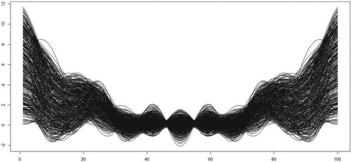
For this purpose, we consider the following process explanatory functional variables for n = 350 $\begin{array}{rl}{X}_i\left(t\right)& =\sum _{j=1}^3{V}_{ij}\cos \left(\right(3+j\left)t\right)+W_i(t-\pi {)}^2,\\ & \mathrm{\forall }t\in [0,100],\end{array}$where $V_{ij}$ and $W_i$ are n independent real random variables (r.r.v.) uniformly distributed over $[0.3;2]$ (resp. [1; 3]), and it is assumed that these curves are observed on a discretization grid of 100 points in the interval. These functional variables are represented in Figure 1.

Figure 1. The curves $X_i,i=1,\dots ,200.$

For response variables $Y_i$, we consider the following model for all $i=1,\dots n$ and $j=1,\dots 100$: $Y=r(〈{\theta }_k,X〉)+ϵ$where $r\left(U_i\right)={\int }_0^{100}\frac{1}{1-U_i^2\left(v\right)}\mathrm{d}v$ and ϵ is a centred normal variable and assumed to be independent of $(X_i{)}_i$. Then, we can get the corresponding conditional density, which is explicitly defined by $f({\theta }_k,y,x)=\frac{1}{\sqrt{2\pi }}{\mathrm{e}}^{-\frac{1}{2}{(y-r(〈{\theta }_k,x〉\left)\right)}^2}.$Our goal in this illustration is to show the usefulness of conditional density in a context of forecasting. Thus the use of optimal parameters of the conditional density is without theoretical validity.

Now, we precise the different parameters of our estimators. Indeed, first of all, it is clear that the shape of the curves allows us to use $\begin{array}{rl}& d(x_1,x_2)=\sqrt{{\int }_0^1\left(x_1\right(t)-x_2(t){)}^2\mathrm{d}t};\\ & \mathrm{\forall }{x}_1,x_2\in \mathcal{H},\text{where}\mathcal{H}\text{is a semi-metric space}.\end{array}$We choose particularly the quadratic kernels defined by $\frac{3}{2}(1-x^2){\mathbf{1}}_{[-1,1)}\text{and}K\left(1\right)>0.$In this illustration, we select the functional index ${\theta }_k$ on the set of eigenvectors of the empirical covariance operator. ${\mathrm{\Gamma }}_n\left(X\right)=\frac{1}{200}\sum _{i=1}^{200}(X_i-\overline{X}{)}^t((X_i-\overline{X})).$Indeed, we recall that the ideas of Ait Saidi et  al. (2008) can be adapted to find a method of practical selection for ${\theta }_k$. However, this adaptation in the case of the conditional density requires tools and additional preliminary results (See the discussion Attaoui et al. (2011) and Attaoui (2014)).

For this purpose, we divide our observations on two packets learning sample $(X_i,Y_i{)}_{i=1,\dots ,200}$ and test sample $(X_i,Y_i{)}_{i=201,\dots ,250}$. For the choice of smoothing parameters $h_K$ and $h_H$, we will adopt the selection criterion used by Ferraty et al.  (2006) in the case of the kernel method for which $h_K$ and $h_H$ are obtained by minimizing the next criterion (7) $\begin{array}{rl}& \frac{1}{n}\sum _{i=1}^n{W}_1\left(X_i\right)\int {\hat{f}}_{(h_K,h_H)}^{-i^2}(X_i,y)W_2\left(y\right)\mathrm{d}y\\ & -\frac{2}{n}\sum _{i=1}^n{\hat{f}}_{(h_K,h_H)}^{-i}(X_i,Y_i)W_1\left(X_i\right)W_2\left(Y_i\right),\end{array}$(7) where ${\hat{f}}_{(h_K,h_H)}^{-k}(X_k,y)=\frac{\sum _{k\ne i,j=1}^n{W}_{ij}\left(X_k\right)H\left(h_H^{-1}\right(y-Y_i\left)\right)}{h_H\sum _{i,j=1}^n{W}_{ij}\left(X_k\right)}.$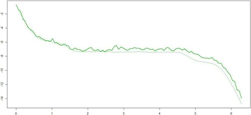A first way of assessing the quality of prediction is to compare predicted functional responses ($\hat{f}(\theta ,y,x)$ for any X in the testing sample) versus the true of conditional density operator (i.e., $f(\theta ,y,x)$) as in Figure 2.

Figure 2. Predicted functional responses (solid lines); observed functional responses (dashed lines).

For the next simulation algorithm, we used:

• Simulate a sample of size n.

• Calculate the smoothing parameters $h_K$ and $h_H$ that are varied over interval [0,1] and which minimizes (7(7) $\begin{array}{rl}& \frac{1}{n}\sum _{i=1}^n{W}_1\left(X_i\right)\int {\hat{f}}_{(h_K,h_H)}^{-i^2}(X_i,y)W_2\left(y\right)\mathrm{d}y\\ & -\frac{2}{n}\sum _{i=1}^n{\hat{f}}_{(h_K,h_H)}^{-i}(X_i,Y_i)W_1\left(X_i\right)W_2\left(Y_i\right),\end{array}$(7) ).

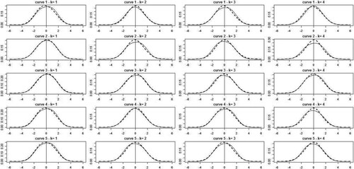
• Compute for k = 1, 2, 3, 4 the quantities $\left(n{h}_H{\varphi }_{{\theta }_k,x}{)}^{1/2}\right(\hat{f}({\theta }_k,y,x)-f({\theta }_k,y,x))$where $\hat{f}({\theta }_k,y,x)$ is the functional kernel estimator from the sample $(X_i,Y_i{)}_{i=1,\dots ,200,}$ and $k=1,2,3,4.$

• Compute a standard density estimator by local linear method.

• Compute the estimated $\hat{f}({\theta }_k,y,x)$ with the corresponding estimated $f({\theta }_k,y,x))$.

The obtained results are shown in Figure 3. It can be seen that both densities are very well approximated and have good behaviours with respect to the standard normal distribution.

Figure 3. Representation of the estimated density for k = 1, 2, 3, 4.

An application of results of Theorem 3.6 is to build the functional pseudo-confidence areas. To this aim, let us set for any component k, $(k=1,2,\dots ,K)$ and ${\eta }_k=\eta /K$ with $\eta \in [0,1]$, confidence intervals $E_k^{{\eta }_k}$ such that $P\left(\bigcap _{k=1}^K{r}_k\right(U)\in {\hat{E}}_K^{{\eta }_k})\ge 1-\eta$where $U=〈X,{\theta }_k〉$ with ${\theta }_1,\dots ,{\theta }_K$ being a data-driven orthonormal basis, the K eigenfunctions associated to the K largest eigenvalues of Γ.

The results from the asymptotic normality of the conditional density are expressed in Corollary 3.10 and we can approximate $(1-\eta )$ confidence interval of $f(\theta ,y,x)$ by $\hat{f}(\theta ,y,x)\pm t_{\eta /2}\times {\left(\frac{\widehat{V_{HK}}(\theta ,x,y)}{n{h}_H{\hat{\varphi }}_{\theta ,x}\left(h_K\right)}\right)}^{1/2},$where $t_{\eta /2}$ denotes the $\eta /2$ quantile of the standard normal $N(0,1)$.

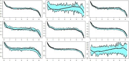
Figure 4 represents a functional pseudo-confidence zone for 9 different fixed curves with $\eta =0.05$ and K = 4. We see that $r(〈x,{\theta }_k〉)$ and its K-dimensional projection onto ${\hat{\theta }}_1,\dots ,{\hat{\theta }}_K$ are very close. This conclusion shows the good performance of our asymptotic normality. Indeed, when one replaces the data-driven basis with the eigenfunctions of Γ, one gets very similar functional pseudo-confidence areas.

Figure 4. Functional pseudo-confidence areas.

5. Conclusion

In this paper, we are mainly interested in the nonparametric estimation of the conditional density function by the local linear method for a variable explanatory functionally conditioned to an actual response variable via a functional single-index model. We show that the estimator provides good predictions under this model. One of the main contributions of this work is the choice of the semi-metric. Indeed, it is well known that, in nonparametric functional statistics, the semi-metric of the projection type is very important for increasing the concentration property. The functional index model is a special case of this family of semi-metrics because it is based on the projection on a functional direction which is important for the implementation of our method in practice. Therefore, we can draw zones of functional pseudo-confidence, which is a very interesting tool for assessing the quality of the prediction.

Acknowledgments

The authors are very grateful to the Editor and the anonymous reviewers for their comments which improved the quality of this paper. The authors wish to thank two anonymous referees for their helpful comments and suggestions, which greatly improved the quality of this paper.

Disclosure statement

No potential conflict of interest was reported by the author(s).

Appendix

Proof

Proof of Theorem 3.1

We know the theorem is a consequence of separately computing two quantities (bias and variance) of $\hat{f}(\theta ,y,x)$, and we have $\begin{array}{rl}& \mathbb{E}{\left[\hat{f}\right(\theta ,y,x)-f(\theta ,y,x\left)\right]}^2\\ & ={[\mathbb{E}\left(\hat{f}\right(\theta ,y,x\left)\right)-f(\theta ,y,x\left)\right]}^2+\mathrm{V}\mathrm{a}\mathrm{r}\left[\hat{f}\right(\theta ,y,x\left)\right].\end{array}$By classical calculations, we obtain $\begin{array}{rl}& \hat{f}(\theta ,y,x)-f(\theta ,y,x)\\ & =\left({\hat{f}}_N\right(\theta ,y,x)-f(\theta ,y,x\left)\right)\\ & -\left({\hat{f}}_N\right(\theta ,y,x)-\mathbb{E}[{\hat{f}}_N(\theta ,y,x)\left]\right)\left({\hat{f}}_D\right(\theta ,x)-1)\\ & -\mathbb{E}\left[{\hat{f}}_N\right(\theta ,y,x\left)\right]\left({\hat{f}}_D\right(\theta ,x)-1)\\ & +{\left({\hat{f}}_D\right(\theta ,x)-1)}^2\hat{f}(\theta ,y,x),\end{array}$which implies that $\begin{array}{rl}& \mathbb{E}\left[\hat{f}\right(\theta ,y,x\left)\right]-f(\theta ,y,x)\\ & =\left(\mathbb{E}\right[{\hat{f}}_N(\theta ,y,x)]-f(\theta ,y,x\left)\right)\\ & -\mathrm{C}\mathrm{o}\mathrm{v}\left({\hat{f}}_N\right(\theta ,y,x),{\hat{f}}_D(\theta ,x\left)\right)\\ & +\mathbb{E}\left[{\left({\hat{f}}_D\right(\theta ,x)-\mathbb{E}[{\hat{f}}_D(\theta ,x)\left]\right)}^2\hat{f}\right(\theta ,y,x\left)\right].\end{array}$Under the assumption (H5), we can bound $\hat{f}(\theta ,y,x)$ by a constant C>0 where $\hat{f}(\theta ,y,x)\le C/h_H$. Hence $\begin{array}{rl}& \mathbb{E}\left[\hat{f}\right(\theta ,y,x\left)\right]-f(\theta ,y,x)\\ & =\left(\mathbb{E}\right[{\hat{f}}_N(\theta ,y,x)]-f(\theta ,y,x\left)\right)\\ & -\mathrm{C}\mathrm{o}\mathrm{v}\left({\hat{f}}_N\right(\theta ,y,x),{\hat{f}}_D(\theta ,x\left)\right)\\ & +\mathrm{V}\mathrm{a}\mathrm{r}\left[{\hat{f}}_D\right(\theta ,x\left)\right]O\left(h_H^{-1}\right).\end{array}$Now, by similar techniques as those of Sarda and Vieu (2000) and by Bosq and Lecoutre (1987), the variance term is $\begin{array}{rl}& \mathrm{V}\mathrm{a}\mathrm{r}\left[\hat{f}\right(\theta ,y,x\left)\right]\\ & =\mathrm{V}\mathrm{a}\mathrm{r}\left[{\hat{f}}_N\right(\theta ,y,x\left)\right]\\ & -2\mathbb{E}\left[{\hat{f}}_N\right(\theta ,y,x\left)\right]\mathrm{C}\mathrm{o}\mathrm{v}\left({\hat{f}}_N\right(\theta ,y,x),{\hat{f}}_D(\theta ,x\left)\right)\\ & +{\left(\mathbb{E}\right[{\hat{f}}_N(\theta ,y,x)\left]\right)}^2\mathrm{V}\mathrm{a}\mathrm{r}\left({\hat{f}}_D\right(\theta ,x\left)\right)\\ & \times o\left(\frac{1}{n{h}_H{\varphi }_{\theta ,x}\left(h_K\right)}\right).\text{■}\end{array}$

Proof

Proof of Lemma 3.2

We have $\begin{array}{rl}& \mathbb{E}\left[{\hat{f}}_N\right(\theta ,y,x\left)\right]\\ & =\mathbb{E}[\phantom{\sum _{1\le i\ne j\le n}}\frac{1}{n(n-1)h_H\mathbb{E}\left[W_{12}\right(\theta ,x\left)\right]}\\ & \times \sum _{1\le i\ne j\le n}{W}_{ij}(\theta ,x)H\left(h_H^{-1}\right(y-Y_j\left)\right)]\\ & =\frac{1}{h_H\mathbb{E}\left[W_{\theta ,12}\right]}\mathbb{E}\left[W_{\theta ,12}\mathbb{E}\right[H_2|X_2\left]\right].\end{array}$By using a Taylor's expansion and under assumption (H5), we have $\begin{array}{rl}\mathbb{E}\left[H_2|X_2\right]& =f(\theta ,y,X_2)\\ & +\frac{h_H^2}{2}(\int t^{2}H(t\left)\mathrm{d}t\right)\frac{{\mathrm{\partial }}^{2}f(\theta ,y,X_2)}{\mathrm{\partial }{y}^2}+o\left(h_H^2\right).\end{array}$Now, we can rewrite the above equation as $\begin{array}{rl}\mathbb{E}\left[H_2|X_2\right]& ={\psi }_0(X_2,y)\\ & +\frac{h_H^2}{2}(\int t^{2}H(t\left)\mathrm{d}t\right){\psi }_2(X_2,y)+o\left(h_H^2\right).\end{array}$Thus, we obtain $\begin{array}{rl}& \mathbb{E}\left[{\hat{f}}_N\right(\theta ,y,x\left)\right]\\ & =\frac{1}{E\left[W_{\theta ,12}\right]}(\phantom{(\int t^{2}H(t\left)\mathrm{d}t\right)}\mathbb{E}\left[W_{\theta ,12}{\psi }_2\right(X_2,y\left)\right]\\ & +(\int t^{2}H(t\left)\mathrm{d}t\right)\mathbb{E}\left[W_{\theta ,12}{\psi }_2\right(X_2,y\left)\right]+o\left(h_H^2\right)).\end{array}$According to Ferraty et al. (2007), for $l\in \{0,2\}$, we show that $\begin{array}{rl}& \mathbb{E}\left[W_{\theta ,12}{\psi }_l\right(X_2,y\left)\right]\\ & ={\psi }_l(x,y)\mathbb{E}\left[W_{\theta ,12}\right]+\mathbb{E}\left[W_{\theta ,12}\right({\psi }_l(X_2,y)-{\psi }_l(x,y)\left)\right]\\ & ={\psi }_l(x,y)\mathbb{E}\left[W_{\theta ,12}\right]\\ & +\mathbb{E}\left[W_{\theta ,12}\mathbb{E}\right[{\psi }_l(X_2,y)-{\psi }_l(x,y)|d_{\theta }(X_2,x)\left]\right]\\ & ={\psi }_l(x,y)\mathbb{E}\left[W_{\theta ,12}\right]+\mathbb{E}\left[W_{\theta ,12}{\mathrm{\Phi }}_l\right(d_{\theta }(X_2,x)\left)\right].\end{array}$Since ${\mathrm{\Phi }}_l\left(0\right)=0$, we obtain $\begin{array}{rl}& \mathbb{E}\left[W_{\theta ,12}{\mathrm{\Phi }}_l\right(d_{\theta }(X_2,x)\left)\right]\\ & ={\mathrm{\Phi }}_l^{\mathrm{\prime }}\left(0\right)\mathbb{E}\left[d_{\theta }\right(X_2,x\left)W_{\theta ,12}\right]+o\left(\mathbb{E}\left[d_{\theta }\right(X_2,x\left)W_{\theta ,12}\right]\right).\end{array}$Then we get $\begin{array}{rl}\mathbb{E}\left[{\hat{f}}_N\right(\theta ,y,x\left)\right]& =f(\theta ,y,x)+\frac{h_H^2}{2}\frac{{\mathrm{\partial }}^{2}f(\theta ,y,x)}{\mathrm{\partial }{y}^2}\int t^{2}H\left(t\right)\mathrm{d}t\\ & +o\left(h_H^2\frac{\mathbb{E}\left[d_{\theta }\right(X_2,x\left)W_{\theta ,12}\right]}{\mathbb{E}\left[W_{\theta ,12}\right]}\right)\\ & +{\mathrm{\Phi }}_0^{\mathrm{\prime }}\left(0\right)\frac{\mathbb{E}\left[d_{\theta }\right(X_2,x\left)W_{\theta ,12}\right]}{\mathbb{E}\left[W_{\theta ,12}\right]}\\ & +o\left(\frac{\mathbb{E}\left[d_{\theta }\right(X_2,x\left)W_{\theta ,12}\right]}{\mathbb{E}\left[W_{\theta ,12}\right]}\right).\end{array}$Therefore, it remains to determine the quantities $\mathbb{E}\left[d_{\theta }\right(X_2,x\left)W_{\theta ,12}\right]$ and $\mathbb{E}\left[W_{\theta ,12}\right]$. According to the definition of $W_{\theta ,12}$, the two quantities $\mathbb{E}\left[d_{\theta }\right(X_2,x\left)W_{\theta ,12}\right]$ and $\mathbb{E}\left[W_{\theta ,12}\right]$ are based on the evaluation asymptotic of $\mathbb{E}\left[K_1^a{\text{β}}_1^b\right]$. To do that, we treat firstly, the case b = 1. For this case, we use the assumptions (H3) and (H4) to get $\begin{array}{rl}{h}_K\mathbb{E}\left[K_1^a{\text{β}}_{\theta ,1}\right]& =o\left({\int }_{B(x,h_K)}{\text{β}}_{\theta }^2\right(u,x\left)\mathrm{d}P\right(u\left)\right)\\ & =o\left(h_K^2{\varphi }_{\theta ,x}\right(h_K\left)\right).\end{array}$So, we obtain that, (A1) $\mathbb{E}\left[K_1^a{\text{β}}_{\theta ,1}\right]=o\left(h_K{\varphi }_{\theta ,x}\right(h_K\left)\right).$(A1) Moreover, for all b>1, and after simplifications of the expressions, it is permitted to write that $\mathbb{E}\left[K_1^a{\text{β}}_{\theta ,1}^b\right]=\mathbb{E}\left[K_1^a{d}_{\theta }^b\right(x,X\left)\right]+o\left(h_K^b{\varphi }_{\theta ,x}\right(h_K\left)\right).$Concerning the first term, we write $\begin{array}{rl}& h_K^{-b}\mathbb{E}\left[K_1^a{d}_{\theta }^b\right]\\ & =\int v^b{K}^a\left(v\right)\mathrm{d}{P}^{h_K^{-1}{d}_{\theta }(x,X)}\left(v\right)\\ & ={\int }_{-1}^1\left[K^a\right(1)-{\int }_v^1\left(\right(s^b{K}^a\left(s\right){)}^{\mathrm{\prime }})\mathrm{d}u]\mathrm{d}{P}^{h_K^{-1}{d}_{\theta }(x,X)}\left(v\right)\\ & =\left(K\right(1\left){\varphi }_{\theta ,x}\right(h_K)-{\int }_{-1}^1(s^b{K}^a\left(s\right){)}^{\left(1\right)}{\varphi }_{\theta ,x}(s{h}_K,h_K)\mathrm{d}s)\\ & ={\varphi }_{\theta ,x}\left(h_K\right)\left(K\right(1)-{\int }_{-1}^1(s^b{K}^a\left(s\right){)}^{\mathrm{\prime }}\frac{{\varphi }_{\theta ,x}(s{h}_K,h_K)}{{\varphi }_{\theta ,x}\left(h_K\right)}\mathrm{d}s).\end{array}$Finally, under assumptions (H1), we get (A2) $\begin{array}{rl}\mathbb{E}\left[K_1^a{\text{β}}_{\theta 1}^b\right]& =h_K^b{\varphi }_{\theta ,x}\left(h_K\right)\left(K\right(1)-{\int }_{-1}^1(s^b{K}^a\left(u\right){)}^{\mathrm{\prime }}{\chi }_{\theta ,x}\left(s\right)\mathrm{d}s)\\ & +o\left(h_K^b{\varphi }_{\theta ,x}\right(h_K\left)\right).\end{array}$(A2) So, $\begin{array}{rl}& \frac{\mathbb{E}\left[d_{\theta }\right(X_2,x\left)W_{\theta ,12}\right]}{\mathbb{E}\left[W_{\theta ,12}\right]}\\ & =h_K\left(\frac{K\left(1\right)-{\int }_{-1}^1\left(sK\right(s\left){)}^{\mathrm{\prime }}{\chi }_{\theta ,x}\right(s)\mathrm{d}s}{K\left(1\right)-{\int }_{-1}^1\left(K^{\mathrm{\prime }}\right(u\left){\chi }_{\theta ,x}\right(s)\mathrm{d}s}\right)+o\left(h_K\right).\end{array}$Hence, $\begin{array}{rl}& \mathbb{E}\left[{\hat{f}}_N\right(\theta ,y,x\left)\right]\\ & =f(\theta ,y,x)+\frac{h_H^2}{2}\frac{{\mathrm{\partial }}^{2}f(\theta ,y,x)}{\mathrm{\partial }{y}^2}\int t^{2}H\left(t\right)\mathrm{d}t+o\left(h_H^2\right)\\ & +h_K{\mathrm{\Phi }}_0^{\mathrm{\prime }}\left(0\right)\frac{\left(K\right(1)-{\int }_{-1}^1(sK\left(s\right){)}^{\mathrm{\prime }}{\chi }_{\theta ,x}\left(s\right)\mathrm{d}s)}{\left(K\right(1)-{\int }_{-1}^1{K}^{\mathrm{\prime }}(s\left){\chi }_{\theta ,x}\right(s\left)\mathrm{d}s\right)}\\ & +o\left(h_K\right).\text{■}\end{array}$

Proof

Proof of Lemma 3.3.

We know (A3) $\begin{array}{rl}& \mathrm{V}\mathrm{a}\mathrm{r}\left({\hat{f}}_N\right(\theta ,y,x\left)\right)\\ & =\frac{1}{{\left(n\right(n-1\left)h_H\right(\mathbb{E}\left[W_{\theta ,12}\right]\left)\right)}^2}\mathrm{V}\mathrm{a}\mathrm{r}\left(\sum _{1\le i\ne j\le n}{W}_{\theta ,ij}{H}_j\right)\\ & =\frac{1}{{\left(n\right(n-1\left)h_H\right(\mathbb{E}\left[W_{\theta ,12}\right]\left)\right)}^2}\\ & \times [n(n-1)\mathbb{E}\left[W_{\theta ,12}^2\right(H_2^2\left)\right]\\ & +n(n-1)\mathbb{E}\left[W_{\theta ,12}{W}_{\theta ,21}{H}_2{H}_1\right]\\ & +n(n-1)(n-2)\mathbb{E}\left[W_{\theta ,12}{W}_{\theta ,13}{H}_2{H}_3\right]\\ & +n(n-1)(n-2)\mathbb{E}\left[W_{\theta ,12}{W}_{\theta ,23}{H}_2{H}_3\right]\\ & +n(n-1)(n-2)\mathbb{E}\left[W_{\theta ,12}{W}_{\theta ,31}{H}_2{H}_1\right]\\ & +n(n-1)(n-2)\mathbb{E}\left[W_{\theta ,12}{W}_{\theta ,32}{H}_2^2\right]\\ & -n(n-1)(4n-6)\mathbb{E}[W_{\theta ,12}{H}_2{]}^2].\end{array}$(A3) By direct calculations, we get $\{\begin{array}{l}\mathbb{E}\left[W_{\theta ,12}^2{H}_2\right]=O\left(h_K^4{h}_H{\varphi }_{\theta ,x}^2\right(h_K\left)\right),\mathbb{E}\left[W_{\theta ,12}{W}_{\theta ,21}{H}_2{H}_1\right]\\ =O\left(h_K^4{h}_H^2{\varphi }_{\theta ,x}^2\right(h_K\left)\right),\\ \mathbb{E}\left[W_{\theta ,12}{W}_{\theta ,13}{H}_2{H}_3\right]=\mathbb{E}\left[W_{\theta ,12}{W}_{\theta ,31}{H}_2{H}_1\right]\\ =\mathbb{E}\left[W_{\theta ,12}{W}_{\theta ,23}{H}_2{H}_3\right]=O\left(h_K^4{h}_H^2{\varphi }_{\theta ,x}^3\right(h_K\left)\right),\\ \mathbb{E}\left[W_{\theta ,12}{W}_{\theta ,32}{H}_2^2\right]={\mathbb{E}}^2\left[{\text{β}}_1^2{K}_1\right]\mathbb{E}\left[K_1^2{H}_1^2\right]\\ +o\left(h_K^4{h}_H{\varphi }_{\theta ,x}^3\right(h_K\left)\right).\end{array}$Clearly, the latter term in the above equation is the leading one, and can be evaluated in (A3(A3) $\begin{array}{rl}& \mathrm{V}\mathrm{a}\mathrm{r}\left({\hat{f}}_N\right(\theta ,y,x\left)\right)\\ & =\frac{1}{{\left(n\right(n-1\left)h_H\right(\mathbb{E}\left[W_{\theta ,12}\right]\left)\right)}^2}\mathrm{V}\mathrm{a}\mathrm{r}\left(\sum _{1\le i\ne j\le n}{W}_{\theta ,ij}{H}_j\right)\\ & =\frac{1}{{\left(n\right(n-1\left)h_H\right(\mathbb{E}\left[W_{\theta ,12}\right]\left)\right)}^2}\\ & \times [n(n-1)\mathbb{E}\left[W_{\theta ,12}^2\right(H_2^2\left)\right]\\ & +n(n-1)\mathbb{E}\left[W_{\theta ,12}{W}_{\theta ,21}{H}_2{H}_1\right]\\ & +n(n-1)(n-2)\mathbb{E}\left[W_{\theta ,12}{W}_{\theta ,13}{H}_2{H}_3\right]\\ & +n(n-1)(n-2)\mathbb{E}\left[W_{\theta ,12}{W}_{\theta ,23}{H}_2{H}_3\right]\\ & +n(n-1)(n-2)\mathbb{E}\left[W_{\theta ,12}{W}_{\theta ,31}{H}_2{H}_1\right]\\ & +n(n-1)(n-2)\mathbb{E}\left[W_{\theta ,12}{W}_{\theta ,32}{H}_2^2\right]\\ & -n(n-1)(4n-6)\mathbb{E}[W_{\theta ,12}{H}_2{]}^2].\end{array}$(A3) ) by using $\frac{(n-2)}{n(n-1)\left(h_H\mathbb{E}\right[W_{\theta ,12}]{)}^2}{\mathbb{E}}^2\left[{\text{β}}_{\theta ,1}^2{K}_1\right]\mathbb{E}\left[K_1^2{H}_1^2\right].$By the same arguments used in the proof of Lemma 3.2, we obtain (A4) $\mathrm{V}\mathrm{a}\mathrm{r}\left({\hat{f}}_N\right(\theta ,y,x\left)\right)=\frac{\mathbb{E}\left[K_1^2{H}_1^2\right]}{n\left(h_H\mathbb{E}\right[K_1]{)}^2}+o\left(\frac{1}{n{h}_H{\varphi }_{\theta ,x}\left(h_K\right)}\right).$(A4) Observe that $\begin{array}{rl}\mathbb{E}\left[K_1^2{H}_1^2\right]& =\mathbb{E}\left[K_1^2\mathbb{E}\right((H_1^{\left(1\right)}{)}^2|〈\theta ,X_1〉)]\\ & =\mathbb{E}[K_1^2\int H^2(h_H^{-1}(y-z)\left)f\right(\theta ,z,X_1\left)\mathrm{d}z\right].\end{array}$Thus, by the change of variables $t=h_H^{-1}(y-z)$, we get $\mathbb{E}\left[K_1^2{H}_1^2\right]=h_H\mathbb{E}[K_1^2\int H^2(t\left)f\right(\theta ,y-h_{H}t,X_1\left)\mathrm{d}t\right].$By using Taylor's expansion of order 1 of $f(\theta ,\cdot ,y)$ we get $\begin{array}{rl}f(\theta ,y-h_{H}t,X_1)& =f(\theta ,y,X_1)+O\left(h_H\right)\\ & =f(\theta ,y,X_1)+o\left(1\right).\end{array}$Then $\begin{array}{rl}\mathbb{E}\left[K_1^2{H}_1^2\right]& =h_H(\int H^2(t\left)\mathrm{d}t\right)\mathbb{E}[K_1^{2}f(\theta ,y,X_1)]\\ & +o\left(h_H\mathbb{E}\right[K_1^2\left]\right).\end{array}$Also, by the same steps in the proof of Lemma 3.2, we obtain $\mathbb{E}[K_1^{2}f(\theta ,y,X_1)]=f(\theta ,y,x)\mathbb{E}\left[K_1^2\right]+o\left(\mathbb{E}\right[K_1^2\left]\right)$which give that (A5) $\mathbb{E}\left[K_1^2{H}_1^2\right]=h_{H}f(\theta ,y,x)\mathbb{E}\left[K_1^2\right]\int H^2\left(t\right)\mathrm{d}t+o\left(h_H\mathbb{E}\right[K_1^2\left]\right).$(A5) Finally, we obtain from (A2(A2) $\begin{array}{rl}\mathbb{E}\left[K_1^a{\text{β}}_{\theta 1}^b\right]& =h_K^b{\varphi }_{\theta ,x}\left(h_K\right)\left(K\right(1)-{\int }_{-1}^1(s^b{K}^a\left(u\right){)}^{\mathrm{\prime }}{\chi }_{\theta ,x}\left(s\right)\mathrm{d}s)\\ & +o\left(h_K^b{\varphi }_{\theta ,x}\right(h_K\left)\right).\end{array}$(A2) ), (A4(A4) $\mathrm{V}\mathrm{a}\mathrm{r}\left({\hat{f}}_N\right(\theta ,y,x\left)\right)=\frac{\mathbb{E}\left[K_1^2{H}_1^2\right]}{n\left(h_H\mathbb{E}\right[K_1]{)}^2}+o\left(\frac{1}{n{h}_H{\varphi }_{\theta ,x}\left(h_K\right)}\right).$(A4) ) and (A5(A5) $\mathbb{E}\left[K_1^2{H}_1^2\right]=h_{H}f(\theta ,y,x)\mathbb{E}\left[K_1^2\right]\int H^2\left(t\right)\mathrm{d}t+o\left(h_H\mathbb{E}\right[K_1^2\left]\right).$(A5) ), that $\begin{array}{rl}& \mathrm{V}\mathrm{a}\mathrm{r}\left({\hat{f}}_N\right(\theta ,y,x\left)\right)\\ & =\frac{f(\theta ,y,x)}{n{h}_H{\varphi }_{\theta ,x}\left(h_K\right)}(\int H^2(t\left)\mathrm{d}t\right)\\ & \times \left[\frac{\left(K^2\right(1)-{\int }_{-1}^1(K^2\left(s\right){)}^{\mathrm{\prime }}{\chi }_{\theta ,x}\left(s\right)\mathrm{d}s)}{{\left(K\right(1)-{\int }_{-1}^1(K\left(s\right){)}^{\mathrm{\prime }}{\chi }_{\theta ,x}\left(s\right)\mathrm{d}s)}^2}\right]\\ & +o\left(\frac{1}{n{h}_H{\varphi }_{\theta ,x}\left(h_K\right)}\right)\\ & =\frac{M_{2}f(\theta ,y,x)}{M_1^{2}n{h}_H{\varphi }_{\theta ,x}\left(h_K\right)}(\int H^2(t\left)\mathrm{d}t\right)\\ & +o\left(\frac{1}{n{h}_H{\varphi }_{\theta ,x}\left(h_K\right)}\right).\text{■}\end{array}$

Proof

Proof of Lemma 3.4

The proof of this Lemma is similar to the proof of Lemma 3.3. We can write $\begin{array}{rl}& \mathrm{C}\mathrm{o}\mathrm{v}\left({\hat{f}}_N\right(\theta ,y,x),{\hat{f}}_D(\theta ,x\left)\right)\\ & =\frac{1}{{\left(n\right(n-1\left)h_H\mathbb{E}\right[W_{\theta ,12}\left]\right)}^2}\\ & \times \mathrm{C}\mathrm{o}\mathrm{v}(\sum _{1\le i\ne j\le n}{W}_{\theta ,ij}{H}_j,\sum _{1\le i^{\mathrm{\prime }}\ne j^{\mathrm{\prime }}\le n}{W}_{\theta ,i^{\mathrm{\prime }}{j}^{\mathrm{\prime }}})\\ & =\frac{1}{{\left(n\right(n-1\left)h_H\mathbb{E}\right[W_{\theta ,12}\left]\right)}^2}[n(n-1)\mathbb{E}\left[W_{\theta 12}^2{H}_1\right]\\ & +n(n-1)\mathbb{E}\left[W_{\theta ,12}{W}_{\theta ,21}{H}_2\right]\\ & +n(n-1)(n-2)\mathbb{E}\left[W_{\theta ,12}{W}_{\theta ,13}{H}_2\right]\\ & +n(n-1)(n-2)\mathbb{E}\left[W_{\theta ,12}{W}_{\theta ,23}{H}_2\right]\\ & +n(n-1)(n-2)\mathbb{E}\left[W_{\theta ,12}{W}_{\theta ,31}{H}_2\right]\\ & +n(n-1)(n-2)\mathbb{E}\left[W_{\theta ,12}{W}_{\theta ,32}{H}_2\right]\\ & -n(n-1)(4n-6)\left(\mathbb{E}\right[W_{\theta ,12}{H}_2\left]\mathbb{E}\right[W_{\theta ,12}]].\end{array}$By direct calculations, we get $\{\begin{array}{l}\mathbb{E}\left[W_{\theta ,12}^2{H}_2\right]=\mathbb{E}\left[W_{\theta ,12}{W}_{\theta ,21}{H}_2\right]=O\left(h_K^4{h}_H{\varphi }_{\theta ,x}^2\right(h_K\left)\right),\\ \mathbb{E}\left[W_{\theta ,12}{W}_{\theta ,13}{H}_2\right]=\mathbb{E}\left[W_{\theta ,12}{W}_{\theta ,31}{H}_2\right]\\ =O\left(h_K^4{h}_H{\varphi }_{\theta ,x}^3\right(h_K\left)\right),\\ \mathbb{E}\left[W_{\theta ,12}{W}_{\theta ,23}{H}_2\right]=\mathbb{E}\left[W_{\theta ,12}{W}_{\theta ,32}{H}_2\right]\\ =O\left(h_K^4{h}_H{\varphi }_{\theta ,x}^3\right(h_K\left)\right).\end{array}$Since $\mathbb{E}\left[W_{\theta ,12}\right]=O\left(h_K^2{\varphi }_{\theta ,x}^2\right(h_K\left)\right)$, we obtain $\mathrm{C}\mathrm{o}\mathrm{v}\left({\hat{f}}_N\right(\theta ,y,x),{\hat{f}}_D(\theta ,x\left)\right)=O\left(\frac{1}{n{\varphi }_{\theta ,x}\left(h_K\right)}\right).\text{■}$

Proof

Proof of Lemma 3.5

We have that $\mathrm{V}\mathrm{a}\mathrm{r}\left({\hat{f}}_D\right(\theta ,x\left)\right)=\frac{1}{\left(n\right(n-1\left)\mathbb{E}\right[W_{\theta ,12}]{)}^2}\mathrm{V}\mathrm{a}\mathrm{r}\left(\sum _{1\le i\ne j\le n}{W}_{\theta ,ij}\right).$Similarly to the proof of Lemma 3.3, we get $\mathrm{V}\mathrm{a}\mathrm{r}\left({\hat{f}}_D\right(\theta ,x\left)\right)=\frac{\mathbb{E}\left[K_1^2\right]}{n\left(\mathbb{E}\right[K_1]{)}^2}+o\left(\frac{1}{n{\varphi }_{\theta ,x}\left(h_K\right)}\right).$We have as $n⟶\mathrm{\infty }$, $\frac{1}{{\varphi }_{\theta ,x}\left(h_K\right)}\mathbb{E}\left[K_1^j\right]⟶M_j,j=1,2$ (see Ferraty et al., 2007). Then, we can write finally $\begin{array}{rl}\mathrm{V}\mathrm{a}\mathrm{r}\left({\hat{f}}_D\right(\theta ,x\left)\right)& =\frac{M_2{\varphi }_{\theta ,x}\left(h_K\right)}{n{\left(M_1{\varphi }_{\theta ,x}\right(h_K\left)\right)}^2}+o\left(\frac{1}{n{\varphi }_{\theta ,x}\left(h_K\right)}\right)\\ & =O\left(\frac{1}{n{\varphi }_{\theta ,x}\left(h_K\right)}\right).\text{■}\end{array}$

Proof

Proof of Lemma 3.8

We have $\begin{array}{rl}& \sqrt{n{h}_H{\varphi }_{\theta ,x}\left(h_K\right)}{Q}_n(\theta ,x,y)\\ & =\frac{\sqrt{n{h}_H{\varphi }_{\theta ,x}\left(h_K\right)}}{n\mathbb{E}\left({\mathrm{\Omega }}_1{K}_1\right)}\left(\sum _{j=1}^n{\mathrm{\Omega }}_j{K}_j\right(H_j-f(\theta ,y,x))\\ & -\mathbb{E}\left(\sum _{j=1}^n{\mathrm{\Omega }}_j{K}_j\right(H_j-f(\theta ,y,x)\left)\right).\end{array}$Then, combined with (4(4) $\begin{array}{rl}& Q_n(\theta ,x,y)\\ & ={\hat{f}}_N(\theta ,y,x)-f(\theta ,y,x){\hat{f}}_D(\theta ,x)\\ & -\mathbb{E}\left({\hat{f}}_N\right(\theta ,y,x)-f(\theta ,y,x\left){\hat{f}}_D\right(\theta ,x)\\ & ={\hat{f}}_N(\theta ,y,x)-f(\theta ,y,x){\hat{f}}_D(\theta ,x)-{\mathbb{B}}_n(\theta ,x,y),\end{array}$(4) ) implies that $\begin{array}{rl}& \sqrt{n{h}_H{\varphi }_{\theta ,x}\left(h_K\right)}{Q}_n(\theta ,x,y)\\ & =\frac{1}{n\mathbb{E}\left({\text{β}}_1^2{K}_1\right)}\sum _{i=1}^n{\text{β}}_i^2{K}_i\frac{\sqrt{n{h}_H{\varphi }_{\theta ,x}\left(h_K\right)}\mathbb{E}\left({\text{β}}_1^2{K}_1\right)}{\mathbb{E}\left({\mathrm{\Omega }}_1{K}_1\right)}\\ & \times \sum _{j=1}^n{K}_j(H_j-f(\theta ,y,x\left)\right)\\ & -\frac{1}{n\mathbb{E}\left({\text{β}}_1{K}_1\right)}\sum _{i=1}^n{\text{β}}_i{K}_i\frac{\sqrt{n{h}_H{\varphi }_{\theta ,x}\left(h_K\right)}\mathbb{E}\left({\text{β}}_1{K}_1\right)}{\mathbb{E}\left({\mathrm{\Omega }}_1{K}_1\right)}\\ & \times \sum _{j=1}^n{\text{β}}_j{K}_j(H_j-f(\theta ,y,x\left)\right)\\ & -\mathbb{E}(\phantom{\sum _{j=1}^n}\frac{1}{n\mathbb{E}\left({\text{β}}_1^2{K}_1\right)}\sum _{i=1}^n{\text{β}}_i^2{K}_i\frac{\sqrt{n{h}_H{\varphi }_{\theta ,x}\left(h_K\right)}\mathbb{E}\left({\text{β}}_1^2{K}_1\right)}{\mathbb{E}\left({\mathrm{\Omega }}_1{K}_1\right)}\\ & \times \sum _{j=1}^n{K}_j(H_j-f(\theta ,y,x\left)\right))\\ & +\mathbb{E}(\phantom{\sum _{j=1}^n}\frac{1}{n\mathbb{E}\left({\text{β}}_1{K}_1\right)}\sum _{i=1}^n{\text{β}}_i{K}_i\frac{\sqrt{n{h}_H{\varphi }_{\theta ,x}\left(h_K\right)}\mathbb{E}\left({\text{β}}_1{K}_1\right)}{\mathbb{E}\left({\mathrm{\Omega }}_1{K}_1\right)}\\ & \times \sum _{j=1}^n{\text{β}}_j{K}_j(H_j-f(\theta ,y,x\left)\right)).\end{array}$Denote $\begin{array}{rl}{S}_1& =\frac{1}{n\mathbb{E}\left({\text{β}}_1^2{K}_1\right)}\sum _{i=1}^n{\text{β}}_i^2{K}_i,\\ S_2& =\frac{\sqrt{n{h}_H{\varphi }_{\theta ,x}\left(h_K\right)}\mathbb{E}\left({\text{β}}_1^2{K}_1\right)}{\mathbb{E}\left({\mathrm{\Omega }}_1{K}_1\right)}\sum _{j=1}^n{K}_j(H_j-f(\theta ,y,x\left)\right),\\ S_3& =\frac{1}{n\mathbb{E}\left({\text{β}}_1{K}_1\right)}\sum _{i=1}^n{\text{β}}_i{K}_i\mathrm{a}\mathrm{n}\mathrm{d}\\ S_4& =\frac{\sqrt{n{h}_H{\varphi }_{\theta ,x}\left(h_K\right)}\mathbb{E}\left({\text{β}}_1{K}_1\right)}{\mathbb{E}\left({\mathrm{\Omega }}_1{K}_1\right)}\sum _{j=1}^n{\text{β}}_j{K}_j(H_j-f(\theta ,y,x\left)\right).\end{array}$It remains to show that, $\begin{array}{rl}& \sqrt{n{h}_H{\varphi }_{\theta ,x}\left(h_K\right)}{Q}_n(\theta ,x,y)\\ & =S_1{S}_2-S_3{S}_4-\mathbb{E}(S_1{S}_2-S_3{S}_4)\\ & =(S_1{S}_2-\mathbb{E}(S_1{S}_2\left)\right)-(S_3{S}_4-\mathbb{E}(S_3{S}_4\left)\right).\end{array}$Hence by Slutsky's theorem, to show (A3(A3) $\begin{array}{rl}& \mathrm{V}\mathrm{a}\mathrm{r}\left({\hat{f}}_N\right(\theta ,y,x\left)\right)\\ & =\frac{1}{{\left(n\right(n-1\left)h_H\right(\mathbb{E}\left[W_{\theta ,12}\right]\left)\right)}^2}\mathrm{V}\mathrm{a}\mathrm{r}\left(\sum _{1\le i\ne j\le n}{W}_{\theta ,ij}{H}_j\right)\\ & =\frac{1}{{\left(n\right(n-1\left)h_H\right(\mathbb{E}\left[W_{\theta ,12}\right]\left)\right)}^2}\\ & \times [n(n-1)\mathbb{E}\left[W_{\theta ,12}^2\right(H_2^2\left)\right]\\ & +n(n-1)\mathbb{E}\left[W_{\theta ,12}{W}_{\theta ,21}{H}_2{H}_1\right]\\ & +n(n-1)(n-2)\mathbb{E}\left[W_{\theta ,12}{W}_{\theta ,13}{H}_2{H}_3\right]\\ & +n(n-1)(n-2)\mathbb{E}\left[W_{\theta ,12}{W}_{\theta ,23}{H}_2{H}_3\right]\\ & +n(n-1)(n-2)\mathbb{E}\left[W_{\theta ,12}{W}_{\theta ,31}{H}_2{H}_1\right]\\ & +n(n-1)(n-2)\mathbb{E}\left[W_{\theta ,12}{W}_{\theta ,32}{H}_2^2\right]\\ & -n(n-1)(4n-6)\mathbb{E}[W_{\theta ,12}{H}_2{]}^2].\end{array}$(A3) ), it suffices to prove the following two claims: (A6) $\begin{array}{rl}& S_1{S}_2-\mathbb{E}\left(S_1{S}_2\right)\stackrel{D}{\to }\mathcal{N}(0,V_{HK}(\theta ,x,y\left)\right),\end{array}$(A6) (A7) $\begin{array}{rl}& S_3{S}_4-\mathbb{E}\left(S_3{S}_4\right)\stackrel{P}{\to }0,\end{array}$(A7) Proof of (A6(A6) $\begin{array}{rl}& S_1{S}_2-\mathbb{E}\left(S_1{S}_2\right)\stackrel{D}{\to }\mathcal{N}(0,V_{HK}(\theta ,x,y\left)\right),\end{array}$(A6) ) We can write that $\begin{array}{rl}& S_1{S}_2-\mathbb{E}\left(S_1{S}_2\right)\\ & =S_2-\mathbb{E}\left(S_2\right)+(S_1-1)S_2-\mathbb{E}\left(\right(S_1-1\left)S_2\right).\end{array}$By Slutsky's theorem, we get the following intermediate results: (A8) $(S_1-1)S_2-\mathbb{E}\left(\right(S_1-1\left)S_2\right)\stackrel{P}{\to }0$(A8) and (A9) $S_2-\mathbb{E}\left(S_2\right)\stackrel{D}{\to }\mathcal{N}(0,V_{HK}(\theta ,x,y\left)\right).$(A9) Concerning the proof of (A8(A8) $(S_1-1)S_2-\mathbb{E}\left(\right(S_1-1\left)S_2\right)\stackrel{P}{\to }0$(A8) ), by applying the Bienaymé–Tchebychv's inequality, we obtain for all $ϵ>0$ $\begin{array}{rl}& \mathbb{P}\left(|\right(S_1-1)S_2-\mathbb{E}((S_1-1)S_2)|>ϵ)\\ & \le \frac{\mathbb{E}\left(|\right(S_1-1)S_2-\mathbb{E}(S_1-1\left)S_2\right)|)}{ϵ}.\end{array}$Then, the Cauchy–Schwarz inequality implies that $\begin{array}{rl}& \mathbb{E}\left(|\right(S_1-1)S_2-\mathbb{E}((S_1-1)S_2\left)|\right)\\ & \le 2\mathbb{E}\left(|\right(S_1-1\left)S_2\right)|)\le 2\sqrt{\mathbb{E}\left(\right(S_1-1{)}^2)}\sqrt{\mathbb{E}\left(\right(S_2{)}^2)}.\end{array}$On one side, by using (A1(A1) $\mathbb{E}\left[K_1^a{\text{β}}_{\theta ,1}\right]=o\left(h_K{\varphi }_{\theta ,x}\right(h_K\left)\right).$(A1) ) and (A2(A2) $\begin{array}{rl}\mathbb{E}\left[K_1^a{\text{β}}_{\theta 1}^b\right]& =h_K^b{\varphi }_{\theta ,x}\left(h_K\right)\left(K\right(1)-{\int }_{-1}^1(s^b{K}^a\left(u\right){)}^{\mathrm{\prime }}{\chi }_{\theta ,x}\left(s\right)\mathrm{d}s)\\ & +o\left(h_K^b{\varphi }_{\theta ,x}\right(h_K\left)\right).\end{array}$(A2) ), we obtain $\begin{array}{rl}\mathbb{E}\left(\right(S_1-1{)}^2)& =\mathrm{V}\mathrm{a}\mathrm{r}\left(S_1\right)=\frac{1}{n^2{\mathbb{E}}^2\left({\text{β}}_1^2{K}_1\right)}n\mathrm{V}\mathrm{a}\mathrm{r}\left({\text{β}}_1^2{K}_1\right)\\ & \le \frac{1}{nO\left(h^4{\varphi }_{\theta ,x}^2\right(h_K\left)\right)}\mathbb{E}\left({\text{β}}_1^4{K}_1^2\right)\\ & =O\left(\frac{1}{n{h}_H{\varphi }_{\theta ,x}\left(h_K\right)}\right).\end{array}$And on the other side, we obtain $\begin{array}{rl}\mathbb{E}\left(\right(S_2{)}^2)& =\frac{n{h}_H{\varphi }_{\theta ,x}\left(h_K\right){\mathbb{E}}^2\left({\text{β}}_1^2{K}_1\right)}{{\mathbb{E}}^2\left({\mathrm{\Omega }}_1{K}_1\right)}\\ & \times \mathbb{E}{\left(\sum _{j=1}^n{K}_j\right(H_j-f(\theta ,y,x)\left)\right)}^2\\ & =\frac{n}{(n-1{)}^{2}O({\varphi }_{\theta ,x}\left(h_K\right))}\left(nO\right({\varphi }_{\theta ,x}\left(h_K\right))\\ & +n(n-1)o\left({\varphi }_{\theta ,x}^2\right(h_K\left)\right))\\ & =O\left(1\right)+o\left(n{\varphi }_{\theta ,x}^2\right(h_K\left)\right).\end{array}$Thus $\begin{array}{rl}& \mathbb{E}\left(|\right(S_1-1)S_2-\mathbb{E}((S_1-1)S_2\left)|\right)\\ & \le 2\sqrt{\mathbb{E}\left(\right(S_1-1{)}^2)}\sqrt{\mathbb{E}\left(\right(S_2{)}^2)}\\ & \le 2\sqrt{O\left(\frac{1}{n{h}_H{\varphi }_{\theta ,x}\left(h_K\right)}\right)\left(O\right(1)+o(n{h}_H{\varphi }_{\theta ,x}\left(h_K\right)\left)\right)}\\ & =o\left(1\right),\end{array}$which implies that $\left(S_1-1\right)S_2-\mathbb{E}\left(S_1-1\right)S_2)=o_p(1)$. Then, as $n\to \mathrm{\infty }$, we get $\begin{array}{rl}& \mathbb{P}\left(|\right(S_1-1)S_2-\mathbb{E}(S_1-1\left)S_2\right)|)>ϵ)\\ & \le \frac{\mathbb{E}\left(|\right(S_1-1)S_2-\mathbb{E}(S_1-1\left)S_2\right)|)}{ϵ}\to 0.\end{array}$Concerning the proof of (A9(A9) $S_2-\mathbb{E}\left(S_2\right)\stackrel{D}{\to }\mathcal{N}(0,V_{HK}(\theta ,x,y\left)\right).$(A9) ) $\begin{array}{rl}{P}_n& =S_2-\mathbb{E}\left(S_2\right)\\ & =\frac{\sqrt{n{h}_H{\varphi }_{\theta ,x}\left(h_K\right)}\mathbb{E}\left({\text{β}}_1^2{K}_1\right)}{\mathbb{E}\left({\mathrm{\Omega }}_1{K}_1\right)}\sum _{j=1}^n{K}_j(H_j-f(\theta ,y,x\left)\right)\\ & -\mathbb{E}\left(K_j\right(H_j-f(\theta ,y,x)\left)\right)\\ & =\frac{\sqrt{n{h}_H{\varphi }_{\theta ,x}\left(h_K\right)}\mathbb{E}\left({\text{β}}_1^2{K}_1\right)}{\mathbb{E}\left({\mathrm{\Omega }}_1{K}_1\right)}\sum _{j=1}^n{\mu }_{nj}(x,y),\end{array}$where ${\mu }_{nj}(x,y)=K_j(H_j-f(\theta ,y,x\left)\right)-\mathbb{E}\left(K_j\right(H_j-f(\theta ,y,x)\left)\right).$By the fact that ${\mu }_{nj}(x,y)$ are i.i.d., it follows that $\begin{array}{rl}\mathrm{v}\mathrm{a}\mathrm{r}\left(P_n\right(x,y\left)\right)& =\frac{n^2{\varphi }_{\theta ,x}\left(h_K\right){\mathbb{E}}^2\left({\text{β}}_1^2{K}_1\right)}{{\mathbb{E}}^2\left({\mathrm{\Omega }}_1{K}_1\right)}\mathrm{v}\mathrm{a}\mathrm{r}\left({\mu }_{n1}\right(x,y\left)\right)\\ & =\frac{n^2{\varphi }_{\theta ,x}\left(h_K\right){\mathbb{E}}^2\left({\text{β}}_1^2{K}_1\right)}{{\mathbb{E}}^2\left({\mathrm{\Omega }}_1{K}_1\right)}\mathbb{E}\left({\mu }_{n1}^2\right(x,y\left)\right).\end{array}$Thus (A10) $\begin{array}{rl}& \mathrm{v}\mathrm{a}\mathrm{r}\left(P_n\right(x,y\left)\right)\\ & =\frac{n^2{\varphi }_{\theta ,x}\left(h_K\right){\mathbb{E}}^2\left({\text{β}}_1^2{K}_1\right)}{{\mathbb{E}}^2\left({\mathrm{\Omega }}_1{K}_1\right)}\left(\mathbb{E}\right(K_1^2(H_1-f(\theta ,y,x\left){)}^2\right)\\ & -\left(\mathbb{E}\right(K_1(H_1-f(\theta ,y,x\left)\right){)}^2).\end{array}$(A10) Concerning the second term on the right-hand side of (A10(A10) $\begin{array}{rl}& \mathrm{v}\mathrm{a}\mathrm{r}\left(P_n\right(x,y\left)\right)\\ & =\frac{n^2{\varphi }_{\theta ,x}\left(h_K\right){\mathbb{E}}^2\left({\text{β}}_1^2{K}_1\right)}{{\mathbb{E}}^2\left({\mathrm{\Omega }}_1{K}_1\right)}\left(\mathbb{E}\right(K_1^2(H_1-f(\theta ,y,x\left){)}^2\right)\\ & -\left(\mathbb{E}\right(K_1(H_1-f(\theta ,y,x\left)\right){)}^2).\end{array}$(A10) ), we have $\begin{array}{rl}& \left(\mathbb{E}\right(K_1(H_1-f(\theta ,y,x\left)\right){)}^2\\ & =\left(\mathbb{E}\right(\mathbb{E}\left(K_1\right(H_1-f(\theta ,y,x)\left)|X_1\right){)}^2\\ & =\left(\mathbb{E}\right(K_1\mathbb{E}\left(\right(H_1|X_1)-f(\theta ,y,x\left)\right)){)}^2,\end{array}$where (A11) $\mathbb{E}\left(\right(H_1|X_1)-f(\theta ,y,x\left)\right)\to 0\mathrm{a}\mathrm{s}n\to \mathrm{\infty }.$(A11) Now let us return to the first term of the right hand of (A10(A10) $\begin{array}{rl}& \mathrm{v}\mathrm{a}\mathrm{r}\left(P_n\right(x,y\left)\right)\\ & =\frac{n^2{\varphi }_{\theta ,x}\left(h_K\right){\mathbb{E}}^2\left({\text{β}}_1^2{K}_1\right)}{{\mathbb{E}}^2\left({\mathrm{\Omega }}_1{K}_1\right)}\left(\mathbb{E}\right(K_1^2(H_1-f(\theta ,y,x\left){)}^2\right)\\ & -\left(\mathbb{E}\right(K_1(H_1-f(\theta ,y,x\left)\right){)}^2).\end{array}$(A10) ). We have $\begin{array}{rl}& \frac{n^2{\varphi }_{\theta ,x}\left(h_K\right){\mathbb{E}}^2\left({\text{β}}_1^2{K}_1\right)}{{\mathbb{E}}^2\left({\mathrm{\Omega }}_1{K}_1\right)}\left(\mathbb{E}\right(K_1^2(H_1-f(\theta ,y,x\left){)}^2\right)\\ & =\frac{n^2{\varphi }_{\theta ,x}\left(h_K\right){\mathbb{E}}^2\left({\text{β}}_1^2{K}_1\right)}{{\mathbb{E}}^2\left({\mathrm{\Omega }}_1{K}_1\right)}\left(\mathbb{E}\right(\mathbb{E}\left(\right(H_1-f(\theta ,y,x){)}^2|X_1\left)K_1^2\right)\\ & =\frac{n^2{\varphi }_{\theta ,x}\left(h_K\right){\mathbb{E}}^2\left({\text{β}}_1^2{K}_1\right)}{{\mathbb{E}}^2\left({\mathrm{\Omega }}_1{K}_1\right)}\mathbb{E}\left(var\right(H_1|X_1\left)K_1^2\right)\\ & +\frac{n^2{\varphi }_{\theta ,x}\left(h_K\right){\mathbb{E}}^2\left({\text{β}}_1^2{K}_1\right)}{{\mathbb{E}}^2\left({\mathrm{\Omega }}_1{K}_1\right)}\\ & \times \left(\mathbb{E}\right(\mathbb{E}\left(\right(H_1|X_1)-f(\theta ,y,x\left){)}^2\right)K_1^2)\end{array}$By using (A9(A9) $S_2-\mathbb{E}\left(S_2\right)\stackrel{D}{\to }\mathcal{N}(0,V_{HK}(\theta ,x,y\left)\right).$(A9) ), we have as $n\to \mathrm{\infty }$ $\frac{n^2{\varphi }_{\theta ,x}\left(h_K\right){\mathbb{E}}^2\left({\text{β}}_1^2{K}_1\right)}{{\mathbb{E}}^2\left({\mathrm{\Omega }}_1{K}_1\right)}\left(\mathbb{E}\right(\mathbb{E}\left(\right(H_1|X_1)-f(\theta ,y,x\left){)}^2\right)K_1^2)\to 0$Combining (5(5) $\begin{array}{rl}& \hat{f}(\theta ,y,x)-f(\theta ,y,x)-{\mathbb{B}}_n(\theta ,x,y)\\ & =\frac{Q_n(\theta ,x,y)-{\mathbb{B}}_n(\theta ,x,y)\left({\hat{f}}_D\right(\theta ,x)-\mathbb{E}({\hat{f}}_D(\theta ,x)\left)\right)}{{\hat{f}}_D(\theta ,x)}\end{array}$(5) ) and (6(6) $\sqrt{n{h}_H{\varphi }_{\theta ,x}\left(h_K\right)}{Q}_n(\theta ,x,y)\stackrel{D}{\to }\mathcal{N}(0,V_{HK}(\theta ,x,y\left)\right),$(6) ), we obtain as $n\to \mathrm{\infty }$ $\begin{array}{rl}\mathbb{E}\left(var\right(H_1|X_1\left)K_1^2\right)& \to \mathbb{E}\left(K_1^2\right)f(\theta ,y,x)(\int H^2(t\left)\mathrm{d}t\right)\\ & =M_{2}f(\theta ,y,x)(\int H^2(t\left)\mathrm{d}t\right){\varphi }_{\theta ,x}\left(h_K\right).\end{array}$Therefore, by using (5(5) $\begin{array}{rl}& \hat{f}(\theta ,y,x)-f(\theta ,y,x)-{\mathbb{B}}_n(\theta ,x,y)\\ & =\frac{Q_n(\theta ,x,y)-{\mathbb{B}}_n(\theta ,x,y)\left({\hat{f}}_D\right(\theta ,x)-\mathbb{E}({\hat{f}}_D(\theta ,x)\left)\right)}{{\hat{f}}_D(\theta ,x)}\end{array}$(5) ) and (6(6) $\sqrt{n{h}_H{\varphi }_{\theta ,x}\left(h_K\right)}{Q}_n(\theta ,x,y)\stackrel{D}{\to }\mathcal{N}(0,V_{HK}(\theta ,x,y\left)\right),$(6) ), Equation (A10(A10) $\begin{array}{rl}& \mathrm{v}\mathrm{a}\mathrm{r}\left(P_n\right(x,y\left)\right)\\ & =\frac{n^2{\varphi }_{\theta ,x}\left(h_K\right){\mathbb{E}}^2\left({\text{β}}_1^2{K}_1\right)}{{\mathbb{E}}^2\left({\mathrm{\Omega }}_1{K}_1\right)}\left(\mathbb{E}\right(K_1^2(H_1-f(\theta ,y,x\left){)}^2\right)\\ & -\left(\mathbb{E}\right(K_1(H_1-f(\theta ,y,x\left)\right){)}^2).\end{array}$(A10) ) becomes $\begin{array}{rl}& \mathrm{V}\mathrm{a}\mathrm{r}\left(P_n\right(x,y\left)\right)\\ & =\frac{n^2{\varphi }_{\theta ,x}\left(h_K\right)\left(N\right(1,2\left)h_K^2{\varphi }_{\theta ,x}\right(h_K){)}^2}{\left(\right(n-1\left)N\right(1,2\left)M_1{h}_K^2{\varphi }_{\theta ,x}\right(h_K){)}^2}{M}_{2}f(\theta ,y,x)\\ & \times (\int H^2(t\left)\mathrm{d}t\right){\varphi }_{\theta ,x}\left(h_K\right)\\ & =\frac{n^2{M}_2}{(n-1{)}^2{M}_1^2}f(\theta ,y,x)(\int H^2(t\left)\mathrm{d}t\right)\\ & \to \frac{M_2}{M_1^2}f(\theta ,y,x)(\int H^2(t\left)\mathrm{d}t\right)\\ & =V_{HK}(\theta ,x,y)\mathrm{a}\mathrm{s}n\to \mathrm{\infty }.\end{array}$Now, in order to end the proof of (A6(A6) $\begin{array}{rl}& S_1{S}_2-\mathbb{E}\left(S_1{S}_2\right)\stackrel{D}{\to }\mathcal{N}(0,V_{HK}(\theta ,x,y\left)\right),\end{array}$(A6) ), we focus on the central limit theorem. So, the proof of (13) is completed if Lindberg's condition is verified. In fact, Lindberg's condition holds since, for any $\eta >0$ $\begin{array}{rl}\sum _{j=1}^n\mathbb{E}\left({\mu }_{nj}^2{\text{𝟙}}_{(|{\mu }_{nj}|>\eta )}\right)& =n\mathbb{E}\left({\mu }_{n1}^2{\text{𝟙}}_{(|{\mu }_{n1}|>\eta )}\right)\\ & =\mathbb{E}\left(\right(\sqrt{n}{\mu }_{n1}{)}^2{\text{𝟙}}_{(|\sqrt{n}{\mu }_{n1}|>\sqrt{n}\eta )})\end{array}$as $\mathbb{E}\left(\right(\sqrt{n}{\mu }_{n1}{)}^2)=n\mathbb{E}({\mu }_{n1}^2)\to \frac{M_2}{M_1^2}f(\theta ,y,x)(\int H^2(t\left)\mathrm{d}t\right).$Proofs of (A7(A7) $\begin{array}{rl}& S_3{S}_4-\mathbb{E}\left(S_3{S}_4\right)\stackrel{P}{\to }0,\end{array}$(A7) ) To use the same arguments as those invoked to prove (A6(A6) $\begin{array}{rl}& S_1{S}_2-\mathbb{E}\left(S_1{S}_2\right)\stackrel{D}{\to }\mathcal{N}(0,V_{HK}(\theta ,x,y\left)\right),\end{array}$(A6) ), let us write $\begin{array}{rl}& S_3{S}_4-\mathbb{E}\left(S_3{S}_4\right)\\ & =S_4-\mathbb{E}\left(S_4\right)+(S_3-1)S_4-\mathbb{E}(S_3-1)S_4.\end{array}$By applying Bienaymé–Tchebychv's inequality, we obtain for all $ϵ>0$ $\mathbb{P}(|S_3{S}_4-\mathbb{E}(S_3{S}_4\left)|\right)>ϵ)\le \frac{\mathbb{E}(|S_3{S}_4-\mathbb{E}(S_3{S}_4\left)|\right)}{ϵ}.$And the Cauchy–Schwarz inequality implies that $\begin{array}{rl}& \mathbb{E}\left(|\right(S_3-1)S_4-\mathbb{E}((S_3-1)S_4\left)|\right)\\ & \le 2\mathbb{E}\left(|\right(S_3-1\left)S_4\right)|)\le 2\sqrt{\mathbb{E}\left(\right(S_3-1{)}^2)}\sqrt{\mathbb{E}\left(\right(S_4{)}^2)}.\end{array}$Taking into account the assumptions H(5(5) $\begin{array}{rl}& \hat{f}(\theta ,y,x)-f(\theta ,y,x)-{\mathbb{B}}_n(\theta ,x,y)\\ & =\frac{Q_n(\theta ,x,y)-{\mathbb{B}}_n(\theta ,x,y)\left({\hat{f}}_D\right(\theta ,x)-\mathbb{E}({\hat{f}}_D(\theta ,x)\left)\right)}{{\hat{f}}_D(\theta ,x)}\end{array}$(5) ) and H(6(6) $\sqrt{n{h}_H{\varphi }_{\theta ,x}\left(h_K\right)}{Q}_n(\theta ,x,y)\stackrel{D}{\to }\mathcal{N}(0,V_{HK}(\theta ,x,y\left)\right),$(6) ), we get $\begin{array}{rl}\mathbb{E}\left(\right(S_3-1{)}^2& =\mathrm{V}\mathrm{a}\mathrm{r}\left(S_3\right)=\frac{n}{n^2{\mathbb{E}}^2\left({\text{β}}_1{K}_1\right)}\mathrm{v}\mathrm{a}\mathrm{r}\left({\text{β}}_1{K}_1\right)\\ & \le \frac{1}{nO\left(h^4{\varphi }_{\theta ,x}^2\right(h_K\left)\right)}\mathbb{E}\left({\text{β}}_1^4{K}_1^2\right)\\ & =O\left(\frac{1}{n{h}_H{\varphi }_{\theta ,x}\left(h_K\right)}\right).\end{array}$On the other hand, $\begin{array}{rl}\mathbb{E}\left(\right(S_4{)}^2)& =\frac{n{h}_H{\varphi }_{\theta ,x}\left(h_K\right){\mathbb{E}}^2\left({\text{β}}_1{K}_1\right)}{{\mathbb{E}}^2\left({\mathrm{\Omega }}_1{K}_1\right)}\\ & \times \mathbb{E}{\left(\sum _{j=1}^n{\text{β}}_j{K}_j\right(H_j-f(\theta ,y,x)\left)\right)}^2\\ & =\frac{n{h}_H{\varphi }_{\theta ,x}\left(h_K\right)O\left(h_K^2{\varphi }_{\theta ,x}^2\right(h_K\left)\right)}{(n-1{)}^{2}O(h_K^4{\varphi }_{\theta ,x}^4\left(h_K\right))}\\ & \times \left(n\mathbb{E}\right({\text{β}}_1{K}_1(H_1-f(\theta ,y,x\left)\right)){)}^2\\ & +n(n-1){\mathbb{E}}^2\left({\text{β}}_1{K}_1\right(H_1-f(\theta ,y,x)\left)\right)\\ & =o\left(1\right)+o\left(n{h}_H{\varphi }_{\theta ,x}\right(h_K\left)\right).\end{array}$It remains to show $\begin{array}{rl}& \mathbb{E}\left(|\right(S_3-1)S_4-\mathbb{E}((S_3-1)S_4\left)|\right)\\ & \le 2\sqrt{\mathbb{E}\left(\right(S_3-1{)}^2)}\sqrt{\mathbb{E}\left(\right(S_4{)}^2)}=o\left(1\right)\end{array}$ which implies that $\mathbb{E}\left(|\right(S_3-1)S_4-\mathbb{E}((S_3-1)S_4\left)|\right)=o_p\left(1\right).$Therefore, $\begin{array}{rl}& \mathbb{P}(|S_3{S}_4-\mathbb{E}(S_3{S}_4\left)|\right)>ϵ)\\ & \le \frac{\mathbb{E}(|S_3{S}_4-\mathbb{E}(S_3{S}_4\left)|\right)}{ϵ}\to 0\mathrm{a}\mathrm{s}n\to \mathrm{\infty }.\end{array}$So, to prove (A6(A6) $\begin{array}{rl}& S_1{S}_2-\mathbb{E}\left(S_1{S}_2\right)\stackrel{D}{\to }\mathcal{N}(0,V_{HK}(\theta ,x,y\left)\right),\end{array}$(A6) ), it suffices to show $S_4-\mathbb{E}\left(S_4\right)=o\left(1\right)$, while $\begin{array}{rl}\mathbb{E}(S_4-\mathbb{E}(S_4){)}^2& =\mathrm{V}\mathrm{a}\mathrm{r}\left(S_4\right)\\ & =\frac{n^2{\varphi }_{\theta ,x}\left(h_K\right){\mathbb{E}}^2\left({\text{β}}_1{K}_1\right)}{{\mathbb{E}}^2\left({\mathrm{\Omega }}_1{K}_1\right)}\\ & \times \mathrm{V}\mathrm{a}\mathrm{r}\left({\text{β}}_1{K}_1\right(H_1-f(\theta ,y,x)\left)\right).\end{array}$We arrive finally at $\begin{array}{rl}& \mathrm{V}\mathrm{a}\mathrm{r}\left({\text{β}}_1{K}_1\right(H_1-f(\theta ,y,x)\left)\right)\\ & =f(\theta ,y,x)(\int H^2(t\left)\mathrm{d}t\right)\mathbb{E}\left({\text{β}}_1^2{K}_1^2\right).\end{array}$This last result together with (5(5) $\begin{array}{rl}& \hat{f}(\theta ,y,x)-f(\theta ,y,x)-{\mathbb{B}}_n(\theta ,x,y)\\ & =\frac{Q_n(\theta ,x,y)-{\mathbb{B}}_n(\theta ,x,y)\left({\hat{f}}_D\right(\theta ,x)-\mathbb{E}({\hat{f}}_D(\theta ,x)\left)\right)}{{\hat{f}}_D(\theta ,x)}\end{array}$(5) ) and (6(6) $\sqrt{n{h}_H{\varphi }_{\theta ,x}\left(h_K\right)}{Q}_n(\theta ,x,y)\stackrel{D}{\to }\mathcal{N}(0,V_{HK}(\theta ,x,y\left)\right),$(6) ) leads directly to $\begin{array}{rl}& \mathbb{E}(S_4-\mathbb{E}(S_4){)}^2\\ & =\frac{n^2{\varphi }_{\theta ,x}\left(h_K\right){\mathbb{E}}^2\left({\text{β}}_1{K}_1\right)}{{\mathbb{E}}^2\left({\mathrm{\Omega }}_1{K}_1\right)}f(\theta ,y,x)(\int H^2(t\left)\mathrm{d}t\right)\mathbb{E}\left({\text{β}}_1^2{K}_1^2\right)\\ & =f(\theta ,y,x)(\int H^2(t\left)\mathrm{d}t\right)o\left(1\right),\end{array}$which allows finishes the proof.

References

- Ait Saidi, A., Ferraty, F., Kassa, P., & Vieu, P. (2008). Cross-validated estimations in the single functional index model. Statistics, 42(6), 475–494. https://doi.org/10.1080/02331880801980377
- Attaoui, S. (2014). Strong uniform consistency rates and asymptotic normality of conditional density estimator in the single functional index modeling for time series data. AStA Advances in Statistical Analysis., 98(3), 257–286. https://doi.org/10.1007/s10182-014-0227-3
- Attaoui, S., Laksaci, A., & Ould Said, F. (2011). A note on the conditional density estimate in the single functional index model. Statistics & Probability Letters, 81(1), 45–53. https://doi.org/10.1016/j.spl.2010.09.017
- Attaoui, S., & Ling, N. (2016). Asymptotic results of a nonparametric conditional cumulative distribution estimator in the single functional index modeling for time series data with applications. Metrika, 79(3), 485–511. https://doi.org/10.1007/s00184-015-0564-6
- Baìllo, A., & Grané, A. (2009). Local linear regression for functional predictor and scalar response. Journal of Multivariate Analysis, 100(1), 102–111. https://doi.org/10.1016/j.jmva.2008.03.008
- Barrientos-Marin, J., Ferraty, F., & Vieu, P. (2010). Locally modelled regression and functional data. Journal of Nonparametric Statistics, 22(5), 617–632. https://doi.org/10.1080/10485250903089930
- Bosq, D., & Lecoutre, J. P. (1987). Théorie de l'estimation fonctionnelle. Ed. Economica.
- Demongeot, J., Laksaci, A., Madani, F., & Rachdi, M. (2013). Functional data: local linear estimation of the conditional density and its application. Statistics: A Journal of Theoretical and Applied Statistics., 76(2), 328–355. https://doi.org/10.1080/02331888.2011.568117
- Demongeot, J., Laksaci, A., Rachdi, M., & Rahmani, S. (2014). On the local linear modelization of the conditional distribution for functional data. Sankhya: The Indian Journal of Statistics., 76(2), 328–355. https://doi.org/10.1007/s13171-013-0050-z
- Ferraty, F., Laksaci, A., Tadj, A., & Vieu, P. (2010). Rate of uniform consistency for nonparametric estimates with functional variables. Journal of Statistical Planning and Inference, 140(2), 335–352. https://doi.org/10.1016/j.jspi.2009.07.019
- Ferraty, F, Laksaci, A, & Vieu, P. (2006). Estimating some characteristics of the conditional distribution in nonparametric functional model. Statistical Inference for Stochastic Processes , 9(1), 47–76. https://doi.org/10.1007/s.11203-004-3561-3
- Ferraty, F., Mas, A., Vieu, P., & Vieu, P. (2007). Advances in nonparametric regression for functional variables. Australian & New Zealand Journal of Statistics, 49(1), 1–20. https://doi.org/10.1111/j.1467-842X.2006.00454.x
- Ferraty, F., Peuch, A., & Vieu, P. (2003). Modéle à indice fonctionnel simple. Comptes Rendus Mathématique de l'Académie des Sciences Paris, 336(12), 1025–1028. https://doi.org/10.1016/S1631-073X(03)00239-5(in French)
- Ferraty, F., & Vieu, P. (2006). Nonparametric functional data analysis. Theory and Practice. Springer Series in Statistics.
- Laksaci, A. (2007). Convergence en moyenne quadratique de l'estimateur a noyau de la densité conditionnelle avec variable explicative fonctionnelle. Publications de l'Institut de statistique de l'Université de Paris, 51(3), 69–80.
- Laksaci, A., Rachdi, M., & Rahmani, S. (2013). Spatial modelization: local linear estimation of the conditional distribution for functional data. Spatial Statistics, 6(4), 1–23. https://doi.org/10.1016/j.spasta.2013.04.004
- Masry, E. (2005). Nonparametric regression estimation for dependent functional data: asymptotic normality. Stochastic Processes and their Applications, 115(1), 155–177. https://doi.org/10.1016/j.spa.2004.07.006
- Sarda, P., & Vieu, P. (2000). Kernel regression. Wiley Series in Probability and Statistics (pp. 43–70).
- Tabti, H., & Ait Saidi, A. (2018). Estimation and simulation of conditional hazard function in the quasi-associated framework when the observations are linked via a functional single-index structure. Communications in Statistics -- Theory and Methods, 47(4), 816–838. https://doi.org/10.1080/03610926.2016.1213294