
 ?Mathematical formulae have been encoded as MathML and are displayed in this HTML version using MathJax in order to improve their display. Uncheck the box to turn MathJax off. This feature requires Javascript. Click on a formula to zoom.
Abstract
In a repairable consecutive system, after the system operates for a certain time, some components may fail, some failed components may be repaired and the state of the system may change. The models developed in the existing literature usually assume that the state of the system varies over time depending on the values of n and k and the state of the system is known. Since the system reliability will vary over time, it is of great interest to analyse the time-dependent system reliability. In this paper, we develop a novel and simple method that utilizes the eigenvalues of the transition rate matrix of the system for the computation of time-dependent system reliability when the system state is known. In addition, the transition performance probabilities of the system from a known state to the possible states are also analysed. Computational results are presented to illustrate the applicability and accuracy of the proposed method.
1. Introduction
In many engineering applications, consecutive-k-out-of-n systems are encountered and the evaluation of the system reliability is of interest. For example, consecutive-k-out-of-n systems appear in telecommunications, microwave relay stations, oil pipeline systems, vacuum systems in accelerators, computer ring networks and spacecraft relay stations. These systems can be classified with respect to the logical or physical connections among components as either linear or circular and the functioning principle as either failed (F) or good (G). A consecutive-k-out-of-n: F system, or a system for short, consists of an ordered sequence of n components such that the system fails if and only if at least k consecutive components fail. Another special type of system related to the
system is the consecutive-k-out-of-n: G system, or a
system for short. A
system consists of an ordered sequence of n components such that the system works if and only if at least k consecutive components work. Both
system and
system can be either linear or circular. The first report for these systems was presented by Kontoleon (Citation1980). Then, much research work has been done on consecutive-k-out-of-n systems in the literature since Kontoleon (Citation1980). For further reference, see, for example, Chiang and Niu (Citation1981), Bollinger and Salvia (Citation1982), Derman et al. (Citation1982), Zuo and Kuo (Citation1990), Chang et al. (Citation2000), Kuo and Zuo (Citation2003), Eryilmaz (Citation2010) and Gökdere and Gurcan (Citation2016). However, in the aforementioned work, it was assumed that the components in the system are non-repairable. If we consider that components are repairable, then such a system is called a repairable system.
Repairable and
systems have also been studied extensively in the literature (see, for example, Cheng & Zhang, Citation2001; Eryilmaz, Citation2014; Guan & Wu, Citation2006; Hongda et al., Citation2019; Lam & Ng, Citation2001; Lam & Zhang, Citation1999, Citation2000; Wang et al., Citation2021; Yam et al., Citation2003; Yuan & Cui, Citation2013; Zhang & Lam, Citation1998; Zhang & Wang, Citation1996; Zhang et al., Citation1998, Citation2000). In most of these research papers, it is assumed that the working time and the repair time of the components are both exponentially distributed and the repair completely restores all the properties of failed components. Moreover, when the system is in a failed state, each failed component in the system is classified as either a key component or an ordinary component. A failed component is called a key component if repairing this component will return the system to a working state (Zhang et al., Citation2000). The key components have a higher priority in repair than ordinary components. Then, by using the definition of generalized transition probability, for both linear and circular systems, the state transition rate matrix of the system can be derived. Usually, the Laplace transform method or Runge-Kutta method is used to obtain the reliability of a consecutive-k-out-of-n system.
In most of the models for repairable and
systems in the existing literatures, the system reliability is calculated by assuming that all components are working in the system within a certain period of time. However, in a repairable system, the state of the system may change over time after the system starts operating. In this paper, we study the repairable linear and circular
systems by assuming that the state of the system is known. We aim to provide a simple method to determine the time-dependent system reliability and analyse the transition performance probabilities of the system when the system state is known. We have first modified the transition rate matrix considered in Cheng and Zhang (Citation2001) and Yam et al. (Citation2003) and then proposed a novel method to compute the time-dependent system reliability using the eigenvalues of the transition rate matrix. The proposed method can be served as a simple alternative method to the Laplace transform and the Runge-Kutta method for the determination of time-dependent reliability and transition performance probabilities of the system. Also, it can be applied to both repairable and irreparable systems. In Section 4.1 and 4.2, to show the accuracy of our method we consider the case that the system is irreparable.
This paper is organized as follows. In Section 2, the preliminary assumptions, the state transition probabilities and the transition rate matrix are presented for the repairable system with n linearly and circularly arranged components. In Section 3, we present the proposed method for evaluation of the system reliability and transition performance probabilities when the state of the system is known. In Section 4, some numerical examples are provided to illustrate the usefulness of the proposed method for different linear and circular repairable
systems. In Section 5, some concluding remarks are provided.
2. Repairable  systems and model assumptions
Here is the list of the model assumptions used throughout this paper:
Assumption 2.1
The system is a linear or circular repairable system with identical components.
Assumption 2.2
At time t = 0, all components are new and working.
Assumption 2.3
There is a single repairman in the system and the repair completely restores all properties of failed components.
Assumption 2.4
The working time and the repair time of the components are both exponentially distributed with the parameters and
, respectively.
Assumption 2.5
While the system is in the failed state, the components that have not failed will not fail.
Assumption 2.6
The probability that two or more than two components fail or complete their repairs simultaneously in a very small time interval is negligible.
Based on these model assumptions, the state of the system at time t, denoted by , varies depending on the values of n and k. For linear and circular repairable
systems, the possible states can be expressed as follows:
where
and d takes different values depending on whether the system is linear or circular. If the system is linear,
and
is the largest integer less than or equal to value x. If the system is circular,
and
is the smallest integer greater than or equal to value x.
In our proposed method, all states that caused the system to fail were considered as a single state. Then,
is a continuous-time homogeneous Markov process with state space
. The set of working state is
and the set of failed states is
.
According to , the generalized transition probability from state i to state j in time
is defined as
(1)
(1)
In order to obtain the transition rate matrix Q, we need to calculate the state transition probabilities of the system. These state transition probabilities are presented as follows (for the detailed derivations, one can refer to Cheng & Zhang, Citation2001; Yam et al., Citation2003):
For i = 0 and in (1), we have
(2)
(2)
For
and
in (1), we have
(3)
(3)
For an explain (Equation3
(3)
(3) ) with
, refer to Section 4 of Guan and Wu (Citation2006). In Equation (Equation3
(3)
(3) ),
is the number of different possible cases which the system under consideration in state
. We need to find a formula of
for
W and
.
In linear systems
where
.
In circular systems
where
.
For and j = 1 in (1), we have
(4)
(4)
For i = 1 and
in (Equation1
(1)
(1) ), we have
(5)
(5)
Using the state transition probabilities in the system in Equations (Equation2
(2)
(2) )–(Equation5
(5)
(5) ), we can obtain the transition rate matrix Q as
where
and
for
and
. Also,
. In the following section, we present a novel and simple method to compute the time-dependent system reliability by using the eigenvalues of the matrix Q.
3. Proposed method
Let be a transition matrix function defining a continuous-time homogeneous Markov process, where
represents the time-dependent performance probability of the system between known state i and possible state j at time t. If Q was a finite matrix the solution of
could be written down at once in the form
where
is the unit matrix for
.
The abovementioned matrix Q is a real square matrix, where ξ is equal to the number of elements of the state space Ω. Then, there exists a singular value decomposition of Q of the form
where
has diagonal elements arranged in ascending order of magnitude and
and
are orthogonal. Now, consider the linear transformation of ξ-dimensional vectors defined by matrix Q. In this case,
is found to be
(6)
(6)
where
are constant coefficients for
and
are the non-zero eigenvalues of Q. To obtain the above constant coefficients, the following system of differential equations is solved:
(7)
(7)
for
. We can express (Equation7
(7)
(7) ) as
According to the Equation (Equation6
(6)
(6) ) for j = 1, we can obtain the time-dependent system reliability at time t when the state of the system is known as
(8)
(8)
where
.
In the proposed method, we need to obtain the eigenvalues of the matrix Q. When , the eigenvalues of the Q can be easily calculated based on the parameter λ. However, obtaining the eigenvalues of the matrix Q can be difficult and complex in general based on the parameters λ and μ. In such a case, we overcome this difficulty by providing the numerical values of the parameters to simplify the computation. It is noteworthy that the existing methods in the literature deal with the assumption that all components in the system are working, whereas such an assumption is not needed in our proposed method. Hence, the proposed method can be applied to a wider range of situations in system engineering.
4. Numerical illustrations
In the following, numerical examples in the existing literature are used to illustrate the proposed method developed in Section 3.
4.1. A linear repairable system
In this section, we analyse a linear repairable system. First, we focus on obtaining the time-dependent transition performance probabilities and the system reliability under the condition that there is a single failed component in the system at time t. Then, to show the accuracy of the proposed method, the situation where
is analysed. Based on the results presented in Section 2, the state space
, the set of working state
and the set of failed states
of the system. The Q-matrix can be obtained as
Now consider the Q-matrix for
and
. For i = −1 and
in (6) we have
(9)
(9)
where
,
and
are constant coefficients and
,
,
and
are the non-zero eigenvalues of Q. To determine the above constant coefficients, Equation (Equation7
(7)
(7) ) has to be solved for
and k = 0, 1, 2, 3, 4. Finally, we have the following results for Equation (Equation9
(9)
(9) ).
For j = 0,
(10)
(10)
For j = −1,
(11)
(11)
For j = −2,
(12)
(12)
For j = −3,
(13)
(13)
For j = 1,
(14)
(14)
Using Equations (Equation10
(10)
(10) )–(Equation14
(14)
(14) ), for
, we can obtain the time-dependent transition performance probabilities for the linear repairable
system (see, Table ). Moreover, using Equation (Equation14
(14)
(14) ) for i = −1 in Equation (Equation8
(8)
(8) ), we can obtain the time-dependent reliability of the system when a single component is in the failed state at time t.
Table 1. Time-dependent transition performance probabilities for the linear repairable system when one component fails.
In order to demonstrate the accuracy of our method, we consider the case that and the system is linear irreparable
system. The Q-matrix in this situation becomes
Assume that at time t all the five components are working. To obtain the time-dependent system reliability, let i = 0 and j = 1 in Equation (Equation6
(6)
(6) ), then
(15)
(15)
where
,
,
,
and
are constant coefficients and
,
,
and
are the non-zero eigenvalues of
. To determine the constant coefficients, we have to solve the following system of differential equations:
The solutions of the above equations are
,
,
,
,
. Finally, Equation (Equation15
(15)
(15) ) can be obtained as
(16)
(16)
Using Equation (Equation16
(16)
(16) ) for i = 0 in Equation (Equation8
(8)
(8) ), we can obtain the time-dependent reliability of the system as
(17)
(17)
Note that Equation (Equation17
(17)
(17) ) is equivalent to Equation (Equation12
(12)
(12) ) presented in Zhang and Wang (Citation1996).
4.2. A circular repairable system
In this section the circular repairable system is considered. The state space is
, the set of working state is
and the set of failed states is
. Based on the results in Section 2, the Q-matrix is
Assume that, at time t, two components fail. Let,
and
, for i = −2 and
in Equation (Equation6
(6)
(6) ), and then we have
(18)
(18)
where
,
and
are constant coefficients and
,
,
and
are the non-zero eigenvalues of Q. By applying the proposed method in Section 3 in determining the constant coefficients, we can obtain the following results for Equation (Equation18
(18)
(18) ):
For j = 0,
(19)
(19)
For j = −1,
(20)
(20)
For j = −2,
(21)
(21)
For j = −3,
(22)
(22)
For j = 1,
(23)
(23)
Using Equations (Equation19
(19)
(19) )–(Equation23
(23)
(23) ), for
the time-dependent transition performance probabilities for the circular repairable
system can be obtained (see, Table ). In addition, using Equation (Equation23
(23)
(23) ) for i = −2 in Equation (Equation8
(8)
(8) ), we can obtain the time-dependent reliability of the system when two components failed at time t.
Table 2. Time-dependent transition performance probabilities for the circular repairable C(2,6:F) system when two components fail.
For , we have the circular irreparable
system and the Q-matrix becomes
Suppose that all the five components are working at time t, for i = 0 and j = 1 in Equation (Equation6
(6)
(6) ), we have
(24)
(24)
where
,
,
,
and
are constant coefficients and
,
,
and
are the non-zero eigenvalues of
. To determine the constant coefficients, we have to solve the following system of differential equations:
The solutions of the above equations are
,
,
,
,
. Then, Equation (Equation24
(24)
(24) ) can be obtained as
(25)
(25)
Finally, using Equation (Equation25
(25)
(25) ) for i = 0 in Equation (Equation8
(8)
(8) ), the time-dependent reliability of the system can be obtained as
(26)
(26)
Note that Equation (Equation26
(26)
(26) ) is equivalent to Equation (42) in Zhang et al. (Citation2000).
4.3. A linear repairable system
As another example, suppose we have a linear repairable system. In this case the state space is
, the set of working state is
} and the set of failed states is
. The Q-matrix is
Suppose that all the eight components are working at time t, if λ and μ are given, we can obtain the time-dependent reliability of the system by using the method proposed in Section 2. Here, we consider three sets of parameters: (i)
; (ii)
; and (iii)
.
Let, i = 0 in Equation (Equation8(8)
(8) ), we have
(27)
(27)
where
,
,…,
are constant coefficients and
,
,…,
are the non-zero eigenvalues of Q. Using the above Q-matrix for each parameter sets respectively, the non-zero eigenvalues of Q are computed and they are presented in Table .
Table 3. The non-zero eigenvalues of Q for three parameter sets.
Using eigenvalues as seen in Table and Equation (Equation7(7)
(7) ) for
, we can obtain the constant coefficients (see, Table ). Using the constant coefficients in Tables and , we plotted the reliability
against time t for the linear repairable
system in Figure for three different parameter sets.
Figure 1. The plot of the reliability of the linear repairable
system against time t.
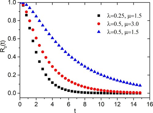
Table 4. The constant coefficients in Equation (Equation27(27)
(27) ) for the three parameter sets.
4.4. A circular repairable system
In this section, we study a circular repairable system. The state space is
, the set of working state is
and the set of failed states is
. The Q-matrix is
Suppose that all the eight components are working at time t, to evaluate the accuracy of the proposed method, we used the three parameter sets described in Section 4.3. Let i = 0 in Equation (Equation8
(8)
(8) ), we have
(28)
(28)
where
,
,…,
are constant coefficients and
,
,…,
are the non-zero eigenvalues of Q. Using the Q-matrix for each of the three parameter sets, the non-zero eigenvalues of Q are obtained and presented in Table .
Table 5. The non-zero eigenvalues of Q for three parameter sets.
Using the eigenvalues presented in Table for , we can obtain the constant coefficients in Equation (Equation28
(28)
(28) ) (see, Table ). When the values in Tables and are used in Equation (Equation28
(28)
(28) ), we plotted the reliability
against time t for the circular repairable
system in Figure based on the three parameter sets.
Figure 2. The plot of the reliability of the circular repairable
system against time t.
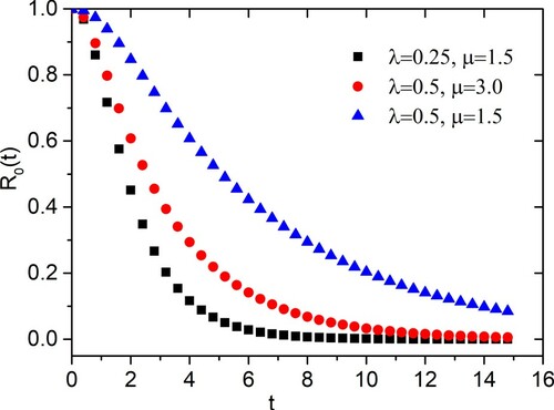
Table 6. The constant coefficients in Equation (Equation27(27)
(27) ) for the three parameter sets.
5. Concluding remarks
In this paper, a repairable system with n linearly and circularly arranged components is studied. A novel and simple method for determining the time-dependent transition performance probability and time-dependent reliability of the system when the state of the system is known within a certain of time is developed. Some numerical examples are used to illustrate the usefulness of the proposed method. Computer code written in R Core Team (Citation2019) to compute the time-dependent transition performance probability can be obtained from the authors upon request. The proposed method can serve as a simple alternative to the Laplace transform and the Runge-Kutta method which are commonly used to determine the time-dependent reliability of the repairable systems.
Disclosure statement
No potential conflict of interest was reported by the author(s).
Additional information
Funding
Notes on contributors
Gökhan Gökdere
Gökhan Gökdere is currently an Associate Professor of Statistical Science with the Fırat University, Elazıg, TURKEY. His research interests include reliability and statistical inference.
Hon Keung Tony Ng
Hon Keung Tony Ng is currently a Professor of Statistical Science with the Southern Methodist University, Dallas, TX, USA. His research interests include reliability, censoring methodology, ordered data analysis, nonparametric methods, and statistical inference. He is a Fellow of the American Statistical Association, an elected senior member of IEEE, and an elected member of the International Statistical Institute.
References
- Bollinger, R. C., & Salvia, A. A. (1982). Consecutive-k-out-of-n: F networks. IEEE Transactions on Reliability, R-31(1), 53–56. https://doi.org/https://doi.org/10.1109/TR.1982.5221227
- Chang, G. J., Cui, L. R., & Hwang, F. (2000). Reliabilities of consecutive-k-out-of-n:F systems. Kluwer.
- Cheng, K., & Zhang, Y. L. (2001). Analysis for a consecutive-k-out-of-n: F repairable system with priority in repair. International Journal of Systems Science, 32(5), 591–598. https://doi.org/https://doi.org/10.1080/00207720119474
- Chiang, D. T., & Niu, S. C. (1981). Reliability of consecutive-k-out-of-n:F system. IEEE Transactions on Reliability, R-30(1), 87–89. https://doi.org/https://doi.org/10.1109/TR.1981.5220981
- Derman, C., Lieberman, G. J., & Ross, S. M. (1982). On the consecutive-k-out-of-n:F system. IEEE Transactions on Reliability, R-31(1), 57–63. https://doi.org/https://doi.org/10.1109/TR.1982.5221229
- Eryilmaz, S. (2010). Review of recent advances in reliability of consecutive k-out-of-n and related systems. Proceedings of the Institution of Mechanical Engineers, Part O: Journal of Risk and Reliability, 224(3), 225–237. https://doi.org/https://doi.org/10.1243/1748006XJRR332
- Eryilmaz, S. (2014). Computing reliability indices of repairable systems via signature. Journal of Computational and Applied Mathematics, 260(2014), 229–235. https://doi.org/https://doi.org/10.1016/j.cam.2013.09.023
- Gökdere, G., Gürcan, M., & Kılıç, M. B. (2016). A new method for computing the reliability of consecutive k-out-of-n:F systems. Open Physics, 14(1), 166–170. https://doi.org/https://doi.org/10.1515/phys-2016-0015
- Guan, J., & Wu, Y. (2006). Repairable consecutive-k-out-of-n:F system with fuzzy states. Fuzzy Sets and Systems, 157(1), 121–142. https://doi.org/https://doi.org/10.1016/j.fss.2005.05.025
- Hongda, G., Lirong, C., & He, Y. (2019). Availability analysis of k-out-of-n:F repairable balanced systems with m sectors. Reliability Engineering and System Safety, 191(2019), 1–10. https://doi.org/https://doi.org/10.1016/j.ress.2019.106572
- Kontoleon, J. M. (1980). Reliability determination of a r-successive-out-of-n:F system. IEEE Transactions on Reliability, 29(5), 437. https://doi.org/https://doi.org/10.1109/TR.1980.5220921
- Kuo, W., & Zuo, M. (2003). Optimal reliability modeling: principles and applications. Wiley.
- Lam, Y., & Ng, H. K. T. (2001). A general model for consecutive-k-out-of-n: F repairable system with exponential distribution and (k−1)-step Markov dependence. European Journal of Operational Research, 129(3), 663–682. https://doi.org/https://doi.org/10.1016/S0377-2217(99)00474-9
- Lam, Y., & Zhang, Y. L. (1999). Analysis of repairable consecutive-2-out-of-n: F systems with Markov dependence. International Journal of Systems Science, 30(8), 799–809. https://doi.org/https://doi.org/10.1080/002077299291921
- Lam, Y., & Zhang, Y. L. (2000). Repairable consecutive-k-out-of-n:F system with Markov dependence. Naval Research Logistics (NRL), 47(1), 18–39. https://doi.org/https://doi.org/10.1002/(ISSN)1520-6750
- R Core Team (2019). R: A language and environment for statistical computing. R Foundation for Statistical Computing.
- Wang, G., Hu, L., Zhang, T., & Wang, Y. (2021). Reliability modeling for a repairable (k1,k2)-out-of-n: G system with phase-type vacation time. Applied Mathematical Modelling, 91(2), 311–321. https://doi.org/https://doi.org/10.1016/j.apm.2020.08.071
- Yam, R. C. M., Zuo, M. J., & Zhang, Y. L. (2003). A method for evaluation of reliability indices for repairable circular consecutive-k-out-of-n:F systems. Reliability Engineering and System Safety, 79(1), 1–9. https://doi.org/https://doi.org/10.1016/S0951-8320(02)00204-1
- Yuan, L., & Cui, Z. D. (2013). Reliability analysis for the consecutive-k-out-of-n: F system with repairmen taking multiple vacations. Applied Mathematical Modelling, 37(7), 4685–4697. https://doi.org/https://doi.org/10.1016/j.apm.2012.09.008
- Zhang, Y. L., & Lam, Y. (1998). Reliability of consecutive-k-out-of-n: G repairable system. International Journal of Systems Science, 29(12), 1375–1379. https://doi.org/https://doi.org/10.1080/00207729808929623
- Zhang, Y. L., & Wang, T. P. (1996). Repairable consecutive-2-out-of-n:F system. Microelectronics Reliability, 36(5), 605–608. https://doi.org/https://doi.org/10.1016/0026-2714(95)00183-2
- Zhang, Y. L., Wang, T. P., & Jia, J. S. (1998). Reliability analysis of consecutive-(n−1)-out-of-n:G repairable system. Chinese Journal of Automation, 10(1998), 181–186.
- Zhang, Y. L., Zuo, M. J., & Yam, R. C. M. (2000). Reliability analysis for a circular consecutive-2-out-of-n:F repairable system with priority in repair. Reliability Engineering and System Safety, 68(2), 113–120. https://doi.org/https://doi.org/10.1016/S0951-8320(99)00076-9
- Zuo, M. J., & Kuo, W. (1990). Design and performance analysis of consecutive-k-out-of-n structure. Naval Research Logistics, 37(2), 203–230. https://doi.org/https://doi.org/10.1002/(ISSN)1520-6750