Posterior contraction rate of sparse latent feature models with application to proteomics

Abstract

The Indian buffet process (IBP) and phylogenetic Indian buffet process (pIBP) can be used as prior models to infer latent features in a data set. The theoretical properties of these models are under-explored, however, especially in high dimensional settings. In this paper, we show that under mild sparsity condition, the posterior distribution of the latent feature matrix, generated via IBP or pIBP priors, converges to the true latent feature matrix asymptotically. We derive the posterior convergence rate, referred to as the contraction rate. We show that the convergence results remain valid even when the dimensionality of the latent feature matrix increases with the sample size, therefore making the posterior inference valid in high dimensional settings. We demonstrate the theoretical results using computer simulation, in which the parallel-tempering Markov chain Monte Carlo method is applied to overcome computational hurdles. The practical utility of the derived properties is demonstrated by inferring the latent features in a reverse phase protein arrays (RPPA) dataset under the IBP prior model.

Keywords:

• High dimension
• indian buffet process
• latent feature
• Markov chain monte carlo
• posterior convergence
• reverse phase protein arrays

1. Introduction

The latent feature models are concerned about finding latent structures in a data set $X_{n\times p}$ where each row ${\mathit{x}}_i=(x_{i1},\dots ,x_{ip})$ represents a single observation of p objects and n is the sample size. We consider the case where the number of objects $p=p_n$ increases as sample size n increases. The goal is to explain the variability of the observed data with a latent binary feature matrix $Z_{p\times K}$ where each column of Z represents a latent feature that includes a subset of the p objects. The number of latent features K is unknown and is inferred as well.

Bayesian nonparametric latent feature models such as the Indian buffet process (IBP) (Griffiths & Ghahramani, 2006, 2011) can be used to define the prior distribution of the binary latent feature matrix with arbitrarily many columns. In many applications (such as Chu et al., 2006) these priors could lead to desirable posterior inference. An important property of IBP is that the corresponding distribution maintains exchangeability across the rows that index the experimental units, making posterior inference relatively simple and easy to implement. However, sometimes the rows of the latent feature matrix must follow a group structure, such as in phylogenetic inferences. To address such needs, the phylogenetic Indian Buffet Process (pIBP) (Miller et al., 2008) has been developed to allow different rows to be partially exchangeable.

Despite the increasing popularity in the application of IBP and pIBP prior models, such as in cancer and evolutional genomics, few theoretical results have been discussed on the posterior inference based on these models. For example, from a frequentist view, it is important to investigate the asymptotic convergence of the posterior distribution of the latent feature matrix under IBP and pIBP priors. Existing literature on the theory of Bayesian posterior consistency includes, for example, Schwartz (1965), Barron et al. (1999) and Ghosal et al. (2000). Chen et al. (2016) is a motivational work exploring theoretical properties of the posterior distribution of the latent feature matrix based on IBP or pIBP priors. They explored the asymptotic behaviour of the IBP or pIBP-based posterior inference, where the sample size n increases in a much faster speed than the number of objects $p_n$, i.e., the dimensionality of Z. This might be hard to achieve in some real applications. We consider important extensions based on Chen et al. (2016). In particular, we consider properties of posterior inference based on IBP and pIBP priors in high dimensions and with sparsity. Under a similar high dimensional and sparse setting, related work is Pati et al. (2014), where the authors studied the asymptotic behaviour of sparse Bayesian factor models discussed in West (2003). These models are concerned about continuous latent features, which are different from the binary feature models like IBP and pIBP.

High dimensional inference is now routinely needed in many applications, such as genomics and proteomics. Due to the reduced cost of high-throughput biological experiments (e.g., next-generation sequencing), a number of genomics elements (such as genes) can be measured with a relatively short amount of time and low cost for a large number of patients. In our application, the number of genomics elements n is the sample size, the number of patients p is the number of rows, or the number of objects in the latent feature matrix, and the number of latent features K is assumed unknown. Depending on the particular research question, in some applications, genes can be the objects and patients can be the samples. When $p=p_n$ becomes large relative to n, the sparsity of the feature matrix critically ensures the efficiency and validity of statistical inference. We will show that under the sparsity condition, the requirement for posterior convergence can be relaxed from $p_n^3=o(n)$ (Chen et al., 2016) to $p_n(\log p_n{)}^2=o(n)$ (see Remark 3.2).

Our proposed sparsity condition can be expressed in terms of the number of features possessed by each object thus can be reasonably interpreted in practice. For example, in genomics and proteomics applications, our sparsity condition means that the number of features shared by different patients is small, i.e., the patients are heterogeneous. This is different from some published sparsity conditions that involve more complicated mathematical expressions, possibly in terms of the properties of complex matrices, which are difficult to check in real-world applications.

The rest of the paper is organized as follows. Section 2 introduces the latent feature model and the IBP/pIBP priors. Section 3 establishes the posterior contraction rate of sparse latent feature models under IBP and pIBP prior, which is the main theoretical result of this paper. Section 4 proposes an efficient posterior inference scheme based on Markov chain Monte Carlo (MCMC) simulations. Section 5 provides both simulated and real-world proteomics examples that support the theoretical derivations. We conclude the paper with a brief discussion in Section 6. Some technical details are provided in the supplement. The code for replicating the results reported in the manuscript can be accessed at https://github.com/tianjianzhou/IBP.

2. Notation and probability framework

In this section, we first introduce some notation, and then specify the hierarchical model including the sampling model and the prior model. In particular, the sampling model is the latent feature model, and the prior model is the IBP mixture or pIBP mixture.

2.1. Notation

Throughout the paper, we denote by $p(\cdot )$ and $P(\cdot )$ probability density functions (pdf) and probability mass functions (pmf), respectively. Specifically for the latent feature matrix Z, we use $\mathrm{\Pi }(Z)$ and $\mathrm{\Pi }(Z\mid X)$ to denote the prior and posterior distribution of Z, respectively. The likelihood $p(X\mid Z)=\prod _{i=1}^{n}p({\mathit{x}}_i^T\mid Z)$. For two sequences $a_n$ and $b_n$, the notation $a_n=O(b_n)$ means there exists a positive real number C and a constant $n_0$ such that $a_n\le C{b}_n$ for all $n\ge n_0$; the notation $a_n=o(b_n)$ means for every positive real number ε there exists a constant $n_0$ such that $a_n\le \epsilon b_n$ for all $n\ge n_0$. For a matrix A, $\Vert A\Vert$ denotes the spectral norm defined as the largest singular value of A. Finally, C is a generic notation for positive constants whose value might change depending on the context but is independent from other quantities.

2.2. Latent feature model

Suppose that $X_{n\times p}$ is a collection of the observed data. Each row ${\mathit{x}}_i=(x_{i1},\dots ,x_{ip})$ represents a single observation of p objects, for $i=1,\dots ,n$, where ${\mathit{x}}_i$'s are independent. Assume that the mechanism of generating X can be characterized by latent features, (1) $X^T=ZA+E.$(1) Here $Z=(z_{jk}{)}_{p\times K}$ denotes the latent binary feature matrix, each entry $z_{jk}\in \{0,1\}$ represents object j possesses feature k ($z_{jk}=1$) or not ($z_{jk}=0$), respectively. The loading matrix $A=(a_{ki}{)}_{K\times n}$, with each entry being the contribution of the k-feature to the ith observation. We assume $a_{ki}\stackrel{i.i.d}{\sim }N(0,{\sigma }_a^2)$. The error matrix $E=(e_{ji}{)}_{p\times n}$, where $e_{ji}$'s are independent Gaussian errors, $e_{ji}\stackrel{i.i.d}{\sim }N(0,{\sigma }^2)$.

After integrating out A, we obtain for each observation of the p objects, ${\mathit{x}}_i^T\stackrel{i.i.d}{\sim }{N}_p(\mathbf{0},{\sigma }_a^{2}Z{Z}^T+{\sigma }^2{\mathit{I}}_p),$ where $N_p$ is a p-variate Gaussian distribution. Therefore, the conditional distribution of X given Z is (2) $\begin{array}{rl}p(X\mid Z)& =\prod _{i=1}^n\frac{1}{\sqrt{(2\pi {)}^{p}det({\sigma }_a^{2}Z{Z}^T+{\sigma }^2{\mathit{I}}_p)}}\\ & \times \exp (-\frac{1}{2}{\mathit{x}}_i{({\sigma }_a^{2}Z{Z}^T+{\sigma }^2{\mathit{I}}_p)}^{-1}{\mathit{x}}_i^T).\end{array}$(2) Without loss of generality, following Chen et al. (2016), we always assume that ${\sigma }^2={\sigma }_a^2=1$ for deriving the theoretical results. One of the primary interests is to conduct appropriate estimation on $Z{Z}^T$, which is usually called the similarity matrix since each entry of $Z{Z}^T$ is the number of features shared by two objects.

2.3. Prior distributions based on IBP and pIBP

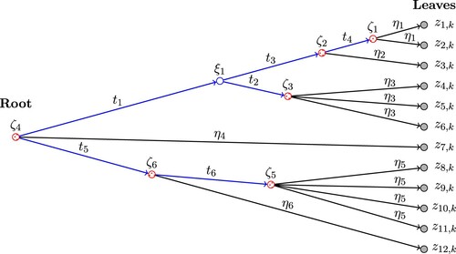
In the latent feature model (Equation (1(1) $X^T=ZA+E.$(1) )), it remains to specify the prior for the binary feature matrix Z. IBP and pIBP are popular prior choices on binary matrices with an unbounded number of columns. IBP assumes exchangeability among the objects, while pIBP introduces dependency among the entries of the kth column of Z through a rooted tree $\mathcal{T}$. See Figure 1 for an example of the tree. IBP is a special case of pIBP when the root node is the only internal node of the tree. The construction and the pmf of IBP are described and derived in detail in Griffiths and Ghahramani (2011). For pIBP, only a brief definition is given in Miller et al. (2008). For the proof of the main theoretical result of this paper, we propose a construction of pIBP in a similar way as IBP and derive the pmf of pIBP.

Figure 1. An example of a tree structure $\mathcal{T}$, which is a directed graph with random variables at the nodes (marked as circles). Entries of the kth column of Z, $z_{jk}$'s, are at the leaves. The lengths of all edges of $\mathcal{T}$, $t_i$'s and ${\eta }_l$'s, are marked on the figure. In particular, ${\eta }_l$'s represent the lengths between each leaf ($z_{jk}$, shaded nodes) and its parent node (${\zeta }_l$, dotted nodes). The total edge lengths $S(\mathcal{T})$ is the summation of the lengths of all edges of $\mathcal{T}$. In this example, $S(\mathcal{T})=\sum _{1\le i\le 6}{t}_i+(2{\eta }_1+{\eta }_2+3{\eta }_3+{\eta }_4+4{\eta }_5+{\eta }_6)$. The condition in case (2) of Lemma 3.3 in Section 3 means $\underset{1\le l\le 6}{inf}{\eta }_l\ge {\eta }_0$ for some ${\eta }_0>0$.

We first introduce some notation. Let ${\mathcal{Z}}_{p\times K}$ denote the collection of binary matrices with p rows and K ($K\in {\mathbb{N}}^{+}$) columns such that none of these columns consist of all 0's. Let ${\mathcal{Z}}_p={\cup }_{K=1}^{\mathrm{\infty }}{\mathcal{Z}}_{p\times K}$ and let $\mathbf{0}$ denote a p-dimensional vector whose elements are all 0's, i.e., $\mathbf{0}=(0,0,\dots ,0{)}^T.$ In the following sections, we also regard $\mathbf{0}$ as a $p\times 1$ matrix when needed. Both IBP and pIBP are defined over ${\mathcal{Z}}_p^0\triangleq \{\mathbf{0}\}\bigcup {\mathcal{Z}}_p$. It can be shown that with probability 1, a draw from IBP or pIBP has only finitely many columns. For the construction of IBP and pIBP, we introduce some more notations as follows. Denote by ${\tilde{\mathcal{Z}}}_{p\times \tilde{K}}$ the collection of all binary matrices with p rows and $\tilde{K}$ columns (where the columns can be all zeros). We define a many-to-one mapping $G(\cdot ):{\tilde{\mathcal{Z}}}_{p\times \tilde{K}}\to {\mathcal{Z}}_p^0$. For a binary matrix $\tilde{Z}\in {\tilde{\mathcal{Z}}}_{p\times \tilde{K}}$, if all columns of $\tilde{Z}$ are $\mathbf{0}$'s, then $G(\tilde{Z})=\mathbf{0}$; otherwise, $G(\tilde{Z})$ is obtained by deleting all zero columns of $\tilde{Z}$. For the purpose of performing inference on the similarity matrix $Z{Z}^T$, it suffices to focus on the set of equivalence classes induced by $G(\cdot )$. Two matrices ${\tilde{Z}}_1,{\tilde{Z}}_2\in {\tilde{\mathcal{Z}}}_{p\times \tilde{K}}$ are G-equivalent if $G({\tilde{Z}}_1)=G({\tilde{Z}}_2)$, and in this case the similarity matrices induced by ${\tilde{Z}}_1$ and ${\tilde{Z}}_2$ are the same, ${\tilde{Z}}_1{\tilde{Z}}_1^T={\tilde{Z}}_2{\tilde{Z}}_2^T$.

We now turn to a constructive definition of pIBP. The pIBP can be constructed in the following three steps by taking the limit of a finite feature model.

Step 1. Given some hyperparameter α and tree structure $\mathcal{T}$, we start by defining a probability distribution $P_{\tilde{K}}(\tilde{Z}\mid \alpha ,\mathcal{T})$ over $\tilde{Z}\in {\tilde{\mathcal{Z}}}_{p\times \tilde{K}}$. Denote by $\tilde{Z}=({\tilde{\mathit{z}}}_1,{\tilde{\mathit{z}}}_2,\dots ,{\tilde{\mathit{z}}}_{\tilde{K}})$. Let $\mathit{\pi }=\{{\pi }_1,{\pi }_2,\dots ,{\pi }_{\tilde{K}}\}$ be a vector of success probabilities such that $({\pi }_k\mid \alpha )\stackrel{i.i.d.}{\sim }\mathrm{Beta}(\alpha /\tilde{K},1)$. The columns of $\tilde{Z}$ are conditionally independent given $\mathit{\pi }$ and $\mathcal{T}$, $P_{\tilde{K}}(\tilde{Z}\mid \mathit{\pi },\mathcal{T})=\prod _{k=1}^{\tilde{K}}P({\tilde{\mathit{z}}}_k\mid {\pi }_k,\mathcal{T}),$ where $P({\tilde{\mathit{z}}}_k\mid {\pi }_k,\mathcal{T})$ is determined as in Miller et al. (2008) (more details in Supplementary Section S.1). If $P({\tilde{\mathit{z}}}_k\mid {\pi }_k,\mathcal{T})=\prod _{j=1}^{p}P({\tilde{z}}_{jk}\mid {\pi }_k)$ where ${\tilde{z}}_{jk}\stackrel{i.i.d}{\sim }\mathrm{Bernoulli}({\pi }_k)$, pIBP reduces to IBP. The marginal probability of $\tilde{Z}$ is $P_{\tilde{K}}(\tilde{Z}\mid \alpha ,\mathcal{T})=\prod _{k=1}^{\tilde{K}}\int P({\tilde{\mathit{z}}}_k\mid {\pi }_k,\mathcal{T})p({\pi }_k\mid \alpha )\mathrm{d}{\pi }_k.$

Step 2. Next, for any $Z\in {\mathcal{Z}}_p^0$ with K columns, we define a probability distribution (for $\tilde{K}\ge K$) ${\mathrm{\Pi }}_{\tilde{K}}(Z\mid \alpha ,\mathcal{T})\triangleq \sum _{\tilde{Z}\in {\tilde{\mathcal{Z}}}_{p\times \tilde{K}}:G(\tilde{Z})=Z}{P}_{\tilde{K}}(\tilde{Z}\mid \alpha ,\mathcal{T}),$ for $P_{\tilde{K}}(\tilde{Z}\mid \alpha ,\mathcal{T})$ defined in Step 1. That is, we collapse all binary matrices in ${\tilde{\mathcal{Z}}}_{p\times \tilde{K}}$ that are G-equivalent.

Step 3. Finally, for any $Z\in {\mathcal{Z}}_p^0$, define $\mathrm{\Pi }(Z\mid \alpha ,\mathcal{T})\triangleq \underset{\tilde{K}\to \mathrm{\infty }}{lim}{\mathrm{\Pi }}_{\tilde{K}}(Z\mid \alpha ,\mathcal{T}).$ Here $\mathrm{\Pi }(Z\mid \alpha ,\mathcal{T})$ is the pmf of pIBP under G-equivalence classes.

Based on the three steps of constructing pIBP, we derive the pmf of pIBP given α and $\mathcal{T}$. Details on the derivation is given in Supplementary Section S.1. Let $S(\mathcal{T})$ denote the total edge lengths of the tree structure (see Figure 1) and $\psi (\cdot )$ denote the digamma function. For $Z\in {\mathcal{Z}}_p^0$, we have (3) $\begin{array}{r}\mathrm{\Pi }(Z\mid \alpha ,\mathcal{T})=\{\begin{array}{l}\exp \{-(\psi (S(\mathcal{T})+1)-\psi (1))\alpha \},\\ \mathrm{if}Z=\mathbf{0};\\ {\displaystyle \exp \{-(\psi (S(\mathcal{T})+1)-\psi (1))\alpha \}}\\ \times {\displaystyle \frac{{\alpha }^K}{K!}\prod _{k=1}^K{\lambda }_k,\mathrm{if}Z\in {\mathcal{Z}}_{p\times K},}\end{array}\end{array}$(3) where ${\lambda }_k\triangleq \lambda ({\mathit{z}}_k,\mathcal{T})={\int }_0^{1}P({\mathit{z}}_k\mid {\pi }_k,\mathcal{T}){\pi }_k^{-1}\mathrm{d}{\pi }_k$ (See Supplementary Section S.1) and ${\mathit{z}}_k$ is the kth column of Z.

Assume $\alpha \sim \mathrm{Gamma}(1,1)$. After integrating out α, we obtain the pmf of pIBP mixture, $\begin{array}{r}\mathrm{\Pi }(Z\mid \mathcal{T})=\{\begin{array}{l}(\psi (S(\mathcal{T})+1)-\psi (1)+1{)}^{-1},\\ \mathrm{if}Z=\mathbf{0};\\ {\displaystyle (\psi (S(\mathcal{T})+1)-\psi (1)+1{)}^{-(K+1)}}\\ \times {\displaystyle \prod _{k=1}^K{\lambda }_k,\mathrm{if}Z\in {\mathcal{Z}}_{p\times K}.}\end{array}\end{array}$ For notational simplicity, we suppress the condition on $\mathcal{T}$ hereafter when we discuss pIBP.

When $S(\mathcal{T})=p$ and ${\lambda }_k={\int }_0^1\prod _{j=1}^p{\pi }_k^{m_k-1}(1-{\pi }_k{)}^{p-m_k}\mathrm{d}{\pi }_k$, pIBP reduces to IBP, where $m_k=\sum _{j=1}^p{z}_{jk}$ denotes the number of objects possessing feature k. The pmf of IBP mixture is $\mathrm{\Pi }(Z)=\{\begin{array}{l}(H_p+1{)}^{-1},\mathrm{if}Z=\mathbf{0};\\ {\displaystyle (H_p+1{)}^{-(K+1)}\prod _{k=1}^K\frac{(p-m_k)!(m_k-1)!}{p!},}\\ {\displaystyle \mathrm{if}Z\in {\mathcal{Z}}_{p\times K},}\end{array}$ where $H_p=\sum _{j=1}^p(1/j)$.

3. Posterior contraction rate under the sparsity condition

In this section, we establish the posterior contraction rate of IBP mixture and pIBP mixture under a sparsity condition. All the proofs are given in the supplement.

The sparsity condition is defined below for a sequence of binary matrices $\{Z_n^{\ast },n=1,2,\dots \}$.

Definition 3.1

Sparsity

Consider a sequence of binary matrices $\{Z_n^{\ast },n=1,2,\dots \}$ where $Z_n^{\ast }=(z_{jk}^{\ast }{)}_{p_n\times K_n^{\ast }}$. Assume that $m_{kn}\triangleq \sum _{j=1}^{p_n}{z}_{jk}^{\ast }\le s_n$ for some $s_n\ge 1$ and all $k=1,\dots ,K_n^{\ast }$. We say $\{Z_n^{\ast },n=1,2,\dots \}$ are sparse if $s_n/p_n\to 0$ as $n\to \mathrm{\infty }$.

The condition indicates that as sample size increases, the number of objects possessing any feature is upper-bounded and must be relatively small compared to the total number of objects. Therefore, such an assumption may be assessed via simulation studies and then applied to real-world applications. Examples will be provided later on. Similar but more strict assumptions are made in Castillo and van der Vaart (2012) and Pati et al. (2014), under different contexts.

Next, we review the definition of posterior contraction rate.

Definition 3.2

Posterior Contraction Rate

Let $\{Z_n^{\ast },n=1,2,\dots \}$ represent a sequence of true latent feature matrices where each $Z_n^{\ast }$ has $p_n$ rows. For each n, the observations are generated from ${\mathit{x}}_i^T\stackrel{i.i.d.}{\sim }N(0,Z_n^{\ast }{Z}_n^{\ast T}+{\mathit{I}}_{p_n})$ for $i=1,2,\dots ,n$. Denote by $\mathrm{\Pi }(\cdot \mid X)$ the posterior distribution of the latent feature matrix under IBP mixture or pIBP mixture prior. If $E_{Z_n^{\ast }}\left[\mathrm{\Pi }(\Vert Z_n{Z}_n^T-Z_n^{\ast }{Z}_n^{\ast T}\Vert \le C{ϵ}_n\mid X)\right]\to 1$ as $n\to \mathrm{\infty }$, where $\Vert \cdot \Vert$ represents the spectral norm and C is a positive constant, then we say the posterior contraction rate of $Z_n{Z}_n^T$ to the true $Z_n^{\ast }{Z}_n^{\ast T}$ is ${ϵ}_n$ under the spectral norm.

For the proof of the main theorem, we derive the following lemma. The lemma establishes the lower bound of $\mathrm{\Pi }(Z_n=Z_n^{\ast })$ for a sequence of binary matrices $\{Z_n^{\ast },n=1,2,\dots \}$ satisfying the sparsity condition, where $\mathrm{\Pi }(\cdot )$ represents the pmf of IBP mixture or pIBP mixture.

Lemma 3.3

Consider a sequence of binary matrices $\{Z_n^{\ast }:Z_n^{\ast }\in \{\mathbf{0}\}\bigcup {\mathcal{Z}}_{p_n\times K_n^{\ast }},n=1,2,\dots \}$ that are sparse under Definition 3.1. Parameters $m_{kn}$ and $s_n$ are defined accordingly (for $\mathbf{0}$ matrices, let $s_n=K_n^{\ast }=1$). We have $\mathrm{\Pi }(Z_n=Z_n^{\ast })\ge \exp (-C{s}_n{K}_n^{\ast }\log (p_n+1))$ for some positive constant C, if either of the following two cases is true: (1) $Z_n$ follows IBP mixture; (2) $Z_n$ follows pIBP mixture, and the minimal length between each leaf and its parent node is lower bounded by ${\eta }_0>0$ (see Figure 1).

Remark 3.1

Results in Lemma 3.3 depend on the sparsity condition. As a counterexample, we approximate $\mathrm{\Pi }(Z_n=Z_n^{\ast })$ for a sequence of non-sparse binary matrices $\{Z_n^{\ast },n=1,2,\dots \}$, where $Z_n^{\ast }\in {\mathcal{Z}}_{p_n}$, and $Z_n$ follows IBP mixture. Recall that for IBP mixture, we have $\begin{array}{rl}\mathrm{\Pi }(Z_n=Z_n^{\ast })& =\frac{1}{(H_{p_n}+1{)}^{K_n^{\ast }+1}}\prod _{k=1}^{K_n^{\ast }}\\ & \times \frac{(p_n-m_{kn})!(m_{kn}-1)!}{p_n!}.\end{array}$ Let $m_{kn}=p_n/2$ for every column $k=1,\dots ,K_n^{\ast }$, then $[(p_n-m_{kn})!(m_{kn}-1)!]/(p_n!)=[(p_n/2)!(p_n/2-1)!]/(p_n!)$ and Stirling's formula implies that $[(p_n/2)!(p_n/2-1)!]/(p_n!)\sim \sqrt{2\pi /p_n}{2}^{-p_n}$. Since $H_{p_n}=\log p_n+O(1)$, $\begin{array}{rl}\mathrm{\Pi }(Z_n& =Z_n^{\ast })\le \exp (-C{K}_n^{\ast }\log \log (p_n+2))\\ & \times {\left(C\sqrt{\frac{2\pi }{p_n}}\frac{1}{2^{p_n}}\right)}^{K_n^{\ast }}\le \exp (-C{K}_n^{\ast }{p}_n).\end{array}$ Comparing the results obtained with and without sparsity conditions, we find the lower-bound with sparsity condition is very likely to be larger than the upper-bound without sparsity condition. To consider a very extreme case, when $s_n=\log (p_n+1)$, the lower-bound $\exp (-C{K}_n^{\ast }(\log (p_n+1){)}^2)$ is much larger than $\exp (-C{K}_n^{\ast }{p}_n)$.

We present the main theorem of this paper, which proves that for a sequence of true latent feature matrix $Z_n^{\ast }$ that satisfy the sparsity condition in Definition 3.1, the posterior distribution of the similarity matrix $Z_n{Z}_n^T$ converges to $Z_n^{\ast }{Z}_n^{\ast T}$. The theorem eventually leads to the main theoretical result in Remark 3.2 later.

Theorem 3.4

Consider a sequence of sparse binary matrices $\{Z_n^{\ast },n=1,2,\dots \}$ as in Definition 3.1 and the prior in either of the two cases of Lemma 3.3. For each n, suppose the observations are generated from ${\mathit{x}}_i^T\stackrel{i.i.d.}{\sim }N(0,Z_n^{\ast }{Z}_n^{\ast T}+{\mathit{I}}_{p_n})$ for $i=1,2,\dots ,n$. Let $\begin{array}{rl}{ϵ}_n& =\frac{max\{\sqrt{p_n},\sqrt{s_n{K}_n^{\ast }\log (p_n+1)}\}}{\sqrt{n}}\\ & \times max\{1,\Vert Z_n^{\ast }{Z}_n^{\ast T}\Vert \}.\end{array}$ If ${ϵ}_n\to 0$ as $n\to \mathrm{\infty }$, then we have $E_{Z_n^{\ast }}\left[\mathrm{\Pi }(\Vert Z_n{Z}_n^T-Z_n^{\ast }{Z}_n^{\ast T}\Vert \le C{ϵ}_n\mid X)\right]\to 1$ as $n\to \mathrm{\infty }$ for some positive constant C. In other words, ${ϵ}_n$ is the posterior contraction rate under the spectral norm.

For the sequence of sparse binary matrices $\{Z_n^{\ast },n=1,2,\dots \}$ considered in Theorem 3.4, if $\Vert Z_n^{\ast }{Z}_n^{\ast T}\Vert \le M_n$ for some $M_n\ge 1$ and ${\widetilde{ϵ}}_n\triangleq \frac{max\{\sqrt{p_n},\sqrt{s_n{K}_n^{\ast }\log (p_n+1)}\}}{\sqrt{n}}{M}_n\to 0$ as $n\to \mathrm{\infty }$, then ${\widetilde{ϵ}}_n$ is a valid posterior contraction rate. We show in the following corollary that if the number of features possessed by each object is upper bounded, then a new posterior contraction rate with a simpler expression (compared to Theorem 3.4) can be derived.

Corollary 3.5

Consider a sequence of sparse binary matrices $\{Z_n^{\ast },n=1,2,\dots \}$ as in Definition 3.1 where $Z_n^{\ast }=(z_{jk}^{\ast }{)}_{p_n\times K_n^{\ast }}$. Suppose that there exists $q_n\ge 1$ such that $\underset{1\le j\le p_n}{sup}\left(\sum _{k=1}^{K_n^{\ast }}{z}_{jk}^{\ast }\right)\le q_n,$ i.e., the number of features possessed by each object (non-zero entries of each row of $Z_n^{\ast }$) is upper bounded by $q_n$. Given the same assumptions as in Theorem 3.4 except for replacing ${ϵ}_n\to 0$ by ${\widetilde{ϵ}}_n\triangleq \frac{max\{\sqrt{p_n},\sqrt{s_n{K}_n^{\ast }\log (p_n+1)}\}}{\sqrt{n}}{s}_n{q}_n\to 0$ as $n\to \mathrm{\infty }$, we have $E_{Z_n^{\ast }}\left[\mathrm{\Pi }(\Vert Z_n{Z}_n^T-Z_n^{\ast }{Z}_n^{\ast T}\Vert \le C{\widetilde{ϵ}}_n\mid X)\right]\to 1$ as $n\to \mathrm{\infty }$ for some positive constant C. Specifically,

(1)	if there is no additional condition on $q_n$, ${\widetilde{ϵ}}_n=\frac{max\{\sqrt{p_n},\sqrt{s_n{K}_n^{\ast }\log (p_n+1)}\}}{\sqrt{n}}{s}_n{K}_n^{\ast };$
(2)	if $q_n$ is a constant, ${\widetilde{ϵ}}_n=\frac{max\{\sqrt{p_n},\sqrt{s_n{K}_n^{\ast }\log (p_n+1)}\}}{\sqrt{n}}{s}_n.$

Remark 3.2

Consider the second case of Corollary 3.5. If (1) $s_n{K}_n^{\ast }\log (p_n+1)=O(p_n)$ and (2) $s_n=O(\log (p_n+1))$, then ${\widetilde{ϵ}}_n\le C\frac{\sqrt{p_n}\log (p_n+1)}{\sqrt{n}}$; therefore, if $p_n(\log (p_n+1){)}^2=o(n)$, then $\frac{\sqrt{p_n}\log (p_n+1)}{\sqrt{n}}$ is a valid posterior contraction rate. In other words, to ensure posterior convergence, we only need n to increase a little bit faster than $p_n$, given the assumptions (1), (2) and the condition in the second case of Corollary 3.5.

4. Posterior inference based on MCMC

We have specified the hierarchical models including the sampling model $p(X\mid Z)$ and the prior models for the parameters $\mathrm{\Pi }(Z\mid \alpha )$ and $p(\alpha )$. In particular, $p(X\mid Z)$ is the latent feature model (Equation (2(2) $\begin{array}{rl}p(X\mid Z)& =\prod _{i=1}^n\frac{1}{\sqrt{(2\pi {)}^{p}det({\sigma }_a^{2}Z{Z}^T+{\sigma }^2{\mathit{I}}_p)}}\\ & \times \exp (-\frac{1}{2}{\mathit{x}}_i{({\sigma }_a^{2}Z{Z}^T+{\sigma }^2{\mathit{I}}_p)}^{-1}{\mathit{x}}_i^T).\end{array}$(2) )), $\mathrm{\Pi }(Z\mid \alpha )$ is the IBP or pIBP prior (Equation (3(3) $\begin{array}{r}\mathrm{\Pi }(Z\mid \alpha ,\mathcal{T})=\{\begin{array}{l}\exp \{-(\psi (S(\mathcal{T})+1)-\psi (1))\alpha \},\\ \mathrm{if}Z=\mathbf{0};\\ {\displaystyle \exp \{-(\psi (S(\mathcal{T})+1)-\psi (1))\alpha \}}\\ \times {\displaystyle \frac{{\alpha }^K}{K!}\prod _{k=1}^K{\lambda }_k,\mathrm{if}Z\in {\mathcal{Z}}_{p\times K},}\end{array}\end{array}$(3) )) and $p(\alpha )=\mathrm{Gamma}(1,1)$. For the theoretical results in Section 3, we integrate out α. For posterior inference, we keep α so that the conditional distributions can be obtained in closed form.

We use Markov chain Monte Carlo simulations to generate samples from the posterior $(Z,\alpha )\sim \mathrm{\Pi }(Z,\alpha \mid X)\propto p(X\mid Z)\mathrm{\Pi }(Z\mid \alpha )p(\alpha )$. After iterating sufficiently many steps, the samples of Z drawn from the Markov chain approximately follow $\mathrm{\Pi }(Z\mid X)$. Gibbs sampling transition probabilities can be used to update Z and α, as described in Griffiths and Ghahramani (2011) and Miller et al. (2008).

To overcome trapping of the Markov chain in local modes in the high-dimensional setting, we use parallel tempering Markov chain Monte Carlo (PTMCMC) (Geyer, 1991) in which several Markov chains at different temperatures run in parallel and interchange the states across each other. In particular, the target distribution of the Markov chain indexed by temperature T is ${\mathrm{\Pi }}^{(T)}(Z,\alpha \mid X)\propto p(X\mid Z{)}^{\frac{1}{T}}\mathrm{\Pi }(Z\mid \alpha )p(\alpha ).$ Parallel tempering helps the original Markov chain (the Markov chain whose temperature T is 1) avoid getting stuck in local modes and approximate the target distribution efficiently.

We give an algorithm below for sampling from $\mathrm{\Pi }(Z,\alpha \mid X)$ where $\mathrm{\Pi }(Z\mid \alpha )$ follows IBP. The algorithm describes in detail how PTMCMC can be combined with the Gibbs sampler in Griffiths and Ghahramani (2011). The algorithm iterates Steps 1 and 2 in turn.

Step 1 (Updating Z and α). Denote by $z_{jk}$ the entries of Z, $j=1,\dots ,p$ and $k=1,\dots ,K$. We update Z by row. For each row j, we iterate through the columns $k=1,\dots ,K$. We first make a decision to drop the kth column of Z, ${\mathit{z}}_k$, if and only if $m_{(-j)k}=\sum _{j^{\prime }\ne j}{z}_{j^{\prime }k}=0$. In other words, if feature k is not possessed by any object other than j, then the kth column of Z should be dropped, regardless of whether $z_{jk}=0$ or 1.

If the kth column is not dropped, we sample $z_{jk}$ from ${\mathrm{\Pi }}^{(T)}(z_{jk}\mid \dots )\propto p(X\mid Z{)}^{\frac{1}{T}}\mathrm{\Pi }(z_{jk}\mid Z_{(-jk)},\alpha ),$ where $Z_{(-jk)}$ represents all entries of Z except $z_{jk}$ and $P(X\mid Z)$ is determined by ${\mathit{x}}_i^T\mid Z\stackrel{i.i.d.}{\sim }N(0,Z{Z}^T+{\mathit{I}}_p)$, in which ${\mathit{x}}_i$'s are rows of X. The conditional prior $\mathrm{\Pi }(z_{jk}\mid Z_{(-jk)},\alpha )$ only depends on ${\mathit{z}}_{(-j)k}$ (i.e., the kth column of Z excluding $z_{jk}$). Specifically, $\mathrm{\Pi }(z_{jk}=1\mid Z_{(-jk)},\alpha )=\frac{m_{(-j)k}}{p}.$ After updating all entries in the jth row, we add a random number of $K_j^{+}$ columns (features) to Z. The $K_j^{+}$ new features are only possessed by object j, i.e., only the jth entry is 1 while all other entries are 0. Let $Z_{+}$ denote the feature matrix after $K_j^{+}$ columns are added to the old feature matrix. The conditional posterior distribution of $K_j^{+}$ is $P^{(T)}(K_j^{+}\mid \dots )\propto p(X\mid Z_{+}{)}^{\frac{1}{T}}P(K_j^{+}\mid \alpha ),$ in which $P(K_j^{+}\mid \alpha )$ is the prior distribution of $K_j^{+}$ under IBP, $P(K_j^{+}\mid \alpha )=\mathrm{Pois}(\alpha /p)$. The support of $P^{(T)}(K_j^{+}\mid \dots )$ is $\mathbb{N}$. For easier evaluation of $P^{(T)}(K_j^{+}\mid \dots )$, we work with an approximation by truncating $P^{(T)}(K_j^{+}\mid \dots )$ at level $K_{max}^{+}$, similar to the idea of truncating a stick-breaking prior in Ishwaran and James (2001). The value $K_{max}^{+}$ is the maximum number of new columns (features) that can be added to Z each time we update the jth row. Denote by ${\tilde{P}}^{(T)}(K_j^{+}\mid \dots )$ the truncated conditional posterior, we have (4) $\begin{array}{rl}{\tilde{P}}^{(T)}(K_j^{+}& =k\mid \dots )=\frac{P^{(T)}(k\mid \dots )}{\sum _{k^{\prime }=0}^{K_{max}^{+}}{P}^{(T)}(k^{\prime }\mid \dots )},\\ & \mathrm{for}k=0,1,\dots ,K_{max}^{+}.\end{array}$(4) Lastly, we update α. Given Z, the observed data X and α are conditionally independent, which implies that the conditional posterior distribution of α at any temperature T is the same. We sample α from $(\alpha \mid \dots )\sim \mathrm{Gamma}(K+1,{(\sum _{j=1}^p\frac{1}{j}+1)}^{-1}).$

Step 2 (Interchanging States across Parallel Chains). We sort the Markov chains in descending order by their temperatures T. The next step of PTMCMC is interchanging states between adjacent Markov chains. Let $(Z^{(T)},{\alpha }^{(T)})$ denote the state of the Markov chain indexed by temperature T. Suppose we run N parallel chains with descending temperatures $T_N,T_{N-1},\dots ,T_2,T_1$, where $T_1=1$. Sequentially for each $i=N,N-1,\dots ,2$, we propose an interchange of states between $(Z^{(T_i)},{\alpha }^{(T_i)})$ and $(Z^{(T_{i-1})},{\alpha }^{(T_{i-1})})$ and accept the proposal with probability $A_{T_i,T_{i-1}}=min\{{\left(\frac{p(X\mid Z^{(T_{i-1})})}{p(X\mid Z^{(T_i)})}\right)}^{\frac{1}{T_i}-\frac{1}{T_{i-1}}},1\}.$

5. Examples

5.1. Simulation studies

We conduct simulation to examine the convergence of the posterior distribution of $Z_n{Z}_n^T$ (under IBP mixture prior) to the true similarity matrix $Z_n^{\ast }{Z}_n^{\ast T}$. We consider several true similarity matrices with different sample sizes n's and explore the contraction of the posterior distribution. Hereinafter, we suppress the index n.

5.1.1. Simulations under the sparsity condition of $Z^{\ast }$

In this simulation, the true latent feature matrix, $Z^{\ast }=(z_{jk}^{\ast }{)}_{p\times K^{\ast }}$, is randomly generated under the sparsity condition in Definition 3.1 (i.e., $m_k\le s$ for $k=1,\dots ,K^{\ast }$, where s is relatively small compared with p). We set s = 10, $K^{\ast }=10$ and $p=50,100,$ or 150. We use s/p to measure the sparsity (as in Definition 3.1).

Once $Z^{\ast }$ is generated, the samples ${\mathit{x}}_1,{\mathit{x}}_2,\dots ,{\mathit{x}}_n$ are generated under the sampling model (Equation (2(2) $\begin{array}{rl}p(X\mid Z)& =\prod _{i=1}^n\frac{1}{\sqrt{(2\pi {)}^{p}det({\sigma }_a^{2}Z{Z}^T+{\sigma }^2{\mathit{I}}_p)}}\\ & \times \exp (-\frac{1}{2}{\mathit{x}}_i{({\sigma }_a^{2}Z{Z}^T+{\sigma }^2{\mathit{I}}_p)}^{-1}{\mathit{x}}_i^T).\end{array}$(2) )) with ${\mathit{x}}_i^T\stackrel{i.i.d.}{\sim }N(0,Z^{\ast }{Z}^{\ast T}+{\mathit{I}}_p),$ where ${\mathit{x}}_i$'s are rows of X. For each value of p, we conduct 4 simulations, with sample sizes n = 20, 50, 80 or 100.

Given simulated data X, we use the proposed PTMCMC algorithm introduced in Section 4 to sample from the posterior distribution $\mathrm{\Pi }(Z\mid X)$, setting $K_{max}^{+}$ in (4(4) $\begin{array}{rl}{\tilde{P}}^{(T)}(K_j^{+}& =k\mid \dots )=\frac{P^{(T)}(k\mid \dots )}{\sum _{k^{\prime }=0}^{K_{max}^{+}}{P}^{(T)}(k^{\prime }\mid \dots )},\\ & \mathrm{for}k=0,1,\dots ,K_{max}^{+}.\end{array}$(4) ) at 10. We set the number of parallel Markov chains N = 11 with geometrically spaced temperatures. Namely, the ratio between adjacent temperatures $\beta \triangleq T_{i+1}/T_i=1.2$, with $T_1=1$. We run 1000 MCMC iterations. The chains converge quickly and mix well based on basic MCMC diagnostics.

We repeat the simulation scheme 40 times, each time generating a new data set with a new random seed and applying the PTMCMC algorithm for inference. We report several summaries in Table 1 based on the 40 simulation studies. The entries are the true values of $(n,p)$ (first column), p/n (second column), average (across the 40 simulation studies) of the 1000th MCMC value of K (third column), average residual $\Vert Z{Z}^T-Z^{\ast }{Z}^{\ast T}\Vert$ based on the 1000th MCMC value of Z (fourth column), average ϵ value as defined in Theorem 3.4 (fifth column), and average $\Vert Z{Z}^T-Z^{\ast }{Z}^{\ast T}\Vert /ϵ$ value (sixth column).

Table 1. Simulation results for different combinations of n and p.

$(n,p)$	p/n	$K_{sd}$	$\Vert Z{Z}^T-Z^{\ast }{Z}^{\ast T}{\Vert }_{sd}$	${ϵ}_{sd}$	$(\Vert Z{Z}^T-Z^{\ast }{Z}^{\ast T}\Vert /ϵ{)}_{sd}$
$(20,50)$	2.5	${13.550}_{2.385}$	${16.349}_{5.315}$	${125.191}_{6.627}$	${0.131}_{0.043}$
$(50,50)$	1	${10.700}_{0.791}$	$\phantom{1}{3.444}_{2.205}$	$\phantom{1}{79.178}_{4.191}$	${0.043}_{0.027}$
$(80,50)$	0.625	${10.300}_{0.564}$	$\phantom{1}{0.591}_{1.117}$	$\phantom{1}{62.596}_{3.313}$	${0.009}_{0.018}$
$(100,50)$	0.5	${10.275}_{0.506}$	$\phantom{1}{0.478}_{0.951}$	$\phantom{1}{55.987}_{2.964}$	${0.008}_{0.017}$
$(20,100)$	5	${12.650}_{1.718}$	${12.505}_{3.029}$	$\phantom{1}{92.532}_{7.750}$	${0.136}_{0.032}$
$(50,100)$	2	${10.750}_{0.776}$	$\phantom{1}{3.495}_{1.552}$	$\phantom{1}{58.522}_{4.901}$	${0.060}_{0.027}$
$(80,100)$	1.25	${10.275}_{0.506}$	$\phantom{1}{0.709}_{1.315}$	$\phantom{1}{46.266}_{3.875}$	${0.016}_{0.030}$
$(100,100)$	1	${10.250}_{0.494}$	$\phantom{1}{0.343}_{0.734}$	$\phantom{1}{41.382}_{3.466}$	${0.008}_{0.017}$
$(20,150)$	7.5	${12.600}_{2.073}$	$\phantom{1}{11.339}_{2.618}$	$\phantom{1}{84.131}_{5.881}$	${0.136}_{0.036}$
$(50,150)$	3	${10.675}_{0.797}$	$\phantom{1}{3.387}_{1.876}$	$\phantom{1}{53.209}_{3.719}$	${0.063}_{0.033}$
$(80,150)$	1.875	${10.282}_{0.456}$	$\phantom{1}{0.472}_{0.884}$	$\phantom{1}{42.065}_{2.940}$	${0.012}_{0.022}$
$(100,150)$	1.5	${10.250}_{0.439}$	$\phantom{1}{0.250}_{0.439}$	$\phantom{1}{37.624}_{2.630}$	${0.007}_{0.012}$

Note: The true $K^{\ast }=10$. Results are based on the sample values of K and Z from the 1000th MCMC iteration. The ϵ values are calculated based on the definition in Theorem 3.4. Entries in normal size and in the subscript (columns 3 and 4) are the averages and standard deviations over 40 independent simulation studies.

For fixed p, $Z{Z}^T$ converges to $Z^{\ast }{Z}^{\ast T}$ as sample size increases. When n = 100, $\Vert Z{Z}^T-Z^{\ast }{Z}^{\ast T}\Vert$ is very close to 0 and K is close to the truth $K^{\ast }=10$. On the other hand, for fixed n, increasing p does not make the posterior distribution of $Z{Z}^T$ significantly less concentrated at the true $Z^{\ast }{Z}^{\ast T}$, implying that the inference is robust to high-dimensional matrix of Z as long as the true matrix $Z^{\ast }$ is sparse. 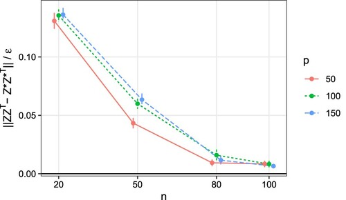The value of $\Vert Z{Z}^T-Z^{\ast }{Z}^{\ast T}\Vert /ϵ$ demonstrates the convergence result in Theorem 3.4. As shown in Figure 2, as sample size increases, $\Vert Z{Z}^T-Z^{\ast }{Z}^{\ast T}\Vert /ϵ$ converges to 0. This verifies the theoretical results we have reported early on. Note that similar to Chen et al. (2016), we use $\Vert Z{Z}^T-Z^{\ast }{Z}^{\ast T}\Vert /ϵ$ instead of the probability $\mathrm{\Pi }(\Vert Z{Z}^T-Z^{\ast }{Z}^{\ast T}\Vert \le Cϵ\mid X)$ to demonstrate the theoretical results due to the arbitrariness of the constant term C. With a finite number of simulation experiments, one can always find a constant C such that $\mathrm{\Pi }(\Vert Z{Z}^T-Z^{\ast }{Z}^{\ast T}\Vert \le Cϵ\mid X)$ is always 1.

Figure 2. Simulation results for different combinations of n and p. Plot of $\Vert Z_n{Z}_n^T-Z_n^{\ast }{Z}_n^{\ast T}\Vert /{ϵ}_n$ versus n, where $\Vert Z_n{Z}_n^T-Z_n^{\ast }{Z}_n^{\ast T}\Vert$ is the spectral norm for the residual of the similarity matrix, and ${ϵ}_n$ is the posterior contraction rate defined in Theorem 3.4. The ratio converges to zero as n increases, demonstrating the theoretical results. The vertical error bars represent one standard error.

5.1.2. Sensitivity of sparsity

In this part, we use simulation results to demonstrate the effect of sparsity of $Z^{\ast }$ in the posterior convergence. We set p = 50, $K^{\ast }=10$ and n = 100, and use different $s=10,15,18,20,23,25$, reducing the sparsity of $Z^{\ast }$ gradually. We generate $Z^{\ast }$ and X the same way as in the previous simulation. We set the number of parallel Markov chains N = 11 and $K_{max}^{+}=10$. To increase the frequency of interchange between adjacent chains, we reduce β to 1.15.

Table 2 reports the simulation results. As $Z^{\ast }$ becomes less sparse, the posterior distribution of Z becomes less concentrated on $Z^{\ast }$, in terms of both K and $\Vert Z{Z}^T-Z^{\ast }{Z}^{\ast T}\Vert$. Specifically, for $s\in \{15,20,25\}$, when s increases by 5, $\Vert Z{Z}^T-Z^{\ast }{Z}^{\ast T}\Vert$ inflates more than 10 fold.

Table 2. Simulation results for different s.

s	s/p	$K_{sd}$	$\Vert Z{Z}^T-Z^{\ast }{Z}^{\ast T}{\Vert }_{sd}$
10	0.2	${10.225}_{0.480}$	${0.200}_{0.405}$
15	0.3	${10.100}_{0.304}$	${0.100}_{0.304}$
18	0.36	${10.225}_{0.423}$	${1.212}_{5.454}$
20	0.4	${10.275}_{0.554}$	${1.959}_{5.146}$
23	0.46	${10.850}_{0.802}$	${20.192}_{26.867}$
25	0.5	${11.150}_{0.736}$	${24.552}_{19.141}$

Note: The true $(n,p,K^{\ast })=(100,50,10)$. Results are based on the sample values of K and Z from the 1000th MCMC iteration. Entries in normal size and in the subscript (rows 3 and 4) are the averages and standard deviations over 40 independent simulation studies.

5.2. Application for proteomics

We apply the binary latent feature model to the analysis of a reverse phase protein arrays (RPPA) dataset from The Cancer Genome Atlas (TCGA, https://tcga-data.nci.nih.gov/tcga/) downloaded by TCGA Assembler 2 (Wei et al., 2017). The RPPA dataset records the levels of protein expression based on incubating a matrix of biological samples on a microarray with specific antibodies that target corresponding proteins (Sheehan et al., 2005; Spurrier et al., 2008). We focus on patients categorized as 5 different cancer types, including breast cancer (BRCA), diffuse large B-cell lymphoma (DLBC), glioblastoma multiforme (GBM), clear cell kidney carcinoma (KIRC) and lung adenocarcinoma (LUAD). Data of n = 157 proteins from p = 100 patients are available, with an equal number of 20 patients for each cancer type. Note that we consider proteins as experimental units and patients as objects in the data matrix with an aim to allocate latent features to patients (not proteins). This will be clear later when we report the inference results. The rows of the data matrix $X_{n\times p}$ are standardized, with $\sum _{j=1}^p{x}_{ij}=0$ for $i=1,\dots ,n$. Since the patients are from different cancer types, we expect the data to be highly heterogeneous and the number of common features that two patients share to be small, i.e the feature matrix is sparse.

We fit the binary latent feature model under the IBP prior $\mathrm{\Pi }(Z\mid \alpha )$ and $\alpha \sim \mathrm{Gamma}(1,1)$. In addition, rather than fixing ${\sigma }^2={\sigma }_a^2=1$, we now assume inverse-Gamma distribution priors on them, ${\sigma }^2\sim \mathrm{IG}(1,1)$ and ${\sigma }_a^2\sim \mathrm{IG}(1,1)$. We run 1,000 MCMC iterations, as in the simulation studies. We also repeat the MCMC algorithm 3 times with different random seeds and do not observe substantial difference across the runs. 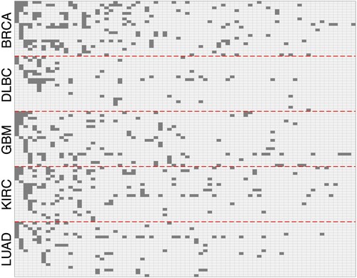We report point estimates $(\hat{Z},\hat{\alpha },{\hat{\sigma }}^2,{\hat{\sigma }}_a^2)$ according to the maximum a posteriori (MAP) estimate, $(\hat{Z},\hat{\alpha },{\hat{\sigma }}^2,{\hat{\sigma }}_a^2)=\underset{(Z,\alpha ,{\sigma }^2,{\sigma }_a^2)}{\arg \max }p(Z,\alpha ,{\sigma }^2,{\sigma }_a^2\mid X).$ Figure 3 shows the inferred binary feature matrix $\hat{Z}$, where a shaded gray rectangle indicates the corresponding patient j possesses feature k. For the real data analysis we do not know the true latent feature matrix and its sparsity, but can use the estimated $\hat{Z}$ to approximate the truth. From the $\hat{Z}$ matrix, we find that a feature is possessed by at most $\hat{s}=31$ patients, and therefore the sparsity of $\hat{Z}$ is about $\hat{s}/p=0.31$. If the estimated sparsity is close to the truth, according to simulation results (Section 5.1 Table 2), the posterior distribution of Z should be highly concentrated at the truth $Z^{\ast }$.

Figure 3. The inferred binary feature matrix $\hat{Z}$ for the TCGA RPPA dataset. The dataset consists of 100 patients, with 20 patients for each of the 5 cancer type, BRCA, DLBC, GBM, KIRC and LUAD. A shaded gray rectangle indicates the corresponding patient j possesses feature k, i.e., the corresponding matrix element ${\hat{Z}}_{jk}=1$. The columns are in descending order of the number of objects possessing each feature. The rows are reordered for better display.

5.2.1. Biological interpretation of the features

We report the unique genes for the top 10 proteins that have the largest loading values ${\hat{a}}_{ki}$ for the five most popular features. That is, for the top five features k possessed by the largest numbers of patients (the first five columns in Figure 3), we report the proteins with the largest ${\hat{a}}_{ki}$ values. The ${\hat{a}}_{ki}$ values are posterior mean from the MCMC samples, in which parameters $a_{ki}$'s are sampled from their full conditional distributions. This additional sampling step for $a_{ki}$'s is added to the proposed PTMCMC algorithm for the purpose of assessing the biological implication of the features. It is a simple Gibbs step as the full conditional distributions of $a_{ki}$'s are known Gaussian distributions. Table S.1 in the supplement lists these genes and their feature membership. We conduct the gene set enrichment analysis (GSEA) in Subramanian et al. (2005) comparing the genes in each feature with pathways from the Kyoto Encyclopedia of Genes and Genomes (KEGG) database (Kanehisa & Goto, 2000). The GSEA analysis reports back the enriched pathways and the corresponding genes, which is listed in Table S.2 in the supplement. We observe the following findings.

Feature 1. Among all the features, only genes in feature 1 are enriched in the cell cycle pathway. They are also enriched in the p53 signaling pathway. This indicates that feature 1 might be related to cell death and cell cycle. Feature 2. Feature 2 is enriched in many different types of pathways, which may be caused by its two key gene members: NRAS:4893 (oncogene) and PTEN:5728 (tumor suppressor). These two genes play key roles in the PI3K-Akt signaling pathway and also regulate many other cancer-related pathways. Feature 3. Genes in feature 3 are enriched in inflammation related pathways, such as the non-alcoholic fatty liver disease, Hepatitis B, viral carcinogenesis, hematopoietic cell lineage and phagosome pathways. This means feature 3 is mostly related to inflammation. Feature 4 and 5. Genes in features 4 and 5 are enriched in the largest number of pathways that are similar, with the exception of the p53 pathway (enriched with feature 4 but not 5) and the Jak-STAT signaling pathway (enriched with feature 5 but not 4). This indicates that feature 4 is more related to intracellular factors like DNA damage, oxidative stress and activated oncogenes, while feature 5 is more related to extracellular factors such as cytokines and growth factors.

Depending on the possession of the first five features, the patients in each cancer type can be further divided into potential molecular subgroups. For example, most BRCA patients possess features 1, 2 or 3, which indicate that these tumours are related to cell death and cell cycle (features 1 & 2), or inflammation (feature 3) pathways; most of the GBM and KIRC patients possess features 1, 2, 3 or 4, indicating an additional subgroup of patients with tumour associated to DNA damage (feature 4). The DLBC patients are highly heterogeneous, as many of them do not possess any of the first five main features. This has been well recognized in the literature (Zhang et al., 2013). Lastly, LUAD seems to have two subgroups, possessing mostly feature 1 or 2, respectively. They correspond to cell death and cell cycle functions, which suggest that these two subgroups of cancer could be related to abnormal cell death and cell cycle regulation.

We also note that there are other informative features besides the five mentioned above. For example, feature 16 is only possessed by BRCA patients, in which the top genes include ESR1, AR, GATA3, AKT1, CASP7, ETS1, BCL2, FASN and CCNE2, all of which have been shown closely related to breast cancer (see, e.g., Chaudhary et al., 2016; Clatot et al., 2017; Cochrane et al., 2014; Dawson et al., 2010; Furlan et al., 2014; Ju et al., 2007; Menendez & Lupu, 2017; Takaku et al., 2015; Tormo et al., 2017).

6. Conclusion and discussion

Our main contributions in this paper are (1) reducing the requirement on the growth rate of sample size with respect to dimensionality that ensures posterior convergence of IBP mixture or pIBP mixture under proper sparsity condition, (2) proposing an efficient MCMC scheme for sampling from the model, and (3) demonstrating the practical utility of the derived properties through an analysis of an RPPA dataset. The sparsity condition is mild and interpretable, making real-case applications possible. This result guarantees the validity of using IBP mixture or pIBP mixture for posterior inference in high dimensional settings theoretically.

There are several directions along which we plan to investigate further. First, since the assumptions made on the true latent feature matrix $Z_n^{\ast }$ are quite mild, the posterior convergence in Theorem 3.4 only holds when $p_n=o(n)$. It is of interest whether posterior convergence still holds when $p_n$ increases faster, e.g., $p_n\gg n$. As a trade-off, results with a faster-increasing $p_n$ would likely require additional assumptions on $Z_n^{\ast }$, such as the Assumption 3.2 (A3) in Pati et al. (2014). It is also of interest to explore whether the contraction rate in Theorem 3.4 can be further improved with additional assumptions. This is closely related to the problem of minimax rate optimal estimators for $Z_n^{\ast }{Z_n^{\ast }}^T$, or more broadly, the covariance matrix of random samples, which has been partially addressed in Pati et al. (2014). Second, in Equation (2(2) $\begin{array}{rl}p(X\mid Z)& =\prod _{i=1}^n\frac{1}{\sqrt{(2\pi {)}^{p}det({\sigma }_a^{2}Z{Z}^T+{\sigma }^2{\mathit{I}}_p)}}\\ & \times \exp (-\frac{1}{2}{\mathit{x}}_i{({\sigma }_a^{2}Z{Z}^T+{\sigma }^2{\mathit{I}}_p)}^{-1}{\mathit{x}}_i^T).\end{array}$(2) ), the two variance parameters ${\sigma }^2$ and ${\sigma }_a^2$ are assumed to take the value of 1. Generalization to the case where ${\sigma }^2$ and ${\sigma }_a^2$ are unknown can be made in a straightforward manner following Chen et al. (2016). Briefly, the idea is to assume independent priors for ${\sigma }^2$ and ${\sigma }_a^2$, put regulatory conditions on the prior densities, and show that the new contraction rate is a function of the (constant) hyperparameters.

Another potential direction for further investigation is to extend the latent feature model (1(1) $X^T=ZA+E.$(1) ) to a more general latent factor model, in which the binary matrix Z is replaced with a real-valued factor matrix G. The binary matrix Z is then used to indicate the sparsity of G. See, e.g., Knowles and Ghahramani (2011). To prove posterior convergence for such a model, Lemma 3.3 needs to be modified based on the factor loading matrix, such as Lemma 9.1 in Pati et al. (2014).

By definition, the pIBP assumes a single tree structure $\mathcal{T}$ for the p objects, where the tree $\mathcal{T}$ is the same for all the features, i.e., columns of Z (Chen et al., 2016; Miller et al., 2008). When there is a reason to believe that the tree structure varies across features, one may consider an extension of the pIBP model that allows different tree structures across features. For example, if it is anticipated that some latent features have different interpretations from the others, the dependence structure of the p objects may also change across features, resulting in multiple trees. However, such a model is expected to impose additional theoretical and computational challenges.

Throughout this paper we measure the difference between the similarity matrices by the spectral norm. Other matrix norms, such as the Frobenius norm, may be explored. Our current results focus on the posterior convergence of $Z_n{Z}_n^T$ rather than $Z_n$ itself due to the identifiability issue of $Z_n$ arose from (2(2) $\begin{array}{rl}p(X\mid Z)& =\prod _{i=1}^n\frac{1}{\sqrt{(2\pi {)}^{p}det({\sigma }_a^{2}Z{Z}^T+{\sigma }^2{\mathit{I}}_p)}}\\ & \times \exp (-\frac{1}{2}{\mathit{x}}_i{({\sigma }_a^{2}Z{Z}^T+{\sigma }^2{\mathit{I}}_p)}^{-1}{\mathit{x}}_i^T).\end{array}$(2) ). A future direction is to investigate to what extent can $Z_n^{\ast }$ be estimated, and a Hamming distance like measure between the feature matrices can be considered.

Finally, we are working on general hierarchical models that embed sparsity into the model construction.

Disclosure statement

No potential conflict of interest was reported by the author(s).

References

- Barron, A., Schervish, M. J., & Wasserman, L. (1999). The consistency of posterior distributions in nonparametric problems. The Annals of Statistics, 27(2), 536–561. https://doi.org/https://doi.org/10.1214/aos/1018031206
- Castillo, I., & van der Vaart, A. (2012). Needles and straw in a haystack: Posterior concentration for possibly sparse sequences. The Annals of Statistics, 40(4), 2069–2101. https://doi.org/https://doi.org/10.1214/12-AOS1029
- Chaudhary, S., Madhukrishna, B., Adhya, A., Keshari, S., & Mishra, S. (2016). Overexpression of caspase 7 is ERα dependent to affect proliferation and cell growth in breast cancer cells by targeting p21Cip. Oncogenesis, 5(4), e219. https://doi.org/https://doi.org/10.1038/oncsis.2016.12
- Chen, M., Gao, C., & Zhao, H. (2016). Posterior contraction rates of the phylogenetic Indian buffet processes. Bayesian Analysis, 11(2), 477–497. https://doi.org/https://doi.org/10.1214/15-BA958
- Chu, W., Ghahramani, Z., Krause, R., & Wild, D. L. (2006). Identifying protein complexes in high-throughput protein interaction screens using an infinite latent feature model. In Proceedings of the pacific symposium in biocomputing (Vol. 11, pp. 231–242). World Scientific Press.
- Clatot, F., Augusto, L., & Di Fiore, F. (2017). ESR1 mutations in breast cancer. Aging (Albany NY), 9(1), 3. https://doi.org/https://doi.org/10.18632/aging.v9i1
- Cochrane, D. R., Bernales, S., Jacobsen, B. M., Cittelly, D. M., Howe, E. N., D'Amato, N. C., Spoelstra, N. S., Edgerton, S. M., Jean, A., Guerrero, J., Gómez, F., Medicherla, S., Alfaro, I. E., McCullagh, E., Jedlicka, P., Torkko, K. C., Thor, A. D., Elias, A. D., Protter, A. A., & J. K. Richer (2014). Role of the androgen receptor in breast cancer and preclinical analysis of enzalutamide. Breast Cancer Research, 16(1), R7. https://doi.org/https://doi.org/10.1186/bcr3599
- Dawson, S.-J., Makretsov, N., Blows, F., Driver, K., Provenzano, E., J. Le Quesne, Baglietto, L., Severi, G., Giles, G., McLean, C., Callagy, G., A. R. Green, Ellis, I., Gelmon, K., Turashvili, G., Leung, S., Aparicio, S., Huntsman, D., Caldas, C., & Pharoah, P. (2010). BCL2 in breast cancer: A favourable prognostic marker across molecular subtypes and independent of adjuvant therapy received. British Journal of Cancer, 103(5), 668–675. https://doi.org/https://doi.org/10.1038/sj.bjc.6605736
- Furlan, A., Vercamer, C., Bouali, F., Damour, I., Chotteau-Lelievre, A., Wernert, N., Desbiens, X., & Pourtier, A. (2014). ETS-1 controls breast cancer cell balance between invasion and growth. International Journal of Cancer, 135(10), 2317–2328. https://doi.org/https://doi.org/10.1002/ijc.28881
- Geyer, C. J. (1991). Markov chain Monte Carlo maximum likelihood. In Proceedings of the 23rd symposium on the interface computing science and statistics (pp. 156–163). Interface Foundation of North America.
- Ghosal, S., Ghosh, J. K., & Van Der Vaart, A. W. (2000). Convergence rates of posterior distributions. Annals of Statistics, 28(2), 500–531. https://doi.org/https://doi.org/10.1214/aos/1016218228
- Griffiths, T. L., & Ghahramani, Z. (2006). Infinite latent feature models and the Indian buffet process. In Advances in neural information processing systems (pp. 475–482). MIT Press.
- Griffiths, T. L., & Ghahramani, Z. (2011, April). The Indian buffet process: An introduction and review. Journal of Machine Learning Research, 12(32), 1185–1224.
- Ishwaran, H., & James, L. F. (2001). Gibbs sampling methods for stick-breaking priors. Journal of the American Statistical Association, 96(453), 161–173. https://doi.org/https://doi.org/10.1198/016214501750332758
- Ju, X., Katiyar, S., Wang, C., Liu, M., Jiao, X., Li, S., Zhou, J., Turner, J., Lisanti, M. P., Russell, R. G., Mueller, S. C., Ojeifo, J., Chen, W. S., Hay, N., & Pestell, R. G. (2007). AKT1 governs breast cancer progression in vivo. Proceedings of the National Academy of Sciences, 104(18), 7438–7443. https://doi.org/https://doi.org/10.1073/pnas.0605874104
- Kanehisa, M., & Goto, S. (2000). KEGG: Kyoto encyclopedia of genes and genomes. Nucleic Acids Research, 28(1), 27–30. https://doi.org/https://doi.org/10.1093/nar/28.1.27
- Knowles, D., & Ghahramani, Z. (2011). Nonparametric bayesian sparse factor models with application to gene expression modeling. The Annals of Applied Statistics, 5(2B), 1534–1552. https://doi.org/https://doi.org/10.1214/10-AOAS435
- Menendez, J., & Lupu, R. (2017). Fatty acid synthase regulates estrogen receptor-α signaling in breast cancer cells. Oncogenesis, 6(2), e299. https://doi.org/https://doi.org/10.1038/oncsis.2017.4
- Miller, K. T., Griffiths, T. L., & Jordan, M. I. (2008). The phylogenetic Indian buffet process: A non-exchangeable nonparametric prior for latent features. In Proceedings of the 24th conference in uncertainty in artificial intelligence (pp. 403–410). AUAI (Association for Uncertainty in Artificial Intelligence) Press.
- Pati, D., Bhattacharya, A., Pillai, N. S., & Dunson, D. (2014). Posterior contraction in sparse Bayesian factor models for massive covariance matrices. The Annals of Statistics, 42(3), 1102–1130. https://doi.org/https://doi.org/10.1214/14-AOS1215
- Schwartz, L. (1965). On Bayes procedures. Zeitschrift für Wahrscheinlichkeitstheorie und verwandte Gebiete, 4(1), 10–26. https://doi.org/https://doi.org/10.1007/BF00535479
- Sheehan, K. M., Calvert, V. S., Kay, E. W., Lu, Y., Fishman, D., Espina, V., Aquino, J., Speer, R., Araujo, R., Mills, G. B., Liotta, L. A., E. F. Petricoin III, & Wulfkuhle, J. D. (2005). Use of reverse phase protein microarrays and reference standard development for molecular network analysis of metastatic ovarian carcinoma. Molecular & Cellular Proteomics, 4(4), 346–355. https://doi.org/https://doi.org/10.1074/mcp.T500003-MCP200
- Spurrier, B., Ramalingam, S., & Nishizuka, S. (2008). Reverse-phase protein lysate microarrays for cell signaling analysis. Nature Protocols, 3(11), 1796–1808. https://doi.org/https://doi.org/10.1038/nprot.2008.179
- Subramanian, A., Tamayo, P., Mootha, V. K., Mukherjee, S., Ebert, B. L., Gillette, M. A., Paulovich, A., Pomeroy, S. L., Golub, T. R., Lander, E. S., & Mesirov, J. P. (2005). Gene set enrichment analysis: A knowledge-based approach for interpreting genome-wide expression profiles. Proceedings of the National Academy of Sciences, 102(43), 15545–15550. https://doi.org/https://doi.org/10.1073/pnas.0506580102
- Takaku, M., Grimm, S. A., & Wade, P. A. (2015). GATA3 in breast cancer: Tumor suppressor or oncogene? Gene Expression, 16(4), 163–168. https://doi.org/https://doi.org/10.3727/105221615X14399878166113
- Tormo, E., Adam-Artigues, A., Ballester, S., Pineda, B., Zazo, S., González-Alonso, P., Albanell, J., Rovira, A., Rojo, F., Lluch, A., & Eroles, P. (2017). The role of miR-26a and miR-30b in HER2+ breast cancer trastuzumab resistance and regulation of the CCNE2 gene. Scientific Reports, 7(1), Article ID 41309. https://doi.org/https://doi.org/10.1038/srep41309
- Wei, L., Jin, Z., Yang, S., Xu, Y., Zhu, Y., & Ji, Y. (2017). TCGA-assembler 2: Software pipeline for retrieval and processing of TCGA/CPTAC data. Bioinformatics, 34(9), 1615–1617. https://doi.org/https://doi.org/10.1093/bioinformatics/btx812
- West, M. (2003). Bayesian factor regression models in the “large p, small n” paradigm. In J. M. Bernardo, M. J. Bayarri, J. O. Berger, A. P. Dawid, D.Heckerman, A. F. M. Smith, & M. West (Eds.), Bayesian statistics 7 (pp. 733–742). Oxford University Press.
- Zhang, J., Grubor, V., Love, C. L., Banerjee, A., Richards, K. L., Mieczkowski, P. A., Dunphy, C., Choi, W., Au, W. Y., Srivastava, G., Lugar, P. L., Rizzieri, D. A., Lagoo, A. S., Bernal-Mizrachi, L., Mann, K. P., Flowers, C., Naresh, K., Evens, A., Gordon, L. I., …Dave, S. S. (2013). Genetic heterogeneity of diffuse large b-cell lymphoma. Proceedings of the National Academy of Sciences, 110(4), 1398–1403. https://doi.org/https://doi.org/10.1073/pnas.1205299110