Exponential tilted likelihood for stationary time series models

Abstract

Depending on the asymptotical independence of periodograms, exponential tilted (ET) likelihood, as an effective nonparametric statistical method, is developed to deal with time series in this paper. Similar to empirical likelihood (EL), it still suffers from two drawbacks: the non-definition problem of the likelihood function and the under-coverage probability of confidence region. To overcome these two problems, we further proposed the adjusted ET (AET) likelihood. With a specific adjustment level, our simulation studies indicate that the AET method achieves a higher-order coverage precision than the unadjusted ET method. In addition, due to the good performance of ET under moment model misspecification [Schennach, S. M. (2007). Point estimation with exponentially tilted empirical likelihood. The Annals of Statistics, 35(2), 634–672. https://doi.org/10.1214/009053606000001208], we show that the one-order property of point estimate is preserved for the misspecified spectral estimating equations of the autoregressive coefficient of AR(1). The simulation results illustrate that the point estimates of the ET outperform those of the EL and their hybrid in terms of standard deviation. A real data set is analyzed for illustration purpose.

Keywords:

• Exponential tilted likelihood
• adjusted exponential tilted likelihood
• stationary time series
• misspecified moment model

1. Introduction

For the parametric inference of moment estimating equations, empirical likelihood (EL) is popular because of its small bias and its higher-order efficiency after correction (Newey & Smith, 2004). Similar to EL, exponential tilted (ET) attaches mounting attention according to its interpretation as a distance between the estimated probabilities with the empirical ones and as one member of one-step generalized moment methods (GMM) (Imbens, 2002; Kitamura & Stutzer, 1997). Under over-identified moment model misspecification, the influence function of ET makes its estimates relatively robust when the estimating functions are unbounded, but EL estimator would not be $\sqrt{n}$ consistent to the pseudo-true value of the parameter vector, which minimizes the population discrepancy corresponding to the empirical version used in the estimating procedure (Imbens et al., 1998; Schennach, 2007). ET also allows an easy-going computation under the misspecified cases (Kitamura, 2000). Hence, the ET method has been widely applied in practice. For example, Schennach (2005, 2007) conducted the so-called ETEL method, a hybird of ET and EL, to avoid such shortcoming of EL in model misspecification cases. Zhu et al. (2009) applied ET for analyzing morphometric measures to prove the validity of adjusted correction. Caner (2010) used ET estimator for weak instruments under a nonlinear model. Tang et al. (2018) extended the penalized ET method for growing dimensional and misspecified unconditional moment models with a diverging number of parameters.

In terms of computation, ET still suffers from two undesirable properties for moderate and small sample sizes, namely, its non-definition and its large coverage error, which are same as EL. However, for EL, the large coverage error issue can be alleviated to some extent by Bartlett correction (Chan & Liu, 2010; DiCiccio et al., 1991). In addition, the adjusted EL (AEL) proposed by Chen et al. (2008) can simultaneously eliminate both the non-definition and under-coverage resulted from non-definition. Liu and Chen (2010) showed that AEL achieved the same high-order precision as the Bartlett corrected EL when the adjustment level was half the Bartlett correction factor. Unfortunately, Jing and Andrew (1996) showed that ET could not be Bartlett corrected. Then the adjustment technique may be one possible way to correct the ET-based coverage error.

Originally, both ET and EL are only designed for independent samples because in such a case, its variance estimation within likelihood ratio is automatically corrected, which is driven by data, see Owen (1988, 1990, 2001). Hence, it is difficult to directly extend them to dependent data, such as time series. However, Kitamura (1997) developed time domain blockwise EL by data blocking for weakly dependent time series with rapidly decreasing correlations. Such EL is so limited that it is not appropriate to the long range dependent time series. Based on asymptotically independent periodogram ordinates, Monti (1997) derived a widely applied frequent domain EL method for time series. This frequent domain EL was extended for long range models because the dependence of periodogram only exists a small portion and goes to zero in long-memory time series (Yau, 2012). For more general normalized spectral parameters, a new frequency domain EL ratio statistic was proposed by combining the periodogram with spectral estimating equations (Nordman & Lahiri, 2006). This work also pointed out that the Monti's EL is only appropriate to the models with Gaussian error terms and emphasized that their suggested EL is more preferable in view of confidence region. For more comprehensive understanding of EL applied in time series, we refer the readers to Nordman and Lahiri (2014). However, as a powerful tool as EL, very little work has been done on time series analysis via the ET method.

In this paper, one of our work is to corroborate the adjustment technique that is valid to enhance the coverage probability of ET-based confidence region for stationary short- and long-memory time series. We derive the ET and adjusted ET (AET) likelihood ratios to construct the confidence regions for the spectral parameters defined as Nordman and Lahiri (2006). The proposed likelihood ratios are shown to converge to a chi-square distribution. From Monte Carlo simulation results, it obviously indicates that AET-based confidence regions have larger and more accurate coverage probabilities than those based on ET under small sample. The other work is to investigate how well does ET point estimator work under the misspecified moment models of the spectral parameters. We derive the ET estimating procedure based on the over-identified moment estimating equations of autoregressive coefficient of AR(1). The desirable one-order asymptotic property is shown to be preserved. And the good performance of ET estimator under the model misspecification is exhibited in simulations by its standard deviations (SDs).

The rest parts of this paper are organized as follows. In Section 2, we first depict the ET and AET likelihood ratios for constructing confidence regions and then derive the one-order asymptotic property of the ET point estimate under the misspecified moment model. The simulation results of coverage probabilities and the point estimates under model misspecification are reported in Section 3. A real example is analyzed in Section 4. All of the proofs are given in Appendix.

2. ET for stationary time series

In this section, first, we derive the asymptotic distributions of the ET and AET likelihood ratio statistics for constructing confidence regions. Second, we derive the first-order asymptotic properties for the point estimates under the model misspecification. To deduce the formulation of likelihood ratio, we start from introducing the moment estimating functions obtained from the Whittle likelihood (Whittle, 1953).

2.1. Exponential titled likelihood of β

The stationary autoregressive fractionally integrated moving-average (ARFIMA(p, d, q)) models (Granger & Joyeux, 1980; Hosking, 1981) and autoregressive moving-average (ARMA(p, q)) models (d$=0$) (Brillinger, 1981) are defined as $\mathrm{\Phi }\left(B\right)(1-B{)}^d{X}_t=\mathrm{\Theta }(B){ϵ}_t,t\in \mathbb{Z},d\in [0,0.5),$where d is called memory parameter. If d = 0, the model is short memory, otherwise, it is long -memory. B is the backward operator satisfying $B{X}_t=X_{t-1}$; $\mathrm{\Phi }\left(B\right)=1-\sum _{i=1}^p{\varphi }_i{B}^i$ and $\mathrm{\Theta }\left(B\right)=1-\sum _{i=1}^q{\theta }_i{B}^i$ are operator polynomials of B; their corresponding equations have no common roots and all of their roots lie outside the unit circle to ensure the processes are stationary; and ${ϵ}_t$ is the white noise with mean zero and unknown variance ${\sigma }^2$ often treated as a nuisance parameter, where we profile ${\sigma }^2$ out of the Whittle likelihood function. Then by taking derivative of the Whittle likelihood with respect to our interesting parameters $\text{β}=({\varphi }_1,\dots ,{\varphi }_p,d,{\theta }_1,\dots ,{\theta }_q{)}^{\tau }$, the moment estimating equations are obtained as $\begin{array}{rl}\sum _{j=1}^n{\psi }_j\left\{I\right({\omega }_j),\text{β}\}& =\sum _{j=1}^n\frac{I\left({\omega }_j\right)}{f_j\left(\text{β}\right)}(\phantom{\sum _{n=1}^N}\frac{\mathrm{\partial }\log f_j\left(\text{β}\right)}{\mathrm{\partial }\text{β}}\\ & -\frac{1}{n}\sum _{k=1}^n\frac{\mathrm{\partial }\log f_k\left(\text{β}\right)}{\mathrm{\partial }\text{β}})=0,\end{array}$where the spectral density $f_j\left(\text{β}\right)=\frac{1}{2\text{π}}\frac{|\mathrm{\Theta }\left({\mathrm{e}}^{-\mathrm{i}{\omega }_j}\right){|}^2}{|\mathrm{\Phi }\left({\mathrm{e}}^{-\mathrm{i}{\omega }_j}\right){|}^2|2\sin \left({\omega }_j/2\right){|}^{2d}}$and the periodogram $I\left({\omega }_j\right)=\frac{1}{2\text{π}T}|\sum _{k=1}^T(X_k-\overline{X})\exp \left(\mathrm{i}{\omega }_{j}k\right){|}^2,$where $\mathrm{i}=\sqrt{-1}$ and $\overline{X}$ is the mean of realization $X_1,X_2,\dots ,X_T$, ${\omega }_j=2\text{π}j/T,j=1,2,\dots ,n=\left[\right(T-1\left)/2\right]$.

The nonparametric ET likelihood ratio is depicted as the divergence from mass $p=(p_1,\dots ,p_n{)}^{\tau }$ to empirical frequency $p_0=(1/n,\dots ,1/n{)}^{\tau }$ subject to some restrictions. More specifically, for parameter vector β, the ET log-likelihood is defined by $\begin{array}{rl}l\left(\text{β}\right)& =\underset{p_j}{inf}\{\sum _{j=1}^n{p}_j\log p_j,p_j\ge 0,\sum _{j=1}^n{p}_j=1,\\ & \sum _{j=1}^n{p}_j{\psi }_j\left\{I\right({\omega }_j),\text{β}\}=0\}.\end{array}$For a given β, if the convex hull ${\tilde{\mathrm{\Omega }}}_{\text{β}}=\left\{{\psi }_j\right\{I\left({\omega }_j\right),\text{β}\},j=1,2,\dots ,n\}$ contains 0, by the Lagrange multiplier method, the ${\hat{p}}_j$'s can be closely expressed as ${\hat{p}}_j=\frac{\exp ({\hat{\lambda }}^{\tau }{\psi }_j\left\{I\right({\omega }_j),\text{β}\})}{\sum _{k=1}^n\exp ({\hat{\lambda }}^{\tau }{\psi }_k\left\{I\right({\omega }_k),\text{β}\})},$where the Lagrange multiplier $\hat{\lambda }={\hat{\lambda }}_{\text{β}}$ is the solution to (1) $\sum _{j=1}^n\exp ({\lambda }^{\tau }{\psi }_j\left\{I\right({\omega }_j),\text{β}\}){\psi }_j\left\{I\right({\omega }_j),\text{β}\}=0.$(1) Then ET log-likelihood ratio statistic is (2) $R\left(\text{β}\right)=4\sum _{j=1}^{n}n{\hat{p}}_j\log \left(n{\hat{p}}_j\right).$(2) We assert that the asymptotical property of the likelihood ratio $R\left(\text{β}\right)$ follows the result of EL (Nordman & Lahiri, 2006), i.e.

Theorem 2.1

If ${\text{β}}^{\ast }$ is the true parameter value, under the assumptions of A1–A4 (Nordman & Lahiri, 2006), we have $R\left({\text{β}}^{\ast }\right)\stackrel{d}{⟶}{\chi }_k^{2}asn⟶\mathrm{\infty },$where k is the dimension of the unknown parameter vector β and $\stackrel{d}{⟶}$ means convergence in distribution.

Accordingly, the ET-based $(1-\alpha )$ confidence region for β can be constructed as $\{\text{β}:R\left(\text{β}\right)\le {\chi }_k^2(1-\alpha )\},$where ${\chi }_k^2(1-\alpha )$ is the $(1-\alpha )$ quantile of chi-square distribution with k degree of freedom.

2.2. Adjusted exponential titled likelihood of β

Similar to EL, the ET likelihood ratio will not be well defined when the origin lies outside the convex hull ${\tilde{\mathrm{\Omega }}}_{\text{β}}$. To completely eliminate this dilemma, we develop the AET to ensure the existence of the definition and to reduce the coverage errors partly resulted from the non-definition. The key of AET is also to add a pseudo-observation ${\psi }_{n+1}\left\{I\right({\omega }_{n+1}),\text{β}\}=-\frac{a}{n}\sum _{j=1}^n{\psi }_j\left\{I\right({\omega }_j),\text{β}\}$to the original set ${\tilde{\mathrm{\Omega }}}_{\text{β}}$, where we let the adjustment level $a=max(1,\log (n\left)/2\right)$ proposed by Chen et al. (2008). Then adjusted ET log-likelihood ratio under the new data set is defined by (3) $\begin{array}{r}R(\text{β};a)=4\sum _{j=1}^{n+1}(n+1){\hat{p}}_j^A\log \left\{\right(n+1\left){\hat{p}}_j^A\right\},\end{array}$(3) where ${\hat{p}}_j^A=\frac{\exp ({\hat{\lambda }}_{\text{β}}^{\tau }{\psi }_j\left\{I\right({\omega }_j),\text{β}\})}{\sum _{k=1}^{n+1}\exp ({\hat{\lambda }}_{\text{β}}^{\tau }{\psi }_k\left\{I\right({\omega }_k),\text{β}\})}$and ${\hat{\lambda }}_{\text{β}}$ is determined by (4) $\sum _{j=1}^{n+1}\exp ({\lambda }^{\tau }{\psi }_j\left\{I\right({\omega }_j),\text{β}\}){\psi }_j\left\{I\right({\omega }_j),\text{β}\}=0.$(4) Piyadi Gamage et al. (2017a, 2017b) showed that the AEL statistics also follow ${\chi }_k^2$ asymptotically at the true value ${\text{β}}^{\ast }$ for short- and long-memory time series. We assert that this result also holds for AET likelihood ratio.

Theorem 2.2

Under the same assumptions as those in Theorem 1, we have $R({\text{β}}^{\ast };a)\stackrel{d}{⟶}{\chi }_k^{2}asn⟶\mathrm{\infty }.$

Then, the AET-based confidence regions can be directly constructed as $\{\text{β}:R(\text{β};a)\le {\chi }_k^2(1-\alpha \left)\right\},$whose coverage error is smaller than that of ET in theory. In the next section, we will use simulations to verify such finite-sample properties of ET- and AET-based confidence regions.

2.3. ET estimates for autoregressive coefficient of AR(1)

As stated in introduction, when the number of estimating equations is larger than that of the unknown parameters, the ET point estimate is more robust than the EL counterpart. Here, we consider the autoregressive coefficient of AR(1). To obtain the over-identified estimating equations, we derive the estimating functions from the autocorrelation function equations of AR(1) ${\int }_0^{\pi }\cos \left(k\omega \right)f\left(\omega \right)\mathrm{d}\omega /{\int }_0^{\pi }f\left(\omega \right)\mathrm{d}\omega ={\varphi }^k,k\in \mathbb{Z}.$In order to match the uniformity, we note the estimating functions as ${\psi }_i\left\{I\right(w_i),\text{β}\}=(\cos (k{\omega }_i)-{\text{β}}^k)I\left({\omega }_i\right),i=1,2,\dots ,$where $\text{β}=\varphi$; then the ET estimator $\widehat{\text{β}}$ of β can be obtained by $\begin{array}{rl}\widehat{\text{β}}& =\arg \underset{\text{β}}{min}(\underset{p_i}{inf}\{\frac{1}{n}\sum _{i=1}^{n}n{p}_i\log n{p}_i,p_i\ge 0,\\ & \sum _{i=1}^n{p}_i=1,\sum _{i=1}^n{p}_i{\psi }_i\left\{I\right(w_i),\text{β}\}=0\}).\end{array}$The empirical discrepancy for ET is $l\left(\text{β}\right)=-\log \{\frac{1}{n}\sum _{i=1}^n\exp \left({\hat{\lambda }}_{\text{β}}^{\tau }{\psi }_i\right\{I\left({\omega }_i\right),\text{β}\left\}\right)\}.$Then the pseudo-true value ${\text{β}}^{\ast }$ can be obtained by maximizing $\log \hat{L}\left(\text{β}\right)=\log E[\exp ({\hat{\lambda }}_{\text{β}}^{\tau }{\psi }_i\left\{I\right({\omega }_i),\text{β}\}\left)\right]$ with respect to β, where ${\hat{\lambda }}_{\text{β}}$ is the unique solution to equation $E[\exp ({\lambda }^{\tau }{\psi }_i\left\{I\right({\omega }_i),\text{β}\}\left){\psi }_i\right\{I\left({\omega }_i\right),\text{β}\left\}\right]=0$ (which is because the function $E[\exp ({\lambda }^{\tau }{\psi }_i\left\{I\right({\omega }_i),\text{β}\}\left)\right]$ is strictly convex in λ). We assert that the first-order asymptotical property of ET estimator $\widehat{\text{β}}$ also holds for the misspecified moment models in stationary AR(1).

Assumption 2.1

1. The function $\log \hat{L}\left(\text{β}\right)$ can attain its maximum at a unique pseudo-true value ${\text{β}}^{\ast }$, where ${\text{β}}^{\ast }$ is the interior point of the compact set $\mathcal{B}$.

2. There is a function $h\left\{I\right({\omega }_i\left)\right\}$ satisfying $\begin{array}{rl}& E[\underset{\text{β}\in {\mathcal{B}}^{\ast }}{sup}\underset{\lambda \in \mathrm{\Lambda }\left(\text{β}\right)}{sup}\exp (k_1{\lambda }^{\tau }{\psi }_i\left\{I\right({\omega }_i),\text{β}\})\\ & \times (h\left\{I\right({\omega }_i\left)\right\}{)}^{k_2}]<\mathrm{\infty }\mathrm{f}\mathrm{o}\mathrm{r}{k}_1,k_2=0,1,2,\end{array}$ such that $\Vert V_{jl}\left\{I\right({\omega }_i\left)\right\}\Vert \le h\left\{I\right({\omega }_i\left)\right\}$, $\Vert {\psi }_i\left\{I\right({\omega }_i),\text{β}\}\Vert \le h\left\{I\right({\omega }_i\left)\right\}$, $\Vert {\mathrm{\Psi }}_i\left\{I\right({\omega }_i),\text{β}\}\Vert \le h\left\{I\right({\omega }_i\left)\right\}$ for $j,l=1,2,\dots ,m$, for any $I\left({\omega }_i\right)$ and all $\text{β}\in {\mathcal{B}}^{\ast }$(the neighbourhood of ${\text{β}}^{\ast }$), where ${\mathrm{\Psi }}_i\left\{I\right({\omega }_i),\text{β}\}=\mathrm{\partial }{\psi }_i\left\{I\right({\omega }_i),\text{β}\}/\mathrm{\partial }\text{β}$.

These conditions contained in Assumption 1 are regular under model misspecification. Then the asymptotic theories can be stated as follows.

Theorem 2.3

Under Assumptions 2.1, we have

1. $\widehat{\text{β}}\stackrel{P}{⟶}{\text{β}}^{\ast }$, where $\stackrel{P}{⟶}$ means convergence in probability.

2. Let $\mathrm{\Gamma }=E\left[\mathrm{\partial }{\varpi }_i\right\{I\left({\omega }_i\right),\theta \left\}/\mathrm{\partial }{\theta }^{\tau }{|}_{\theta ={\theta }^{\ast }}\right]$ and $\mathrm{\Omega }=E\left[{\varpi }_i\right\{I\left({\omega }_i\right),{\theta }^{\ast }\left\}{\varpi }_i^{\tau }\right\{I\left({\omega }_i\right),{\theta }^{\ast }\left\}\right]$, then if Γ is nonsingular, $n^{1/2}(\hat{\theta }-{\theta }^{\ast })\stackrel{d}{⟶}N(0,{\mathrm{\Gamma }}^{-1}\mathrm{\Omega }({\mathrm{\Gamma }}^{-1}{)}^{\tau }),$where θ and ${\varpi }_i(\cdot ,\cdot )$ are defined in Lemma A.1 of Appendix.

The result in Theorem 2.3(i) indicates that the consistency of ET estimate holds but there is not a convergence rate because of the misspecified moment model.

3. Numerical studies

In this section, we carry out Monte Carlo simulations to study the ET-based confidence regions of parameters in terms of coverage probability and investigate the performance of the ET point estimate under the situation of the misspecified models.

3.1. Coverage accuracy

For verifying the adjustment technique improves the coverage accuracy, we investigate ET- and AET-based coverage accuracy by studying six stationary ARFIMA(p, d, q) processes with four innovations, including standard normal, student t, chi-square and exponential noises with means zero. In all cases, 5000 replications are generated to evaluate the coverage properties under series length T = 100, 200, 300, respectively. In fact the sample size is $n=\left[\right(T-1\left)/2\right]$ though the length of the original time series $x_t$ is T. Significant level is $\alpha =0.05$.

The simulation results are reported in Tables 1–6. We find that

Table 1. Coverage probabilities for ARMA(1,1) models.

		${ϵ}_t\sim N(0,1)$			${ϵ}_t\sim t\left(5\right)$
Method	$(\varphi ,\theta )$	T = 100	200	300	T = 100	200	300
	(0.1,0.7)	0.898	0.917	0.927	0.897	0.920	0.924
ET	(0.7,0.3)	0.903	0.922	0.933	0.906	0.922	0.941
	(0.6,0.8)	0.850	0.885	0.903	0.853	0.894	0.911
	(0.2,0.4)	0.925	0.934	0.936	0.919	0.934	0.938
	(0.1,0.7)	0.914	0.924	0.934	0.911	0.927	0.930
AET	(0.7,0.3)	0.919	0.930	0.936	0.923	0.929	0.948
	(0.6,0.8)	0.866	0.894	0.908	0.872	0.902	0.917
	(0.2,0.4)	0.937	0.942	0.943	0.940	0.944	0.946
		${ϵ}_t\sim {\chi }^2\left(5\right)$			${ϵ}_t\sim \exp \left(1\right)$
Method	$(\varphi ,\theta )$	T = 100	200	300	T = 100	200	300
	(0.1,0.7)	0.896	0.917	0.920	0.892	0.917	0.940
ET	(0.7,0.3)	0.911	0.927	0.930	0.913	0.924	0.933
	(0.6,0.8)	0.850	0.889	0.907	0.855	0.894	0.917
	(0.2,0.4)	0.916	0.930	0.942	0.918	0.932	0.939
	(0.1,0.7)	0.909	0.926	0.935	0.911	0.925	0.945
AET	(0.7,0.3)	0.929	0.935	0.937	0.927	0.933	0.939
	(0.6,0.8)	0.869	0.898	0.912	0.871	0.901	0.923
	(0.2,0.4)	0.933	0.939	0.949	0.935	0.942	0.944

Table 2. Coverage probabilities for ARFIMA(1,d,0) models.

		${ϵ}_t\sim N(0,1)$			${ϵ}_t\sim t\left(5\right)$
Method	$(\varphi ,d)$	T = 100	200	300	T = 100	200	300
	(0.3,0.1)	0.867	0.898	0.908	0.866	0.896	0.909
ET	(0.9,0.1)	0.779	0.848	0.878	0.789	0.845	0.879
	(0.3,0.4)	0.864	0.888	0.911	0.866	0.894	0.917
	(0.8,0.4)	0.792	0.847	0.868	0.798	0.849	0.876
	(0.3,0.1)	0.884	0.908	0.914	0.882	0.904	0.915
	(0.9,0.1)	0.796	0.858	0.884	0.807	0.857	0.884
AET	(0.3,0.4)	0.879	0.897	0.916	0.881	0.905	0.923
	(0.8,0.4)	0.808	0.859	0.875	0.821	0.861	0.883
		${ϵ}_t\sim {\chi }^2\left(5\right)$			${ϵ}_t\sim \exp \left(1\right)$
Method	$(\varphi ,d)$	T = 100	200	300	T = 100	200	300
	(0.3,0.1)	0.868	0.903	0.908	0.866	0.895	0.905
ET	(0.9,0.1)	0.783	0.858	0.884	0.792	0.850	0.880
	(0.3,0.4)	0.873	0.891	0.908	0.878	0.903	0.911
	(0.8,0.4)	0.796	0.855	0.874	0.809	0.852	0.874
	(0.3,0.1)	0.884	0.910	0.909	0.883	0.906	0.910
AET	(0.9,0.1)	0.801	0.866	0.892	0.808	0.858	0.886
	(0.3,0.4)	0.890	0.901	0.914	0.894	0.913	0.915
	(0.8,0.4)	0.821	0.866	0.879	0.828	0.862	0.883

Table 3. Coverage probabilities for ARFIMA(2,d,0) models.

		${ϵ}_t\sim N(0,1)$			${ϵ}_t\sim t\left(5\right)$
Method	$({\varphi }_1,{\varphi }_2,d)$	T = 100	200	300	T = 100	200	300
	(0.1,0.2,0.1)	0.848	0.879	0.887	0.842	0.876	0.893
ET	(0.1,0.2,0.4)	0.877	0.907	0.913	0.880	0.904	0.915
	(0.2,0.7,0.2)	0.855	0.894	0.916	0.866	0.900	0.905
	(0.5,0.3,0.1)	0.829	0.884	0.902	0.837	0.875	0.900
	(0.1,0.2,0.1)	0.866	0.890	0.896	0.866	0.894	0.900
AET	(0.1,0.2,0.4)	0.899	0.919	0.921	0.900	0.920	0.921
	(0.2,0.7,0.2)	0.884	0.906	0.925	0.890	0.911	0.913
	(0.5,0.3,0.1)	0.852	0.899	0.911	0.858	0.896	0.911
		${ϵ}_t\sim {\chi }^2\left(5\right)$			${ϵ}_t\sim \exp \left(1\right)$
Method	$({\varphi }_1,{\varphi }_2,d)$	T = 100	200	300	T = 100	200	300
	(0.1,0.2,0.1)	0.853	0.873	0.886	0.839	0.883	0.900
ET	(0.1,0.2,0.4)	0.882	0.906	0.912	0.876	0.907	0.913
	(0.2,0.7,0.2)	0.855	0.901	0.917	0.863	0.906	0.914
	(0.5,0.3,0.1)	0.846	0.892	0.911	0.838	0.888	0.910
	(0.1,0.2,0.1)	0.856	0.885	0.894	0.860	0.894	0.906
AET	(0.1,0.2,0.4)	0.906	0.914	0.920	0.902	0.918	0.920
	(0.2,0.7,0.2)	0.882	0.912	0.925	0.886	0.919	0.921
	(0.5,0.3,0.1)	0.871	0.901	0.916	0.859	0.900	0.919

Table 4. Coverage probabilities for ARFIMA(0,d,1) models.

		${ϵ}_t\sim N(0,1)$			${ϵ}_t\sim t\left(5\right)$
Method	$(d,\theta )$	T = 100	200	300	T = 100	200	300
	(0.1,0.3)	0.870	0.897	0.906	0.871	0.898	0.905
	(0.1,0.9)	0.861	0.882	0.902	0.853	0.890	0.899
ET	(0.3,0.5)	0.837	0.876	0.891	0.848	0.881	0.898
	(0.4,0.3)	0.876	0.891	0.910	0.873	0.900	0.908
	(0.4,0.9)	0.860	0.887	0.907	0.849	0.894	0.913
	(0.1,0.3)	0.887	0.905	0.912	0.889	0.905	0.909
	(0.1,0.9)	0.881	0.894	0.908	0.875	0.899	0.905
AET	(0.3,0.5)	0.858	0.887	0.898	0.861	0.888	0.903
	(0.4,0.3)	0.891	0.899	0.916	0.889	0.907	0.914
	(0.4,0.9)	0.874	0.897	0.914	0.868	0.904	0.919
		${ϵ}_t\sim {\chi }^2\left(5\right)$			${ϵ}_t\sim \exp \left(1\right)$
Method	$(d,\theta )$	T = 100	200	300	T = 100	200	300
	(0.1,0.3)	0.874	0.894	0.910	0.879	0.894	0.912
	(0.1,0.9)	0.858	0.878	0.894	0.842	0.872	0.900
ET	(0.3,0.5)	0.855	0.875	0.898	0.862	0.875	0.892
	(0.4,0.3)	0.880	0.905	0.909	0.879	0.905	0.914
	(0.4,0.9)	0.862	0.894	0.912	0.863	0.892	0.909
	(0.1,0.3)	0.890	0.902	0.917	0.898	0.904	0.918
	(0.1,0.9)	0.882	0.888	0.901	0.864	0.880	0.905
AET	(0.3,0.5)	0.873	0.887	0.904	0.874	0.885	0.898
	(0.4,0.3)	0.897	0.914	0.918	0.895	0.914	0.918
	(0.4,0.9)	0.877	0.900	0.918	0.877	0.902	0.915

Table 5. Coverage probabilities for ARFIMA(0,d,2) models.

		${ϵ}_t\sim N(0,1)$			${ϵ}_t\sim t\left(5\right)$
Method	$(d,{\theta }_1,{\theta }_2)$	T = 100	200	300	T = 100	200	300
	(0.1,0.1,0.2)	0.825	0.860	0.890	0.827	0.860	0.881
ET	(0.2,0.2,0.7)	0.822	0.860	0.878	0.820	0.862	0.878
	(0.4,0.2,0.7)	0.802	0.857	0.877	0.802	0.850	0.885
	(0.4,0.8,0.1)	0.842	0.887	0.898	0.841	0.886	0.903
	(0.1,0.1,0.2)	0.847	0.872	0.898	0.848	0.875	0.887
AET	(0.2,0.2,0.7)	0.842	0.874	0.890	0.843	0.874	0.890
	(0.4,0.2,0.7)	0.825	0.870	0.885	0.822	0.860	0.892
	(0.4,0.8,0.1)	0.864	0.898	0.905	0.862	0.894	0.910
		${ϵ}_t\sim {\chi }^2\left(5\right)$			${ϵ}_t\sim \exp \left(1\right)$
Method	$(d,{\theta }_1,{\theta }_2)$	T = 100	200	300	T = 100	200	300
	(0.1,0.1,0.2)	0.821	0.865	0.886	0.836	0.874	0.895
ET	(0.2,0.2,0.7)	0.813	0.863	0.883	0.812	0.862	0.886
	(0.4,0.2,0.7)	0.804	0.847	0.875	0.800	0.859	0.882
	(0.4,0.8,0.1)	0.829	0.887	0.900	0.844	0.884	0.900
	(0.1,0.1,0.2)	0.841	0.878	0.893	0.858	0.886	0.903
AET	(0.2,0.2,0.7)	0.839	0.876	0.890	0.835	0.874	0.895
	(0.4,0.2,0.7)	0.828	0.863	0.883	0.822	0.872	0.891
	(0.4,0.8,0.1)	0.849	0.899	0.910	0.864	0.896	0.906

Table 6. Coverage probabilities for ARFIMA(1,d,1) models.

		${ϵ}_t\sim N(0,1)$			${ϵ}_t\sim t\left(5\right)$
Method	$(\varphi ,d,\theta )$	T = 100	200	300	T = 100	200	300
	(0.3,0.1,0.2)	0.840	0.888	0.900	0.860	0.890	0.900
ET	(0.6,0.3,0.4)	0.824	0.857	0.888	0.832	0.864	0.882
	(0.3,0.4,0.6)	0.813	0.864	0.883	0.812	0.869	0.881
	(0.5,0.4,0.2)	0.835	0.871	0.883	0.835	0.878	0.899
	(0.3,0.1,0.2)	0.869	0.900	0.905	0.882	0.900	0.909
AET	(0.6,0.3,0.4)	0.852	0.870	0.892	0.853	0.877	0.890
	(0.3,0.4,0.6)	0.839	0.876	0.891	0.837	0.881	0.888
	(0.5,0.4,0.2)	0.856	0.886	0.890	0.856	0.889	0.907
		${ϵ}_t\sim {\chi }^2\left(5\right)$			${ϵ}_t\sim \exp \left(1\right)$
Method	$(\varphi ,d,\theta )$	T = 100	200	300	T = 100	200	300
	(0.3,0.1,0.2)	0.859	0.889	0.902	0.849	0.885	0.896
ET	(0.6,0.3,0.4)	0.817	0.866	0.878	0.817	0.870	0.881
	(0.3,0.4,0.6)	0.830	0.860	0.891	0.836	0.865	0.887
	(0.5,0.4,0.2)	0.842	0.875	0.892	0.836	0.875	0.888
	(0.3,0.1,0.2)	0.899	0.911	0.960	0.875	0.897	0.903
AET	(0.6,0.3,0.4)	0.878	0.885	0.941	0.839	0.882	0.891
	(0.3,0.4,0.6)	0.877	0.899	0.947	0.860	0.879	0.898
	(0.5,0.4,0.2)	0.887	0.903	0.949	0.858	0.888	0.895

1. With the increasing sample size, the coverage probabilities of both ET and AET get close to the nominal coverage level.

2. Under the same sample size, the AET outperforms the ET in view of coverage probability for all cases. When the sample size is relatively small, the AET often substantially improves the coverage probabilities but the improvement is not quite obvious when the sample size gets larger.

3. The less the unknown parameters are, the larger the coverage probabilities are for both ET and AET.

3.2. Point estimates under moment model misspecification

In this section, we only investigate the performance of ET point estimate under model misspecification because the adjustment technique barely affects ET point estimate. That is, there is no difference between AET point estimate and ET point estimate. To highlight the robustness of the ET estimate, we compare it with EL and ETEL.

The over-identified moment model arises naturally for the autocorrelation coefficient. In our simulations, we set ${ϵ}_t\sim N(0,1)$ and k = 2. The correct and misspecified estimating functions are, respectively, defined as $\begin{array}{rl}{\psi }_{1,i}^C({\omega }_i,\varphi )& =(\cos \left({\omega }_i\right)-\varphi )I\left({\omega }_i\right)\mathrm{a}\mathrm{n}\mathrm{d}\\ {\psi }_{2,i}^C({\omega }_i,\varphi )& =(\cos \left(2{\omega }_i\right)-{\varphi }^2)I\left({\omega }_i\right)\left(\mathrm{m}\mathrm{o}\mathrm{d}\mathrm{e}\mathrm{l}\mathrm{C}\right),\\ {\psi }_{1,i}^M({\omega }_i,\varphi )& =(\cos \left({\omega }_i\right)-\varphi )I\left({\omega }_i\right)\mathrm{a}\mathrm{n}\mathrm{d}\\ {\psi }_{2,i}^M({\omega }_i,\varphi )& =(\cos \left(2{\omega }_i\right)-{\varphi }^2-0.4)I\left({\omega }_i\right)\\ & \left(\mathrm{m}\mathrm{o}\mathrm{d}\mathrm{e}\mathrm{l}\mathrm{M}\right).\end{array}$Note that in this experiment, we set ${ϵ}_t\sim N(0,1)$, then the periodograms $I\left({\omega }_i\right)$ are asymptotically exponential distributed, which makes the estimating functions unbounded. Therefore, the comparison of ET with EL and ETEL is meaningful.

Table 7 exhibits the biases, SDs, and root mean square errors (RMSEs) of point estimates of ϕ with true values ${\varphi }_0=0.3\left(0.7\right)$. For all cases, we evaluate with 5000 replications under series length $T=$50, 100, 200, 500, respectively.

Table 7. Performance of point estimates of the autoregression parameter ϕ in AR(1) under model misspecification.

${\varphi }_0$	T		C			M
			EL	ET	ETEL	EL	ET	ETEL
0.3	50	Bias	−0.0409	−0.0453	−0.0405	−0.0150	−0.0109	−0.0109
		SD	0.1330	0.1326	0.1325	0.0911	0.0913	0.0913
		RMSE	0.1391	0.1401	0.1385	0.0923	0.0920	0.0920
	100	Bias	−0.0208	−0.0242	−0.0206	−0.0019	0.0040	0.0040
		SD	0.0961	0.0960	0.0959	0.0727	0.0721	0.0721
		RMSE	0.0983	0.0990	0.0981	0.0727	0.0722	0.0722
	200	Bias	−0.0105	−0.0125	−0.0104	0.0044	0.0126	0.0126
		SD	0.0697	0.0697	0.0697	0.0551	0.0530	0.0530
		RMSE	0.0705	0.0708	0.0704	0.0553	0.0545	0.0545
	500	Bias	−0.0027	−0.0026	−0.0026	0.0050	0.0175	0.0175
		SD	0.0431	0.0431	0.0431	0.0413	0.0372	0.0372
		RMSE	0.0432	0.0432	0.0431	0.0416	0.0411	0.0411
0.7	50	Bias	−0.0764	−0.0759	−0.0762	−0.1764	−0.1655	−0.1794
		SD	0.1165	0.1177	0.1163	0.0627	0.0528	0.0566
		RMSE	0.1392	0.1401	0.1390	0.1872	0.1737	0.1881
	100	Bias	−0.0355	−0.0353	−0.0355	−0.1459	−0.1386	−0.1500
		SD	0.0784	0.0788	0.0782	0.0407	0.0295	0.0342
		RMSE	0.0860	0.0864	0.0859	0.1515	0.1418	0.1538
	200	Bias	−0.0172	−0.0170	−0.0171	−0.1314	−0.1272	−0.1370
		SD	0.0521	0.0522	0.0521	0.0275	0.0169	0.0217
		RMSE	0.0548	0.0549	0.0548	0.1342	0.1284	0.1387
	500	Bias	−0.0067	−0.0066	−0.0067	−0.1224	−0.1198	−0.1297
		SD	0.0327	0.0327	0.0327	0.0187	0.0136	0.0136
		RMSE	0.0334	0.0334	0.0334	0.1238	0.1205	0.1305

Note: EL, ET and ETEL stand for empirical likelihood, exponential tilted and their hybird, respectively.

From the simulation results in Table 7, we observe that

1. When the moment functions are correctly specified, there is little difference among the three methods for all cases.

2. As expected, when model is misspecified, the ET estimate is shown to be more robust than the other two kinds of estimates, that is, the SDs of ET are always less than those of the other two methods. So do the RMSEs.

3. For the case of ${\varphi }_0=0.7$, with strong correlation of the time series, we find the bias decreases with the increasing series size. But for the case of ${\varphi }_0=0.3$ with weak correlation, the bias has no such regularity and the performances of ET and ETEL are almost similar. And when the correlation is strong, we find the mean square error is determined by the bias between the pseudo true value and the corresponding estimate.

4. For all cases, both the SDs and RMSEs decrease with the increasing series length.

3.3. A real example

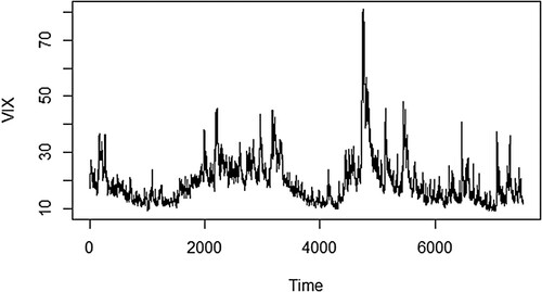
In this section, we take S&P 500 VIX as an example to investigate the performance of our proposed method. VIX is a real-time index also known as Fear Index derived from the price inputs of option. As a forward looking index, it represents the market's expectations for volatility over the coming 30 days. It is a measurement for investors to make investment decision by the level of market risk, fear or stress because there is a strong negative correlation between volatility and the stock market returns demonstrated by historical data. It is also useful for traders to price its derivatives by VIX values. Moreover, if it is extended to the price observations of the broader market level index, such as the S&P 500 index, we will get a peek into volatility of the larger market. Hence, for comparing the possible price moves and the risk easily, it is meaningful to find a standard quantitative measure for volatility. The data are collected from 2/1/1990 to 21/11/2019 and available from https://finance.yahoo.com/quote/%5EVIX/history?p=%5EVIX. The VIX series trajectory is shown in Figure 1. By the autocorrelation test, we find that the series is stationary and with long-memory.

Figure 1. The S$\mathrm{\&}$P 500 VIX series.

Our aim of this study is to verify the validity of our proposed ET method for constructing confidence region. When we use an ARFIMA(1, d,0) model with parameter $(\varphi ,d)$ to fit the data, the ET point estimates of parameters listed in Table 8 do not change the original characteristics of the data even the moment model may be misspecified and just-identified. However, the EL and ETEL estimates of $(\varphi ,d)$ violate the stationary and long memory properties of this series. This is consistent of the theory we stated in Section 2.3; ET method is more superior in the case of model misspecification than the EL and ETEL method. The data-driven AET-based confidence region is depicted in Figure 2.

Figure 2. 95% confidence region of the parameters for fitted ARFIMA(1,d,0) of the S&P 500 VIX series.

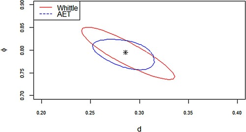
Table 8. Point estimates of the parameter vector $(\varphi ,d)$ by the three methods.

EL	ET	ETEL
(0.0815,0.7961)	(0.7952,0.2856)	(0.0812,0.7963)

4. Conclusion

In this paper, we propose ET method to infer the spectral parameters in stationary time series models. By comparing the coverage probabilities, we find that the adjusted technique also plays the best utility while enhancing computational efficiency and estimation accuracy for ET, which illustrates that the adjustment technique is useful and not limited to EL. Moreover, in view of point estimate, we highlight that the ET method outperforms EL and ETEL methods under the misspecified over-identified moment models. And the superiority of our proposed method is verified in numerical studies.

It is interesting to develop the other corrected ET to make the based coverage regions more accurate under the small sample size case. One possible way may be modifying the adjustment procedure. It can be carried out through adding two or more pseudo samples, which makes the solution of estimating equations exist and further improves the under-coverage. Another possible improvement may be realized by obtaining the estimating functions from other ways such as de-biased Whittle likelihood or tapered periodogram which make estimate of the parameter with a smaller bias. Another direction of our future study is extending the ET method in stationary time series model with time-varying variances, which is motivated by recent work of Han and Zhang (2021).

Disclosure statement

No potential conflict of interest was reported by the author(s).

Additional information

Funding

This work was supported by Natural Science Foundation of Shanghai (17ZR1409000), National Natural Science Foundation of China (11831008, 11971171) and the Open Research Fund of Key Laboratory of Advanced Theory and Application in Statistics and Data Science-MOE, ECNU.

Appendix

In this section, we give the brief proof of the main results. To simplify the notation in all of the proofs, we introduce some notes. Let $\lambda :={\lambda }_{\text{β}}$, ${\psi }_i:={\psi }_i\left\{I\right({\omega }_i),\text{β}\}$, $\overline{\psi }:=\frac{1}{n}\sum _i{\psi }_i$, ${\mathrm{\Psi }}_i:=\mathrm{\partial }{\psi }_i/\mathrm{\partial }\text{β}$, $\overline{\mathrm{\Psi }}:=\frac{1}{n}\sum _i{\mathrm{\Psi }}_i$, $V:=\frac{1}{n}\sum _i{\psi }_i{\psi }_i^{\tau }$, the equalities evaluate at point ${\text{β}}^{\ast }$ with superscript ${}^{\ast }$.

Proof of Theorem 2.1.

Note $Z_n=\underset{1\le i\le n}{max}\parallel {\psi }_i\parallel$, then $Z_n=o_p\left(n^{1/2}\right)$. In fact, $\begin{array}{rl}P(|Z_n/\sqrt{n}|\ge c)& =1-P(|Z_n{|}^2<c^{2}n)\\ & =1-\prod _{j=1}^{n}P(\Vert {\psi }_i{\Vert }^2<c^{2}n)\\ & =1-\prod _{j=1}^n(1-P(\parallel {\psi }_i{\parallel }^2\ge c^{2}n)).\end{array}$By dominated convergence theorem, we have $\underset{n\to \mathrm{\infty }}{lim}P(\Vert {\psi }_i{\Vert }^2\ge c^{2}n)=0$ when $E\parallel {\psi }_i{\parallel }^2<\mathrm{\infty }$ and $\overline{\psi }=O_p\left(n^{-1/2}\right)$. By the Theorem 3 of Newey and Smith (2004), we immediately have $\lambda =O_p\left(n^{-1/2}\right)$. Next we will show that $R\left({\text{β}}^{\ast }\right)$ converges to a chi-square distribution. Note ${\eta }_j=n{\hat{p}}_j-1$, then by Taylor expansion, $\begin{array}{rl}{\eta }_j& =\frac{n\exp \left({\lambda }^{\tau }{\psi }_j\right)-\sum _{k=1}^n\exp \left({\lambda }^{\tau }{\psi }_k\right)}{\sum _{k=1}^n\exp \left({\lambda }^{\tau }{\psi }_k\right)}\\ & ={\lambda }^{\tau }({\psi }_j-\overline{\psi })+o_p\left({\lambda }^2\right).\end{array}$Then, $\begin{array}{rl}R\left(\text{β}\right)& =4\sum _{j=1}^{n}n{\hat{p}}_j\log \left(n{\hat{p}}_j\right)\\ & =4\sum _{j=1}^n(({\eta }_j+1)\log (1+{\eta }_j))\\ & =4\sum _{j=1}^n({\eta }_j+\frac{{\eta }_j^2}{2}+o_p\left({\eta }_j^2\right))\\ & =2\sum _{j=1}^n({\eta }_j^2+o_p\left({\lambda }^2\right))\\ & ={\lambda }^{\tau }\sum _{j=1}^n({\psi }_j-\overline{\psi })({\psi }_j-\overline{\psi }{)}^{\tau }\lambda +o_p(1)\\ & ={\lambda }^{\tau }\left(\sum _{j=1}^n{\psi }_j{\psi }_j^{\tau }\right)\lambda +o_p\left(1\right),\end{array}$where λ satisfies Eq. (1(1) $\sum _{j=1}^n\exp ({\lambda }^{\tau }{\psi }_j\left\{I\right({\omega }_j),\text{β}\}){\psi }_j\left\{I\right({\omega }_j),\text{β}\}=0.$(1) ). By Taylor expansion of Eq. (1(1) $\sum _{j=1}^n\exp ({\lambda }^{\tau }{\psi }_j\left\{I\right({\omega }_j),\text{β}\}){\psi }_j\left\{I\right({\omega }_j),\text{β}\}=0.$(1) ), we have (A1) $\begin{array}{rl}\lambda & =-{\left(\frac{1}{n}\sum _{j=1}^n{\psi }_j{\psi }_j^{\tau }\right)}^{-1}\left(\frac{1}{n}\sum _{j=1}^n{\psi }_j\right)+o_p\left(n^{-1/2}\right)\\ & =-V^{-1}\overline{\psi }+o_p\left(n^{-1/2}\right).\end{array}$(A1) In fact, because Whittle estimate $\widehat{\text{β}}$ satisfies $\Vert \widehat{\text{β}}-{\text{β}}^{\ast }\Vert =O_p\left(n^{-1/2}\right)$, then $\begin{array}{rl}{\overline{\psi }}^{\ast }& =\overline{\mathrm{\Psi }}{|}_{\text{β}=\widehat{\text{β}}}({\text{β}}^{\ast }-\widehat{\text{β}})+o_p\left(n^{-1/2}\right)\mathrm{a}\mathrm{n}\mathrm{d}\\ V^{\ast }& =V{|}_{\text{β}=\widehat{\text{β}}}+O_p\left(n^{-1/2}\right).\end{array}$Substituting ${\overline{\psi }}^{\ast }$ and $V^{\ast }$ in λ, we have ${\lambda }^{\ast }=-V^{-1}{|}_{\text{β}=\widehat{\text{β}}}\overline{\mathrm{\Psi }}{|}_{\text{β}=\widehat{\text{β}}}({\text{β}}^{\ast }-\widehat{\text{β}})+o_p\left(n^{-1/2}\right).$Then substituting ${\lambda }^{\ast }$ and $V^{\ast }$ into $R\left({\text{β}}^{\ast }\right)$, by Lemma 6 of Nordman and Lahiri (2006), we have $R\left({\text{β}}^{\ast }\right)$ which converges to the chi-square distribution with degree k of freedom.

Proof of Theorem 2.2.

By the proof of Theorem 2.1 and Eq. (4(4) $\sum _{j=1}^{n+1}\exp ({\lambda }^{\tau }{\psi }_j\left\{I\right({\omega }_j),\text{β}\}){\psi }_j\left\{I\right({\omega }_j),\text{β}\}=0.$(4) ), we have $\begin{array}{rl}0& =\frac{1}{n}\sum _{j=1}^{n+1}\exp \left({\lambda }^{\tau }{\psi }_j\right){\psi }_j\\ & =\frac{1}{n}\sum _{j=1}^{n+1}(1+{\lambda }^{\tau }{\psi }_j+o\left({\lambda }^{\tau }{\psi }_j\right)){\psi }_j\\ & =\overline{\psi }(1-\frac{a}{n})+\frac{1}{n}\sum _{j=1}^{n+1}{\psi }_j{\psi }_j^{\tau }\lambda +o_p\left(n^{-1/2}\right)\\ & =\overline{\psi }+\frac{1}{n}\sum _{j=1}^n{\psi }_j{\psi }_j^{\tau }\lambda +o_p\left(n^{-1/2}\right),\end{array}$where $a=max\{1,\log n/2\}=o\left(n\right)$. Thus, we have $\lambda =-V^{-1}\overline{\psi }+o_p\left(n^{-1/2}\right).$ Similar to the proof of Theorem 2.1, because $(n+1){\hat{p}}_j^A-1={\eta }_j$, we expand $R(\text{β};a)$ as $\begin{array}{rl}R(\text{β};a)& =4(n+1)\sum _{j=1}^{n+1}{\hat{p}}_j^A\log \left(\right(n+1\left){\hat{p}}_j^A\right)\\ & =2\sum _{j=1}^{n+1}({\eta }_j^2+o_p\left({\lambda }^2\right))\\ & =2\sum _{j=1}^n({\eta }_j^2+o_p\left(1\right)).\end{array}$Then $R({\text{β}}^{\ast };a)⟶{\chi }_k^2$ in distribution.

For proving Theorem 2.3, we require the additional lemma stated as follows. By introducing the additional parameters, the construction of the equations is equivalent to that of the just-identified GMM procedure (Schennach, 2007).

Lemma A.1

Let $\hat{\theta }=(\hat{\kappa },\hat{\lambda },\widehat{\text{β}})$ be the ET estimator of $\theta =(\kappa ,\lambda ,\text{β}),$ where $\kappa =1/n\sum _i{\kappa }_i$ with ${\kappa }_i=\exp \left({\lambda }^{\tau }{\psi }_i\right)$. Then, $\hat{\theta }$ is the solution to $\frac{1}{n}\sum _i{\varpi }_i=0,$ where ${\varpi }_i={\varpi }_i\left\{I\right({\omega }_i),\theta \}=({\kappa }_i-\kappa ,{\kappa }_i{\psi }_i^{\tau },{\kappa }_i({\mathrm{\Psi }}_i^{\tau }\lambda {)}^{\tau }{)}^{\tau }.$

Proof of Lemma A.1.

It is obvious that $\frac{1}{n}\sum _i({\kappa }_i-\kappa )=0$ holds by its definition and λ satisfies the equation $\frac{1}{n}\sum _i{\kappa }_i{\psi }_i=0$. Because $\widehat{\text{β}}$ minimizes the likelihood ratio $l\left(\text{β}\right)$, then the first-order condition for β can be expressed by equation $\mathrm{\partial }l\left(\text{β}\right)/\mathrm{\partial }{\text{β}}^{\tau }=0$, that is, $\frac{1}{n}\sum _i{\kappa }_i{\mathrm{\Psi }}_i^{\tau }\lambda =0$. Then we complete the proof.

Proof of Theorem 2.3.

In this proof, all the elements with superscript ${}^{\ast }$ mean the values corresponding to pseudo-true value ${\text{β}}^{\ast }$. The proof of Theorem 2.3(i) is completely similar to the proof of Theorem 10 (Schennach, 2007), hence is omitted. For proving 2.3(ii), we restrict our attention to the just-identified equations of Lemma A.1. Applying Theorem 3.4 of Newey and McFadden (1994), we only need to show that

1. $E[\underset{\theta \in \mathrm{\Theta }}{sup}\Vert \mathrm{\partial }{\varpi }_i/\mathrm{\partial }\theta \Vert ]<\mathrm{\infty }$ for some neighbourhood Θ of ${\theta }^{\ast }$.

2. $E\left[{\varpi }_i\right\{I\left({\omega }_i\right),{\theta }^{\ast }\left\}{\varpi }_i\right\{I\left({\omega }_i\right),{\theta }^{\ast }{\}}^{\tau }]$ exists.

Since then ψ, Ψ and V represent the elements of ${\psi }_i$, ${\mathrm{\Psi }}_i$ and $V_{jl}\left\{I\right({\omega }_i),\text{β}\}$, respectively. All of the components of the matrix $\mathrm{\partial }{\varpi }_i/\mathrm{\partial }\theta$ take the form of $\alpha \exp \left(n_{\kappa }{\lambda }^{\tau }{\psi }_i\right){\psi }^{n_{\psi }}{\mathrm{\Psi }}^{n_{\mathrm{\Psi }}}{V}^{n_V}$ for $n_{\psi }+n_{\mathrm{\Psi }}+n_V\le 2$ and $n_{\kappa }=0,1$, where α represents the products of elements of θ which are bounded for $\theta \in \mathrm{\Theta }$. Then by Assumption 2.1, we have $\begin{array}{rl}& E[\underset{\theta \in \mathrm{\Theta }}{sup}\exp (n_{\kappa }{\lambda }^{\tau }{\psi }_i\left)|\psi {|}^{n_{\psi }}|\mathrm{\Psi }{|}^{n_{\mathrm{\Psi }}}|V{|}^{n_V}\right]\\ & \le E[\underset{\theta \in \mathrm{\Theta }}{sup}\exp (n_{\kappa }{\lambda }^{\tau }{\psi }_i\left)\right(h\left\{I\right({\omega }_i\left)\right\}{)}^{k_2}]\\ & =E[\underset{\text{β}\in {\mathcal{B}}^{\ast }}{sup}\underset{\lambda \in \mathrm{\Lambda }\left(\text{β}\right)}{sup}\exp (n_{\kappa }{\lambda }^{\tau }{\psi }_i\left)\right(h\left\{I\right({\omega }_i\left)\right\}{)}^{k_2}]<\mathrm{\infty }.\end{array}$

This is because $\exp \left(n_{\kappa }{\lambda }^{\tau }{\psi }_i\right)|\psi {|}^{n_{\psi }}|\mathrm{\Psi }{|}^{n_{\mathrm{\Psi }}}|V{|}^{n_V}\le \exp \left(n_{\kappa }{\lambda }^{\tau }{\psi }_i\right)|h\left\{I\right({\omega }_i\left)\right\}{|}^{n_{\psi }+n_{\mathrm{\Psi }}+n_V}$. Similarly, the elements of matrix ${\varpi }_i\left\{I\right({\omega }_i),\theta \}{\varpi }_i\left\{I\right({\omega }_i),\theta {\}}^{\tau }$ take the form of $\alpha \exp \left(n_{\kappa }{\lambda }^{\tau }{\psi }_i\right)|\psi {|}^{n_{\psi }}|\mathrm{\Psi }{|}^{n_{\mathrm{\Psi }}}$ with $0\le n_{\psi }+n_{\mathrm{\Psi }}\le 2$ and $n_{\kappa }=0,1,2$. Hence, the similar procedure implies (II).

References

- Brillinger, D. R. (1981). Time series: Data analysis and theory. Holden-Day.
- Caner, M. (2010). Exponential tilting with weak instruments: Estimation and testing. Oxford Bulletin of Economics and Statistics, 72(3), 307–325. https://doi.org/10.1111/obes.2010.72.issue-3
- Chan, N. H., & Liu, L. (2010). Bartlett correctability of empirical likelihood in time series. Journal of the Japan Statistical Society, 40(2), 221–238. https://doi.org/10.14490/jjss.40.221
- Chen, J. H., Variyath, A. M., & Abraham, B. (2008). Adjusted empirical likelihood and its properties. Journal of Computational and Graphical Statistics, 17(2), 426–443. https://doi.org/10.1198/106186008X321068
- DiCiccio, T., Hall, P., & Romano, J. (1991). Empirical likelihood is Bartlett correctable. The Annals of Statistics, 19(2), 1053–1061. https://doi.org/10.1214/aos/1176348137
- Granger, C. W. J., & Joyeux, R. (1980). An introduction to long-memory time series models and fractional differencing. Journal of Time Series Analysis, 1(1), 15–29. https://doi.org/10.1111/j.1467-9892.1980.tb00297.x
- Han, Y., & Zhang, C. M. (2021). Empirical likelihood inference in autoregressive models with time-varying variances. Statistical Theory and Related Fields. https://doi.org/10.1080/24754269.2021.1913977
- Hosking, J. R. M. (1981). Fractional differencing. Biometrika, 68(1), 165–176. https://doi.org/10.1093/biomet/68.1.165
- Imbens, G. W. (2002). Generalized method of moments and empirical likelihood. Journal of Business and Economic Statistics, 20(4), 493–506. https://doi.org/10.1198/073500102288618630
- Imbens, G. W., Spady, R. H., & Johnson, P. (1998). Information-theoretic approaches to inference in moment condition models. Econometrica, 66(2), 333–357. https://doi.org/10.2307/2998561
- Jing, B. Y., & Andrew, T. A. (1996). Exponential empirical likelihood is not Bartlett correctable. The Annals of Statistics, 24(1), 365–369. https://doi.org/10.1214/aos/1033066214
- Kitamura, Y. (1997). Empirical likelihood methods with weakly dependent processes. The Annals of Statistics, 25(5), 2084–2102. https://doi.org/10.1214/aos/1069362388
- Kitamura, Y. (2000). Comparing misspecified dynamic econometric models using nonparametric likelihood. Department of Economics, University of Wisconsin.
- Kitamura, Y., & Stutzer, M. (1997). An information-theoretic alternative to generalized method of moments estimation. Econometrica, 65(4), 861–874. https://doi.org/10.2307/2171942
- Liu, Y. K., & Chen, J. H. (2010). Adjusted empirical likelihood with high-order precision. The Annals of Statistics, 38(3), 1341–1362. https://doi.org/10.1214/09-aos750
- Monti, A. C. (1997). Empirical likelihood confidence regions in time series models. Biometrika, 84(2), 395–405. https://doi.org/10.1093/biomet/84.2.395
- Newey, W. K., & McFadden, D. (1994). Large sample estimation and hypothesis testing (4th ed.). North-Holland, pp. 2111–2245.
- Newey, W. K., & Smith, R. J. (2004). Higher order properties of GMM and generalized empirical likelihood estimators. Econometrica, 72(1), 219–255. https://doi.org/10.1111/ecta.2004.72.issue-1
- Nordman, D. J., & Lahiri, S. N. (2006). A frequency domain empirical likelihood for short- and long-range dependence. The Annals of Statistics, 34(6), 3019–3050. https://doi.org/10.1214/009053606000000902
- Nordman, D. J., & Lahiri, S. N. (2014). A review of empirical likelihood methods for time series. Journal of Statistical Planning and Inference, 155, 1–18. https://doi.org/10.1016/j.jspi.2013.10.001
- Owen, A. B. (1988). Empirical likelihood ratio confidence intervals for a single functional. Biometrika, 75(2), 237–249. https://doi.org/10.1093/biomet/75.2.237
- Owen, A. B. (1990). Empirical likelihood ratio confidence regions. The Annals of Statistics, 18(1), 90–120. https://doi.org/10.1214/aos/1176347494
- Owen, A. B. (2001). Empirical likelihood. Chapman & Hall.
- R. D. Piyadi Gamage, Ning, W., & Gupta, A. K. (2017a). Adjusted empirical likelihood for long-memory time series models. Journal of Statistical Theory and Practice, 11(1), 220–233. https://doi.org/10.1080/15598608.2016.1271373
- Piyadi Gamage, R. D., Ning, W., & Gupta, A. K. (2017b). Adjusted empirical likelihood for time series models. Sankhya series B, 79(2), 336–360. https://doi.org/10.1007/s13571-017-0137-y
- Schennach, S. M. (2005). Bayesian exponentially tilted empirical likelihood. Biometrika, 92(1), 31–46. https://doi.org/10.1093/biomet/92.1.31
- Schennach, S. M. (2007). Point estimation with exponentially tilted empirical likelihood. The Annals of Statistics, 35(2), 634–672. https://doi.org/10.1214/009053606000001208
- Tang, N. S., Yan, X. D., & Zhao, P. Y. (2018). Exponentially tilted likelihood inference on growing dimensional unconditional moment models. Journal of Econometrics, 202(1), 57–74. https://doi.org/10.1016/j.jeconom.2017.08.018
- Whittle, P. (1953). Estimation and information in stationary time series. Arkiv för Matematik, 2(5), 423–434. https://doi.org/10.1007/BF02590998
- Yau, C. Y. (2012). Empirical likelihood in long-memory time series models. Journal of Time Series Analysis, 33(2), 269–275. https://doi.org/10.1111/jtsa.2012.33.issue-2
- Zhu, H., Zhou, H., Chen, J., Li, Y., Lieberman, J., & Styner, M. (2009). Adjusted exponentially tilted likelihood with applications to brain morphology. Biometrics, 65(3), 919–927. https://doi.org/10.1111/j.1541-0420.2008.01124.x