High-dimensional proportionality test of two covariance matrices and its application to gene expression data

Abstract

With the development of modern science and technology, more and more high-dimensional data appear in the application fields. Since the high dimension can potentially increase the complexity of the covariance structure, comparing the covariance matrices among populations is strongly motivated in high-dimensional data analysis. In this article, we consider the proportionality test of two high-dimensional covariance matrices, where the data dimension is potentially much larger than the sample sizes, or even larger than the squares of the sample sizes. We devise a novel high-dimensional spatial rank test that has much-improved power than many existing popular tests, especially for the data generated from some heavy-tailed distributions. The asymptotic normality of the proposed test statistics is established under the family of elliptically symmetric distributions, which is a more general distribution family than the normal distribution family, including numerous commonly used heavy-tailed distributions. Extensive numerical experiments demonstrate the superiority of the proposed test in terms of both empirical size and power. Then, a real data analysis demonstrates the practicability of the proposed test for high-dimensional gene expression data.

Keywords:

• Covariance matrices
• elliptically symmetric distributions
• high dimension test
• proportionality
• spatial rank

1. Introduction

High-dimensional data are nowadays more and more common in bioinformatics, material science, astronomy and other application fields, as data collection technology rapidly evolves (Bühlmann & van de Geer, 2011). However, due to limited resources available to replicate observations, the sample sizes are usually much smaller than the dimension, which makes most traditional statistical approaches no longer appropriate. Under such an embarrassing background, scientists in many application fields urgently need powerful approaches to gather the greatest scientific insight from data. Testing equality of the distributions of two populations is a crucial problem in high-dimensional statistics, which is extremely complex and far more challenging than that for fixed-dimensional data. Due to this extreme complexity, it is usually replaced by a simpler problem, i.e. testing equality of some numerical characteristics, such as means and covariances, of the two populations, which is very useful but much easier to implement.

There is already a large number of literature on detecting the difference between the means of two high-dimensional populations, such as Bai and Saranadasa (1996), Chen and Qinm (2010), and Feng et al. (2016), to name just a few. In contrast, there are much fewer studies on high-dimensional covariance matrix test of two high-dimensional populations. Hence, in this article, we focus on comparing the covariance matrices among two populations, which is strongly motivated for high-dimensional data, as high data dimensions can potentially increase the complexity of the covariance structure (Li & Chen, 2012). In particular, we consider the testing problem of the proportionality of two high-dimensional covariance matrices, which investigates the simplest heteroscedasticity of the population covariance matrices (Xu et al., 2014). It is often a preparation procedure before the case–control analysis of genomic data. Let $\mathit{X}$ and $\mathit{Y}$ be two p-dimensional populations with the mean vectors ${\mathit{\mu }}_1$, ${\mathit{\mu }}_2$ and the covariance matrices ${\mathbf{\Sigma }}_1$, ${\mathbf{\Sigma }}_2$, respectively. The proportionality test of two population covariance matrices is formulated as follows: (1) $H_0:{\mathbf{\Sigma }}_1=c{\mathbf{\Sigma }}_2\mathrm{v}\mathrm{e}\mathrm{r}\mathrm{s}\mathrm{u}\mathrm{s}{H}_1:{\mathbf{\Sigma }}_1\ne c{\mathbf{\Sigma }}_2,$(1) where c is an unknown scalar.

The proportionality testing problem in (1(1) $H_0:{\mathbf{\Sigma }}_1=c{\mathbf{\Sigma }}_2\mathrm{v}\mathrm{e}\mathrm{r}\mathrm{s}\mathrm{u}\mathrm{s}{H}_1:{\mathbf{\Sigma }}_1\ne c{\mathbf{\Sigma }}_2,$(1) ) has been widely studied in various areas, such as in discriminant analysis and principal component analysis (Flury & Riedwyl, 1988; Schott, 1991), and there is a lot of early literature on its methodological researches, such as Eriksen (1987), Federer (1951), Flury (1986), Kim (1971), Rao (1983), and Schott (1999). For example, the most traditional test statistic is $\begin{array}{rl}& (n_1+n_2)\sum _{j=1}^p\log \left({\hat{\lambda }}_j\right)-n_1\log \left(|{\hat{\mathbf{\Sigma }}}_1|\right)\\ & +n_2(p\log (\hat{c}-\log \left(|{\hat{\mathbf{\Sigma }}}_2|\right)\left)\right)\stackrel{d}{\to }{\chi }_{(p^2+p-2)/2}^2,\end{array}$where $({\hat{\lambda }}_j,\hat{c})$ are obtained by an iterative algorithm proposed in Flury (1986) and ${\hat{\mathbf{\Sigma }}}_1,{\hat{\mathbf{\Sigma }}}_2$ are the corresponding sample covariance matrices, respectively. These researches are constructed based on the classical limit theorems, assuming that the sample sizes tend to infinity and the dimension is fixed, hence have difficulties to analyse the high-dimensional data, where the dimension is much larger than the sample sizes. To alleviate such difficulties, Xu et al. (2014) proposed to use a pseudo-likelihood ratio test by extending the traditional likelihood ratio test with the statistic $p\log \left(p^{-1}\mathrm{t}\mathrm{r}\right({\hat{\mathbf{\Sigma }}}_1{\hat{\mathbf{\Sigma }}}_2^{-1}\left)\right)-\log |{\hat{\mathbf{\Sigma }}}_1{\hat{\mathbf{\Sigma }}}_2^{-1}|,$ which allows the dimension to increase proportionally with each sample size; furthermore, Liu et al. (2014) proposed an improved method, which allows the dimension to be larger than one of the sample sizes. In addition, for the special case of $c\equiv 1$ in (1(1) $H_0:{\mathbf{\Sigma }}_1=c{\mathbf{\Sigma }}_2\mathrm{v}\mathrm{e}\mathrm{r}\mathrm{s}\mathrm{u}\mathrm{s}{H}_1:{\mathbf{\Sigma }}_1\ne c{\mathbf{\Sigma }}_2,$(1) ), Li and Chen (2012) proposed a test statistic $T_{LC}=A_{n_1}+A_{n_2}-2C_{n_1,n_2},$where $\begin{array}{rl}{A}_{n_i}& =\frac{1}{n_i(n_i-1)}\sum _{k\ne l}({\mathit{X}}_{ik}^{\mathrm{\top }}{\mathit{X}}_{il}{)}^2\\ & -\frac{2}{n_i(n_i-1)(n_i-2)}\sum _{j,k,l\mathrm{n}\mathrm{o}\mathrm{t}\mathrm{e}\mathrm{q}\mathrm{u}\mathrm{a}\mathrm{l}}{\mathit{X}}_{ik}^{\mathrm{\top }}{\mathit{X}}_{ij}{\mathit{X}}_{ij}^{\mathrm{\top }}{\mathit{X}}_{il}\\ & +\frac{1}{n_i(n_i-1)(n_i-2)(n_i-3)}\\ & \sum _{j,k,l,t\mathrm{n}\mathrm{o}\mathrm{t}\mathrm{e}\mathrm{q}\mathrm{u}\mathrm{a}\mathrm{l}}{\mathit{X}}_{ik}^{\mathrm{\top }}{\mathit{X}}_{ij}{\mathit{X}}_{it}^{\mathrm{\top }}{\mathit{X}}_{il},\\ C_{n_1,n_2}& =\frac{1}{n_1{n}_2}\sum _{k=1}^{n_1}\sum _{l=1}^{n_2}({\mathit{X}}_{1k}^{\mathrm{\top }}{\mathit{X}}_{2l}{)}^2\\ & -\frac{1}{n_1{n}_2(n_1-1)}\sum _{k\ne l}^{n_1}\sum _{j=1}^{n_2}{\mathit{X}}_{1k}^{\mathrm{\top }}{\mathit{X}}_{2j}{\mathit{X}}_{2j}^{\mathrm{\top }}{\mathit{X}}_{1l}\\ & -\frac{1}{n_1{n}_2(n_2-1)}\sum _{k\ne l}^{n_2}\sum _{j=1}^{n_1}{\mathit{X}}_{2k}^{\mathrm{\top }}{\mathit{X}}_{1j}{\mathit{X}}_{1j}^{\mathrm{\top }}{\mathit{X}}_{2l}\\ & +\frac{1}{n_1{n}_2(n_1-1)(n_2-1)}\\ & \times \sum _{k\ne t}^{n_1}\sum _{j\ne l}^{n_2}{\mathit{X}}_{1k}^{\mathrm{\top }}{\mathit{X}}_{2j}{\mathit{X}}_{1t}^{\mathrm{\top }}{\mathit{X}}_{2l}.\end{array}$As mentioned in Li and Chen (2012), $T_{LC}$ is an unbiased estimation of $\mathrm{t}\mathrm{r}\left\{\right({\mathbf{\Sigma }}_1-{\mathbf{\Sigma }}_2{)}^2\}$. Despite some progress, there are also drawbacks: first, these methods may have extremely poor performance for heavy-tailed distributions; second, the sample covariance matrices, which need to be inverted in the construction of the test statistic, are singular when the dimension is larger than both of the sample sizes.

To overcome these two drawbacks, more attention has been paid to nonparametric testing methods based on the multivariate sign or rank. Just recently, for testing the proportionality of two high-dimensional covariance matrices, Cheng et al. (2018) proposed to use a test procedure based on the multivariate sign and demonstrated its good performance in high-dimensional data analysis, especially for the heavy-tailed distributions. Recall that for fixed-dimensional data, the multivariate sign and rank are widely used to construct robust tests (Oja, 2010). However, most of these tests cannot be effective for high-dimensional data. Therefore, many researches extend the traditional multivariate sign- or rank-based testing methods to the high-dimension data, such as Feng and Sun (2016) and Wang et al. (2015) for one-sample problems; Feng et al. (2016) for two-sample problems; Feng and Liu (2017) and Zou et al. (2014) for sphericity testing problems. These researches clearly demonstrate the advantages of the high-dimensional multivariate sign- or rank-based methods in high-dimensional and heavy-tailed cases.

Unfortunately, due to the bias caused by estimating the location parameters, the test procedure based on the multivariate sign can only allow the dimension to be the squares of the sample sizes at most (Cheng et al., 2018), which makes the test procedure too restrictive for various practical applications, hence greatly affects the validity of the test procedure. For example, in genomic data analysis, genomic data typically carry thousands of dimensions for measurements on the genome, where the dimension can be much larger than the squares of the sample sizes. Therefore, it is very urgent to develop a new method to deal with the proportionality testing problem in (1(1) $H_0:{\mathbf{\Sigma }}_1=c{\mathbf{\Sigma }}_2\mathrm{v}\mathrm{e}\mathrm{r}\mathrm{s}\mathrm{u}\mathrm{s}{H}_1:{\mathbf{\Sigma }}_1\ne c{\mathbf{\Sigma }}_2,$(1) ) for the high-dimensional data, where the dimension is much higher than the squares of the sample sizes. This is the motivation and intention of this article.

The rest of the article is organized as follows. In Section 2, we introduce the proposed high-dimensional spatial rank test and establish its asymptotic normality under the elliptically symmetric populations. Then, we demonstrate the numerical performance of the proposed test in Sections 3, followed by a real data analysis in Section 4. Finally, we conclude this article in Section 5 and relegate the technical proofs to Appendix.

2. Method

2.1. The proposed test

A p-dimensional random vector $\mathit{Z}$ is said to follow an elliptically symmetric distribution, denoted by ${\mathcal{E}}_p(\mathit{\mu },\mathbf{\Lambda },F_{\xi })$, if it has the following stochastic representation: $\mathit{Z}=\mathit{\mu }+\xi \mathbf{A}\mathbf{U},$where $\mathit{\mu }$ is the p-dimensional mean vector, ξ is a non-negative random variable, $F_{\xi }$ is the cumulative distribution function of ξ, $\mathbf{U}$ is independent of ξ and is uniformly distributed on the unit sphere ${\mathcal{R}}^p$ and $\mathbf{A}$ is a deterministic $p\times p$-dimensional matrix satisfying $\mathbf{A}{\mathbf{A}}^{\mathrm{T}}=\mathbf{\Lambda }$ with $\mathrm{t}\mathrm{r}\left(\mathbf{\Lambda }\right)=1$. It is known that the covariance matrix $\mathbf{\Sigma }$ and shape matrix $\mathbf{\Lambda }$ of the elliptical symmetric population $\mathit{Z}$ will satisfy the equation $\mathbf{\Sigma }=p^{-1}E\left({\xi }^2\right)\mathbf{\Lambda }$.

Let ${\mathit{X}}_1,\dots ,{\mathit{X}}_{n_1}$ and ${\mathit{Y}}_1,\dots ,{\mathit{Y}}_{n_2}$ denote the samples of two p-dimensional random vectors $\mathit{X}$ and $\mathit{Y}$, which are generated from the two independent elliptically symmetric populations ${\mathcal{E}}_p({\mathit{\mu }}_1,{\mathbf{\Lambda }}_1,F_{{\xi }_1})$ and ${\mathcal{E}}_p({\mathit{\mu }}_2,{\mathbf{\Lambda }}_2,F_{{\xi }_2})$, respectively. From Section 3.1 in Magyar and Tyler (2014), it is known that ${\mathbf{\Sigma }}_i$ and ${\mathrm{\S }}_i$ have the same eigenvectors for each $i\in \{1,2\}$ under the assumption of elliptically symmetric distribution. Also, from Equation 3.9 in Magyar and Tyler (2014), it is known that when the eigenvalues of the covariance matrices ${\mathbf{\Sigma }}_1$ and ${\mathbf{\Sigma }}_2$ are proportional, the spatial sign covariance matrices ${\mathrm{\S }}_1$ and ${\mathrm{\S }}_2$ have the same eigenvalues. Theorem 1 in Cheng et al. (2018) showed that when ${\mathrm{\S }}_1$ and ${\mathrm{\S }}_2$ have the same eigenvalues, the eigenvalues of ${\mathbf{\Sigma }}_1$ and ${\mathbf{\Sigma }}_2$ are proportional. Hence, the hypotheses in (1(1) $H_0:{\mathbf{\Sigma }}_1=c{\mathbf{\Sigma }}_2\mathrm{v}\mathrm{e}\mathrm{r}\mathrm{s}\mathrm{u}\mathrm{s}{H}_1:{\mathbf{\Sigma }}_1\ne c{\mathbf{\Sigma }}_2,$(1) ) are equivalent to the following hypotheses: (2) $H_0:{\mathrm{\S }}_1={\mathrm{\S }}_2\mathrm{v}\mathrm{e}\mathrm{r}\mathrm{s}\mathrm{u}\mathrm{s}{H}_1:{\mathrm{\S }}_1\ne {\mathrm{\S }}_2,$(2) where ${\mathrm{\S }}_1=\mathbb{E}\left\{U\right(\mathit{X}-{\mathit{\mu }}_1\left)U\right(\mathit{X}-{\mathit{\mu }}_1{)}^{\mathrm{T}}\}$, ${\mathrm{\S }}_2=\mathbb{E}\left\{U\right(\mathit{Y}-{\mathit{\mu }}_2\left)U\right(\mathit{Y}-{\mathit{\mu }}_2{)}^{\mathrm{T}}\}$ are the spatial sign covariance matrices of $\mathit{X}$, $\mathit{Y}$, respectively, and $U\left(\mathbf{z}\right)=\frac{\mathbf{z}}{\Vert \mathbf{z}\Vert }I(\mathbf{z}\ne \mathbf{0})$ for each $\mathbf{z}\in {\mathcal{R}}^p$ is the spatial sign function with $\Vert \cdot \Vert$ denoting the $L_2$-norm and $I(\cdot )$ denoting the indicator function. On this ground, Cheng et al. (2018) suggested to use a test statistics based on the square Frobenius norm of ${\mathrm{\S }}_1-{\mathrm{\S }}_2$, i.e. $\mathrm{t}\mathrm{r}\left\{\right({\mathrm{\S }}_1-{\mathrm{\S }}_2{)}^2\}$.

The proposed spatial rank test in this article is also based on the square Frobenius norm of ${\mathrm{\S }}_1-{\mathrm{\S }}_2$, which is a high-dimensional extension of Kendall's tau test for the hypotheses in (2(2) $H_0:{\mathrm{\S }}_1={\mathrm{\S }}_2\mathrm{v}\mathrm{e}\mathrm{r}\mathrm{s}\mathrm{u}\mathrm{s}{H}_1:{\mathrm{\S }}_1\ne {\mathrm{\S }}_2,$(2) ) (Oja, 2010). Specifically, the test statistic is (3) $\begin{array}{rl}{T}_{\mathrm{H}\mathrm{T}}& =\frac{p}{n_1(n_1-1)(n_1-2)(n_1-3)}\\ & \times \sum ^{\ast }\left\{U\right({\mathit{X}}_i-{\mathit{X}}_j{)}^{\mathrm{T}}U({\mathit{X}}_k-{\mathit{X}}_l){\}}^2\\ & +\frac{p}{n_2(n_2-1)(n_2-2)(n_2-3)}\\ & \times \sum ^{\ast }\left\{U\right({\mathit{Y}}_i-{\mathit{Y}}_j{)}^{\mathrm{T}}U({\mathit{Y}}_k-{\mathit{Y}}_l){\}}^2\\ & -\frac{2p}{n_1(n_1-1)n_2(n_2-1)}\\ & \times \sum _{i=1}^{n_1}\sum _{j\ne i}^{n_1}\sum _{k=1}^{n_2}\sum _{l\ne k}^{n_2}\left\{U\right({\mathit{X}}_i-{\mathit{X}}_j{)}^{\mathrm{T}}U({\mathit{Y}}_k-{\mathit{Y}}_l){\}}^2,\end{array}$(3) where $\sum ^{\ast }$ denotes summation over distinct indexes $\{i,j,k,l\}\subseteq \{1,\dots ,n_1\}$ or $\{1,\dots ,n_2\}$. Note that recently many developed versions of Kendall's tau test are frequently used on many related issues (Barber & Kolar, 2018; Cai & Zhang, 2016; Han et al., 2017; Leung & Drton, 2018).

In deriving the asymptotic properties of $T_{\mathrm{H}\mathrm{T}}$, we impose the following two conditions used in Cheng et al. (2018):

1. $n_1/(n_1+n_2)\to \kappa \in (0,1)$ as $min\{n_1,n_2\}\to \mathrm{\infty }$;

2. $\mathrm{t}\mathrm{r}\left({\mathbf{\Lambda }}_i{\mathbf{\Lambda }}_j{\mathbf{\Lambda }}_k{\mathbf{\Lambda }}_l\right)=o\left\{\mathrm{t}\mathrm{r}\right({\mathbf{\Lambda }}_i{\mathbf{\Lambda }}_j\left)\mathrm{t}\mathrm{r}\right({\mathbf{\Lambda }}_k{\mathbf{\Lambda }}_l\left)\right\}$ for $i,j,k,l\in \{1,2\}$.

Note that: (1) Condition (C1) is a commonly used condition in high-dimensional two sample testing problems; (2) Condition (C2) is similar to Condition (A2) in Li and Chen (2012); (3) If all the eigenvalues of ${\mathbf{\Sigma }}_1$ and ${\mathbf{\Sigma }}_2$ are bounded, Condition (C2) holds.

Remark 2.1

Note that the above Conditions (C1) and (C2) do not contain any restriction on p and $n_1$, $n_2$, since such restriction is not needed to control the following terms: $\begin{array}{rl}& \sum _{i,j,k,l}\left\{U\right({\mathit{X}}_i-{\mathit{X}}_j{)}^{\mathrm{T}}U({\mathit{X}}_k-{\mathit{X}}_l){\}}^2\\ & -\sum ^{\ast }\left\{U\right({\mathit{X}}_i-{\mathit{X}}_j{)}^{\mathrm{T}}U({\mathit{X}}_k-{\mathit{X}}_l){\}}^2,\\ & \sum _{i,j,k,l}\left\{U\right({\mathit{Y}}_i-{\mathit{Y}}_j{)}^{\mathrm{T}}U({\mathit{Y}}_k-{\mathit{Y}}_l){\}}^2\\ & -\sum ^{\ast }\left\{U\right({\mathit{Y}}_i-{\mathit{Y}}_j{)}^{\mathrm{T}}U({\mathit{Y}}_k-{\mathit{Y}}_l){\}}^2,\\ & \sum _{i=1}^{n_1}\sum _{j=1}^{n_1}\sum _{k=1}^{n_2}\sum _{l=1}^{n_2}\left\{U\right({\mathit{X}}_i-{\mathit{X}}_j{)}^{\mathrm{T}}U({\mathit{Y}}_k-{\mathit{Y}}_l){\}}^2\\ & -\sum _{i=1}^{n_1}\sum _{j\ne i}^{n_1}\sum _{k=1}^{n_2}\sum _{l\ne k}^{n_2}\left\{U\right({\mathit{X}}_i-{\mathit{X}}_j{)}^{\mathrm{T}}U({\mathit{Y}}_k-{\mathit{Y}}_l){\}}^2,\end{array}$which have been removed from $T_{\mathrm{H}\mathrm{T}}$. That is to say, we remove all the items that include at least one pair of identical vectors, such as $\left\{U\right({\mathit{X}}_i-{\mathit{X}}_j{)}^{\mathrm{T}}U({\mathit{X}}_i-{\mathit{X}}_j){\}}^2$, $\left\{U\right({\mathit{X}}_i-{\mathit{X}}_j{)}^{\mathrm{T}}U({\mathit{X}}_i-{\mathit{X}}_l){\}}^2$ and so on. Such type of strategy was previously used in Chen and Qinm (2010). By removing the terms $\sum _i{\mathit{X}}_i^{\mathrm{T}}{\mathit{X}}_i$ and $\sum _k{\mathit{Y}}_k^{\mathrm{T}}{\mathit{Y}}_k$ from the test statistic proposed by Chen and Qinm (2010), no restriction on p, $n_1$ and $n_2$ is needed.

Under the above two conditions, the limiting null distribution of $T_{\mathrm{H}\mathrm{T}}$ is given in the following theorem.

Theorem 2.1

Under Conditions (C1), (C2) and $H_0$, as $n_1$, $n_2$, $p\to \mathrm{\infty }$, ${\sigma }_{0,n}^{-1}{T}_{\mathrm{H}\mathrm{T}}\stackrel{d}{\to }N(0,1),$where ${\sigma }_{0,n}^2=4(n_1^{-1}+n_2^{-1}{)}^2(p+2{)}^{-2}{\mathrm{t}\mathrm{r}}^2\left({\mathbf{\Lambda }}^2\right)$ with $\mathbf{\Lambda }={\mathbf{\Lambda }}_1={\mathbf{\Lambda }}_2$.

Moreover, we obtain the limiting distribution of $T_{\mathrm{H}\mathrm{T}}$ under $H_1$.

Theorem 2.2

Under Conditions (C1), (C2) and $H_1$, as $n_1$, $n_2$, $p\to \mathrm{\infty }$, ${\sigma }_n^{-1}[T_{\mathrm{H}\mathrm{T}}-p\mathrm{t}\mathrm{r}\{({\mathrm{\S }}_1-{\mathrm{\S }}_2{)}^2\}]\stackrel{d}{\to }N(0,1),$where $\begin{array}{rl}{\sigma }_n^2& =\frac{4}{n_1(n_1-1)}\frac{{\mathrm{t}\mathrm{r}}^2\left({\mathbf{\Lambda }}_1^2\right)}{(p+2{)}^2}+\frac{8}{n_1}\frac{p\mathrm{t}\mathrm{r}\left({\mathbf{\Lambda }}_1^4\right)-{\mathrm{t}\mathrm{r}}^2\left({\mathbf{\Lambda }}_1^2\right)}{p^2(p+2)}\\ & \times \frac{4}{n_2(n_2-1)}\frac{{\mathrm{t}\mathrm{r}}^2\left({\mathbf{\Lambda }}_2^2\right)}{(p+2{)}^2}+\frac{8}{n_2}\frac{p\mathrm{t}\mathrm{r}\left({\mathbf{\Lambda }}_2^4\right)-{\mathrm{t}\mathrm{r}}^2\left({\mathbf{\Lambda }}_2^2\right)}{p^2(p+2)}\\ & +\frac{8}{n_1{n}_2}\frac{{\mathrm{t}\mathrm{r}}^2\left({\mathbf{\Lambda }}_1{\mathbf{\Lambda }}_2\right)}{(p+2{)}^2}+(\frac{8}{n_1}+\frac{8}{n_2})\\ & \times \frac{p\mathrm{t}\mathrm{r}({\mathbf{\Lambda }}_1{\mathbf{\Lambda }}_2{)}^2-{\mathrm{t}\mathrm{r}}^2({\mathbf{\Lambda }}_1{\mathbf{\Lambda }}_2)}{p^2(p+2)}\\ & -\frac{16}{n_1}\frac{p\mathrm{t}\mathrm{r}\left({\mathbf{\Lambda }}_1^3{\mathbf{\Lambda }}_2\right)-\mathrm{t}\mathrm{r}\left({\mathbf{\Lambda }}_1{\mathbf{\Lambda }}_2\right)\mathrm{t}\mathrm{r}\left({\mathbf{\Lambda }}_1^2\right)}{p^2(p+2)}\\ & -\frac{16}{n_2}\frac{p\mathrm{t}\mathrm{r}\left({\mathbf{\Lambda }}_2^3{\mathbf{\Lambda }}_1\right)-\mathrm{t}\mathrm{r}\left({\mathbf{\Lambda }}_1{\mathbf{\Lambda }}_2\right)\mathrm{t}\mathrm{r}\left({\mathbf{\Lambda }}_2^2\right)}{p^2(p+2)}.\end{array}$

Due to the fact that $p\mathrm{t}\mathrm{r}\left({\mathrm{\S }}_l^2\right)=p^{-1}\mathrm{t}\mathrm{r}\left({\mathbf{\Lambda }}_l^2\right)\{1+o(1\left)\right\}$ for l = 1, 2 obtained by Cheng et al. (2018), we propose to use the following estimator of ${\sigma }_{0,n}^2$: $\begin{array}{rl}{\hat{\sigma }}_{0,n}^2& =4(n_1^{-1}+n_2^{-1}{)}^2(n_1+n_2{)}^{-1}(p+2{)}^{-2}\\ & \times p^2(n_1{\mathbf{A}}_1+n_2{\mathbf{A}}_2),\end{array}$where $\begin{array}{rl}{\mathbf{A}}_1& =\frac{1}{n_1(n_1-1)(n_1-2)(n_1-3)}\\ & \times \sum ^{\ast }\left\{U\right({\mathit{X}}_i-{\mathit{X}}_j{)}^{\mathrm{T}}U({\mathit{X}}_k-{\mathit{X}}_l){\}}^2,\\ {\mathbf{A}}_2& =\frac{1}{n_2(n_2-1)(n_2-2)(n_2-3)}\\ & \times \sum ^{\ast }\left\{U\right({\mathit{Y}}_i-{\mathit{Y}}_j{)}^{\mathrm{T}}U({\mathit{Y}}_k-{\mathit{Y}}_l){\}}^2.\end{array}$As presented by the following proposition, ${\hat{\sigma }}_{0,n}^2$ is a consistent estimator of ${\sigma }_{0,n}^2$ under $H_0$.

Proposition 2.1

Under Conditions (C1), (C2) and $H_0$, ${\hat{\sigma }}_{0,n}^2/{\sigma }_{0,n}^2\to 1$.

Therefore, the proposed test with a nominal α level of significance rejects $H_0$ if $T_{\mathrm{H}\mathrm{T}}\ge z_{\alpha }{\hat{\sigma }}_{0,n}$, where $z_{\alpha }$ is the upper α-quantile of $N(0,1)$. The asymptotic power function of $T_{\mathrm{H}\mathrm{T}}$ is $\begin{array}{rl}& {\text{β}}_{n_1,n_2}({\mathrm{\S }}_1,{\mathrm{\S }}_2,\alpha )\\ & =\mathrm{\Phi }\{-{\sigma }_n^{-1}{\sigma }_{0,n}{z}_{\alpha }+p{\sigma }_n^{-1}\mathrm{t}\mathrm{r}({\mathrm{\S }}_1-{\mathrm{\S }}_2{)}^2\},\end{array}$where $\mathrm{\Phi }(\cdot )$ denotes the cumulative probability function of $N(0,1)$.

2.2. Relationship with the test proposed in Cheng et al. (2018)

The proposed spatial rank test seems to be more complex than the existing ones, such as the spatial sign test proposed by Cheng et al. (2018). This is a price that we have to pay for making the proposed method powerful in testing the high-dimensional data, where the data dimension is potentially much larger than the squares of the sample sizes, especially for the data generated from heavy-tailed distributions. Below we will explain the motivation of the proposed method in detail.

First, we recall Lemma B.1 in Han and Liu (2018).

Lemma 2.3

Let $\mathit{X}$, $\tilde{\mathit{X}}\sim {\mathcal{E}}_p(\mathit{\mu },\mathbf{\Lambda },F_{\xi })$, where $\mathit{X}$ and $\tilde{\mathit{X}}$ are independent, then $\mathbb{E}\left\{U\right(\mathit{X}-\tilde{\mathit{X}}\left)U\right(\mathit{X}-\tilde{\mathit{X}}{)}^{\mathrm{T}}\}=\mathbb{E}\{U(\mathit{X}-\mathit{\mu })U(\mathit{X}-\mathit{\mu })\}.$

By Lemma 2.3, we have that $\begin{array}{rl}& \mathbb{E}\left\{U\right({\mathit{X}}_i-{\mathit{X}}_j\left)U\right({\mathit{X}}_i-{\mathit{X}}_j{)}^{\mathrm{T}}\}\\ & =\mathbb{E}\left\{U\right({\mathit{X}}_i-{\mathit{\mu }}_1\left)U\right({\mathit{X}}_i-{\mathit{\mu }}_1{)}^{\mathrm{T}}\}={\mathrm{\S }}_1,\end{array}$for each $i,j\in \{1,\dots ,n_1\}$ with $i\ne j$, where $\mathbb{E}\left\{U\right({\mathit{X}}_i-{\mathit{X}}_j\left)U\right({\mathit{X}}_i-{\mathit{X}}_j{)}^{\mathrm{T}}\}$ is the so-called population multivariate Kendall's tau matrix of $\mathit{X}$ (Oja, 2010). Similarly, $\begin{array}{rl}& \mathbb{E}\left\{U\right({\mathit{Y}}_i-{\mathit{Y}}_j\left)U\right({\mathit{Y}}_i-{\mathit{Y}}_j{)}^{\mathrm{T}}\}\\ & =\mathbb{E}\left\{U\right({\mathit{Y}}_i-{\mathit{\mu }}_2\left)U\right({\mathit{Y}}_i-{\mathit{\mu }}_2{)}^{\mathrm{T}}\}={\mathrm{\S }}_2,\end{array}$for each $i,j\in \{1,\dots ,n_2\}$ with $i\ne j$, where $\mathbb{E}\left\{U\right({\mathit{Y}}_i-{\mathit{Y}}_j\left)U\right({\mathit{Y}}_i-{\mathit{Y}}_j{)}^{\mathrm{T}}\}$ is the population multivariate Kendall's tau matrix of $\mathit{Y}$. Lemma 2.3 suggests that for each of the two populations, the population multivariate Kendall's tau matrix is the same as the spatial sign covariance matrix. As a result, testing equality of the two spatial sign covariance matrices is identical to testing equality of the two population multivariate Kendall's tau matrices.

Moreover, it can be seen that the three components of the Frobenius norm of the difference between ${\mathrm{\S }}_1$ and ${\mathrm{\S }}_2$, $\mathrm{t}\mathrm{r}\left\{\right({\mathrm{\S }}_1-{\mathrm{\S }}_2{)}^2\}=\mathrm{t}\mathrm{r}({\mathrm{\S }}_1^2)+\mathrm{t}\mathrm{r}({\mathrm{\S }}_2^2)-2\mathrm{t}\mathrm{r}({\mathrm{\S }}_1{\mathrm{\S }}_2)$, have the following equivalent representations: $\mathrm{t}\mathrm{r}\left({\mathrm{\S }}_1^2\right)=\mathbb{E}\left[\right\{U({\mathit{X}}_i-{\mathit{X}}_j{)}^{\mathrm{T}}U({\mathit{X}}_k-{\mathit{X}}_l\left){\}}^2\right],$for each $i,j,k,l\in \{1,\dots ,n_1\}$, where i, j, k, l are not equal to each other; $\mathrm{t}\mathrm{r}\left({\mathrm{\S }}_2^2\right)=\mathbb{E}\left[\right\{U({\mathit{Y}}_i-{\mathit{Y}}_j{)}^{\mathrm{T}}U({\mathit{Y}}_k-{\mathit{Y}}_l\left){\}}^2\right],$for each $i,j,k,l\in \{1,\dots ,n_2\}$, where i, j, k, l are not equal to each other; $\mathrm{t}\mathrm{r}\left({\mathrm{\S }}_1{\mathrm{\S }}_2\right)=\mathbb{E}\left[\right\{U({\mathit{X}}_i-{\mathit{X}}_j{)}^{\mathrm{T}}U({\mathit{Y}}_k-{\mathit{Y}}_l\left){\}}^2\right],$for each $i,j\in \{1,\dots ,n_1\}$ with $i\ne j$ and each $k,l\in \{1,\dots ,n_2\}$ with $k\ne l$. These representations finally enlighten us to construct $T_{\mathrm{H}\mathrm{T}}$ as that in the above subsection, which is actually a consistent estimator of $p\mathrm{t}\mathrm{r}\left\{\right({\mathrm{\S }}_1-{\mathrm{\S }}_2{)}^2\}$.

Unlike the spatial sign covariance matrix, to estimate the multivariate Kendall's tau matrix, it is not necessary to estimate the spatial medians, whose estimators may bring a bias hence strengthens the condition imposed on the dimension p. That is the reason why we propose to use a new test procedure based on the multivariate Kendall's tau matrix rather than the spatial sign covariance matrix. Therefore, the condition imposed on the dimension p can be released to some extent, which makes the proposed test procedure powerful in high-dimensional data, even with the dimension much larger than the sample sizes.

In fact, in the spatial sign test proposed by Cheng et al. (2018), to test the equality of the two spatial sign covariance matrices ${\mathrm{\S }}_1$ and ${\mathrm{\S }}_2$, the test statistic is $\begin{array}{rl}{T}_{\mathrm{S}\mathrm{S}}& =\frac{p}{n_1(n_1-1)}\sum _{i\ne j}^{n_1}({\hat{\mathit{u}}}_i^{\mathrm{T}}{\hat{\mathit{u}}}_j{)}^2+\frac{p}{n_2(n_2-1)}\\ & \times \sum _{i\ne j}^{n_2}({\hat{\mathit{v}}}_i^{\mathrm{T}}{\hat{\mathit{v}}}_j{)}^2-\frac{2p}{n_1{n}_2}\sum _{i=1}^{n_1}\sum _{j=1}^{n2}({\hat{\mathit{u}}}_i^{\mathrm{T}}{\hat{\mathit{v}}}_j{)}^2,\end{array}$where ${\hat{\mathit{u}}}_i=U({\mathit{X}}_i-{\hat{\mathit{\mu }}}_1)$ and ${\hat{\mathit{v}}}_j=U({\mathit{Y}}_j-{\hat{\mathit{\mu }}}_2)$ for $i=1,\dots ,n_1$, $j=1,\dots ,n_2$. Here, ${\hat{\mathit{\mu }}}_1$ and ${\hat{\mathit{\mu }}}_2$ are the spatial median estimators of $\mathit{X}$ and $\mathit{Y}$, respectively, obtained by using the estimation method proposed in Mottonen and Oja (1995). $T_{\mathrm{S}\mathrm{S}}$ is an estimator of $p\mathrm{t}\mathrm{r}\left\{\right({\mathrm{\S }}_1-{\mathrm{\S }}_2{)}^2\}$, but unfortunately $\mathbb{E}\left(T_{\mathrm{S}\mathrm{S}}/p\right)-\mathrm{t}\mathrm{r}\left\{\right({\mathrm{\S }}_1-{\mathrm{\S }}_2{)}^2\}={\delta }_{n_1,n_2}\ne 0$, due to the spatial median estimators ${\hat{\mathit{\mu }}}_1$ and ${\hat{\mathit{\mu }}}_2$ (see Lemma 2 in Cheng et al., 2018). To obtain a consistent estimator of the bias ${\delta }_{n_1,n_2}$, the condition $p=O\left\{\right(n_1+n_2{)}^2\}$ was imposed in Cheng et al. (2018), which limits the application of $T_{\mathrm{S}\mathrm{S}}$ for the high-dimensional data where the dimension is much larger than the squares of sample sizes.

3. Simulation study

In this section, we will present some numerical results to demonstrate the performance of the proposed test (abbreviated as HT) in high-dimensional cases, in comparison with two existing popular tests, the test proposed by Li and Chen (2012) (abbreviated as LZ) and the spatial sign test proposed by Cheng et al. (2018) (abbreviated as SS). The following three scenarios are considered.

1. Multivariate normal distribution: $\mathit{X}\sim N_p(\mathbf{0},{\mathbf{\Sigma }}_1)$ and $\mathit{Y}\sim N_p(\mathbf{0},{\mathbf{\Sigma }}_2).$

2. Multivariate t-distribution: $\mathit{X}\sim t_p(\mathbf{0},{\mathbf{\Sigma }}_1,3)$ and $\mathit{Y}\sim t_p(\mathbf{0},{\mathbf{\Sigma }}_2,3).$

3. Multivariate mixture normal distribution: $\mathit{X}\sim {\mathrm{M}\mathrm{N}}_{p,\gamma ,9}(\mathbf{0},{\mathbf{\Sigma }}_1)\triangleq \gamma N_p(\mathbf{0},{\mathbf{\Sigma }}_1)+(1-\gamma )N_p(\mathbf{0},9{\mathbf{\Sigma }}_1)$, $\mathit{Y}\sim {\mathrm{M}\mathrm{N}}_{q,\gamma ,9}(\mathbf{0},{\mathbf{\Sigma }}_2)$, $\gamma =0.8$.

For all the above scenarios, let ${\mathbf{\Sigma }}_1=\left({0.3}^{|i-j|}\right)$ and ${\mathbf{\Sigma }}_2=\left({\rho }^{|i-j|}\right)$ with $\rho =0.3$, 0.6, 0.7. Then, $\rho =0.3$ corresponds to the situation where the null hypothesis is true, while $\rho =0.6$ or 0.7 corresponds to the situation where the alternative hypothesis is true. Note that all the following simulation results are obtained based on 1000 replications.

First, to observe the influence of the dimension p to the potential bias of the methods involved, we summarize the results of the mean-standard deviation-ratio $\mathrm{E}\left(T\right)/\sqrt{\mathrm{v}\mathrm{a}\mathrm{r}\left(T\right)}$ and the variance estimator ratio $\widehat{\mathrm{v}\mathrm{a}\mathrm{r}\left(T\right)}/\mathrm{v}\mathrm{a}\mathrm{r}\left(T\right)$ under the null hypothesis in Table 1 for each $T\in \{T_{\mathrm{H}\mathrm{T}},T_{\mathrm{S}\mathrm{S}},T_{\mathrm{L}\mathrm{Z}}\}$ with $n_1=n_2=15$ and p = 100, 200, 400, 800, 1200, where $T_{\mathrm{L}\mathrm{Z}}$ is the test statistic proposed in Li and Chen (2012). Since the exact value of $\mathrm{E}\left(T\right)$ and $\mathrm{v}\mathrm{a}\mathrm{r}\left(T\right)$ are difficult to calculate, we replace them with their Monte-Carlo estimators respectively, using 1000 repeated samplings.

Table 1. Comparison of the mean-standard deviation-ratio and the variance estimator ratio at the 5% level with $n_1=n_2=15$ and p = 100, 200, 400, 800, 1200.

	$\mathrm{E}\left(T\right)/\sqrt{\mathrm{v}\mathrm{a}\mathrm{r}\left(T\right)}$			$\widehat{\mathrm{v}\mathrm{a}\mathrm{r}\left(T\right)}/\mathrm{v}\mathrm{a}\mathrm{r}\left(T\right)$
p	HT	SS	LZ	HT	SS	LZ
Scenario I: multivariate normal distribution
100	−0.04	−0.01	−0.02	1.06	1.27	1.01
200	−0.03	−0.01	−0.05	1.13	1.17	1.03
400	−0.04	0.03	0.03	1.18	1.09	1.03
800	0.03	0.23	0.03	1.15	1.20	1.04
1200	0.03	0.50	0.06	1.12	1.14	1.15
Scenario II: multivariate t-distribution
100	−0.07	−0.22	−0.28	1.13	3.75	495
200	−0.03	−0.18	−0.72	1.14	1.63	202
400	0.00	−0.25	−0.18	1.24	4.21	144
800	0.01	−0.35	0.65	1.22	7.50	195
1200	0.05	−0.48	−0.06	1.21	7.60	100
Scenario III: multivariate mixture normal distribution
100	−0.04	−0.02	−0.03	1.12	1.27	7.91
200	−0.06	−0.03	−0.04	1.13	1.32	7.15
400	−0.01	0.16	−0.01	1.24	1.13	8.63
800	0.03	0.42	0.11	1.19	1.12	8.14
1200	0.00	0.67	−0.06	1.22	1.03	8.16

Table 1 indicates that SS has worse mean-standard deviation-ratio results than the other two methods in high-dimensional situations, particularly when $p>(n_1+n_2{)}^2$. This is most likely due to the fact that in $T_{\mathrm{S}\mathrm{S}}$ the bias correction process is limited by the condition that $p=O\left\{\right(n_1+n_2{)}^2\}$. On the other hand, suggested by the variance estimator ratio results of Table 1, the estimated variances of LZ are eventually larger than the real ones, particularly in non-normal situations. In contrast, HT has better performance in these two aspects.

Then, we will compare the performance of the three methods in empirical size and empirical power. Let $n_1=n_2=15$, 20, 30 and p = 100, 200, 400, 800, 1200. Tables 2–4 summarize the empirical size and power results of the three methods. First, the empirical size results in Tables 2–4, corresponding to the setting of $\rho =0.3$, suggest that LZ fails to control the empirical size in the non-normal cases. Moreover, when comparing HT with SS, we find that their performance is very similar, except in the cases where the dimension is comparable to or larger than the squares of the sample sizes, i.e. $1200>(15+15{)}^2$. In such cases, SS may lose control of the empirical size, which is consistent with the conclusion made by analysing Table 1. In the above results about the empirical size, in a few cases, the empirical size is slightly larger than 5%, but still within a reasonable range. To comprehensively compare the empirical size and power of the three tests, in Figure 1, we present the receiver operating characteristic curves (ROCs) for the three tests with $(n_1,n_2,p)=(15,15,800)$. Suggested by Figure 1, these tests have similar performance under the multivariate normal distributions, while under the remaining heavy-tailed distributions, the area under ROC (AUC) of the proposed HT test is larger than the AUCs of its competitors. This further demonstrates the advantages of the proposed test.

Figure 1. ROC curves of the involved tests under the three scenarios with $(n_1,n_2,p)=(15,15,800)$.

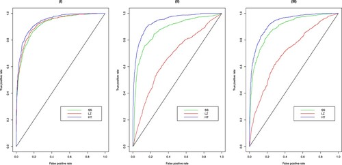
Table 2. Empirical size and power comparison at the 5% level with $n_1=n_2=15$ and p = 100, 200, 400, 800, 1200.

	$\rho =0.3$			$\rho =0.6$			$\rho =0.7$
p	HT	SS	LZ	HT	SS	LZ	HT	SS	LZ
Multivariate normal distribution
100	4.1	4.6	3.6	21	20	22	56	53	58
200	3.7	5.0	3.5	22	21	23	59	56	60
400	4.3	4.5	3.7	25	23	23	59	59	61
800	4.5	6.8	3.5	24	28	23	62	65	63
1200	5.2	13	4.6	24	37	24	62	69	62
Multivariate t-distribution
100	4.7	4.8	19	22	21	33	53	52	47
200	4.8	4.6	20	23	20	32	57	55	46
400	5.7	4.2	23	26	21	34	60	55	48
800	6.0	6.2	22	26	22	35	61	54	47
1200	6.4	8.4	22	25	25	37	63	57	51
Multivariate mixture normal distribution
100	4.2	4.6	22	25	22	35	54	55	50
200	4.8	5.9	20	21	26	32	56	58	48
400	5.8	6.3	23	26	25	36	59	60	50
800	5.6	9.1	24	26	32	37	59	69	51
1200	6.1	13	24	26	39	34	60	72	48

Table 3. Empirical size and power comparison at the 5% level with $n_1=n_2=20$ and p = 100, 200, 400, 800, 1200.

	$\rho =0.3$			$\rho =0.6$			$\rho =0.7$
p	HT	SS	LZ	HT	SS	LZ	HT	SS	LZ
Multivariate normal distribution
100	5.1	3.9	5.3	35	29	37	79	75	78
200	4.1	4.1	3.9	34	33	35	81	81	82
400	5.6	6.4	5.1	35	36	35	84	83	84
800	4.3	3.9	4.1	36	36	35	84	86	86
1200	4.2	2.6	2.8	35	37	36	86	84	82
Multivariate t-distribution
100	5.8	4.1	25	36	31	42	75	77	58
200	5.0	4.2	22	36	35	38	78	79	58
400	6.7	4.6	27	37	34	40	80	82	57
800	5.8	4.8	26	39	33	45	84	80	63
1200	4.8	4.4	26	37	34	46	83	81	63
Multivariate mixture normal distribution
100	6.5	4.2	25	36	31	45	78	76	61
200	5.1	4.3	26	36	33	42	79	78	61
400	5.9	5.0	24	38	36	43	82	85	60
800	5.2	7.1	25	37	40	43	83	85	62
1200	4.6	6.2	25	39	42	43	84	89	63

Table 4. Empirical size and power comparison at the 5% level with $n_1=n_2=30$ and p = 100, 200, 400, 800, 1200.

	$\rho =0.3$			$\rho =0.6$			$\rho =0.7$
p	HT	SS	LZ	HT	SS	LZ	HT	SS	LZ
Multivariate normal distribution
100	3.9	4.7	3.1	60	58	60	98	98	99
200	4.2	3.6	4.1	62	61	62	98	98	99
400	5.4	5.2	4.7	64	63	64	99	98	99
800	4.7	5.0	3.8	64	60	64	99	99	99
1200	6.2	5.8	5.1	68	65	66	99	99	99
Multivariate t-distribution
100	4.4	3.9	27	58	57	53	97	98	72
200	5.7	4.8	27	62	59	49	97	98	72
400	5.2	5.6	29	62	62	51	98	99	73
800	5.9	4.5	28	61	62	51	99	99	74
1200	6.4	5.6	29	64	61	50	99	99	73
Multivariate mixture normal distribution
100	4.6	5.8	27	59	58	54	97	97	77
200	5.8	6.2	24	60	62	50	98	99	75
400	5.7	6.2	25	62	62	54	98	99	77
800	5.6	7.3	26	63	63	53	98	99	77
1200	5.8	5.4	26	63	66	54	99	99	78

Next, we consider an alternative structure of the covariance matrices, i.e. ${\mathbf{\Sigma }}_i=\left(a_{ikl}\right)$ for each $i\in \{1,2\}$, where $a_{ikk}=1,a_{ik,k+1}=\frac{{\rho }_i+{\rho }_i^2}{1+2{\rho }_i^2},a_{k,k+2}=\frac{{\rho }_i}{1+2{\rho }_i^2}$for each $k\in \{1,\dots ,p\}$ and the remaining entries of ${\mathbf{\Sigma }}_i$ are all zeros. Note that ${\mathbf{\Sigma }}_i$ is the corresponding covariance matrix of $x_i$ following the MA$\left(2\right)$ model: $x_{it}=z_{it}+{\rho }_i{z}_{i,t-1}+{\rho }_i{z}_{i,t-2},$where $z_{it}$'s are i.i.d. random variables with mean zero and variance $\frac{1}{1+2{\rho }_i^2}$. Under the null hypothesis, we set ${\rho }_1={\rho }_2=0.7$, while under the alternative hypothesis, we set ${\rho }_1=0.7$ and ${\rho }_2=0.1$ for instance. The other settings are all the same as the above. Tables 5 and 6 report the empirical sizes and power of these three methods, respectively. Although Table 6 suggests that the performance of empirical power of the three methods is similar, Table 5 suggests that the abilities of LZ and SS to control the empirical size are weakening much more quickly than HT with the increase of p for fixed $n_1$ and $n_2$, especially when the dimension is comparable to or larger than the squares of the sample sizes.

Table 5. Empirical size comparison at the 5% level with the MA(2) covariance matrices with $n_1=n_2=15$, 20, 30 and p = 100, 200, 400, 800, 1200.

	$n_1=n_2=15$			$n_1=n_2=20$			$n_1=n_2=30$
p	HT	SS	LZ	HT	SS	LZ	HT	SS	LZ
Multivariate normal distribution
100	2.7	4.1	2.6	4.2	3.7	5.6	3.6	4.3	4.8
200	3.6	2.9	3.4	4.0	3.4	3.8	4.1	3.7	4.3
400	5.1	4.4	4.0	5.7	4.6	5.6	4.7	4.5	4.8
800	4.2	5.3	3.6	3.9	3.8	2.2	4.4	4.1	3.8
1200	5.8	7.8	5.8	3.1	5.6	3.0	3.9	4.3	6.6
Multivariate t-distribution
100	4.2	3.3	19	6.5	4.0	24	4.8	5.6	29
200	6.0	4.4	19	6.0	3.9	23	5.9	4.0	28
400	6.0	4.0	22	6.5	3.2	25	6.1	4.9	28
800	5.7	7.0	22	6.1	4.2	26	6.7	3.4	27
1200	6.7	7.8	23	6.1	4.9	26	6.9	5.1	30
Multivariate mixture normal distribution
100	5.0	3.5	22	5.6	3.7	27	4.8	3.5	26
200	5.7	4.0	25	6.3	4.1	26	6.3	4.4	27
400	5.8	5.8	23	6.3	4.3	28	6.2	3.2	26
800	5.4	7.0	24	5.1	7.0	26	5.9	4.7	26
1200	5.9	8.8	24	4.9	7.9	25	5.2	5.2	26

Table 6. Empirical power comparison at the 5% level with the MA(2) covariance matrices with $n_1=n_2=15$, 20, 30 and p = 100, 200, 400, 800, 1200.

	$n_1=n_2=15$			$n_1=n_2=20$			$n_1=n_2=30$
p	HT	SS	LZ	HT	SS	LZ	HT	SS	LZ
Multivariate normal distribution
100	42	40	44	65	63	66	92	92	93
200	42	41	43	67	64	67	93	93	94
400	45	44	48	67	66	68	94	94	94
800	44	47	41	66	68	67	93	93	94
1200	45	55	44	65	70	64	94	95	94
Multivariate t-distribution
100	42	40	40	65	62	56	91	92	67
200	42	40	42	64	63	50	91	92	67
400	43	40	46	64	66	51	92	92	65
800	44	45	46	64	64	51	91	94	65
1200	45	45	46	62	61	54	92	94	68
Multivariate mixture normal distribution
100	43	45	42	64	61	57	90	92	68
200	44	44	44	66	66	56	91	93	73
400	45	48	43	66	68	55	93	93	69
800	43	55	43	65	71	53	92	95	70
1200	43	61	46	62	74	53	92	94	66

Overall, the comprehensive numerical results suggest that the proposed HT test has obvious advantages in terms of controlling empirical size over the existing two methods. Such gain is especially clear when the original distribution deviates from normality, and when the dimension is larger than the squares of sample sizes.

4. Application

In this section, we apply the proposed testing method to a gene dataset, which contains the expression of the 2000 genes with the highest minimal intensity across the 62 tissues. Each entry in the dataset is a gene intensity derived using the filtering process proposed in Alon et al. (1999). The dataset was previously studied by Alon et al. (1999), and now can be freely downloaded at the following website: http://genomics-pubs.princeton.edu/oncology/affydata/index.html.

Among the 62 tissues, there are 22 normal tissues and 40 tumour colon tissues. We aim to test the hypothesis that the tissues in the tumour group and those in the normal group have the proportional covariance matrices in terms of the expression levels of the 2000 genes, where the dimension 2000 is larger than the squares of the sample sizes, 484 and 1600.

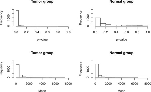
First, the normal distribution was tested for the expression data of each gene, using the Shapiro–Wilk test. The top two panels of Figure 1 present the histograms of the p-values of the normality tests for the tumour group and the normal group, respectively, which indicate that for a large number of genes the expression data are non-normal. In fact, under the significance level of 0.05, the overall rejection rates of all the normality tests are $93.55\mathrm{\%}$ and $37.75\mathrm{\%}$ for the tumour group and the normal group, respectively. This motivates us to use a nonparametric approach for testing the above hypothesis, which can deal with the high-dimensional data from non-normal distributions.

The bottom two panels of Figure 2 indicate that there exist some genes with very high values of sample mean in terms of expression. We see that the sample means vary largely for each of the two groups and recall that the dimension is larger than the squares of the sample sizes, which raises a concern that using a spatial sign-based approach may lead to an uncontrollable bias. Hence, in theory, a spatial rank-based approach is more appropriate for this dataset.

Figure 2. Histograms of the p-values of the normality tests and the gene expression means, for the tumour group and the normal group, respectively.

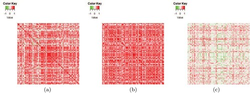
Based on the above reasons, we apply the proposed HT test to this dataset. The test statistic and p-value of the HT test are 4.823 and $0.000,$ respectively, hence the null hypothesis is rejected, which suggests that the covariance matrix of the gene expression levels of the tumour group is significantly not proportional to that of the normal group. This result can also be intuitively verified by comparing the sample correlation matrices of the two groups. As a convenience and for demonstration purposes, in Figure 3, we only plot the heatmaps of the sample correlation matrices of the two groups as well as the difference of the two matrices using the first 100 genes in the original data. The heatmaps demonstrate that there are some intuitive differences between the two sample correlation matrices, which tends to support our result of rejecting the null hypothesis.

Figure 3. Heatmaps of the sample correlation matrices of the two groups as well as the difference of the two matrices, which are constructed via the first 100 genes in the original data. (a) Normal group, (b) tumour group and (c) difference of two groups.

5. Conclusion

We have proposed the HT test, a new high-dimensional spatial rank test, for the proportionality testing problem of two high-dimensional covariance matrices, which is a high-dimensional extension of Kendall's tau test. It inherits the robustness advantage of the traditional spatial rank-based methods, and also has strong potential in dealing with the high-dimensional data, where the dimension can be potentially much larger than the squares of the sample sizes. We establish the asymptotic distributions of the proposed method rigorously. In comparison with some existing test procedures, the gain in empirical power and empirical size of HT is especially clear in high-dimensional and heavy-tailed data, shown by many numerical evidence. The real data analysis shows the applicability and pertinence of the proposed method to high-dimensional gene expression data.

Disclosure statement

No potential conflict of interest was reported by the author(s).

Additional information

Funding

This work was supported by the National Natural Science Foundation of China [Grant Numbers 11501092, 11571068] and the Special Fund for Key Laboratories of Jilin Province, China [Grant Number 20190201285JC].

Appendix

Define ${\mathbf{U}}_{\mathit{X},i}=U({\mathit{X}}_i-{\mathit{\theta }}_{\mathit{X}}),{\mathbf{U}}_{\mathit{Y},i}=U({\mathit{Y}}_i-{\mathit{\theta }}_{\mathit{Y}}).$Before proving the main theorem, below we recall some necessary lemmas.

Lemma A.1

Under Conditions (C1) and (C2), for any $p\times p$ symmetric matrix $\mathit{W}$, $\begin{array}{rl}\mathbb{E}\left\{\right({\mathbf{U}}_{\mathit{X},i}^{\mathrm{T}}{\mathbf{U}}_{\mathit{X},j}{)}^4\}& =O\left(1\right)E^2\left\{{\mathbf{U}}_{\mathit{X},i}^{\mathrm{T}}{\mathbf{U}}_{\mathit{X},j}{)}^2\right\},\\ \mathbb{E}\left\{\right({\mathbf{U}}_{\mathit{X},i}^{\mathrm{T}}\mathit{W}{\mathbf{U}}_{\mathit{X},i}{)}^2\}& =O\left(1\right)E^2\left({\mathbf{U}}_{\mathit{X},i}^{\mathrm{T}}\mathit{W}{\mathbf{U}}_{\mathit{X},i}\right),\\ \mathbb{E}\left\{\right({\mathbf{U}}_{\mathit{X},i}^{\mathrm{T}}\mathit{W}{\mathbf{U}}_{\mathit{X},j}{)}^2\}& =O\left(1\right)E^2\left({\mathbf{U}}_{\mathit{X},i}^{\mathrm{T}}\mathit{W}{\mathbf{U}}_{\mathit{X},j}\right).\end{array}$

Note that Lemma A.1 is the same as Lemma 1 of Wang et al. (2015).

Lemma A.2

Let ${\mathbf{U}}^{\ast }=(U_1^{\ast },\dots ,U_p^{\ast }{)}^{\mathrm{T}}$ be a random vector uniformly distributed on the unit sphere of ${\mathcal{R}}^p$, then we have that

1. $\mathbb{E}\left({\mathbf{U}}^{\ast }\right)=\mathbf{0}$, $\mathrm{C}\mathrm{o}\mathrm{v}\left({\mathbf{U}}^{\ast }\right)=p^{-1}{\mathbf{I}}_p$, $\mathbb{E}\left(U_k^{\ast 4}\right)=3p^{-1}(p+2{)}^{-1}$ and $\mathbb{E}\left(U_k^{\ast 2}{U}_l^{\ast 2}\right)=p^{-1}(p+2{)}^{-1}$ for each $k,l\in \{1,\dots ,p\}$ with $k\ne l;$

2. for any $p\times p$ symmetric matrix $\mathit{W}$, $E\left\{\right({\mathbf{U}}^{\ast \mathrm{T}}\mathit{W}{\mathbf{U}}^{\ast }{)}^2\}=p^{-1}(p+2{)}^{-1}\left\{{\mathrm{t}\mathrm{r}}^2\right(\mathit{W})+2\mathrm{t}\mathrm{r}({\mathit{W}}^2\left)\right\}$ and $E\left\{\right({\mathbf{U}}^{\ast \mathrm{T}}\mathit{W}{\mathbf{U}}^{\ast }{)}^4\}=p^{-2}(p+2{)}^{-2}\left\{3{\mathrm{t}\mathrm{r}}^2\right({\mathit{W}}^2)+6\mathrm{t}\mathrm{r}({\mathit{W}}^2\left)\right\}$.

In Lemma A.2, the first statement has been proved in Section 3.1 of Fang et al. (1990) and the second statement has been proved in Zou et al. (2014).

Now, we are ready to present the proof of Theorem 2.2. Then, the proof of Theorem 2.1 can be directly obtained.

Proof of Theorem  2.2:

Define $\begin{array}{rl}& {\mathit{V}}_{\mathit{X},i}\doteq \mathbb{E}\left\{U\right({\mathit{X}}_i-{\mathit{X}}_j\left)|{\mathit{X}}_i\right\},{\mathit{V}}_{\mathit{Y},i}\doteq \mathbb{E}\left\{U\right({\mathit{Y}}_i-{\mathit{Y}}_j\left)|{\mathit{Y}}_i\right\},\\ & {\mathit{W}}_{\mathit{Y},ij}\doteq U({\mathit{Y}}_i-{\mathit{Y}}_j)-{\mathit{V}}_{\mathit{Y},i}+{\mathit{V}}_{\mathit{Y},j},\\ & {\mathit{W}}_{\mathit{X},ij}\doteq U({\mathit{X}}_i-{\mathit{X}}_j)-{\mathit{V}}_{\mathit{X},i}+{\mathit{V}}_{\mathit{X},j},\\ & {\mathbf{B}}_1\doteq \mathbb{E}\left({\mathit{V}}_{\mathit{X},i}{\mathit{V}}_{\mathit{X},i}^{\mathrm{T}}\right),{\mathbf{B}}_2\doteq \mathbb{E}\left({\mathit{V}}_{\mathit{Y},i}{\mathit{V}}_{\mathit{Y},i}^{\mathrm{T}}\right).\end{array}$Hence we have that $\mathbb{E}\left({\mathit{V}}_{\mathit{X},i}^{\mathrm{T}}{\mathit{V}}_{\mathit{X},j}\right)=0$ and $\mathbb{E}\left({\mathit{V}}_{\mathit{X},i}^{\mathrm{T}}{\mathit{W}}_{\mathit{X},ij}\right)=0$. According to Lemma 1 in Feng and Liu (2017), we have that $\mathbb{E}\left({\mathit{W}}_{\mathit{X},ij}^{\mathrm{T}}{\mathit{W}}_{\mathit{X},ij}\right)\to 0$ as p goes to infinity and ${\mathbf{B}}_1=0.5{\mathrm{\S }}_1\{1+o(1\left)\right\}$. The same goes for ${\mathit{W}}_{\mathit{Y},ij}$ and ${\mathbf{B}}_2$. On this ground, by Lemma A.1, we have that $\begin{array}{rl}\mathbb{E}\left\{\right({\mathit{V}}_{\mathit{X},i}^{\mathrm{T}}{\mathit{V}}_{\mathit{X},j}{)}^4\}& =O\left(1\right)E^2\left\{\right({\mathit{V}}_{\mathit{X},i}^{\mathrm{T}}{\mathit{V}}_{\mathit{X},j}{)}^2\},\\ \mathbb{E}\left\{\right({\mathit{V}}_{\mathit{X},i}^{\mathrm{T}}\mathbf{A}{\mathit{V}}_{\mathit{X},i}{)}^2\}& =O\left(1\right)E^2\left({\mathit{V}}_{\mathit{X},i}^{\mathrm{T}}\mathbf{A}{\mathit{V}}_{\mathit{X},i}\right),\\ \mathbb{E}\left\{\right({\mathit{V}}_{\mathit{X},i}^{\mathrm{T}}\mathbf{A}{\mathit{V}}_{\mathit{X},j}{)}^2\}& =O\left(1\right)E^2\left({\mathit{V}}_{\mathit{X},i}^{\mathrm{T}}\mathbf{A}{\mathit{V}}_{\mathit{X},j}\right).\end{array}$As a result, the first part of $T_{\mathrm{H}\mathrm{T}}$ has the following decomposition: $\begin{array}{rl}& \frac{p}{n_1(n_1-1)(n_1-2)(n_1-3)}\sum ^{\ast }\left\{U\right({\mathit{X}}_i-{\mathit{X}}_j{)}^{\mathrm{T}}U({\mathit{X}}_k-{\mathit{X}}_l){\}}^2\\ & =\frac{4p}{n_1(n_1-1)}\sum ^{\ast }({\mathit{V}}_{\mathit{X},i}^{\mathrm{T}}{\mathit{V}}_{\mathit{X},j}{)}^2\\ & +\frac{2p}{n_1(n_1-1)(n_1-2)}\sum ^{\ast }({\mathit{V}}_{\mathit{X},i}^{\mathrm{T}}{\mathit{W}}_{\mathit{X},kl}{)}^2\\ & +\frac{p}{n_1(n_1-1)(n_1-2)(n_1-3)}\sum ^{\ast }({\mathit{W}}_{\mathit{X},ij}^{\mathrm{T}}{\mathit{W}}_{\mathit{X},kl}{)}^2\\ & \doteq J_1+J_2+J_3.\end{array}$According to Lemma A.2 and the fact that $\mathbb{E}\left({\mathit{W}}_{\mathit{X},ij}^{\mathrm{T}}{\mathit{W}}_{\mathit{X},ij}\right)\to 0$ as p goes to infinity, we similarly have that $\mathbb{E}\left(J_2^2\right)=o\left\{p^2{n}^{-3}\mathrm{t}\mathrm{r}\right({\mathrm{\S }}_1^2\left)\right\}=o\left({\sigma }_n^2\right)$ and $\mathbb{E}\left(J_3^2\right)=o\left(p^2{n}^{-4}\right)=o\left({\sigma }_n^2\right)$. Using the similar techniques, we can decompose the rest two parts of $T_{\mathrm{H}\mathrm{T}}$, hence conclude that $\begin{array}{rl}{T}_{\mathrm{H}\mathrm{T}}& =\frac{4p}{n_1(n_1-1)}\sum ^{\ast }({\mathit{V}}_{\mathit{X},i}^{\mathrm{T}}{\mathit{V}}_{\mathit{X},j}{)}^2\\ & +\frac{4p}{n_2(n_2-1)}\sum ^{\ast }({\mathit{V}}_{\mathit{Y},i}^{\mathrm{T}}{\mathit{V}}_{\mathit{Y},j}{)}^2\\ & -\frac{8p}{n_1{n}_2}\sum _{i=1}^{n_1}\sum _{j=1}^{n_2}({\mathit{V}}_{\mathit{X},i}^{\mathrm{T}}{\mathit{V}}_{\mathit{Y},j}{)}^2+o_p({\sigma }_n)\\ & \doteq p{A}_{n_1}+p{B}_{n_2}-2p{C}_{n_1,n_2}+o_p\left({\sigma }_n\right).\end{array}$Therefore, we have that $\begin{array}{rl}& \mathrm{v}\mathrm{a}\mathrm{r}\left(T_{\mathrm{H}\mathrm{T}}\right)/{\sigma }_n^2\\ & =p^2{\sigma }_n^{-2}\left\{\mathrm{v}\mathrm{a}\mathrm{r}\right(A_{n_1})+\mathrm{v}\mathrm{a}\mathrm{r}(B_{n_2})+4\mathrm{v}\mathrm{a}\mathrm{r}(C_{n_1,n_2})\\ & -4\mathrm{c}\mathrm{o}\mathrm{v}(A_{n_1},C_{n_1,n_2})-4\mathrm{c}\mathrm{o}\mathrm{v}(B_{n_2},C_{n_1,n_2})\}+o(1).\end{array}$Below we will consider each item in $\mathrm{v}\mathrm{a}\mathrm{r}\left(T_{\mathrm{H}\mathrm{T}}\right)/{\sigma }_n^2$ one by one. Before we can get the further expression of $\mathrm{v}\mathrm{a}\mathrm{r}\left(A_{n_1}\right)$, we need to study $\mathbb{E}\left(A_{n_1}^2\right)$ first. We have that $\begin{array}{rl}\mathbb{E}\left(A_{n_1}^2\right)& =\frac{16}{n_1^2(n_1-1{)}^2}\mathbb{E}\left[{\left\{\sum ^{\ast }\right({\mathit{V}}_{\mathit{X},i}^{\mathrm{T}}{\mathit{V}}_{\mathit{X},j}{)}^2\}}^2\right]\\ & =\frac{16}{n_1^2(n_1-1{)}^2}\left[2n_1\right(n_1-1\left)\mathbb{E}\right\{\left({\mathit{V}}_{\mathit{X},i}^{\mathrm{T}}{\mathit{V}}_{\mathit{X},j}{)}^4\right\}\\ & +4n_1(n_1-1)(n_1-2)\mathbb{E}\left\{\right({\mathit{V}}_{\mathit{X},i}^{\mathrm{T}}{\mathit{V}}_{\mathit{X},j}{)}^2\left({\mathit{V}}_{\mathit{X},i}^{\mathrm{T}}{\mathit{V}}_{\mathit{X},k}{)}^2\right\}\\ & +n_1(n_1-1)(n_1-2)(n_1-3)\\ & \times \mathbb{E}\left\{\right({\mathit{V}}_{\mathit{X},i}^{\mathrm{T}}{\mathit{V}}_{\mathit{X},j}{)}^2\left({\mathit{V}}_{\mathit{X},k}^{\mathrm{T}}{\mathit{V}}_{\mathit{X},l}{)}^2\right\}].\end{array}$Using the same proof techniques as in Cheng et al. (2018), we can get the following equations: $\begin{array}{rl}& \mathbb{E}\left\{\right({\mathit{V}}_{\mathit{X},i}^{\mathrm{T}}{\mathit{V}}_{\mathit{X},j}{)}^4\}\\ & =\frac{1}{4}{p}^2(p+2{)}^{-2}\{3{\mathrm{t}\mathrm{r}}^2\left({\mathbf{\Lambda }}_1^2\right)+6\mathrm{t}\mathrm{r}\left({\mathbf{\Lambda }}_1^4\right)\left\}\right\{1+o\left(1\right)\},\\ & \mathbb{E}\left\{\right({\mathit{V}}_{\mathit{X},i}^{\mathrm{T}}{\mathit{V}}_{\mathit{X},j}{)}^2\}\\ & =\frac{1}{2}\mathrm{t}\mathrm{r}\left({\mathrm{\S }}_1^2\right)\{1+o(1\left)\right\}=p^{-2}\mathrm{t}\mathrm{r}\left({\mathbf{\Lambda }}_1^2\right)\{1+o(1\left)\right\},\\ & \mathbb{E}\left\{\right({\mathit{V}}_{\mathit{X},i}^{\mathrm{T}}{\mathit{V}}_{\mathit{X},j}{)}^2\left({\mathit{V}}_{\mathit{X},i}^{\mathrm{T}}{\mathit{V}}_{\mathit{X},k}{)}^2\right\}\\ & =\frac{1}{4}{p}^{-3}(p+2{)}^{-1}\{{\mathrm{t}\mathrm{r}}^2\left({\mathbf{\Lambda }}_1^2\right)+2\mathrm{t}\mathrm{r}\left({\mathbf{\Lambda }}_1^4\right)\left\}\right\{1+o\left(1\right)\}.\end{array}$On this ground, we have that $\begin{array}{rl}& \mathrm{v}\mathrm{a}\mathrm{r}\left(A_{n_1}\right)\\ & =\{\frac{4}{n_1(n_1-1)}\frac{{\mathrm{t}\mathrm{r}}^2\left({\mathbf{\Lambda }}_1^2\right)}{p^2(p+2{)}^2}+\frac{8}{n_1}\frac{p\mathrm{t}\mathrm{r}\left({\mathbf{\Lambda }}_1^4\right)-{\mathrm{t}\mathrm{r}}^2\left({\mathbf{\Lambda }}_1^2\right)}{p^4(p+2)}\}\\ & \times \{1+o(1\left)\right\}.\end{array}$Similarly, we have that $\begin{array}{rl}& \mathrm{v}\mathrm{a}\mathrm{r}\left(B_{n_2}\right)\\ & =(\frac{4}{n_2(n_2-1)}\frac{{\mathrm{t}\mathrm{r}}^2\left({\mathbf{\Lambda }}_2^2\right)}{p^2(p+2{)}^2}+\frac{8}{n_2}\frac{p\mathrm{t}\mathrm{r}\left({\mathbf{\Lambda }}_2^4\right)-{\mathrm{t}\mathrm{r}}^2\left({\mathbf{\Lambda }}_2^2\right)}{p^4(p+2)})\\ & \times \{1+o(1\left)\right\},\\ & \mathrm{v}\mathrm{a}\mathrm{r}\left(C_{n_1,n_2}\right)\\ & =[\frac{2}{n_1{n}_2}\frac{{\mathrm{t}\mathrm{r}}^2\left({\mathbf{\Lambda }}_1{\mathbf{\Lambda }}_2\right)}{p^2(p+2{)}^2}+(\frac{2}{n_1}+\frac{2}{n_2})\\ & \times \frac{p\mathrm{t}\mathrm{r}\left\{\right({\mathbf{\Lambda }}_1{\mathbf{\Lambda }}_2{)}^2\}-{\mathrm{t}\mathrm{r}}^2({\mathbf{\Lambda }}_1{\mathbf{\Lambda }}_2)}{p^4(p+2)}]\{1+o(1\left)\right\},\\ & \mathrm{c}\mathrm{o}\mathrm{v}(A_{n_1},C_{n_1,n_2})\\ & =\left\{\frac{4}{n_1}\frac{p\mathrm{t}\mathrm{r}\left({\mathbf{\Lambda }}_1^3{\mathbf{\Lambda }}_2\right)-\mathrm{t}\mathrm{r}\left({\mathbf{\Lambda }}_1{\mathbf{\Lambda }}_2\right)\mathrm{t}\mathrm{r}\left({\mathbf{\Lambda }}_1^2\right)}{p^4(p+2)}\right\}\{1+o(1\left)\right\},\\ & \mathrm{c}\mathrm{o}\mathrm{v}(B_{n_2},C_{n_1,n_2})\\ & =\left\{\frac{4}{n_2}\frac{p\mathrm{t}\mathrm{r}\left({\mathbf{\Lambda }}_2^3{\mathbf{\Lambda }}_1\right)-\mathrm{t}\mathrm{r}\left({\mathbf{\Lambda }}_1{\mathbf{\Lambda }}_2\right)\mathrm{t}\mathrm{r}\left({\mathbf{\Lambda }}_2^2\right)}{p^4(p+2)}\right\}\{1+o(1\left)\right\}.\end{array}$To sum up, we conclude that $\mathrm{v}\mathrm{a}\mathrm{r}\left(T_{\mathrm{H}\mathrm{T}}\right)={\sigma }_n^2\{1+o(1\left)\right\}$.

Define a sequence of random variables $\{{\mathbf{z}}_1,\dots ,{\mathbf{z}}_{n_1+n_2}\}$ as follows: $\begin{array}{rl}{\mathbf{z}}_i& ={\mathit{V}}_{\mathit{X},i}\mathrm{f}\mathrm{o}\mathrm{r}\mathrm{e}\mathrm{a}\mathrm{c}\mathrm{h}i\in \{1,\dots ,n_1\}\mathrm{a}\mathrm{n}\mathrm{d}\\ {\mathbf{z}}_{n_1+j}& ={\mathit{V}}_{\mathit{Y},j}\mathrm{f}\mathrm{o}\mathrm{r}\mathrm{e}\mathrm{a}\mathrm{c}\mathrm{h}j\in \{1,\dots ,n_2\}.\end{array}$Let ${\mathbb{E}}_k(\cdot )$ denote the conditional expectation conditional on $\{{\mathbf{z}}_1,\dots ,{\mathbf{z}}_k\}$. Define $D_{n,k}=p^{-1}\left\{{\mathbb{E}}_k\right(T_{\mathrm{H}\mathrm{T}})-{\mathbb{E}}_{k-1}(T_{\mathrm{H}\mathrm{T}}\left)\right\}$, then $p^{-1}\{T_{\mathrm{H}\mathrm{T}}-\mathbb{E}(T_{\mathrm{H}\mathrm{T}}\left)\right\}=\sum _{k=1}^{n_1+n_2}{D}_{n,k}$. As a result, the sequence $\{D_{n,1},\dots ,D_{n,n_1+n_2}\}$ constitutes a martingale difference with respect to the σ-fields $\sigma ({\mathbf{z}}_1,{\mathbf{z}}_2,\dots ,{\mathbf{z}}_k)$. To use the martingale central limit theorem, we need to get the following results first: (A1) $\begin{array}{rl}& p^2\sum _{k=1}^{n_1+n_2}{\sigma }_{n,k}^2/\mathrm{v}\mathrm{a}\mathrm{r}\left(T_{\mathrm{H}\mathrm{T}}\right)⟹p1\mathrm{a}\mathrm{n}\mathrm{d}\\ & \sum _{k=1}^{n_1+n_2}\mathbb{E}\left(D_{nk}^4\right)=p^{-4}o\left\{{\mathrm{v}\mathrm{a}\mathrm{r}}^2\right(T_{\mathrm{H}\mathrm{T}}\left)\right\},\end{array}$(A1) where ${\sigma }_{n,k}^2\doteq {\mathbb{E}}_{k-1}\left(D_{n,k}^2\right)$.

Proof

Proof of the first part of (A1(A1) $\begin{array}{rl}& p^2\sum _{k=1}^{n_1+n_2}{\sigma }_{n,k}^2/\mathrm{v}\mathrm{a}\mathrm{r}\left(T_{\mathrm{H}\mathrm{T}}\right)⟹p1\mathrm{a}\mathrm{n}\mathrm{d}\\ & \sum _{k=1}^{n_1+n_2}\mathbb{E}\left(D_{nk}^4\right)=p^{-4}o\left\{{\mathrm{v}\mathrm{a}\mathrm{r}}^2\right(T_{\mathrm{H}\mathrm{T}}\left)\right\},\end{array}$(A1) )

As $\mathbb{E}\left(\sum _{k=1}^{n_1+n_2}{\sigma }_{n,k}^2\right)=p^{-2}\times \mathrm{v}\mathrm{a}\mathrm{r}\left(T_{\mathrm{H}\mathrm{T}}\right)$, we only need to show that as $min\{n_1,n_2\}\to \mathrm{\infty }$, $\mathrm{v}\mathrm{a}\mathrm{r}\left(\sum _{k=1}^{n_1+n_2}{\sigma }_{n,k}^2\right)=o\left\{p^{-4}{\mathrm{v}\mathrm{a}\mathrm{r}}^2\right(T_{\mathrm{H}\mathrm{T}}\left)\right\}$. Define ${\mathbf{\Gamma }}_{1,k-1}=\sum _{i=1}^{k-1}({\mathbf{z}}_i{\mathbf{z}}_i^{\mathrm{\prime }}-{\mathbf{B}}_1)$ for each $k\in \{1,\dots ,n_1-1\}$, and define ${\mathbf{\Gamma }}_{2,n_1+l-1}=\sum _{i=1}^{l-1}({\mathbf{z}}_{n_1+i}{\mathbf{z}}_{n_1+i}^{\mathrm{\prime }}-{\mathbf{B}}_2)$ for each $l\in \{1,\dots ,n_2-1\}$. For each $k\in \{1,\dots ,n_1\}$, we have that $\begin{array}{rl}& ({\mathbb{E}}_k-{\mathbb{E}}_{k-1})\left(A_{n_1}\right)\\ & =\frac{2}{n_1(n_1-1)}\{{\mathit{V}}_{\mathit{X},k}^{\mathrm{T}}{\mathbf{\Gamma }}_{1,k-1}{\mathit{V}}_{\mathit{X},k}-\mathrm{t}\mathrm{r}({\mathbf{\Gamma }}_{1,k-1}{\mathbf{B}}_1\left)\right\}\\ & +\frac{2}{n_1}\{{\mathit{V}}_{\mathit{X},k}^{\mathrm{T}}{\mathbf{B}}_1{\mathit{V}}_{\mathit{X},k}-\mathrm{t}\mathrm{r}({\mathbf{B}}_1^2\left)\right\},\end{array}$ $({\mathbb{E}}_k-{\mathbb{E}}_{k-1})\left(B_{n_2}\right)=0,$and $({\mathbb{E}}_k-{\mathbb{E}}_{k-1})\left(C_{n_1,n_2}\right)=\frac{1}{n_1}\{{\mathit{V}}_{\mathit{X},k}^{\mathrm{T}}{\mathbf{B}}_2{\mathit{V}}_{\mathit{X},k}-\mathrm{t}\mathrm{r}({\mathbf{B}}_1{\mathbf{B}}_2\left)\right\}.$For each $k\in \{n_1+1,\dots ,n_1+n_2\}$, we have that $({\mathbb{E}}_k-{\mathbb{E}}_{k-1})\left(A_{n_1}\right)=0,$ $\begin{array}{rl}& ({\mathbb{E}}_k-{\mathbb{E}}_{k-1})\left(B_{n_2}\right)\\ & =\frac{2}{n_2(n_2-1)}\{{\mathit{V}}_{\mathit{Y},k-n_1}^{\mathrm{T}}{\mathbf{\Gamma }}_{2,k-1}{\mathit{V}}_{\mathit{Y},k-n_1}-\mathrm{t}\mathrm{r}({\mathbf{\Gamma }}_{2,k-1}{\mathbf{B}}_2\left)\right\}\\ & +\frac{2}{n_2}\{{\mathit{V}}_{\mathit{Y},k-n_1}^{\mathrm{T}}{\mathbf{B}}_2{\mathit{V}}_{\mathit{Y},k-n_1}-\mathrm{t}\mathrm{r}({\mathbf{B}}_2^2\left)\right\},\end{array}$and $\begin{array}{rl}& ({\mathbb{E}}_k-{\mathbb{E}}_{k-1})\left(C_{n_1,n_2}\right)\\ & =\frac{1}{n_1{n}_2}\{{\mathit{V}}_{\mathit{Y},k-n_1}^{\mathrm{T}}\left(\sum _{i=1}^{n_1}{\mathit{V}}_{\mathit{X},i}{\mathit{V}}_{\mathit{X},i}^{\mathrm{T}}\right){\mathit{V}}_{\mathit{Y},k-n_1}\\ & -\mathrm{t}\mathrm{r}\left(\sum _{i=1}^{n_1}{\mathit{V}}_{\mathit{X},i}{\mathit{V}}_{\mathit{X},i}^{\mathrm{T}}{\mathbf{B}}_2\right)\}.\end{array}$Thus, for each $k\in \{1,\dots ,n_1\}$, $\begin{array}{rl}{\sigma }_{n,k}^2& ={\mathbb{E}}_{k-1}(\left[\frac{2}{n_1(n_1-1)}\right\{{\mathit{V}}_{\mathit{X},k}^{\mathrm{T}}{\mathbf{\Gamma }}_{1,k-1}{\mathit{V}}_{\mathit{X},k}-\mathrm{t}\mathrm{r}\left({\mathbf{\Gamma }}_{1,k-1}{\mathbf{B}}_1\right)\}\\ & +\frac{2}{n_1}\{{\mathit{V}}_{\mathit{X},k}^{\mathrm{T}}{\mathbf{B}}_1{\mathit{V}}_{\mathit{X},k}-\mathrm{t}\mathrm{r}({\mathbf{B}}_1^2\left)\right\}\\ & {-\frac{2}{n_1}\{{\mathit{V}}_{\mathit{X},k}^{\mathrm{T}}{\mathbf{B}}_2{\mathit{V}}_{\mathit{X},k}-\mathrm{t}\mathrm{r}({\mathbf{B}}_1{\mathbf{B}}_2\left)\right\}]}^2)\\ & =(\frac{8}{n_1^2(n_1-1{)}^2}\frac{p\mathrm{t}\mathrm{r}({\mathbf{\Gamma }}_{1,k-1}{\mathbf{\Lambda }}_1{)}^2-{\mathrm{t}\mathrm{r}}^2({\mathbf{\Gamma }}_{1,k-1}{\mathbf{\Lambda }}_1)}{p^2(p+2)}\\ & +\frac{16}{n_1^2(n_1-1)}\frac{p\mathrm{t}\mathrm{r}\left({\mathbf{\Gamma }}_{1,k-1}{\mathbf{\Lambda }}_1^3\right)-\mathrm{t}\mathrm{r}\left({\mathbf{\Gamma }}_{1,k-1}{\mathbf{\Lambda }}_1\right)\mathrm{t}\mathrm{r}\left({\mathbf{\Lambda }}_1^2\right)}{p^3(p+2)}\\ & -\frac{16}{n_1^2(n_1-1)}\\ & \times \frac{p\mathrm{t}\mathrm{r}\left({\mathbf{\Gamma }}_{1,k-1}{\mathbf{\Lambda }}_1{\mathbf{\Lambda }}_2{\mathbf{\Lambda }}_1\right)-\mathrm{t}\mathrm{r}\left({\mathbf{\Gamma }}_{1,k-1}{\mathbf{\Lambda }}_1\right)\mathrm{t}\mathrm{r}\left({\mathbf{\Lambda }}_1{\mathbf{\Lambda }}_2\right)}{p^3(p+2)}\\ & +\frac{8}{n_1^2}\frac{p\mathrm{t}\mathrm{r}\left[\right\{{\mathbf{\Lambda }}_1({\mathbf{\Lambda }}_1-{\mathbf{\Lambda }}_2){\}}^2]-{\mathrm{t}\mathrm{r}}^2\{{\mathbf{\Lambda }}_1({\mathbf{\Lambda }}_1-{\mathbf{\Lambda }}_2)\}}{p^4(p+2)})\\ & \times \{1+o(1\left)\right\},\end{array}$and for each $k\in \{n_1+1,\dots ,n_1+n_2\}$, $\begin{array}{rl}{\sigma }_{n,k}^2& ={\mathbb{E}}_{k-1}(\left[\frac{2}{n_2(n_2-1)}\right\{{\mathit{V}}_{\mathit{Y},k-n_1}^{\mathrm{T}}{\mathbf{\Gamma }}_{2,k-1}{\mathit{V}}_{\mathit{Y},k-n_1}\\ & -\mathrm{t}\mathrm{r}\left({\mathbf{\Gamma }}_{2,k-1}{\mathbf{B}}_2\right)\}\\ & +\frac{2}{n_2}\{{\mathit{V}}_{\mathit{Y},k-n_1}^{\mathrm{T}}{\mathbf{B}}_2{\mathit{V}}_{\mathit{Y},k-n_1}-\mathrm{t}\mathrm{r}({\mathbf{B}}_2^2\left)\right\}\\ & +\frac{2}{n_1{n}_2}\{{\mathit{V}}_{\mathit{Y},k-n_1}^{\mathrm{T}}\left(\sum _{i=1}^{n_1}{\mathit{V}}_{\mathit{X},i}{\mathit{V}}_{\mathit{X},i}^{\mathrm{T}}\right){\mathit{V}}_{\mathit{Y},k-n_1}\\ & {-\mathrm{t}\mathrm{r}\left(\sum _{i=1}^{n_1}{\mathit{V}}_{\mathit{X},i}{\mathit{V}}_{\mathit{X},i}^{\mathrm{T}}{\mathbf{B}}_2\right)\}]}^2)\\ & =[\phantom{\frac{\begin{array}{c}{\displaystyle p\mathrm{t}\mathrm{r}\left\{\right(\sum _{i=1}^{n_1}{\mathit{V}}_{\mathit{X},i}{\mathit{V}}_{\mathit{X},i}^{\mathrm{T}}{\mathbf{\Lambda }}_2{)}^2\}}\\ -{\mathrm{t}\mathrm{r}}^2({\mathbf{\Lambda }}_2{\displaystyle \sum _{i=1}^{n_1}{\mathit{V}}_{\mathit{X},i}{\mathit{V}}_{\mathit{X},i}^{\mathrm{T}})}\end{array}}{p^2(p+2)}}\frac{8}{n_2^2(n_2-1{)}^2}\frac{p\mathrm{t}\mathrm{r}({\mathbf{\Gamma }}_{2,k-1}{\mathbf{\Lambda }}_2{)}^2-{\mathrm{t}\mathrm{r}}^2({\mathbf{\Gamma }}_{2,k-1}{\mathbf{\Lambda }}_2)}{p^2(p+2)}\\ & +\frac{16}{n_2^2(n_2-1)}\frac{p\mathrm{t}\mathrm{r}\left({\mathbf{\Gamma }}_{2,k-1}{\mathbf{\Lambda }}_2^3\right)-\mathrm{t}\mathrm{r}\left({\mathbf{\Gamma }}_{2,k-1}{\mathbf{\Lambda }}_2\right)\mathrm{t}\mathrm{r}\left({\mathbf{\Lambda }}_2^2\right)}{p^3(p+2)}\end{array}$ $\begin{array}{r}-\frac{16}{n_1{n}_2^2(n_2-1)}\\ & \times \frac{{\displaystyle \mathrm{t}\mathrm{r}\left\{{\mathbf{\Gamma }}_{2,k-1}{\mathbf{\Lambda }}_2\right({\displaystyle \sum _{i=1}^{n_1}{\mathit{V}}_{\mathit{X},i}{\mathit{V}}_{\mathit{X},i}^{\mathrm{T}}\left){\mathbf{\Lambda }}_2\right\}}}}{p^2(p+2)}\\ & -\frac{\mathrm{t}\mathrm{r}\left({\mathbf{\Gamma }}_{2,k-1}{\mathbf{\Lambda }}_2\right)\mathrm{t}\mathrm{r}\left\{{\mathbf{\Lambda }}_2\right({\displaystyle \sum _{i=1}^{n_1}{\mathit{V}}_{\mathit{X},i}{\mathit{V}}_{\mathit{X},i}^{\mathrm{T}}\left)\right\}}}{p^2(p+2)}\\ & +\frac{8}{n_2^2}\frac{p\mathrm{t}\mathrm{r}\left({\mathbf{\Lambda }}_2^4\right)-{\mathrm{t}\mathrm{r}}^2\left({\mathbf{\Lambda }}_2^2\right)}{p^4(p+2)}\\ & -\frac{16}{n_1{n}_2^2}\frac{{\displaystyle p\mathrm{t}\mathrm{r}({\displaystyle \sum _{i=1}^{n_1}{\mathit{V}}_{\mathit{X},i}{\mathit{V}}_{\mathit{X},i}^{\mathrm{T}}{\mathbf{\Lambda }}_2^3)}}}{p^3(p+2)}\\ & -\frac{\mathrm{t}\mathrm{r}({\displaystyle \sum _{i=1}^{n_1}{\mathit{V}}_{\mathit{X},i}{\mathit{V}}_{\mathit{X},i}^{\mathrm{T}}{\mathbf{\Lambda }}_2\left)\mathrm{t}\mathrm{r}\right({\mathbf{\Lambda }}_2^2)}}{p^3(p+2)}\\ & +\frac{8}{n_1^2{n}_2^2}\frac{{\displaystyle p\mathrm{t}\mathrm{r}\left\{\right({\displaystyle \sum _{i=1}^{n_1}{\mathit{V}}_{\mathit{X},i}{\mathit{V}}_{\mathit{X},i}^{\mathrm{T}}{\mathbf{\Lambda }}_2{)}^2\}}}}{p^2(p+2)}\\ & -\frac{{\displaystyle {\mathrm{t}\mathrm{r}}^2({\mathbf{\Lambda }}_2{\displaystyle \sum _{i=1}^{n_1}{\mathit{V}}_{\mathit{X},i}{\mathit{V}}_{\mathit{X},i}^{\mathrm{T}})}}}{p^2(p+2)}]\{1+o(1\left)\right\}.\end{array}$Hence $\begin{array}{rl}& \sum _{k=1}^{n_1+n_2}{\sigma }_{n,k}^2=(R_1+R_2+R_3+R_4+R_5\\ & +R_6+R_6+R_7+C_0\left)\right\{1+o\left(1\right)\},\end{array}$where $C_0$ is a constant, and $\begin{array}{rl}{R}_1& =\sum _{k=1}^{n_1}\frac{8}{n_1^2(n_1-1{)}^2}\\ & \times \frac{p\mathrm{t}\mathrm{r}\left\{\right({\mathbf{\Gamma }}_{1,k-1}{\mathbf{\Lambda }}_1{)}^2\}-{\mathrm{t}\mathrm{r}}^2({\mathbf{\Gamma }}_{1,k-1}{\mathbf{\Lambda }}_1)}{p^2(p+2)},\\ R_2& =\sum _{l=1}^{n_2}\frac{8}{n_2^2(n_2-1{)}^2}\\ & \times \frac{p\mathrm{t}\mathrm{r}\left\{\right({\mathbf{\Gamma }}_{2,n_1+l-1}{\mathbf{\Lambda }}_2{)}^2\}-{\mathrm{t}\mathrm{r}}^2({\mathbf{\Gamma }}_{2,n_1+l-1}{\mathbf{\Lambda }}_2)}{p^2(p+2)},\\ R_3& =\sum _{k=1}^{n_1}\frac{16}{n_1^2(n_1-1)}\\ & \times [\frac{p\mathrm{t}\mathrm{r}\left\{{\mathbf{\Gamma }}_{1,k-1}\right({\mathbf{\Lambda }}_1^3-{\mathbf{\Lambda }}_1{\mathbf{\Lambda }}_2{\mathbf{\Lambda }}_1\left)\right\}}{p^3(p+2)},\\ & -\frac{\mathrm{t}\mathrm{r}\left({\mathbf{\Gamma }}_{1,k-1}{\mathbf{\Lambda }}_1\right)\mathrm{t}\mathrm{r}\left\{{\mathbf{\Lambda }}_1\right({\mathbf{\Lambda }}_1-{\mathbf{\Lambda }}_2\left)\right\}}{p^3(p+2)}],\\ R_4& =\sum _{l=1}^{n_2}\frac{16}{n_2^2(n_2-1)}\\ & \times \frac{p\mathrm{t}\mathrm{r}\left({\mathbf{\Gamma }}_{2,n_1+l-1}{\mathbf{\Lambda }}_2^3\right)-\mathrm{t}\mathrm{r}\left({\mathbf{\Gamma }}_{2,n_1+l-1}{\mathbf{\Lambda }}_2\right)\mathrm{t}\mathrm{r}\left({\mathbf{\Lambda }}_2^2\right)}{p^3(p+2)},\\ R_5& =-\sum _{l=1}^{n_2}\frac{16}{n_1{n}_2^2(n_2-1)}\end{array}$ $\begin{array}{r}\times [\frac{p\mathrm{t}\mathrm{r}\left\{{\mathbf{\Gamma }}_{2,n_1+l-1}{\mathbf{\Lambda }}_2\right({\displaystyle \sum _{i=1}^{n_1}{\mathit{V}}_{\mathit{X},i}{\mathit{V}}_{\mathit{X},i}^{\mathrm{T}}\left){\mathbf{\Lambda }}_2\right\}}}{p^2(p+2)}\\ & -\frac{\mathrm{t}\mathrm{r}\left({\mathbf{\Gamma }}_{2,n_1+l-1}{\mathbf{\Lambda }}_2\right)\mathrm{t}\mathrm{r}\left\{{\mathbf{\Lambda }}_2\right({\displaystyle \sum _{i=1}^{n_1}{\mathit{V}}_{\mathit{X},i}{\mathit{V}}_{\mathit{X},i}^{\mathrm{T}}\left)\right\}}}{p^2(p+2)}],\\ R_6& =\sum _{l=1}^{n_2}\frac{8}{n_1^2{n}_2^2}\frac{{\displaystyle p\mathrm{t}\mathrm{r}\left\{\right({\displaystyle \sum _{i=1}^{n_1}{\mathit{V}}_{\mathit{X},i}{\mathit{V}}_{\mathit{X},i}^{\mathrm{T}}{\mathbf{\Lambda }}_2{)}^2\}}}}{p^2(p+2)}\\ & -\frac{{\mathrm{t}\mathrm{r}}^2({\mathbf{\Lambda }}_2{\displaystyle \sum _{i=1}^{n_1}{\mathit{V}}_{\mathit{X},i}{\mathit{V}}_{\mathit{X},i}^{\mathrm{T}})}}{p^2(p+2)},\\ R_7& ={\displaystyle \sum _{l=1}^{n_2}-\frac{16}{n_1{n}_2^2}\frac{{\displaystyle p\mathrm{t}\mathrm{r}({\displaystyle \sum _{i=1}^{n_1}{\mathit{V}}_{\mathit{X},i}{\mathit{V}}_{\mathit{X},i}^{\mathrm{T}}{\mathbf{\Lambda }}_2^3)}}}{p^3(p+2)}}\\ & -\frac{\mathrm{t}\mathrm{r}({\displaystyle \sum _{i=1}^{n_1}{\mathit{V}}_{\mathit{X},i}{\mathit{V}}_{\mathit{X},i}^{\mathrm{T}}{\mathbf{\Lambda }}_2\left)\mathrm{t}\mathrm{r}\right({\mathbf{\Lambda }}_2^2)}}{p^3(p+2)}.\end{array}$Moreover, to calculate the order of $\mathrm{v}\mathrm{a}\mathrm{r}\left(R_1\right)$, we need to evaluate $\mathrm{v}\mathrm{a}\mathrm{r}\left[\sum _{k=1}^{n_1}{p}^{-2}\mathrm{t}\mathrm{r}\right\{\left({\mathbf{\Gamma }}_{1,k-1}{\mathbf{\Lambda }}_1{)}^2\right\}]$ . Since $\begin{array}{rl}& \mathbb{E}\left({\left[p^{-2}\sum _{k=1}^{n_1}\sum _{i=1}^{k-1}\sum _{j=1}^{k-1}\right\{({\mathit{V}}_{\mathit{X},i}^{\mathrm{T}}{\mathbf{\Lambda }}_1{\mathit{V}}_{\mathit{X},j}{)}^2-\mathrm{t}\mathrm{r}({\mathbf{\Lambda }}_1{\mathbf{B}}_1{)}^2\left\}\right]}^2\right)\\ & =p^{-4}\sum _{k=1}^{n_1}\sum _{m=1}^{n_1}\mathbb{E}\left[\sum _{i=1}^{k-1}\sum _{j=1}^{k-1}\right\{({\mathit{V}}_{\mathit{X},i}^{\mathrm{T}}{\mathbf{\Lambda }}_1{\mathit{V}}_{\mathit{X},j}{)}^2-\mathrm{t}\mathrm{r}({\mathbf{\Lambda }}_1{\mathbf{B}}_1{)}^2\}\\ & \times \sum _{l=1}^{m-1}\sum _{h=1}^{m-1}\left\{\right({\mathit{V}}_{\mathit{X},l}^{\mathrm{T}}{\mathbf{\Lambda }}_1{\mathit{V}}_{\mathit{X},h}{)}^2-\mathrm{t}\mathrm{r}\left({\mathbf{\Lambda }}_1{\mathbf{B}}_1{)}^2\right\}]\\ & \le n_1\sum _{k=1}^{n_1}(k-1{)}^2{p}^{-4}\mathbb{E}\{({\mathit{V}}_{\mathit{X},i}^{\mathrm{T}}{\mathbf{\Lambda }}_1{\mathit{V}}_{\mathit{X},j}{)}^4-{\mathrm{t}\mathrm{r}}^2({\mathbf{\Lambda }}_1{\mathbf{B}}_1{)}^2\}\\ & +n_1^2\sum _{k=1}^{n_1}(k-1{)}^2{p}^{-4}.\\ & \mathbb{E}\left\{\right({\mathit{V}}_{\mathit{X},i}^{\mathrm{T}}{\mathbf{\Lambda }}_1{\mathit{V}}_{\mathit{X},j}{)}^2({\mathit{V}}_{\mathit{X},i}^{\mathrm{T}}{\mathbf{\Lambda }}_1{\mathit{V}}_{\mathit{X},l}{)}^2-{\mathrm{t}\mathrm{r}}^2({\mathbf{\Lambda }}_1{\mathbf{B}}_1{)}^2\}\\ & =C_1{n}_1^4{p}^{-4}{p}^{-4}\left\{{\mathrm{t}\mathrm{r}}^2\right({\mathbf{\Lambda }}_1^4)+\mathrm{t}\mathrm{r}({\mathbf{\Lambda }}_1^8\left)\right\}\\ & +C_2{n}_1^5{p}^{-4}{p}^{-4}\left\{\mathrm{t}\mathrm{r}\right({\mathbf{\Lambda }}_1^8)-p^{-1}{\mathrm{t}\mathrm{r}}^2({\mathbf{\Lambda }}_1^4\left)\right\},\end{array}$where $C_1$ and $C_2$ are constants, we have that $\begin{array}{rl}\mathrm{v}\mathrm{a}\mathrm{r}\left(R_1\right)& \le C_1{n}_1^{-4}{p}^{-8}{\mathrm{t}\mathrm{r}}^2\left({\mathbf{\Lambda }}_1^2\right)\mathrm{t}\mathrm{r}\left({\mathbf{\Lambda }}_1^4\right)\\ & +C_2{n}_1^{-3}{p}^{-8}\mathrm{t}\mathrm{r}\left({\mathbf{\Lambda }}_1^4\right)\left\{\mathrm{t}\mathrm{r}\right({\mathbf{\Lambda }}_1^4)-p^{-1}{\mathrm{t}\mathrm{r}}^2({\mathbf{\Lambda }}_1^2\left)\right\}.\end{array}$Based on the fact that $\mathrm{t}\mathrm{r}\left({\mathbf{\Lambda }}_1^4\right)/{\mathrm{t}\mathrm{r}}^2\left({\mathbf{\Lambda }}_1^2\right)\to 0$ and the following inequality ${\mathrm{v}\mathrm{a}\mathrm{r}}^2\left(T_{\mathrm{H}\mathrm{T}}\right)\ge K\{\frac{{\mathrm{t}\mathrm{r}}^4\left({\mathbf{\Lambda }}_1^2\right)}{p^4{n}_1^4}+\frac{{\mathrm{t}\mathrm{r}}^4\left({\mathbf{\Lambda }}_2^2\right)}{p^4{n}_2^4}\}$for some constant K, we conclude that $p^4\mathrm{v}\mathrm{a}\mathrm{r}\left(R_1\right)/{\mathrm{v}\mathrm{a}\mathrm{r}}^2\left(T_{\mathrm{H}\mathrm{T}}\right)\to 0,$which indicates that $\mathrm{v}\mathrm{a}\mathrm{r}\left(R_1\right)=o\left\{p^{-4}{\mathrm{v}\mathrm{a}\mathrm{r}}^2\right(T_{\mathrm{H}\mathrm{T}}\left)\right\}$. By using similar techniques, we conclude that $\mathrm{v}\mathrm{a}\mathrm{r}\left(R_l\right)=o\{p^{-4}\times {\mathrm{v}\mathrm{a}\mathrm{r}}^2(T_{\mathrm{H}\mathrm{T}}\left)\right\}$ for each $l\in \{1,\dots ,7\}$, based on which we finally conclude that $\mathrm{v}\mathrm{a}\mathrm{r}\left(\sum _{k=1}^{n_1+n_2}{\sigma }_{n,k}^2\right)=o\left\{p^{-4}{\mathrm{v}\mathrm{a}\mathrm{r}}^2\right(T_{\mathrm{H}\mathrm{T}}\left)\right\}$.

Proof

Proof of the second part of (A1(A1) $\begin{array}{rl}& p^2\sum _{k=1}^{n_1+n_2}{\sigma }_{n,k}^2/\mathrm{v}\mathrm{a}\mathrm{r}\left(T_{\mathrm{H}\mathrm{T}}\right)⟹p1\mathrm{a}\mathrm{n}\mathrm{d}\\ & \sum _{k=1}^{n_1+n_2}\mathbb{E}\left(D_{nk}^4\right)=p^{-4}o\left\{{\mathrm{v}\mathrm{a}\mathrm{r}}^2\right(T_{\mathrm{H}\mathrm{T}}\left)\right\},\end{array}$(A1) )

For $1\le k\le n_1$, $\begin{array}{rl}& \sum _{k=1}^{n_1}\mathbb{E}\left(D_{nk}^4\right)\\ & =\sum _{k=1}^{n_1}\mathbb{E}(\left[\frac{2}{n_1(n_1-1)}\right\{{\mathit{V}}_{\mathit{X},k}^{\mathrm{T}}{\mathbf{\Gamma }}_{1,k-1}{\mathit{V}}_{\mathit{X},k}-\mathrm{t}\mathrm{r}\left({\mathbf{\Gamma }}_{1,k-1}{\mathbf{B}}_1\right)\}\\ & +\frac{2}{n_1}\{{\mathit{V}}_{\mathit{X},k}^{\mathrm{T}}{\mathbf{B}}_1{\mathit{V}}_{\mathit{X},k}-\mathrm{t}\mathrm{r}({\mathbf{B}}_1^2\left)\right\}\\ & {-\frac{2}{n_1}\{{\mathit{V}}_{\mathit{X},k}^{\mathrm{T}}{\mathbf{B}}_2{\mathit{V}}_{\mathit{X},k}-\mathrm{t}\mathrm{r}({\mathbf{B}}_1{\mathbf{B}}_2\left)\right\}]}^4)\\ & \le c_1\left\{n_1^{-3}{p}^{-8}\mathrm{t}\mathrm{r}\right[\left\{{\mathbf{\Lambda }}_1\right({\mathbf{\Lambda }}_1-{\mathbf{\Lambda }}_2\left){\}}^2\right]\left(\mathrm{t}\mathrm{r}\right[\left\{{\mathbf{\Lambda }}_1\right({\mathbf{\Lambda }}_1-{\mathbf{\Lambda }}_2\left){\}}^2\right]\\ & -p^{-1}{\mathrm{t}\mathrm{r}}^2\left\{{\mathbf{\Lambda }}_1\right({\mathbf{\Lambda }}_1-{\mathbf{\Lambda }}_2\left)\right\})+n_1^{-5}{p}^{-8}{\mathrm{t}\mathrm{r}}^4\left({\mathbf{\Lambda }}_1^2\right)\},\end{array}$where $c_1$ is some constant. Then $p^4\sum _{k=1}^{n_1+n_2}\mathbb{E}\left(D_{nk}^4\right)/{\mathrm{v}\mathrm{a}\mathrm{r}}^2\left(T_{\mathrm{H}\mathrm{T}}\right)\to 0.$ Similarly, for $n_1\le k\le n_1+n_2$, $\begin{array}{rl}& \sum _{k=n_1}^{n_1+n_2}\mathbb{E}\left(D_{nk}^4\right)\\ & \le c_2\left(n_1^{-1}{n}_2^{-4}{p}^{-8}{\mathrm{t}\mathrm{r}}^2\right({\mathbf{\Lambda }}_1{\mathbf{\Lambda }}_2\left)\mathrm{t}\mathrm{r}\right\{{\mathbf{\Lambda }}_2({\mathbf{\Lambda }}_1-{\mathbf{\Lambda }}_2){\}}^2\\ & \times \left[\mathrm{t}\mathrm{r}\right\{{\mathbf{\Lambda }}_2({\mathbf{\Lambda }}_1-{\mathbf{\Lambda }}_2){\}}^2\\ & -p^{-1}{\mathrm{t}\mathrm{r}}^2\left\{{\mathbf{\Lambda }}_2\right({\mathbf{\Lambda }}_1-{\mathbf{\Lambda }}_2\left)\right\}]+n_2^{-5}{p}^{-8}{\mathrm{t}\mathrm{r}}^4({\mathbf{\Lambda }}_2^2)\\ & +n_1^{-2}{n}_2^{-4}{p}^{-8}{\mathrm{t}\mathrm{r}}^4\left({\mathbf{\Lambda }}_1{\mathbf{\Lambda }}_2\right)),\end{array}$

where $c_2$ is some constant. Then we have that as $n_1,n_2\to \mathrm{\infty }$, $\frac{p^4\sum _{k=1}^{n_1+n_2}\mathbb{E}\left(D_{nk}^4\right)}{{\mathrm{v}\mathrm{a}\mathrm{r}}^2\left(T_{\mathrm{H}\mathrm{T}}\right)}\to 0.$By using the martingale central limit theorem (Hall & Hyde, 1980), we finally conclude that $\frac{T_{\mathrm{H}\mathrm{T}}-\mathbb{E}\left(T_{\mathrm{H}\mathrm{T}}\right)}{\mathrm{v}\mathrm{a}\mathrm{r}\left(T_{\mathrm{H}\mathrm{T}}\right)}⟹dN(0,1).$

Proof of Proposition  2.1:

Using the same techniques as in the proof of Theorem 2.1, we have that $\mathbb{E}\left({\mathbf{A}}_1\right)={\mathrm{t}\mathrm{r}}^2\left({\mathrm{\S }}_1\right)$ and $\begin{array}{rl}\mathrm{V}\mathrm{a}\mathrm{r}\left\{\frac{p^2{\mathbf{A}}_1}{\mathrm{t}\mathrm{r}\left({\mathbf{\Lambda }}_1^2\right)}\right\}& =O(\frac{p^4}{{\mathrm{t}\mathrm{r}}^2{\mathbf{\Lambda }}_1^2}[\frac{2}{n_1(n_1-1)}\\ & \times \{\frac{3{\mathrm{t}\mathrm{r}}^2\left({\mathbf{\Lambda }}_1^2\right)+6\mathrm{t}\mathrm{r}\left({\mathbf{\Lambda }}_1^4\right)}{p^2(p+2{)}^2}-\frac{{\mathrm{t}\mathrm{r}}^2\left({\mathbf{\Lambda }}_1^2\right)}{p^4}\}]).\end{array}$Therefore, $\frac{p^2{\mathbf{A}}_1}{\mathrm{t}\mathrm{r}\left({\mathbf{\Lambda }}_1^2\right)}\to 1$, and similarly, $\frac{p^2{\mathbf{A}}_2}{\mathrm{t}\mathrm{r}\left({\mathbf{\Lambda }}_2^2\right)}\to 1$, hence $\frac{{\hat{\sigma }}_{0,n}^2}{{\sigma }_{0,n}^2}\to 1$.

References

- Alon, U., Barkai, N., Notterman, D. A., Gish, K., Ybarra, S., & Levine, D. M. J. (1999). Broad patterns of gene expression revealed by clustering analysis of tumor and normal colon tissues probed by oligonucleotide arrays. Proceedings of the National Academy of Sciences of the United States of America, 96(12), 6745–6750. https://doi.org/https://doi.org/10.1073/pnas.96.12.6745
- Bai, Z., & Saranadasa, H. (1996). Effect of high dimension: By an example of a two sample problem. Statistica Sinica, 6(2), 311–329.
- Barber, R. F., & Kolar, M. (2018). Rocket: Robust confidence intervals via Kendall's tau for transelliptical graphical models. The Annals of Statistics, 46(6B), 3422–3450. https://doi.org/https://doi.org/10.1214/17-AOS1663
- Bühlmann, P, & van de Geer, S. (2011). Statistics for High-dimensional Data: Methods, Theory and Applications (1st ed.). Springer Publishing Company, Incorporated.
- Cai, T. T., & Zhang, A. (2016). Inference for high-dimensional differential correlation matrices. Journal of Multivariate Analysis, 143(6009), 107–126. https://doi.org/https://doi.org/10.1016/j.jmva.2015.08.019
- Chen, S. X., & Qinm, Y. L. (2010). A two-sample test for high-dimensional data with applications to gene-set testing. Annals of Statistics, 38(2), 808–835.https://doi.org/https://doi.org/10.1214/09-AOS716
- Cheng, G., Liu, B., Peng, L., Zhang, B., & Zheng, S. (2018). Testing the equality of two high-dimensional spatial sign covariance matrices. Scandinavian Journal of Statistics, 46(1), 257–271. https://doi.org/https://doi.org/10.1111/sjos.v46.1
- Eriksen, P. S. (1987). Proportionality of covariance matrices. Annals of Statistics, 15(2), 732–748. https://doi.org/https://doi.org/10.1214/aos/1176350372
- Fang, K. T., Kotz, S., & Ng, K. W. (1990). Symmetric Multivariate and Related Distributions. Chapman and Hall.
- Federer, W. T. (1951). Testing proportionality of covariance matrices. Annals of Mathematical Statistics, 22(1), 102–106. https://doi.org/https://doi.org/10.1214/aoms/1177729697
- Feng, L., & Liu, B. (2017). High-dimensional rank tests for sphericity. Journal of Multivariate Analysis, 155, 217–233. https://doi.org/https://doi.org/10.1016/j.jmva.2017.01.003
- Feng, L., & Sun, F. (2016). Spatial-sign based high-dimensional location test. Electronic Journal of Statistics, 10(2), 2420–2434. https://doi.org/https://doi.org/10.1214/16-EJS1176
- Feng, L., Zou, C., & Wang, Z. (2016). Multivariate-sign-based high-dimensional tests for the two-sample location problem. Journal of the American Statistical Association, 111(514), 721–735. https://doi.org/https://doi.org/10.1080/01621459.2015.1035380
- Flury, B. K. (1986). Proportionality of k covariance matrices. Statistics and Probability Letters, 4(1), 29–33. https://doi.org/https://doi.org/10.1016/0167-7152(86)90035-0
- Flury, B. K., & Riedwyl, H. (1988). Multivariate Statistics: A Practical Approach. Chapman and Hall.
- Hall, P. G., & Hyde, C. C. (1980). Martingale Central Limit Theory and Its Applications. Academic Press.
- Han, F., Chen, S., & Liu, H. (2017). Distribution-free tests of independence in high dimensions. Biometrika, 104(4), 813–828. https://doi.org/https://doi.org/10.1093/biomet/asx050
- Han, F., & Liu, H. (2018). ECA: High-dimensional elliptical component analysis in non-Gaussian distributions. Journal of the American Statistical Association, 113(521), 252–268. https://doi.org/https://doi.org/10.1080/01621459.2016.1246366
- Kim, D. Y. (1971). Statistical inference for constants of proportionality between covariance matrices. Technical Report 59, Stanford University.
- Leung, D., & Drton, M. (2018). Testing independence in high dimensions with sums of rank correlations. The Annals of Statistics, 46(1), 280–307. https://doi.org/https://doi.org/10.1214/17-AOS1550
- Li, J., & Chen, S. X. (2012). Two sample tests for high dimensional covariance matrices. Annals of Statistics, 40(2), 908–940.https://doi.org/https://doi.org/10.1214/12-AOS993
- Liu, B., Xu, L., Zheng, S., & Tian, G. (2014). A new test for the proportionality of two large-dimensional covariance matrices. Journal of Multivariate Analysis, 131(1), 293–308. https://doi.org/https://doi.org/10.1016/j.jmva.2014.06.008
- Magyar, A., & Tyler, D. (2014). The asymptotic inadmissibility of the spatial sign covariance matrix for elliptically symmetric distributions. Biometrika, 101(3), 673–688. https://doi.org/https://doi.org/10.1093/biomet/asu020
- Mottonen, J., & Oja, H. (1995). Multivariate spatial sign and rank methods. Journal of Nonparametric Statistics, 5(2), 201–213. https://doi.org/https://doi.org/10.1080/10485259508832643
- Oja, H. (2010). Multivariate nonparametric methods with R. Springer.
- Rao, C. R. (1983). Likelihood ratio tests for relationships between two covariance matrices. In S. Karlin, T. Amemiya, & L. A. Goodman (Eds.), Studies in Econometrics, Time Series and Multivariate Statistics (pp. 529–543). Academic Press.
- Schott, J. R. (1991). Some tests for common principal component subspaces in several groups. Biometrika, 78(4), 771–777. https://doi.org/https://doi.org/10.1093/biomet/78.4.771
- Schott, J. R. (1999). A test for proportional covariance matrices. Computational Statistics and Data Analysis, 32(2), 135–146. https://doi.org/https://doi.org/10.1016/S0167-9473(99)00032-8
- Wang, L., Peng, B., & Li, R. (2015). A high-dimensional nonparametric multivariate test for mean vector. Journal of the American Statistical Association, 110(512), 1658–1669. https://doi.org/https://doi.org/10.1080/01621459.2014.988215
- Xu, L., Liu, B., Zheng, S., & Bao, S. (2014). Testing proportionality of two large-dimensional covariance matrices. Computational Statistics and Data Analysis, 78, 43–55. https://doi.org/https://doi.org/10.1016/j.csda.2014.03.014
- Zou, C. L., Peng, L. H., Feng, L., & Wang, Z. J. (2014). Multivariate sign-based high-dimensional tests for sphericity. Biometrika, 101(1), 229–236. https://doi.org/https://doi.org/10.1093/biomet/ast040
Appendix
Define
Before proving the main theorem, below we recall some necessary lemmas.
Lemma A.1
Under Conditions (C1) and (C2), for any symmetric matrix