Generalized fiducial methods for testing quantitative trait locus effects in genetic backcross studies

Abstract

In this paper, we propose generalized fiducial methods and construct four generalized p-values to test the existence of quantitative trait locus effects under phenotype distributions from a location-scale family. Compared with the likelihood ratio test based on simulation studies, our methods perform better at controlling type I errors while retaining comparable power in cases with small or moderate sample sizes. The four generalized fiducial methods support varied scenarios: two of them are more aggressive and powerful, whereas the other two appear more conservative and robust. A real data example involving mouse blood pressure is used to illustrate our proposed methods.

Keywords:

• Generalized fiducial inference
• quantitative trait locus
• mixture model
• Gibbs algorithm
• likelihood ratio test

1. Introduction

In medical and biological genetic research, quantitative trait locus (QTL) mapping is important in studies of the traits of all types of organisms. For example, QTLs can be identified and mapped to analyse the genetic factors contributing to blood pressure in animals (Sugiyama et al., 2001) or to the length of rice grains (Huang et al., 1997; R. Wu et al., 2007). As a standard process at the beginning of QTL mapping studies, tests for the existence of QTL effects – that is, whether the gene related to the traits is on the specified chromosome – should be deployed.

Interval mapping, proposed by Lander and Botstein (1989), is a popular method for detecting QTLs. Suppose that a putative QTL, denoted by Q, is located between the left and right flanking markers, M and N, in a backcross design. For individuals in the backcross population, the possible genotypes are MM and Mm at M, NN and Nn at N, and QQ and Qq at Q. Hence, the individuals in the backcross population have four marker genotypes: MM/NN, Mm/NN, MM/Nn, and Mm/Nn, where Mm/NN and MM/Nn are recombinant types. For each individual, M and N can be observed but Q cannot. A testing method based on these data for detecting a QTL in the interval M–N is referred to the interval mapping method.

Let r, $r_1$, and $r_2$ be the recombination frequencies – that is, the proportions of recombinant genotypes – between M and N, between M and Q, and between Q and N, respectively. In this paper, we only consider backcross designs without double recombination or interference between two-marker-QTL intervals, i.e., $r=r_1+r_2$ (R. Wu et al., 2007). Denote by C the coding variable for the genotypes at the two markers, with C = 1, 2, 3, 4 representing the genotypes MM/NN, Mm/NN, MM/Nn, and Mm/Nn, respectively. The probabilities of QTL genotypes are shown in Table 1; see also Chen and Chen (2005), R. Wu et al. (2007) and Zhang et al. (2008).

Table 1. Probabilities of QTL genotypes.

	C	$Pr(C=i)$	$Pr\left(QQ\right|C=i)$	$Pr\left(Qq\right|C=i)$
MM/NN	1	$(1-r)/2$	1	0
Mm/NN	2	r/2	$r_1/r$	$r_2/r$
MM/Nn	3	r/2	$r_2/r$	$r_1/r$
Mm/Nn	4	$(1-r)/2$	0	1

Let $f_1$ and $f_2$ be the phenotype density functions corresponding to two QTL genotypes QQ and Qq. Denote by $\{Y_{11},\dots ,Y_{1n_1}\}$, $\{Y_{21},\dots ,Y_{2n_2}\}$, $\{Y_{31},\dots ,Y_{3n_3}\}$, and $\{Y_{41},\dots ,Y_{4n_4}\}$ the phenotype data corresponding to the marker genotypes MM/NN, Mm/NN, MM/Nn, and Mm/Nn, respectively. Then, we have the following statistical model under the considered background: (1) $\begin{array}{rl}{Y}_{1j}& \sim f_1\left(y\right),j=1,\dots ,n_1,\\ Y_{2j}& \sim \theta f_1\left(y\right)+(1-\theta )f_2\left(y\right),j=1,\dots ,n_2,\\ Y_{3j}& \sim (1-\theta )f_1\left(y\right)+\theta f_2\left(y\right),j=1,\dots ,n_3,\\ Y_{4j}& \sim f_2\left(y\right),j=1,\dots ,n_4,\end{array}$(1) where $\theta =r_1/r$ and $y_{ij}$ are trait values corresponding to C = i, $i=1,\dots ,4$, $j=1,\dots ,n_i$. Here, r is known, as the two markers M and N are pre-specified, whereas $r_1$ and $r_2$ are unknown as the location of Q is unknown. Then, $\{Y_{2j},j=1,\dots ,n_2\}$ and $\{Y_{3j},j=1,\dots ,n_3\}$ are modelled by mixture distributions because of the recombination of non-sister chromatids in these individuals. Denoting the total sample size by $n=\sum _{i=1}^4{n}_i$, we have $n_i/n\to Pr(C=i)$ when each $n_i$ tends to ∞ at the same rate (R. Wu et al., 2007).

Under model (1(1) $\begin{array}{rl}{Y}_{1j}& \sim f_1\left(y\right),j=1,\dots ,n_1,\\ Y_{2j}& \sim \theta f_1\left(y\right)+(1-\theta )f_2\left(y\right),j=1,\dots ,n_2,\\ Y_{3j}& \sim (1-\theta )f_1\left(y\right)+\theta f_2\left(y\right),j=1,\dots ,n_3,\\ Y_{4j}& \sim f_2\left(y\right),j=1,\dots ,n_4,\end{array}$(1) ), testing the existence of QTL effects is equivalent to testing the null hypothesis: (2) $H_0:f_1=f_2.$(2) The null hypothesis in (2(2) $H_0:f_1=f_2.$(2) ) means that there are no QTL effects. In the literature, parametric methods are usually applied by assuming the specific distributions of $f_1$ and $f_2$. For example, Chen and Chen (2005) and Zhang et al. (2008) assume that $f_1$ and $f_2$ have normal distributions with the same variance, although in fact a QTL effect in variance may be more crucial (Korol et al., 1996; Liu et al., 2020). Recently, Liu et al. (2020) extended the likelihood ratio (LR) test to detect QTL effects where $f_1$ and $f_2$ are from a general location-scale family with unknown locations and/or scales, i.e., $f_k\left(y\right)=f(y;{\mu }_k,{\sigma }_k)$ with $f(y;\mu ,\sigma )=f\left(\right(y-\mu )/\sigma ;0,1)/\sigma$. Here, $f(\cdot ;0,1)$ is a known probability density function, and μ and σ are the location and scale parameters, respectively. Then, the hypothesis test problem in (2(2) $H_0:f_1=f_2.$(2) ) is transformed into: (3) $H_0:({\mu }_1,{\sigma }_1)=({\mu }_2,{\sigma }_2).$(3) In particular, under the assumption that ${\sigma }_1={\sigma }_2=\sigma$, the testing problem in (3(3) $H_0:({\mu }_1,{\sigma }_1)=({\mu }_2,{\sigma }_2).$(3) ) becomes (4) $H_0:{\mu }_1={\mu }_2.$(4) For the null hypotheses (3(3) $H_0:({\mu }_1,{\sigma }_1)=({\mu }_2,{\sigma }_2).$(3) ) and (4(4) $H_0:{\mu }_1={\mu }_2.$(4) ), Liu et al. (2020) proposed explicit representations of the limiting distribution of LR statistics and obtained more accurate asymptotic p-values than those of Rebai et al. (1994, 1995). The LR test in Liu et al. (2020) was shown to be more powerful than the Kolmogorov–Smirnov test and Anderson–Darling test. However, we found that the LR test inflated type I errors when the sample size was small or moderate, as shown in our simulation study in Section 3.

Based on the above discussion, it is desirable to develop new methods that control type I errors more accurately while retaining powerful performance with small or moderate sample sizes. One efficient method is the generalized fiducial inference developed by Hannig et al. (2006) and Hannig (2009), which constructs generalized p-values for the null hypotheses (3(3) $H_0:({\mu }_1,{\sigma }_1)=({\mu }_2,{\sigma }_2).$(3) ) and (4(4) $H_0:{\mu }_1={\mu }_2.$(4) ) under a fiducial inference frame introduced by Fisher (1930). In the literature, the generalized fiducial inference is widely applied in homogeneous data, i.e., assuming that all labels of samples are known. Recent research includes Lai et al. (2015), Hannig et al. (2016), Li et al. (2018), Cui and Hannig (2019), and Williams and Hannig (2019). However, generalized fiducial inference has not received much attention as a means of testing QTL effects under model (1(1) $\begin{array}{rl}{Y}_{1j}& \sim f_1\left(y\right),j=1,\dots ,n_1,\\ Y_{2j}& \sim \theta f_1\left(y\right)+(1-\theta )f_2\left(y\right),j=1,\dots ,n_2,\\ Y_{3j}& \sim (1-\theta )f_1\left(y\right)+\theta f_2\left(y\right),j=1,\dots ,n_3,\\ Y_{4j}& \sim f_2\left(y\right),j=1,\dots ,n_4,\end{array}$(1) ). In this paper, generalized fiducial inference is applied by constructing four types of generalized p-values to test the null hypotheses (3(3) $H_0:({\mu }_1,{\sigma }_1)=({\mu }_2,{\sigma }_2).$(3) ) and (4(4) $H_0:{\mu }_1={\mu }_2.$(4) ). Our methods have two advantages. (i) They can control type I errors more accurately than LR methods, especially for small and moderate sample sizes, although they may not be optimal in a conventional sense. (ii) They retain power comparable with or even greater than that of the LR methods.

The remainder of this article is organized as follows. In Section 2, four generalized fiducial methods are proposed for the null hypothesis (3(3) $H_0:({\mu }_1,{\sigma }_1)=({\mu }_2,{\sigma }_2).$(3) ). In Section 3, we develop comparisons of these proposed methods with the method of Liu et al. (2020) through simulated examples. In addition, a real genetic dataset is analysed by applying our methods in Section 4. Finally, Section 5 concludes the article. The proof of Theorem 2.1 and additional comparisons among some generalized pivotal quantities (GPQs) are provided in the supplementary material.

2. New test

The generalized fiducial inference is one of the most important ways to construct generalized p-values. In the following, we explain the general procedure proposed by Li et al. (2007, 2018) for obtaining generalized p-values based on a data-generating equation (DGE).

Let $\mathit{Y}$ be a random vector following a known distribution $F_{\mathit{\delta }}(\cdot )$, where $\mathit{\delta }$ is an unknown parameter vector. Suppose $\mathit{\xi }=\mathit{\xi }\left(\mathit{\delta }\right)=({\xi }_1,{\mathit{\xi }}_2^{\mathrm{T}}{)}^{\mathrm{T}}$, where ${\xi }_1$ is the parameter of interest and ${\mathit{\xi }}_2$ is the nuisance parameter vector. An observation of $\mathit{Y}$ is denoted by $\mathit{y}$. Suppose we have the DGE $\mathit{Y}=\mathit{G}(\mathit{\delta },\mathit{E}),$where $\mathit{E}$ is a random variable that has a known distribution. The observed version of DGE $\mathit{y}=\mathit{G}(\mathit{\delta },\mathit{e})$ has a unique solution for $\mathit{\delta }$, i.e., ${\mathit{G}}^{-1}(\mathit{y},\mathit{e})$. Then, the random quantities ${\mathit{G}}^{-1}(\mathit{y},\mathit{E})$ and $\mathit{\xi }\left({\mathit{G}}^{-1}\right(\mathit{y},\mathit{E}\left)\right)$ are the GPQs of $\mathit{\delta }$ and $\mathit{\xi }\left(\mathit{\delta }\right)$, and the distributions of ${\mathit{G}}^{-1}(\mathit{y},\mathit{E})$ and $\mathit{\xi }\left({\mathit{G}}^{-1}\right(\mathit{y},\mathit{E}\left)\right)$ are the fiducial distributions of $\mathit{\delta }$ and $\mathit{\xi }\left(\mathit{\delta }\right)$. Furthermore, if $\mathit{y}=\mathit{G}(\mathit{\delta },\mathit{e})$ has a unique solution for any $\mathit{e}$ and $\mathit{y}$, ${\xi }_1-{\xi }_1\left({\mathit{G}}^{-1}\right(\mathit{y},\mathit{E}\left)\right)$ is a generalized test variable of ${\xi }_1$, so that the generalized p-value for the one-sided hypothesis $H_0:{\xi }_1\le {\xi }_{10}\leftrightarrow H_1:{\xi }_1>{\xi }_{10}$ is $p=Pr\left({\xi }_1\right({\mathit{G}}^{-1}(\mathit{y},\mathit{E}))<{\xi }_{10})$.

Denote by $T_{\mathit{\delta }}=(T_{\theta },T_{{\mu }_1},T_{{\mu }_2},T_{{\sigma }_1},T_{{\sigma }_2}{)}^{\mathrm{T}}$ the GPQ of the parameter vector $\mathit{\delta }=(\theta ,{\mu }_1,{\mu }_2,{\sigma }_1,{\sigma }_2{)}^{\mathrm{T}}$. Based on the ideas of the above methods, if $T_{\mathit{\delta }}$ can be obtained by fiducial inference, we can find the GPQs of the parameters of interest ${\xi }_1={\mu }_2-{\mu }_1$ and ${\xi }_{1^{\prime }}={\sigma }_2-{\sigma }_1$, denoted by $T_{{\xi }_1}=T_{{\mu }_2}-T_{{\mu }_1}$ and $T_{{\xi }_{1^{\prime }}}=T_{{\sigma }_2}/T_{{\sigma }_1}$. Thus, the generalized p-values for the hypotheses ${\mu }_2-{\mu }_1=0$ and ${\sigma }_2/{\sigma }_1=1$ are (5) $p_1=2min\{Pr(T_{{\mu }_2}-T_{{\mu }_1}<0),Pr(T_{{\mu }_2}-T_{{\mu }_1}>0\left)\right\}$(5) and (6) $p_2=2min\{Pr(T_{{\sigma }_2}/T_{{\sigma }_1}<1),Pr(T_{{\sigma }_2}/T_{{\sigma }_1}>1\left)\right\}.$(6) According to Theorem 2.1 in Section 2.1, $p_1$ and $p_2$ follow the standard uniform distribution $U(0,1)$ independently. Then, according to Fisher's combined method (Fisher, 1932), the generalized p-value for testing the hypothesis in (3(3) $H_0:({\mu }_1,{\sigma }_1)=({\mu }_2,{\sigma }_2).$(3) ) is (7) $p_{\mathrm{G}\mathrm{V}}=Pr\{{\chi }_4^2>-2\log (p_1{p}_2\left)\right\}.$(7) For a given significance level α, the null hypothesis (3(3) $H_0:({\mu }_1,{\sigma }_1)=({\mu }_2,{\sigma }_2).$(3) ) is rejected if $p_{\mathrm{G}\mathrm{V}}\le \alpha$. Similarly, under the condition ${\sigma }_1={\sigma }_2=\sigma$, the generalized p-value for the hypothesis test problem in (4(4) $H_0:{\mu }_1={\mu }_2.$(4) ) becomes (8) $\begin{array}{rl}{\overline{p}}_{\mathrm{G}\mathrm{V}}& =2min\{Pr({\overline{T}}_{{\mu }_2}-{\overline{T}}_{{\mu }_1}<0),\\ & Pr({\overline{T}}_{{\mu }_2}-{\overline{T}}_{{\mu }_1}>0)\},\end{array}$(8) where ${\overline{T}}_{{\mu }_k}$ is the GPQ of ${\mu }_k$ (k = 1, 2) under same-scale conditions. The null hypothesis (4(4) $H_0:{\mu }_1={\mu }_2.$(4) ) is rejected if ${\overline{p}}_{\mathrm{G}\mathrm{V}}\le \alpha$.

For the mixture distribution frame in (1(1) $\begin{array}{rl}{Y}_{1j}& \sim f_1\left(y\right),j=1,\dots ,n_1,\\ Y_{2j}& \sim \theta f_1\left(y\right)+(1-\theta )f_2\left(y\right),j=1,\dots ,n_2,\\ Y_{3j}& \sim (1-\theta )f_1\left(y\right)+\theta f_2\left(y\right),j=1,\dots ,n_3,\\ Y_{4j}& \sim f_2\left(y\right),j=1,\dots ,n_4,\end{array}$(1) ), the DGEs for the sample data $\mathit{Y}=(Y_{11},\dots ,Y_{1n_1},Y_{21},\dots ,Y_{2n_2},Y_{31},\dots ,Y_{3n_3},Y_{41},\dots ,Y_{4n_4}{)}^{\mathrm{T}}$ are (9) $\begin{array}{rl}{Y}_{1j}& ={\mu }_1+{\sigma }_1{Z}_{1j},j=1,\dots ,n_1,\\ Y_{2j}& =({\mu }_1+{\sigma }_1{Z}_{2j})I_{(0,\theta ]}\left(U_{2j}\right)\\ & +({\mu }_2+{\sigma }_2{Z}_{2j})I_{(\theta ,1)}\left(U_{2j}\right),j=1,\dots ,n_2,\\ Y_{3j}& =({\mu }_1+{\sigma }_1{Z}_{3j})I_{(\theta ,1]}\left(U_{3j}\right)\\ & +({\mu }_2+{\sigma }_2{Z}_{3j})I_{(0,\theta ]}\left(U_{3j}\right),j=1,\dots ,n_3,\\ Y_{4j}& ={\mu }_2+{\sigma }_2{Z}_{4j},j=1,\dots ,n_4,\end{array}$(9) where $Z_{ij}\sim f(\cdot ;0,1)$ and $U_{ij}\sim U(0,1)$ independently, for $j=1,\dots ,n_i$, i = 1, 2, 3, 4. The explicit expressions of $T_{\theta }$, $T_{{\mu }_1}$, $T_{{\mu }_2}$, $T_{{\sigma }_1}$, and $T_{{\sigma }_2}$ are difficult to obtain based on the observed version of (9(9) $\begin{array}{rl}{Y}_{1j}& ={\mu }_1+{\sigma }_1{Z}_{1j},j=1,\dots ,n_1,\\ Y_{2j}& =({\mu }_1+{\sigma }_1{Z}_{2j})I_{(0,\theta ]}\left(U_{2j}\right)\\ & +({\mu }_2+{\sigma }_2{Z}_{2j})I_{(\theta ,1)}\left(U_{2j}\right),j=1,\dots ,n_2,\\ Y_{3j}& =({\mu }_1+{\sigma }_1{Z}_{3j})I_{(\theta ,1]}\left(U_{3j}\right)\\ & +({\mu }_2+{\sigma }_2{Z}_{3j})I_{(0,\theta ]}\left(U_{3j}\right),j=1,\dots ,n_3,\\ Y_{4j}& ={\mu }_2+{\sigma }_2{Z}_{4j},j=1,\dots ,n_4,\end{array}$(9) ), as the labels of observations $\{y_{2j},j=1,\dots ,n_2\}$ and $\{y_{3j},j=1,\dots ,n_3\}$ are missing. Our solution is to introduce a random configuration assignment for $\{y_{2j},j=1,\dots ,n_2\}$ and $\{y_{3j},j=1,\dots ,n_3\}$, i.e., to randomly assign $\left\{y_{2j}\right\}$ and $\left\{y_{3j}\right\}$ to the distribution $f_1$ or $f_2$ (Hannig, 2009). Inspired by the Bayesian method of McLachlan and Peel (2000) and Frühwirth-Schnatter (2006), we obtain the GPQs through a two-block design. Specifically, in the first step, we find the GPQs conditional on a given configuration assignment, which can be obtained much more easily, and denote them by $R_{\theta }$, $R_{{\mu }_1}$, $R_{{\mu }_2}$, $R_{{\sigma }_1}$, and $R_{{\sigma }_2}$. In the second step, the new configuration assignment can be randomly generated based on Bernoulli random numbers $D_{2j}\sim \mathrm{B}\mathrm{i}\mathrm{n}(1,R_{{\tau }_{2j}}),j=1,\dots ,n_2$, and $D_{3j}\sim \mathrm{B}\mathrm{i}\mathrm{n}(1,R_{{\tau }_{3j}}),j=1,\dots ,n_3$, where (10) $R_{{\tau }_{2j}}=\frac{R_{\theta }f(y_{2j};R_{{\mu }_1},R_{{\sigma }_1})}{R_{\theta }f(y_{2j};R_{{\mu }_1},R_{{\sigma }_1})+(1-R_{\theta })f(y_{2j};R_{{\mu }_2},R_{{\sigma }_2})}$(10) and (11) $\begin{array}{r}{R}_{{\tau }_{3j}}=\frac{R_{\theta }f(y_{3j};R_{{\mu }_2},R_{{\sigma }_2})}{(1-R_{\theta })f(y_{3j};R_{{\mu }_1},R_{{\sigma }_1})+R_{\theta }f(y_{3j};R_{{\mu }_2},R_{{\sigma }_2})}.\end{array}$(11) For example, we randomly generate $D_{2j}$ from $\mathrm{B}\mathrm{i}\mathrm{n}(1,R_{{\tau }_{2j}})$ and assign $y_{2j}$ according to $D_{2j}$, that is, we specify that $y_{2j}$ is generated from the distribution $f_1$ if $D_{2j}=1$ or the distribution $f_2$ if $D_{2j}=0$, $j=1,\dots ,n_2$. According to $\left\{D_{2j}\right\}$ and $\left\{D_{3j}\right\}$, we may update $R_{\theta }$, $R_{{\mu }_1}$, $R_{{\mu }_2}$, $R_{{\sigma }_1}$, and $R_{{\sigma }_2}$. By iterating the steps above, five Markov chains can be obtained to approximate the distributions of $T_{\theta }$, $T_{{\mu }_1}$, $T_{{\mu }_2}$, $T_{{\sigma }_1}$, and $T_{{\sigma }_2}$. Then, the generalized p-values in (5(5) $p_1=2min\{Pr(T_{{\mu }_2}-T_{{\mu }_1}<0),Pr(T_{{\mu }_2}-T_{{\mu }_1}>0\left)\right\}$(5) ), (6(6) $p_2=2min\{Pr(T_{{\sigma }_2}/T_{{\sigma }_1}<1),Pr(T_{{\sigma }_2}/T_{{\sigma }_1}>1\left)\right\}.$(6) ), and (7(7) $p_{\mathrm{G}\mathrm{V}}=Pr\{{\chi }_4^2>-2\log (p_1{p}_2\left)\right\}.$(7) ) can be obtained. A similar method can be applied for the generalized p-value in (8(8) $\begin{array}{rl}{\overline{p}}_{\mathrm{G}\mathrm{V}}& =2min\{Pr({\overline{T}}_{{\mu }_2}-{\overline{T}}_{{\mu }_1}<0),\\ & Pr({\overline{T}}_{{\mu }_2}-{\overline{T}}_{{\mu }_1}>0)\},\end{array}$(8) ).

Sections 2.1 and 2.2 provide the constructions of GPQs conditional on the configuration assignment. The Gibbs algorithm for the computation of the generalized p-values is explained in Section 2.3.

2.1. GPQs of location and scale parameters conditional on assignment

To find the GPQs of $({\mu }_1,{\sigma }_1)$, we combine the observations $\{y_{1j},j=1,\dots ,n_1\}$, $\{y_{2j}:y_{2j}={\mu }_1+{\sigma }_1{z}_{2j},j=1,\dots ,n_2\}$, and $\{y_{3j}:y_{3j}={\mu }_1+{\sigma }_1{z}_{3j},j=1,\dots ,n_3\}$ into $\mathit{v}=\{v_1,\dots ,v_{{\hat{g}}_1}\}=\{y_{11},\dots ,y_{1n_1},y_{2j_1},\dots ,y_{2j_{s_2}},y_{3j_{s_3+1}},\dots ,y_{3j_{n_3}}\}$, where ${\hat{g}}_1=n_1+s_2+n_3-s_3$, $s_2$, and $s_3$ are the observed values of $S_2={\sum }_{j=1}^{n_2}{I}_{(0,\theta ]}\left(U_{2j}\right)$ and $S_3={\sum }_{j=1}^{n_3}{I}_{(0,\theta ]}\left(U_{3j}\right)$. Here, $\mathit{v}$ provides the information for $({\mu }_1,{\sigma }_1)$. Similarly, $\mathit{w}=\{w_1,\dots ,w_{{\hat{g}}_2}\}=\{y_{2j_{s_2+1}},\dots ,y_{2j_{n_2}},y_{3j_1},\dots ,y_{3j_{s_3}},y_{41},\dots ,y_{4n_4}\}$ contains the information for $({\mu }_2,{\sigma }_2)$, where ${\hat{g}}_2=n_4+s_3+n_2-s_2$. In this sense, we make a configuration assignment of the observations into two groups to infer $({\mu }_1,{\sigma }_1)$ and $({\mu }_2,{\sigma }_2)$, respectively. Denote by σ the common scale of the data. Conditional on this configuration assignment, under the null hypothesis (3(3) $H_0:({\mu }_1,{\sigma }_1)=({\mu }_2,{\sigma }_2).$(3) ), we have the following conditional DGEs: (12) $\{\begin{array}{l}{\hat{\mu }}_1={\mu }_1+\sigma E_{11},\\ {\hat{\mu }}_2={\mu }_2+\sigma E_{21},\\ \hat{\sigma }=\sigma E_2,\\ {\hat{\sigma }}_1={\sigma }_1{E}_{12},\\ {\hat{\sigma }}_2={\sigma }_2{E}_{22},\end{array}$(12) where $({\hat{\mu }}_1,{\hat{\sigma }}_1)$, $({\hat{\mu }}_2,{\hat{\sigma }}_2)$, and $\hat{\sigma }$ are the MLEs determined by $\{v_1,\dots ,v_{{\hat{g}}_1}\}$, $\{w_1,\dots ,w_{{\hat{g}}_2}\}$, and their combination, respectively, and $(E_{k1},E_{k2})$ and $E_2$ have known distributions that are, respectively, identical to those of the MLEs $({\tilde{\mu }}_k,{\tilde{\sigma }}_k)$ and $\tilde{\sigma }$, based on a sample of ${\hat{g}}_k(k=1,2)$ observations and their combined sample from a standard location-scale distribution $f(\cdot ;0,1)$. Hence, the GPQs of $({\mu }_k,{\sigma }_k)$ under the null hypothesis (3(3) $H_0:({\mu }_1,{\sigma }_1)=({\mu }_2,{\sigma }_2).$(3) ) should be (Nkurunziza & Chen, 2011; Xu & Li, 2006) (13) $\begin{array}{rl}{R}_{{\mu }_k}& ={\hat{\mu }}_k^{\mathrm{o}\mathrm{b}\mathrm{s}}-{\hat{\sigma }}^{\mathrm{o}\mathrm{b}\mathrm{s}}\frac{E_{k1}}{E_2}={\hat{\mu }}_k^{\mathrm{o}\mathrm{b}\mathrm{s}}-{\hat{\sigma }}^{\mathrm{o}\mathrm{b}\mathrm{s}}\frac{{\hat{\mu }}_k-{\mu }_k}{\hat{\sigma }},\\ R_{{\sigma }_k}& =\frac{{\hat{\sigma }}_k^{\mathrm{o}\mathrm{b}\mathrm{s}}}{E_{k2}}=\frac{{\hat{\sigma }}_k^{\mathrm{o}\mathrm{b}\mathrm{s}}}{{\hat{\sigma }}_k}{\sigma }_k,k=1,2,\end{array}$(13) where ${\hat{\mu }}_k^{\mathrm{o}\mathrm{b}\mathrm{s}}$ and ${\hat{\sigma }}_k^{\mathrm{o}\mathrm{b}\mathrm{s}}$ are the observed values of ${\hat{\mu }}_k$ and ${\hat{\sigma }}_k$. Here, $R_{{\mu }_k}$ and $R_{{\sigma }_k}$ are independent because of the independence of $E_{k1}$, $E_{k2}$, and $E_2$. In particular, in the normal distribution case, $E_{k1}$ is the random element following $N(0,1/{\hat{g}}_k)$, and $E_{k2}$ and $E_2$ are the random elements following $\sqrt{{\chi }_{{\hat{g}}_k-1}^2/{\hat{g}}_k}$ and $\sqrt{{\chi }_{{\hat{g}}_1+{\hat{g}}_2-2}^2/({\hat{g}}_1+{\hat{g}}_2)}$, respectively. Our method, given the configuration assignment in the normal distribution case, is identical to that of Perng and Littell (1976).

Theorem 2.1 indicates the null distributions of $p_1$ and $p_2$. The proof of the theorem is obtained by the distributions of the conditional GPQs $R_{{\mu }_k}$ and $R_{{\sigma }_k}$, which is given in Section A of the supplementary material with some simulated results.

Theorem 2.1

The generalized p-values $p_1$ and $p_2$ defined in (5(5) $p_1=2min\{Pr(T_{{\mu }_2}-T_{{\mu }_1}<0),Pr(T_{{\mu }_2}-T_{{\mu }_1}>0\left)\right\}$(5) ) and (6(6) $p_2=2min\{Pr(T_{{\sigma }_2}/T_{{\sigma }_1}<1),Pr(T_{{\sigma }_2}/T_{{\sigma }_1}>1\left)\right\}.$(6) ) follow $U(0,1)$ independently.

In particular, under ${\sigma }_1={\sigma }_2=\sigma$, given the configuration assignment, the GPQs are (14) $\begin{array}{rl}{\overline{R}}_{{\mu }_k}& ={\hat{\mu }}_k^{\mathrm{o}\mathrm{b}\mathrm{s}}-{\hat{\sigma }}^{\mathrm{o}\mathrm{b}\mathrm{s}}\frac{E_{k1}}{E_2}={\hat{\mu }}_k^{\mathrm{o}\mathrm{b}\mathrm{s}}-{\hat{\sigma }}^{\mathrm{o}\mathrm{b}\mathrm{s}}\frac{{\hat{\mu }}_k-{\mu }_k}{\hat{\sigma }},\\ {\overline{R}}_{\sigma }& =\frac{{\hat{\sigma }}^{\mathrm{o}\mathrm{b}\mathrm{s}}}{E_2}=\frac{{\hat{\sigma }}^{\mathrm{o}\mathrm{b}\mathrm{s}}}{\hat{\sigma }}\sigma ,k=1,2,\end{array}$(14) where $({\hat{\mu }}_1^{\mathrm{o}\mathrm{b}\mathrm{s}},{\hat{\mu }}_2^{\mathrm{o}\mathrm{b}\mathrm{s}},{\hat{\sigma }}^{\mathrm{o}\mathrm{b}\mathrm{s}})$ are the observed values of $({\hat{\mu }}_1,{\hat{\mu }}_2,\hat{\sigma })$, and $(E_{11},E_{21},E_2)$ have the same distributions as the MLEs $({\tilde{\mu }}_1,{\tilde{\mu }}_2,\tilde{\sigma })$ based on a combined sample of observations ${\hat{g}}_1$ and ${\hat{g}}_2$ from $f(\cdot ;0,1)$.

2.2. GPQs of the mixing proportion conditional on assignment

The GPQ of the mixing proportion θ given the configuration assignment is not unique. In the literature, several GPQs have been developed. Among them, three types of GPQs are popular because they have been shown to have relatively good properties even for small and moderate-sized samples.

1. The mixture-beta generalized variable recommended by Efron (1998) and Hannig (2009), called GVM hereafter, is (15) $\begin{array}{rl}{R}_{\theta }^{\mathrm{M}}& \sim 0.5\mathrm{B}\mathrm{e}\mathrm{t}\mathrm{a}(s_2+s_3,n_2+n_3-s_2-s_3+1)\\ & +0.5\mathrm{B}\mathrm{e}\mathrm{t}\mathrm{a}(s_2+s_3+1,n_2+n_3-s_2-s_3).\end{array}$(15)

2. Jeffreys' generalized variable recommended by Cai (2005) and Krishnamoorthy and Lee (2010), called GVJ hereafter, is (16) $\begin{array}{rl}{R}_{\theta }^{\mathrm{J}}& \sim \mathrm{B}\mathrm{e}\mathrm{t}\mathrm{a}(s_2+s_3+0.5,\\ & n_2+n_3-s_2-s_3+0.5).\end{array}$(16)

3. Wilson's generalized variable proposed by Li et al. (2013), called GVW hereafter, is (17) $\begin{array}{rl}{R}_{\theta }^{\mathrm{W}}& =\frac{s_2+s_3+Z^2/2}{n_2+n_3+Z^2}-\frac{Z}{n_2+n_3+Z^2}\\ & \times {\left\{\right(s_2+s_3)(1-\frac{s_2+s_3}{n_2+n_3})+\frac{Z^2}{4}\}}^{1/2},\end{array}$(17) where $Z\sim N(0,1)$.

Besides the quantities above, we propose a new generalized variable by modifying the variance-stabilizing transformation of θ.

W. H. Wu and Hsieh (2014) and Bebu et al. (2016) constructed a generalized variable with variance-stabilizing transformation for binomial proportion, called GVV hereafter. For $S_2+S_3\sim \mathrm{B}\mathrm{i}\mathrm{n}(n_2+n_3,\theta )$, by the asymptotic normality, (18) $2\sqrt{n_2+n_3}(\arcsin \sqrt{\hat{\theta }}-\arcsin \sqrt{\theta })⟹dN(0,1),$(18) where $\hat{\theta }=\frac{S_2+S_3}{n_2+n_3}$. However, if this result is applied directly to construct the GVV, the result $R_{\theta }^{\mathrm{V}}={\sin }^2(\arcsin \sqrt{{\hat{\theta }}^{\mathrm{o}\mathrm{b}\mathrm{s}}}-\frac{Z}{2\sqrt{n_2+n_3}})$will become inaccurate, as can be seen in the simulation results in Section B of the supplementary material, because (18(18) $2\sqrt{n_2+n_3}(\arcsin \sqrt{\hat{\theta }}-\arcsin \sqrt{\theta })⟹dN(0,1),$(18) ) only holds when $n_2+n_3\to \mathrm{\infty }$. Here, $Z\sim N(0,1)$ and $⟹d$ stands for convergence in distribution.

To avoid the problem of liberality in the Wald confidence interval for the binomial proportion in small or moderate sample size cases, Agresti and Coull (1998), Agresti and Caffo (2000), and Schaarschmidt et al. (2008) considered adding some numbers of pseudo variables, half of which were ‘successful’ variables. The frequentist properties of their methods were thus much better than those of the Wald interval. In fact, Schaarschmidt et al. (2008) pointed out that this kind of adjustment was ‘not motivated by statistical theory but determined on a rather heuristic basis’.

Motivated by the results above, we consider adding one or two variables to adjust the GVV of W. H. Wu and Hsieh (2014) and Bebu et al. (2016) based on a variance-stabilizing transformation. To compare the frequentist properties among GVV and its two modifications, we construct generalized confidence intervals for the binomial proportion θ; the coverage probabilities and average lengths are given in Section B of the supplementary material. The results show that this kind of adjustment can improve the frequentist properties of GVV, and the coverage probabilities when adding one pseudo variable have the smallest oscillations when the sample size is not more than 15, although its average lengths are greater than those when two pseudo variables are added. Therefore, we choose to add one pseudo variable, containing 0.5 ‘success’ and 0.5 ‘failure’, which resulting in the following result: $\begin{array}{rl}& 2\sqrt{n_2+n_3+2+\frac{1}{n_2+n_3}}\\ & \times (\arcsin \sqrt{\tilde{\theta }}-\arcsin \sqrt{\theta })⟹dN(0,1),\end{array}$where $\tilde{\theta }=\frac{S_2+S_3+0.5}{n_2+n_3+1}$. Note that $\tilde{\theta }$ is identical to the Bayesian estimator based on Jeffreys' prior $\mathrm{B}\mathrm{e}\mathrm{t}\mathrm{a}(0.5,0.5)$, and this convergence is identical to (18(18) $2\sqrt{n_2+n_3}(\arcsin \sqrt{\hat{\theta }}-\arcsin \sqrt{\theta })⟹dN(0,1),$(18) ) when $n_2+n_3\to \mathrm{\infty }$. This modified variance-stability transformation generalized variable, called GVMV hereafter, is (19) $\begin{array}{rl}{R}_{\theta }^{\mathrm{M}\mathrm{V}}& ={\sin }^2(\phantom{\frac{Z}{2\sqrt{n_2+n_3+2+\frac{1}{n_2+n_3}}}}\arcsin \sqrt{{\tilde{\theta }}^{\mathrm{o}\mathrm{b}\mathrm{s}}}\\ & -\frac{Z}{2\sqrt{n_2+n_3+2+\frac{1}{n_2+n_3}}}),\end{array}$(19) where ${\tilde{\theta }}^{\mathrm{o}\mathrm{b}\mathrm{s}}=\frac{s_2+s_3+0.5}{n_2+n_3+1}$ is the observed value of $\tilde{\theta }$.

2.3. Gibbs algorithm

According to Gelman et al. (2014), a Markov chain Monte Carlo method can be used to obtain approximate distributions to the real ones of the GPQs. For convenience, we consider the two-block Gibbs sampler used by McLachlan and Peel (2000) and Frühwirth-Schnatter (2006). The initial $R_{{\tau }_{2j}},j=1,\dots ,n_2$ and $R_{{\tau }_{3j}},j=1,\dots ,n_3$ can be determined by $\begin{array}{rl}{R}_{{\tau }_{2j}}^{\left(0\right)}& =\frac{\check{\theta }f(y_{2j};{\check{\mu }}_1,{\check{\sigma }}_1)}{\check{\theta }f(y_{2j};{\check{\mu }}_1,{\check{\sigma }}_1)+(1-\check{\theta })f(y_{2j};{\check{\mu }}_2,{\check{\sigma }}_2)},\\ & j=1,\dots ,n_2,\\ R_{{\tau }_{3j}}^{\left(0\right)}& =\frac{\check{\theta }f(y_{3j};{\check{\mu }}_2,{\check{\sigma }}_2)}{(1-\check{\theta })f(y_{3j};{\check{\mu }}_1,{\check{\sigma }}_1)+\check{\theta }f(y_{3j};{\check{\mu }}_2,{\check{\sigma }}_2)},\\ & j=1,\dots ,n_3,\end{array}$where $(\check{\theta },{\check{\mu }}_1,{\check{\mu }}_2,{\check{\sigma }}_1,{\check{\sigma }}_2)=\arg \underset{0\le \theta \le 1}{max}{l}_n(\theta ,{\mu }_1,{\mu }_2,{\sigma }_1,{\sigma }_2)$, with $\begin{array}{rl}& l_n(\theta ,{\mu }_1,{\mu }_2,{\sigma }_1,{\sigma }_2)\\ & =\sum _{j=1}^{n_1}\log f_1\left(y_{1j}\right)\\ & +\sum _{j=1}^{n_2}\log \left\{\theta f_1\right(y_{2j})+(1-\theta \left)f_2\right(y_{2j}\left)\right\}\\ & +\sum _{j=1}^{n_3}\log \left\{\right(1-\theta \left)f_1\right(y_{3j})+\theta f_2(y_{3j}\left)\right\}\\ & +\sum _{j=1}^{n_4}\log f_2\left(y_{4j}\right).\end{array}$Then, iterate the following steps for $b=1,\dots ,B$.

1. Randomly generate $D_{2j}^{\left(b\right)}$ from $\mathrm{B}\mathrm{i}\mathrm{n}(1,R_{{\tau }_{2j}}^{(b-1)}),j=1,\dots ,n_2$. If $D_{2j}^{\left(b\right)}=1$, the corresponding individual from $y_{2j}$ is assigned to Group 1 ($\mathit{v}$, defined in Section 2.1); otherwise, it is assigned to Group 2 ($\mathit{w}$, defined in Section 2.1). Similarly, generate $D_{3j}^{\left(b\right)}$ from $\mathrm{B}\mathrm{i}\mathrm{n}(1,R_{{\tau }_{3j}}^{(b-1)}),j=1,\dots ,n_3$. If $D_{3j}^{\left(b\right)}=0$, the corresponding individual from $y_{3j}$ is assigned to $\mathit{v}$; otherwise, it is assigned to $\mathit{w}$. Then, calculate $s_2={\sum }_{j=1}^{n_2}{D}_{2j}^{\left(b\right)}$, $s_3={\sum }_{j=1}^{n_3}{D}_{3j}^{\left(b\right)}$, and $({\hat{\mu }}_k,{\hat{\sigma }}_k)$, k = 1, 2 under the current assignment.

2. Under the random assignment in Step 1, generate $R_{{\mu }_k}^{\left(b\right)}$, $R_{{\sigma }_k}^{\left(b\right)}$, and $R_{\theta }^{\left(b\right)}$.

   1. Obtain $({\hat{\mu }}_1^{\mathrm{o}\mathrm{b}\mathrm{s}},{\hat{\sigma }}_1^{\mathrm{o}\mathrm{b}\mathrm{s}})$, $({\hat{\mu }}_2^{\mathrm{o}\mathrm{b}\mathrm{s}},{\hat{\sigma }}_2^{\mathrm{o}\mathrm{b}\mathrm{s}})$ and ${\hat{\sigma }}^{\mathrm{o}\mathrm{b}\mathrm{s}}$ from $\mathit{\nu }$, $\mathit{\omega }$, and their combination, respectively, according to the MLE method.

   2. Generate a random sample with size ${\hat{g}}_1=n_1+s_2+n_3-s_3$ from $f(\cdot ;0,1)$, and obtain the MLE $({\tilde{\mu }}_1,{\tilde{\sigma }}_1)$. Let $E_{11}={\tilde{\mu }}_1$, $E_{12}={\tilde{\sigma }}_1$. Similarly, $(E_{21},E_{22})$ and $E_2$ are also obtained from random variables coming from $f(\cdot ;0,1)$. Then, calculate $R_{{\mu }_k}^{\left(b\right)}$ and $R_{{\sigma }_k}^{\left(b\right)}$ by (13(13) $\begin{array}{rl}{R}_{{\mu }_k}& ={\hat{\mu }}_k^{\mathrm{o}\mathrm{b}\mathrm{s}}-{\hat{\sigma }}^{\mathrm{o}\mathrm{b}\mathrm{s}}\frac{E_{k1}}{E_2}={\hat{\mu }}_k^{\mathrm{o}\mathrm{b}\mathrm{s}}-{\hat{\sigma }}^{\mathrm{o}\mathrm{b}\mathrm{s}}\frac{{\hat{\mu }}_k-{\mu }_k}{\hat{\sigma }},\\ R_{{\sigma }_k}& =\frac{{\hat{\sigma }}_k^{\mathrm{o}\mathrm{b}\mathrm{s}}}{E_{k2}}=\frac{{\hat{\sigma }}_k^{\mathrm{o}\mathrm{b}\mathrm{s}}}{{\hat{\sigma }}_k}{\sigma }_k,k=1,2,\end{array}$(13) ).

   3. Generate $R_{\theta }^{\left(b\right)}$, a random observation from one of the distributions in (15(15) $\begin{array}{rl}{R}_{\theta }^{\mathrm{M}}& \sim 0.5\mathrm{B}\mathrm{e}\mathrm{t}\mathrm{a}(s_2+s_3,n_2+n_3-s_2-s_3+1)\\ & +0.5\mathrm{B}\mathrm{e}\mathrm{t}\mathrm{a}(s_2+s_3+1,n_2+n_3-s_2-s_3).\end{array}$(15) ), (16(16) $\begin{array}{rl}{R}_{\theta }^{\mathrm{J}}& \sim \mathrm{B}\mathrm{e}\mathrm{t}\mathrm{a}(s_2+s_3+0.5,\\ & n_2+n_3-s_2-s_3+0.5).\end{array}$(16) ), (17(17) $\begin{array}{rl}{R}_{\theta }^{\mathrm{W}}& =\frac{s_2+s_3+Z^2/2}{n_2+n_3+Z^2}-\frac{Z}{n_2+n_3+Z^2}\\ & \times {\left\{\right(s_2+s_3)(1-\frac{s_2+s_3}{n_2+n_3})+\frac{Z^2}{4}\}}^{1/2},\end{array}$(17) ), or (19(19) $\begin{array}{rl}{R}_{\theta }^{\mathrm{M}\mathrm{V}}& ={\sin }^2(\phantom{\frac{Z}{2\sqrt{n_2+n_3+2+\frac{1}{n_2+n_3}}}}\arcsin \sqrt{{\tilde{\theta }}^{\mathrm{o}\mathrm{b}\mathrm{s}}}\\ & -\frac{Z}{2\sqrt{n_2+n_3+2+\frac{1}{n_2+n_3}}}),\end{array}$(19) ).

   4. Update $R_{{\tau }_{2j}}^{\left(b\right)},j=1,\dots ,n_2$, and $R_{{\tau }_{3j}}^{\left(b\right)},j=1,\dots ,n_3$, as (10(10) $R_{{\tau }_{2j}}=\frac{R_{\theta }f(y_{2j};R_{{\mu }_1},R_{{\sigma }_1})}{R_{\theta }f(y_{2j};R_{{\mu }_1},R_{{\sigma }_1})+(1-R_{\theta })f(y_{2j};R_{{\mu }_2},R_{{\sigma }_2})}$(10) ) and (11(11) $\begin{array}{r}{R}_{{\tau }_{3j}}=\frac{R_{\theta }f(y_{3j};R_{{\mu }_2},R_{{\sigma }_2})}{(1-R_{\theta })f(y_{3j};R_{{\mu }_1},R_{{\sigma }_1})+R_{\theta }f(y_{3j};R_{{\mu }_2},R_{{\sigma }_2})}.\end{array}$(11) ) with the $R_{{\mu }_k}^{\left(b\right)}$, $R_{{\sigma }_k}^{\left(b\right)}$, and $R_{\theta }^{\left(b\right)}$ obtained in Steps 2.2 and 2.3.

After repeating Step 1 to Step 2 B times, the Markov chains of the GPQs with size B can be obtained. Then, the generalized p-value (7(7) $p_{\mathrm{G}\mathrm{V}}=Pr\{{\chi }_4^2>-2\log (p_1{p}_2\left)\right\}.$(7) ) can be obtained by calculating $\begin{array}{rl}{p}_1& =2min[\frac{{\sum }_{b=1}^B\mathbf{1}\{R_{{\mu }_2}^{\left(b\right)}-R_{{\mu }_1}^{\left(b\right)}<0\}}{B},\\ & \frac{{\sum }_{b=1}^B\mathbf{1}\{R_{{\mu }_2}^{\left(b\right)}-R_{{\mu }_1}^{\left(b\right)}>0\}}{B}]\end{array}$and $\begin{array}{rl}{p}_2& =2min[\frac{{\sum }_{b=1}^B\mathbf{1}\{R_{{\sigma }_2}^{\left(b\right)}/R_{{\sigma }_1}^{\left(b\right)}<1\}}{B},\\ & \frac{{\sum }_{b=1}^B\mathbf{1}\{R_{{\sigma }_2}^{\left(b\right)}/R_{{\sigma }_1}^{\left(b\right)}>1\}}{B}],\end{array}$where $\mathbf{1}(\cdot )$ denotes the indicator function.

Similarly, under the condition ${\sigma }_1={\sigma }_2=\sigma$, the Markov chains of the GPQs, ${\overline{R}}_{{\mu }_1}^{\left(b\right)}$, ${\overline{R}}_{{\mu }_2}^{\left(b\right)}$ and ${\overline{R}}_{\sigma }^{\left(b\right)}$, $b=1,\dots ,B$, can be produced by the above steps; then, the generalized p-value (8(8) $\begin{array}{rl}{\overline{p}}_{\mathrm{G}\mathrm{V}}& =2min\{Pr({\overline{T}}_{{\mu }_2}-{\overline{T}}_{{\mu }_1}<0),\\ & Pr({\overline{T}}_{{\mu }_2}-{\overline{T}}_{{\mu }_1}>0)\},\end{array}$(8) ) can be obtained.

3. Simulations

In this section, we compare the generalized p-values (7(7) $p_{\mathrm{G}\mathrm{V}}=Pr\{{\chi }_4^2>-2\log (p_1{p}_2\left)\right\}.$(7) ) and (8(8) $\begin{array}{rl}{\overline{p}}_{\mathrm{G}\mathrm{V}}& =2min\{Pr({\overline{T}}_{{\mu }_2}-{\overline{T}}_{{\mu }_1}<0),\\ & Pr({\overline{T}}_{{\mu }_2}-{\overline{T}}_{{\mu }_1}>0)\},\end{array}$(8) ) of the hypothesis test problem (3(3) $H_0:({\mu }_1,{\sigma }_1)=({\mu }_2,{\sigma }_2).$(3) ) with the p-values of the LR methods proposed in Liu et al. (2020) via Monte Carlo simulation. As the four generalized fiducial methods differ only in their mixing proportions, we use the abbreviations GVJ, GVM, GVW, and GVMV to represent the generalized fiducial methods. Suppose the significance level is $\alpha =0.05$. Consider the total sample sizes n to be 30, 50, 100, 200, and 300. The recombination frequency r is determined by the Haldane map $r=0.5(1-\exp (-2d/100\left)\right)$, where d is the map distance defined as ‘the expected number of crossovers occurring between them on a single chromatid during meiosis’ and is measured in centiMorgans (R. Wu et al., 2007). As the value of d is usually not large in practice (Zhang et al., 2008), we set d to 5, 10, or 20 according to Liu et al. (2020), with the corresponding values of r being 0.048, 0.091, and 0.165. The four sample sizes $(n_1,n_2,n_3,n_4)$ are generated from $\mathrm{M}\mathrm{u}\mathrm{l}\mathrm{t}\mathrm{i}(n;\frac{1-r}{2},\frac{r}{2},\frac{r}{2},\frac{1-r}{2})$.

First, the type I errors of the five approaches are compared under $N=\mathrm{10,000}$ repeated simulations, and the data are generated from standard normal and logistic distributions, i.e., $f_1=f_2=N(0,1)$ and $f_1=f_2=\mathrm{L}\mathrm{o}\mathrm{g}\mathrm{i}\mathrm{s}(0,1)$. Under the nominal significance level $\alpha =0.05$, the standard error of this Monte Carlo simulation is $\sqrt{0.05\times 0.95/10,000}\approx 0.218\mathrm{\%}$. The distributions of the GPQs are approximated by Markov chains with size B = 5000 as described in Section 2.3, whereas those of the two LR statistics are approximated by generating $M=\mathrm{100,000}$ simulated quantities from Equations (6) and (7) in Liu et al. (2020). The type I errors and their standard errors (%) are shown in Table 2. The sizes of the generalized p-values proposed here are more conservative than those of the LR method. In large sample size cases, the type I errors of the five methods are close to the significance level. As the total sample size n decreases, the LR method becomes more liberal and can no longer well control type I errors when $n\le 100$. On the contrary, the generalized p-values become more conservative as the sample size n decreases. GVJ and GVMV give generalized p-values relatively close to the nominal level, whereas GVM and GVW are more conservative.

Table 2. Type I errors (%) and standard errors (%) of the five methods.

$\alpha =0.05$	d = 5					d = 10					d = 20
n	GVJ	GVM	GVW	GVMV	LR	GVJ	GVM	GVW	GVMV	LR	GVJ	GVM	GVW	GVMV	LR
$f_1=f_2=N(0,1)$
30	5.18	4.83	5.12	5.26	7.95	4.78	4.54	4.79	5.07	7.16	5.01	4.82	4.87	5.22	7.57
	(0.221)	(0.214)	(0.220)	(0.223)	(0.271)	(0.213)	(0.208)	(0.214)	(0.219)	(0.258)	(0.218)	(0.214)	(0.215)	(0.222)	(0.265)
50	4.85	4.71	4.90	5.12	6.33	5.38	5.03	5.17	5.49	6.35	4.60	4.43	4.56	4.80	5.81
	(0.215)	(0.212)	(0.216)	(0.220)	(0.244)	(0.226)	(0.219)	(0.221)	(0.228)	(0.244)	(0.209)	(0.206)	(0.209)	(0.214)	(0.234)
100	4.92	4.93	4.93	5.00	5.13	4.98	4.80	4.87	4.95	5.30	5.03	4.97	4.87	5.02	5.43
	(0.216)	(0.217)	(0.217)	(0.218)	(0.221)	(0.218)	(0.214)	(0.215)	(0.217)	(0.224)	(0.219)	(0.217)	(0.215)	(0.218)	(0.227)
200	5.38	5.24	5.24	5.42	5.43	5.05	4.97	5.01	5.05	5.24	5.18	5.06	5.04	5.03	5.31
	(0.226)	(0.223)	(0.223)	(0.226)	(0.227)	(0.219)	(0.217)	(0.218)	(0.219)	(0.223)	(0.222)	(0.219)	(0.219)	(0.219)	(0.224)
300	5.15	5.09	5.21	5.18	5.24	5.16	4.99	4.95	5.05	5.22	5.09	5.05	5.14	5.28	5.24
	(0.221)	(0.220)	(0.222)	(0.222)	(0.223)	(0.221)	(0.218)	(0.217)	(0.219)	(0.222)	(0.220)	(0.219)	(0.221)	(0.224)	(0.223)
$f_1=f_2=N(0,1)$ under ${\sigma }_1={\sigma }_2=\sigma$
30	5.11	4.80	4.94	5.35	7.08	4.95	4.57	4.74	5.07	6.63	5.21	4.83	5.15	5.38	7.07
	(0.220)	(0.214)	(0.217)	(0.225)	(0.257)	(0.217)	(0.209)	(0.213)	(0.219)	(0.249)	(0.222)	(0.214)	(0.221)	(0.226)	(0.256)
50	4.94	4.75	4.89	5.09	5.91	5.47	5.27	5.34	5.49	6.33	4.77	4.67	4.72	4.94	5.53
	(0.217)	(0.213)	(0.216)	(0.220)	(0.236)	(0.227)	(0.223)	(0.221)	(0.228)	(0.244)	(0.213)	(0.211)	(0.212)	(0.217)	(0.229)
100	5.19	4.83	4.94	5.06	5.40	5.02	4.86	4.80	4.92	5.17	5.10	5.10	5.10	5.17	5.60
	(0.222)	(0.214)	(0.217)	(0.219)	(0.227)	(0.218)	(0.215)	(0.214)	(0.216)	(0.221)	(0.220)	(0.220)	(0.220)	(0.221)	(0.230)
200	5.30	5.24	5.20	5.20	5.48	5.00	5.02	4.94	5.08	5.07	5.07	4.98	4.97	5.09	5.37
	(0.224)	(0.223)	(0.222)	(0.222)	(0.228)	(0.218)	(0.218)	(0.217)	(0.220)	(0.219)	(0.219)	(0.218)	(0.217)	(0.220)	(0.225)
300	5.15	5.16	5.17	5.27	5.30	5.14	5.06	5.17	5.18	5.14	5.09	5.03	5.18	5.08	5.22
	(0.221)	(0.221)	(0.221)	(0.223)	(0.224)	(0.221)	(0.219)	(0.221)	(0.222)	(0.221)	(0.220)	(0.219)	(0.222)	(0.220)	(0.222)
$f_1=f_2=\mathrm{L}\mathrm{o}\mathrm{g}\mathrm{i}\mathrm{s}(0,1)$
30	5.34	4.64	5.22	5.31	7.87	4.86	4.53	4.81	4.89	6.68	5.36	5.03	5.34	5.53	7.37
	(0.225)	(0.216)	(0.222)	(0.224)	(0.269)	(0.215)	(0.208)	(0.214)	(0.216)	(0.250)	(0.225)	(0.219)	(0.225)	(0.229)	(0.261)
50	4.87	4.56	4.76	5.06	5.99	5.31	4.87	5.02	5.33	5.85	4.76	4.54	4.56	4.85	5.74
	(0.215)	(0.209)	(0.213)	(0.219)	(0.237)	(0.224)	(0.215)	(0.218)	(0.225)	(0.235)	(0.213)	(0.208)	(0.209)	(0.215)	(0.233)
100	5.12	4.97	5.09	5.29	5.29	5.03	4.81	4.85	5.07	5.33	5.05	5.01	4.93	5.12	5.65
	(0.220)	(0.217)	(0.220)	(0.224)	(0.224)	(0.219)	(0.214)	(0.215)	(0.219)	(0.225)	(0.219)	(0.218)	(0.217)	(0.220)	(0.231)
200	5.00	4.92	4.98	4.90	5.19	4.68	4.70	4.60	4.77	4.88	4.93	4.94	5.09	4.95	5.26
	(0.218)	(0.216)	(0.217)	(0.216)	(0.222)	(0.211)	(0.212)	(0.209)	(0.213)	(0.215)	(0.217)	(0.217)	(0.220)	(0.217)	(0.223)
300	5.23	5.30	5.34	5.20	5.44	4.69	4.65	4.69	4.72	4.87	5.27	5.24	5.25	5.33	5.30
	(0.223)	(0.224)	(0.225)	(0.222)	(0.227)	(0.211)	(0.211)	(0.211)	(0.212)	(0.215)	(0.223)	(0.223)	(0.223)	(0.225)	(0.224)
$f_1=f_2=\mathrm{L}\mathrm{o}\mathrm{g}\mathrm{i}\mathrm{s}(0,1)$ under ${\sigma }_1={\sigma }_2=\sigma$
30	5.14	4.81	4.97	5.28	7.08	5.03	4.81	4.94	5.15	6.53	5.19	4.86	4.97	5.32	6.57
	(0.221)	(0.214)	(0.217)	(0.224)	(0.257)	(0.219)	(0.214)	(0.217)	(0.221)	(0.247)	(0.222)	(0.215)	(0.217)	(0.224)	(0.248)
50	5.19	4.82	4.96	5.14	5.92	4.80	4.60	4.68	4.83	5.68	4.67	4.40	4.53	4.72	5.43
	(0.222)	(0.214)	(0.217)	(0.221)	(0.236)	(0.214)	(0.209)	(0.211)	(0.214)	(0.231)	(0.211)	(0.205)	(0.208)	(0.212)	(0.227)
100	5.00	4.85	4.90	5.00	5.34	5.00	4.80	4.90	4.92	5.39	5.35	5.39	5.31	5.46	5.84
	(0.218)	(0.215)	(0.216)	(0.218)	(0.225)	(0.218)	(0.214)	(0.216)	(0.216)	(0.226)	(0.225)	(0.226)	(0.224)	(0.227)	(0.235)
200	4.99	4.91	5.05	4.98	4.94	5.12	5.19	5.15	5.19	5.12	5.30	5.08	5.18	5.33	5.53
	(0.218)	(0.216)	(0.219)	(0.218)	(0.217)	(0.220)	(0.222)	(0.221)	(0.222)	(0.220)	(0.224)	(0.220)	(0.222)	(0.225)	(0.229)
300	5.12	5.12	5.10	5.08	5.23	4.74	4.59	4.54	4.56	4.83	4.98	5.13	5.11	5.14	5.17
	(0.220)	(0.220)	(0.220)	(0.220)	(0.223)	(0.213)	(0.209)	(0.208)	(0.209)	(0.214)	(0.218)	(0.221)	(0.220)	(0.221)	(0.221)

Further, we compare the power of these methods. To control the type I errors of the LR method successfully, we take the above 10,000 LR quantities of each settings under n and d as the empirical distributions of the LR method under hypotheses (3(3) $H_0:({\mu }_1,{\sigma }_1)=({\mu }_2,{\sigma }_2).$(3) ) and (4(4) $H_0:{\mu }_1={\mu }_2.$(4) ). After correction, the p-values of the LR method are close to the nominal level. The four types of generalized p-values are calculated by generating B = 5000 simulated quantities. As the type I errors of the four generalized p-values are controlled successfully, no corrections are required for these methods. For $\theta =0.5$ and 0.7, the powers of these tests are obtained by N = 2000 repetitions from each of the six mixture distributions below, using settings similar to those of Liu et al. (2020).

Case I: $f_1=N(0,1)$ and $f_2=N(0.5,1)$;

Case II: $f_1=N(0,1)$ and $f_2=N(0,{1.5}^2)$;

Case III: $f_1=N(0,1)$ and $f_2=N(0.5,{1.5}^2)$;

Case IV: $f_1=\mathrm{L}\mathrm{o}\mathrm{g}\mathrm{i}\mathrm{s}(0,1)$ and $f_2=\mathrm{L}\mathrm{o}\mathrm{g}\mathrm{i}\mathrm{s}(0.5,1)$;

Case V: $f_1=\mathrm{L}\mathrm{o}\mathrm{g}\mathrm{i}\mathrm{s}(0,1)$ and $f_2=\mathrm{L}\mathrm{o}\mathrm{g}\mathrm{i}\mathrm{s}(0,1.5)$;

Case VI: $f_1=\mathrm{L}\mathrm{o}\mathrm{g}\mathrm{i}\mathrm{s}(0,1)$ and $f_2=\mathrm{L}\mathrm{o}\mathrm{g}\mathrm{i}\mathrm{s}(0.5,1.5)$.

Note that in Cases II and V, $f_1$ and $f_2$ differ only in their scale parameters; therefore, all of the test methods are insignificant. Thus, these two cases are not compared when ${\sigma }_1={\sigma }_2=\sigma$.

As shown in Tables 3–5, as the sample size increases, the power of the five types of methods also increases. The power is very similar in most cases. Under condition ${\sigma }_1={\sigma }_2=\sigma$, the four generalized fiducial methods are slightly more powerful than the LR method. Comparing the four generalized fiducial methods, GVMV has the greatest power, although GVJ and GVW are typically very close to GVMV.

Table 3. Powers (%) of the five methods for Normal mixture model.

n	GVJ	GVM	GVW	GVMV	LR	GVJ	GVM	GVW	GVMV	LR	GVJ	GVM	GVW	GVMV	LR
Case I: $f_1=N(0,1)$ and $f_2=N(0.5,1)$
$\theta =0.5$	d = 5					d = 10					d = 20
30	17.7	16.7	17.2	17.6	17.0	16.8	15.8	15.8	16.7	16.4	15.2	15.0	15.0	15.8	14.8
50	27.1	26.8	27.1	27.7	28.0	26.3	25.7	25.7	27.1	26.9	25.3	24.7	24.7	25.1	26.3
100	54.1	53.3	53.4	54.5	54.7	52.6	52.1	52.3	53.7	54.2	48.5	48.3	48.4	48.6	48.5
200	86.3	86.0	86.3	86.2	87.2	83.6	83.5	83.8	84.0	84.1	80.7	80.4	80.5	80.4	80.4
$\theta =0.7$	d = 5					d = 10					d = 20
30	16.6	16.0	16.2	16.9	16.1	16.3	15.5	16.3	16.8	16.3	15.5	15.1	15.2	16.2	14.5
50	29.8	28.6	28.9	29.8	30.6	27.5	26.4	26.4	27.3	26.1	24.7	24.2	24.4	25.5	25.1
100	55.3	54.7	55.3	55.6	57.3	51.1	51.1	51.3	51.5	52.1	49.8	50.1	50.0	50.7	51.2
200	86.0	85.5	85.7	86.2	87.1	84.0	84.1	83.8	84.3	85.6	80.4	80.4	80.2	80.6	81.4
Case II: $f_1=N(0,1)$ and $f_2=N(0,{1.5}^2)$
$\theta =0.5$	d = 5					d = 10					d = 20
30	19.5	19.2	19.5	20.1	19.6	18.7	18.4	18.9	19.5	18.7	17.7	16.9	17.1	17.8	17.2
50	34.7	34.4	34.6	34.9	36.1	32.4	31.6	31.9	32.6	32.2	28.8	27.8	28.2	29.6	29.7
100	67.5	67.0	67.2	67.7	68.4	64.7	64.2	63.9	64.7	64.7	60.2	59.6	59.9	60.3	60.3
200	94.1	94.1	94.1	94.3	95.0	93.5	92.7	92.9	93.0	93.7	90.8	90.7	90.4	91.0	91.1
$\theta =0.7$	d = 5					d = 10					d = 20
30	18.8	18.4	18.5	19.2	18.5	19.0	18.8	18.5	19.7	19.3	17.0	16.5	16.5	17.4	16.0
50	34.8	34.2	34.3	34.8	35.2	32.4	31.9	32.1	32.7	32.7	30.3	29.7	30.2	30.6	31.5
100	65.8	65.2	65.6	65.9	68.2	63.4	63.0	63.1	63.6	64.3	58.7	58.2	58.7	59.3	59.3
200	94.0	94.2	94.2	94.1	94.9	93.5	93.3	93.5	93.7	93.9	91.6	91.1	91.2	91.7	92.0
Case III: $f_1=N(0,1)$ and $f_2=N(0.5,{1.5}^2)$
$\theta =0.5$	d = 5					d = 10					d = 20
30	29.6	28.7	29.1	29.8	28.3	28.5	27.9	27.8	29.0	27.9	25.0	24.5	24.7	24.9	24.0
50	51.5	50.7	50.7	51.5	50.9	50.8	50.1	50.4	51.1	48.6	49.7	49.0	48.9	50.0	49.0
100	86.0	85.8	85.8	85.9	85.2	84.3	84.2	84.4	84.3	83.6	80.9	80.2	80.1	81.2	80.0
200	99.3	99.3	99.3	99.3	99.3	99.3	99.2	99.3	99.3	99.2	98.3	98.4	98.2	98.3	97.9
$\theta =0.7$	d = 5					d = 10					d = 20
30	28.4	27.3	28.0	28.7	27.3	28.6	27.7	27.9	28.3	27.9	28.1	27.3	27.7	28.6	27.4
50	51.5	50.9	51.2	52.1	51.5	52.1	51.9	52.3	52.2	50.3	45.6	44.8	45.5	45.7	45.5
100	85.5	85.4	85.2	85.7	84.9	84.7	84.0	84.2	84.9	84.0	81.2	81.1	81.3	81.8	80.5
200	99.6	99.5	99.6	99.6	99.5	99.2	99.3	99.2	99.4	99.3	98.8	98.9	98.8	98.9	98.8

Table 4. Powers (%) of the five methods for Logistic mixture model.

n	GVJ	GVM	GVW	GVMV	LR	GVJ	GVM	GVW	GVMV	LR	GVJ	GVM	GVW	GVMV	LR
Case IV: $f_1=\mathrm{L}\mathrm{o}\mathrm{g}\mathrm{i}\mathrm{s}(0,1)$ and $f_2=\mathrm{L}\mathrm{o}\mathrm{g}\mathrm{i}\mathrm{s}(0.5,1)$
$\theta =0.5$	d = 5					d = 10					d = 20
30	9.80	9.30	9.40	10.2	9.10	9.45	9.05	9.05	9.35	9.70	7.70	7.20	7.05	7.90	7.10
50	12.9	12.5	12.9	13.2	12.9	11.8	11.6	11.9	12.1	12.2	11.5	11.4	11.3	11.8	12.0
100	21.1	20.5	20.9	21.2	20.5	20.6	20.5	20.5	20.9	20.6	19.0	18.5	18.5	18.9	17.5
200	40.6	40.4	40.2	40.6	40.8	40.8	40.0	40.5	40.7	41.3	36.5	36.7	37.4	37.4	37.3
$\theta =0.7$	d = 5					d = 10					d = 20
30	8.10	7.70	8.10	8.25	8.35	8.55	8.25	8.75	8.90	9.10	7.85	7.20	7.55	7.90	7.45
50	12.6	12.2	12.3	12.3	13.2	12.8	12.2	12.3	12.8	12.5	10.3	9.85	10.3	10.5	11.1
100	21.4	20.9	21.4	21.5	21.4	19.4	18.9	19.3	19.3	19.5	18.4	18.0	17.6	18.6	16.6
200	40.4	40.1	40.3	40.7	40.1	39.4	39.0	39.5	39.5	40.8	34.6	34.4	34.4	35.3	34.6
Case V: $f_1=\mathrm{L}\mathrm{o}\mathrm{g}\mathrm{i}\mathrm{s}(0,1)$ and $f_2=\mathrm{L}\mathrm{o}\mathrm{g}\mathrm{i}\mathrm{s}(0,1.5)$
$\theta =0.5$	d = 5					d = 10					d = 20
30	14.3	13.9	14.7	14.7	14.2	17.0	16.3	16.8	17.0	17.8	15.8	15.0	15.5	16.0	14.1
50	26.9	26.2	26.7	27.3	28.8	27.8	26.7	27.0	27.6	27.9	23.0	22.8	23.2	23.5	24.5
100	51.2	50.8	51.7	51.5	51.6	49.5	49.1	49.4	49.9	50.2	47.1	46.2	46.4	47.1	47.0
200	84.0	83.9	83.5	83.7	83.9	81.6	81.4	81.1	81.5	82.2	77.2	76.9	77.2	77.4	76.8
$\theta =0.7$	d = 5					d = 10					d = 20
30	15.5	15.0	15.2	15.8	15.4	15.7	15.1	15.5	16.2	16.6	15.8	14.5	15.4	15.7	14.4
50	25.9	25.7	26.1	26.7	26.6	25.1	24.4	24.9	25.1	25.3	24.8	24.1	24.1	25.3	26.0
100	52.3	51.9	51.8	52.2	52.5	49.4	49.2	49.4	50.0	51.0	47.3	46.7	46.7	47.5	46.6
200	83.3	83.0	83.4	83.1	83.7	81.9	81.6	81.8	81.8	83.8	79.1	79.9	79.5	79.3	79.3
Case VI: $f_1=\mathrm{L}\mathrm{o}\mathrm{g}\mathrm{i}\mathrm{s}(0,1)$ and $f_2=\mathrm{L}\mathrm{o}\mathrm{g}\mathrm{i}\mathrm{s}(0.5,1.5)$
$\theta =0.5$	d = 5					d = 10					d = 20
30	20.6	20.1	20.3	20.6	19.2	18.4	17.5	18.0	18.9	19.1	17.1	16.9	17.3	17.9	15.9
50	33.4	32.3	33.1	33.6	33.6	31.8	30.9	31.5	31.1	30.5	30.4	30.1	29.7	31.0	30.1
100	63.3	62.8	62.6	62.7	61.5	61.9	61.9	61.8	62.3	61.5	55.5	54.9	55.3	55.7	53.3
200	91.8	91.8	91.7	91.6	91.5	90.2	89.9	90.2	90.1	90.0	87.7	87.5	87.6	88.0	86.1
$\theta =0.7$	d = 5					d = 10					d = 20
30	19.3	18.2	18.8	19.0	18.8	17.5	16.6	17.0	17.8	17.2	17.7	16.9	17.6	18.2	16.5
50	32.3	31.9	32.5	32.5	32.2	33.4	32.4	32.6	33.4	32.7	28.9	28.6	29.0	29.7	29.8
100	64.3	64.0	64.2	64.6	63.8	61.1	60.2	60.6	61.0	60.2	56.8	56.5	56.4	57.4	54.2
200	92.8	92.5	92.5	92.7	92.5	90.0	90.0	90.2	90.0	89.9	87.2	87.2	87.2	87.5	86.4

Table 5. Powers (%) of the five methods for mixture model under ${\sigma }_1={\sigma }_2=\sigma$.

n	GVJ	GVM	GVW	GVMV	LR	GVJ	GVM	GVW	GVMV	LR	GVJ	GVM	GVW	GVMV	LR
Case I: $f_1=N(0,1)$ and $f_2=N(0.5,1)$
$\theta =0.5$	d = 5					d = 10					d = 20
30	23.0	22.4	22.7	23.4	22.2	23.5	22.4	22.8	24.1	22.8	21.4	21.0	21.0	21.5	19.6
50	37.7	36.4	37.1	38.1	37.2	36.7	36.3	36.7	37.2	33.8	34.0	33.2	33.3	34.0	34.1
100	66.9	66.5	66.8	67.0	65.9	65.4	65.3	65.1	65.8	63.6	61.3	60.9	60.9	61.6	59.6
200	93.5	93.4	93.5	93.5	93.3	91.3	91.0	91.1	91.1	90.8	88.5	88.2	88.2	88.5	87.1
$\theta =0.7$	d = 5					d = 10					d = 20
30	21.3	20.9	21.5	22.1	20.8	21.9	21.8	21.8	22.4	21.4	21.9	20.6	21.5	22.1	19.4
50	39.9	39.3	39.6	40.1	38.7	36.6	35.9	36.7	37.2	34.7	32.8	32.7	32.9	33.6	33.2
100	67.3	67.1	67.2	67.7	66.8	64.4	64.3	64.3	64.7	63.0	61.6	61.2	61.3	61.8	60.7
200	92.9	92.8	92.8	92.7	92.6	91.7	91.6	91.4	91.6	91.4	89.5	89.3	89.1	89.8	88.4
Case III: $f_1=N(0,1)$ and $f_2=N(0.5,{1.5}^2)$
$\theta =0.5$	d = 5					d = 10					d = 20
30	17.4	17.0	17.3	17.8	16.6	15.9	14.9	15.6	16.3	15.3	13.4	13.0	13.4	13.8	12.4
50	25.3	24.6	24.9	25.5	24.2	25.7	25.4	25.5	26.1	23.7	26.7	26.4	26.1	27.0	26.7
100	46.2	45.9	45.9	46.4	45.3	45.7	45.3	45.5	45.7	44.5	41.4	41.4	41.4	41.7	40.4
200	76.8	76.7	76.7	77.0	76.0	74.6	74.5	74.3	74.7	73.3	70.0	69.6	69.6	70.0	68.3
$\theta =0.7$	d = 5					d = 10					d = 20
30	16.5	15.8	16.2	16.7	15.8	15.4	15.1	15.4	16.0	15.1	16.0	15.1	15.8	16.2	14.7
50	25.6	25.1	25.5	26.0	25.4	25.1	24.6	24.6	25.3	23.2	22.8	22.3	23.0	23.1	22.8
100	49.8	49.6	49.9	49.8	49.4	46.1	45.2	45.4	46.3	45.4	42.8	42.3	42.3	43.0	41.0
200	77.0	76.9	77.2	77.0	76.5	74.6	74.3	74.4	74.4	74.2	76.8	76.7	76.7	77.0	76.0
Case IV: $f_1=\mathrm{L}\mathrm{o}\mathrm{g}\mathrm{i}\mathrm{s}(0,1)$ and $f_2=\mathrm{L}\mathrm{o}\mathrm{g}\mathrm{i}\mathrm{s}(0.5,1)$
$\theta =0.5$	d = 5					d = 10					d = 20
30	11.7	11.2	11.8	12.0	11.8	11.9	11.6	11.8	12.3	11.5	10.0	9.20	9.80	10.4	9.00
50	17.1	16.8	17.4	17.3	16.4	14.3	14.3	14.0	14.7	13.9	15.2	15.2	15.3	15.9	15.1
100	27.7	27.9	28.4	28.4	27.8	26.7	26.3	26.4	26.6	26.3	24.5	24.2	24.4	24.9	22.9
200	51.0	50.7	51.5	51.6	51.1	50.6	51.0	50.7	50.7	49.3	45.5	45.6	45.7	45.9	43.7
$\theta =0.7$	d = 5					d = 10					d = 20
30	11.9	11.8	12.0	12.1	11.9	11.2	10.4	10.7	11.3	10.6	11.4	10.9	11.2	11.3	11.1
50	16.0	15.9	15.8	16.1	15.5	16.2	15.4	16.1	16.6	15.6	15.2	14.7	14.6	15.2	14.9
100	27.6	27.2	27.2	27.5	26.9	27.1	26.7	27.2	26.9	26.4	23.8	23.7	23.6	23.9	22.1
200	50.5	50.8	51.1	50.9	50.5	49.8	49.3	49.7	49.8	48.0	45.6	45.2	45.0	45.6	43.0
Case VI: $f_1=\mathrm{L}\mathrm{o}\mathrm{g}\mathrm{i}\mathrm{s}(0,1)$ and $f_2=\mathrm{L}\mathrm{o}\mathrm{g}\mathrm{i}\mathrm{s}(0.5,1.5)$
$\theta =0.5$	d = 5					d = 10					d = 20
30	9.45	9.45	9.45	9.80	9.30	8.95	8.40	8.65	8.75	8.85	9.45	8.85	8.90	9.25	8.35
50	12.4	11.9	12.6	12.6	12.2	11.7	11.5	11.9	12.0	11.0	11.7	11.3	11.5	11.8	11.3
100	21.6	21.5	21.5	22.0	21.0	19.6	19.4	19.6	19.8	19.6	18.0	17.9	17.7	17.9	16.7
200	36.8	36.3	36.3	36.6	35.9	33.4	33.5	33.4	33.3	32.2	31.5	30.9	31.4	31.3	28.7
$\theta =0.7$	d = 5					d = 10					d = 20
30	9.50	9.25	9.70	9.85	9.50	8.55	8.35	8.40	8.80	8.30	9.10	8.85	9.00	9.35	8.85
50	12.3	12.2	12.5	12.6	11.6	12.5	12.1	12.4	12.7	12.4	12.2	12.0	12.1	12.3	12.8
100	20.0	19.5	19.6	20.0	19.8	18.8	18.5	18.6	19.0	18.4	18.2	17.9	18.3	18.5	16.7
200	35.8	35.6	35.9	35.9	35.5	33.9	33.9	33.7	33.9	33.7	29.5	29.4	29.5	29.8	27.2

In summary, the LR method becomes liberal in the case of small and moderate sample sizes ($n\le 100$), whereas GVM and GVW become slightly conservative, and GVMV and GVJ show better performance.

4. Real example

In this section, we apply the generalized fiducial methods to a real QTL analysis and further develop a comparison with the LR method.

Sugiyama et al. (2001) performed a QTL analysis on male mice from a reciprocal backcross between the salt-sensitive C57BL/6J (B6) and the normotensive A/J (A) inbred strains after they had been provided with water containing 1% salt for 2 weeks. They were mainly concerned with the genetic control of salt-induced hypertension. Here, we use the five methods to analyse blood pressure data in the 250 male backcross mice typed at 174 markers; the data are available in R package ‘qtl’ with the name ‘hyper’ or can be downloaded from https://phenome.jax.org/projects/Sugiyama2. The detailed process of the experiment can be found in Sugiyama et al. (2001). In this example, we only focus on the QTL locations, not the QTL–QTL interactions, in chromosome 1. This chromosome is divided by 22 markers, where each of the 21 intervals corresponds to four groups of data. For $\{y_{1j},j=1,\dots ,n_1\}$ and $\{y_{4j},j=1,\dots ,n_4\}$ in each interval, we apply the Shapiro–Wilk test to determine whether the observations are from the normal distributions. The results show that the $f_1$s and $f_2$s in 10 of the 21 intervals are normal distributions; their p-values from the Shapiro–Wilk test are listed in Table 6. Then, QTL detection in these 10 intervals can be modelled by Equation (1(1) $\begin{array}{rl}{Y}_{1j}& \sim f_1\left(y\right),j=1,\dots ,n_1,\\ Y_{2j}& \sim \theta f_1\left(y\right)+(1-\theta )f_2\left(y\right),j=1,\dots ,n_2,\\ Y_{3j}& \sim (1-\theta )f_1\left(y\right)+\theta f_2\left(y\right),j=1,\dots ,n_3,\\ Y_{4j}& \sim f_2\left(y\right),j=1,\dots ,n_4,\end{array}$(1) ) under normal distributions.

Table 6. p-values of Shapiro–Wilk test.

Interval	D1Mit156-D1Mit178	D1Mit7-D1Mit46	D1Mit46-D1Mit132	D1Mit132-D1Mit334	D1Mit94-D1Mit218
$y_1$	0.3646	0.6656	0.7135	0.1150	0.1797
$y_4$	0.2191	0.1619	0.2498	0.3240	0.3778
Interval	D1Mit218-D1Mit100	D1Mit14-D1Mit105	D1Mit105-D1Mit159	D1Mit159-D1Mit267	D1Mit267-D1Mit15
$y_1$	0.5102	0.1747	0.2287	0.2990	0.3924
$y_4$	0.7499	0.3630	0.8381	0.2519	0.1183

Table 7 provides the sample sizes of the 10 intervals. Nine of them have small or moderate sample sizes (n<50). The asymptotic distributions of the LR method are approximated by $M=\mathrm{100,000}$ simulated realizations (Liu et al., 2020), and the lengths of the Markov chains of the four GPQs are set to B = 5000. Taking the interval D1Mit156–D1Mit178 as an example, we can obtain the recombination proportion $\check{\theta }\approx 0.4006$, the locations ${\check{\mu }}_1\approx 100.1$ and ${\check{\mu }}_2\approx 103.4$, and the scales ${\check{\sigma }}_1\approx 4.645$ and ${\check{\sigma }}_2\approx 6.274$. The observed value of the LR statistic is 4.867 and its p-value is 0.1678. The trace plots of Markov chains for the four generalized p-value methods are shown in Figure 1; the p-values for GVJ, GVM, GVW, and GVMV are 0.1039, 0.1078, 0.1033, and 0.1009, respectively. Therefore, under a significance level of $\alpha =0.05$, the null hypothesis (3(3) $H_0:({\mu }_1,{\sigma }_1)=({\mu }_2,{\sigma }_2).$(3) ) cannot be rejected by the five methods and the existence of QTL effects cannot be confirmed in this interval.

Figure 1. The trace plot of Markov chains of the four generalized p-values methods for D1Mit156-D1Mit178.

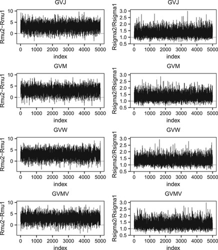
Table 7. Sample sizes of 10 intervals.

Interval	D1Mit156-D1Mit178	D1Mit7-D1Mit46	D1Mit46-D1Mit132	D1Mit132-D1Mit334	D1Mit94-D1Mit218
Total	49	26	26	25	37
$y_1$	17	16	13	11	8
$y_2$	2	2	3	3	8
$y_3$	10	0	2	2	4
$y_4$	20	8	8	9	17
Interval	D1Mit218-D1Mit100	D1Mit14-D1Mit105	D1Mit105-D1Mit159	D1Mit159-D1Mit267	D1Mit267-D1Mit15
Total	37	250	35	35	35
$y_1$	7	137	19	20	15
$y_2$	5	4	0	0	11
$y_3$	4	5	1	6	1
$y_4$	11	104	15	9	8

Similarly, the results for the remaining nine intervals are shown in Tables 8 and 9. The four generalized fiducial methods lead to the same conclusions as the LR method. The QTL effect exists in the D1Mit14–D1Mit105 interval at least with respect to the mean. The D1Mit105–D1Mit159 and D1Mit159–D1Mit267 intervals contain QTLs that affect the variance but not the mean. Note that in the interval D1Mit267–D1Mit15, without the equal-scale assumption, the p-value (0.0673) of the LR method is much smaller than those of the four generalized fiducial methods. When the significance level is 0.1, the LR method declares that a QTL effect exists in the variance but not in the mean. However, as shown in Figure 2, $\{y_{1j},j=1,\dots ,n_1\}$ and $\{y_{4j},j=1,\dots ,n_4\}$ are distributed closely, and the p-value of the F-test for comparing the variances of $\{y_{1j},j=1,\dots ,n_1\}$ and $\{y_{4j},j=1,\dots ,n_4\}$ is 0.3982, much larger than the nominal significance level 0.05. From this perspective, the results of the four generalized p-value methods are more reliable, whereas the LR test method is liberal to some degree.

Figure 2. The boxplot of $\{y_{1j},j=1,\dots ,n_1\}$ and $\{y_{4j},j=1,\dots ,n_4\}$ for D1Mit267-D1Mit15.

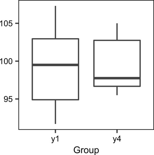
Table 8. Five kinds of p-values in 10 intervals.

Interval	D1Mit156-D1Mit178	D1Mit7-D1Mit46	D1Mit46-D1Mit132	D1Mit132-D1Mit334	D1Mit94-D1Mit218
LR	0.1678	0.3309	0.2524	0.7606	0.3088
GVJ	0.1039	0.2627	0.6578	0.7792	0.3849
GVM	0.1078	0.2847	0.7427	0.7688	0.3996
GVW	0.1033	0.2607	0.6013	0.7554	0.4274
GVMV	0.1009	0.2779	0.6304	0.7604	0.3676
Interval	D1Mit218-D1Mit100	D1Mit14-D1Mit105	D1Mit105-D1Mit159	D1Mit159-D1Mit267	D1Mit267-D1Mit15
LR	0.7951	0.0001	0.0060	0.0088	0.0673
GVJ	0.6339	0	0.0085	0.0081	0.9175
GVM	0.6704	0	0.0104	0.0115	0.8219
GVW	0.6408	0	0.0091	0.0130	0.9872
GVMV	0.6290	0	0.0090	0.0178	0.9407

Table 9. Five kinds of p-values in 10 intervals under ${\sigma }_1={\sigma }_2=\sigma$ assumption.

Interval	D1Mit156-D1Mit178	D1Mit7-D1Mit46	D1Mit46-D1Mit132	D1Mit132-D1Mit334	D1Mit94-D1Mit218
LR	0.1699	0.9728	0.7918	0.4872	0.5442
GVJ	0.1208	0.9596	0.6928	0.4708	0.4100
GVM	0.1272	0.9764	0.7124	0.5216	0.4032
GVW	0.1268	0.9396	0.6988	0.5168	0.4092
GVMV	0.1120	0.9460	0.6796	0.5124	0.3980
Interval	D1Mit218-D1Mit100	D1Mit14-D1Mit105	D1Mit105-D1Mit159	D1Mit159-D1Mit267	D1Mit267-D1Mit15
LR	0.5022	0.0001	0.1267	0.1706	0.1313
GVJ	0.4132	0	0.1476	0.1756	0.5536
GVM	0.4316	0	0.1380	0.1852	0.4140
GVW	0.3772	0	0.1464	0.1732	0.5820
GVMV	0.4228	0	0.1384	0.1784	0.4456

5. Conclusion

In this paper, we propose four generalized fiducial methods to test the existence of QTL effects between two flanking markers. Based on the simulation results, we find that the generalized fiducial methods can control type I errors fairly well even when sample sizes are less than 50. These four generalized fiducial methods have almost the same power as the LR method under a fair comparison, and they are slightly more powerful than the LR method when ${\sigma }_1={\sigma }_2=\sigma$. The four methods can be extended to test the existence of QTL effects with occurring double recombination, where the data from each of the four groups are from a mixture distribution in both location and scale. Meanwhile, more efficient algorithms should be explored, as our two-block algorithm is somewhat time-consuming. We leave these as directions for future research.

Acknowledgments

We are grateful to the Associate Editor and two reviewers for their thorough reading of our manuscript and the constructive comments that lead to significant improvement of our work.

Disclosure statement

No potential conflict of interest was reported by the authors.

Additional information

Funding

This work was supported by the China Scholarship Council [Grant Number 201906140047] and National Natural Science Foundation of China [Grant Numbers 11801210, 11801359 and 11771145].

References

- Agresti, A., & Caffo, B. (2000). Simple and effective confidence intervals for proportions and differences of proportions result from adding two successes and two failures. The American Statistician, 54(4), 280–288. https://doi.org/https://doi.org/10.1080/00031305.2000.10474560
- Agresti, A., & Coull, B. A. (1998). Approximate is better than ‘exact’ for interval estimation of binomial proportions. The American Statistician, 52(2), 119–126. https://doi.org/https://doi.org/10.2307/2685469
- Bebu, I., Luta, G., Mathew, T., & Agan, B. K. (2016). Generalized confidence intervals and fiducial intervals for some epidemiological measures. International Journal of Environmental Research and Public Health, 13(6), 605. https://doi.org/https://doi.org/10.3390/ijerph13060605
- Cai, T. T. (2005). One-sided confidence intervals in discrete distributions. Journal of Statistical Planning and Inference, 131(1), 63–88. https://doi.org/https://doi.org/10.1016/j.jspi.2004.01.005
- Chen, Z., & Chen, H. (2005). On some statistical aspects of the interval mapping for QTL detection. Statistica Sinica, 15(4), 909–925.
- Cui, Y., & Hannig, J. (2019). Nonparametric generalized fiducial inference for survival functions under censoring. Biometrika, 106(3), 501–518. https://doi.org/https://doi.org/10.1093/biomet/asz016
- Efron, B. (1998). RA Fisher in the 21st century. Statistical Science, 13(2), 95–122. https://doi.org/https://doi.org/10.1214/ss/1028905930
- Fisher, R. A. (1930). Inverse probability. In B. J. Green (Ed.), Mathematical Proceedings of the Cambridge Philosophical Society (Vol. 26, pp. 528–535). Cambridge University Press.
- Fisher, R. A. (1932). Statistical Methods for Research Workers (4th ed.). Oliver & Boyd.
- Frühwirth-Schnatter, S. (2006). Finite Mixture and Markov Switching Models. Springer.
- Gelman, A., Stern, H. S., Carlin, J. B., Dunson, D. B., Vehtari, A., & Rubin, D. B. (2014). Bayesian Data Analysis (3rd ed.). Chapman and Hall/CRC.
- Hannig, J. (2009). On generalized fiducial inference. Statistica Sinica, 19(2), 491–544.
- Hannig, J., Iyer, H., Lai, R. C., & Lee, T. C. (2016). Generalized fiducial inference: A review and new results. Journal of the American Statistical Association, 111(515), 1346–1361. https://doi.org/https://doi.org/10.1080/01621459.2016.1165102
- Hannig, J., Iyer, H., & Patterson, P. (2006). Fiducial generalized confidence intervals. Journal of the American Statistical Association, 101(473), 254–269. https://doi.org/https://doi.org/10.1198/016214505000000736
- Huang, N., Parco, A., Mew, T., Magpantay, G., McCouch, S., Guiderdoni, E., Xu, J., Subudhi, P., Angeles, E. R., & Khush, G. S. (1997). RFLP mapping of isozymes, RAPD and QTLs for grain shape, brown planthopper resistance in a doubled haploid rice population. Molecular Breeding, 3(2), 105–113. https://doi.org/https://doi.org/10.1023/A:1009683603862
- Korol, A., Ronin, Y., Tadmor, Y., Bar-Zur, A., Kirzhner, V., & Nevo, E. (1996). Estimating variance effect of QTL: An important prospect to increase the resolution power of interval mapping. Genetical Research, 67(2), 187–194. https://doi.org/https://doi.org/10.1017/S0016672300033632
- Krishnamoorthy, K., & Lee, M. (2010). Inference for functions of parameters in discrete distributions based on fiducial approach: Binomial and Poisson cases. Journal of Statistical Planning and Inference, 140(5), 1182–1192. https://doi.org/https://doi.org/10.1016/j.jspi.2009.11.004
- Lai, R. C., Hannig, J., & Lee, T. C. (2015). Generalized fiducial inference for ultrahigh-dimensional regression. Journal of the American Statistical Association, 110(510), 760–772. https://doi.org/https://doi.org/10.1080/01621459.2014.931237
- Lander, E. S., & Botstein, D. (1989). Mapping mendelian factors underlying quantitative traits using RFLP linkage maps. Genetics, 121(1), 185–199. https://doi.org/https://doi.org/10.1093/genetics/121.1.185
- Li, X., Su, H., & Liang, H. (2018). Fiducial generalized p-values for testing zero-variance components in linear mixed-effects models. Science China Mathematics, 61(7), 1303–1318. https://doi.org/https://doi.org/10.1007/s11425-016-9068-8
- Li, X., Xu, X., & Li, G. (2007). A fiducial argument for generalized p-value. Science in China Series A: Mathematics, 50(7), 957–966. https://doi.org/https://doi.org/10.1007/s11425-007-0067-7
- Li, X., Zhou, X., & Tian, L. (2013). Interval estimation for the mean of lognormal data with excess zeros. Statistics & Probability Letters, 83(11), 2447–2453. https://doi.org/https://doi.org/10.1016/j.spl.2013.07.004
- Liu, G., Li, P., Liu, Y., & Pu, X. (2020). Hypothesis testing for quantitative trait locus effects in both location and scale in genetic backcross studies. Scandinavian Journal of Statistics, 47(4), 1064–1089. https://doi.org/https://doi.org/10.1111/sjos.v47.4
- McLachlan, G., & Peel, D. (2000). Finite Mixture Models. John Wiley & Sons.
- Nkurunziza, S., & Chen, F. (2011). Generalized confidence interval and p-value in location and scale family. Sankhya B, 73(2), 218–240. https://doi.org/https://doi.org/10.1007/s13571-011-0026-8
- Perng, S., & Littell, R. C. (1976). A test of equality of two normal population means and variances. Journal of the American Statistical Association, 71(356), 968–971. https://doi.org/https://doi.org/10.1080/01621459.1976.10480978
- Rebai, A., Goffinet, B., & Mangin, B. (1994). Approximate thresholds of interval mapping tests for QTL detection. Genetics, 138(1), 235–240. https://doi.org/https://doi.org/10.1093/genetics/138.1.235
- Rebai, A., Goffinet, B., & Mangin, B. (1995). Comparing power of different methods for QTL detection. Biometrics, 51(1), 87–99. https://doi.org/https://doi.org/10.2307/2533317
- Schaarschmidt, F., Sill, M., & Hothorn, L. A. (2008). Approximate simultaneous confidence intervals for multiple contrasts of binomial proportions. Biometrical Journal, 50(5), 782–792. https://doi.org/https://doi.org/10.1002/bimj.v50:5
- Sugiyama, F., Churchill, G. A., Higgins, D. C., Johns, C., Makaritsis, K. P., Gavras, H., & Paigen, B. (2001). Concordance of murine quantitative trait loci for salt-induced hypertension with rat and human loci. Genomics, 71(1), 70–77. https://doi.org/https://doi.org/10.1006/geno.2000.6401
- Williams, J. P., & Hannig, J. (2019). Nonpenalized variable selection in high-dimensional linear model settings via generalized fiducial inference. The Annals of Statistics, 47(3), 1723–1753. https://doi.org/https://doi.org/10.1214/18-AOS1733
- Wu, R., Ma, C., & Casella, G. (2007). Statistical Genetics of Quantitative Traits: Linkage, maps and QTL. Springer.
- Wu, W. H., & Hsieh, H. N. (2014). Generalized confidence interval estimation for the mean of delta-lognormal distribution: An application to New Zealand trawl survey data. Journal of Applied Statistics, 41(7), 1471–1485. https://doi.org/https://doi.org/10.1080/02664763.2014.881780
- Xu, X., & Li, G. (2006). Fiducial inference in the pivotal family of distributions. Science in China Series A, 49(3), 410–432. https://doi.org/https://doi.org/10.1007/s11425-006-0410-4
- Zhang, H., Chen, H., & Li, Z. (2008). An explicit representation of the limit of the LRT for interval mapping of quantitative trait loci. Statistics & Probability Letters, 78(3), 207–213. https://doi.org/https://doi.org/10.1016/j.spl.2007.05.020