Optimal model averaging estimator for multinomial logit models

Abstract

In this paper, we study optimal model averaging estimators of regression coefficients in a multinomial logit model, which is commonly used in many scientific fields. A Kullback–Leibler (KL) loss-based weight choice criterion is developed to determine averaging weights. Under some regularity conditions, we prove that the resulting model averaging estimators are asymptotically optimal. When the true model is one of the candidate models, the averaged estimators are consistent. Simulation studies suggest the superiority of the proposed method over commonly used model selection criterions, model averaging methods, as well as some other related methods in terms of the KL loss and mean squared forecast error. Finally, the website phishing data is used to illustrate the proposed method.

Keywords:

• Model averaging
• multinomial logit model
• Kullback–Leibler loss
• asymptotically optimal

1. Introduction

Model selection is a traditional data analysis methodology. By minimizing a model selection criterion, such as Akaike information criterion (AIC) (Akaike, 1973), Bayesian information criterion (BIC) (Schwarz, 1978) and Mallow's C${}_p$ (Mallows, 1973), one model can be chosen from a number of candidate models. After that, one can make statistical inferences under the selected model. In this progress, we ignore the additional uncertainty or even bias introduced by the model selection produce, and thus often underreport the variance of inferences, as discussed in H. Wang et al. (2009). Instead of focusing on one model, the model averaging approach considers a series of candidate models and gives higher weights to the better models. It is an integrated progress that avoids ignoring the uncertainty introduced by the model selection procedure and reduces the risk in regression estimations.

Model averaging can be classified as Bayesian model averaging (BMA) and Frequentist model averaging (FMA). Compared with the FMA approach, there has been an enormous literature about the BMA method, See Hoeting et al. (1999) for a comprehensive review. Unlike the BMA approach which considers the model uncertainty by giving a prior probability to each candidate model, FMA approach does not require priors and the corresponding estimators are totally determined by the data itself. Therefore, the current studies pay more attention to the FMA approach in statistics and econometrics.

In recent years, optimal model averaging methods have received a substantial amount of interests. Hansen (2007) proposed a Mallows model averaging (MMA) method for linear regression models with independent and homoscedastic errors. He developed its asymptotic optimality for a class of nested models by constraining the model weights in a special discrete set. A. T. Wan et al. (2010) provided a more flexible theoretical framework for the MMA which kept its asymptotic optimality for continuous weights and non-nested models. Hansen and Racine (2012), Liu and Okui (2013) developed a jackknife model averaging (JMA) method and heteroscedasticity-robust C${}_p$ model averaging (HRC${}_p$) for the linear regression with independent and heteroscedastic errors, respectively. Zhang et al. (2013) broadened the JMA to the linear regression with dependent errors. Cheng et al. (2015) provided a feasible autocovariance-corrected MMA method to select weights across generalized least squares for the linear regression with time series errors. Zhu et al. (2018) proposed the MMA for multivariate multiple regression models.

Hansen's approach and the subsequent extensions listed above mainly focus on linear models. Recently, some optimal model averaging literatures for nonlinear models have also been developed, including optimal model averaging criterion for partially linear models (Zhang & Wang, 2019), quantile regressions (Lu & Su, 2015), generalized linear models and generalized linear mixed-effects models (Zhang et al., 2016), varying coefficient models (Li et al., 2018), varying-coefficients partially linear models (Zhu et al., 2019), spatial autoregressive models (Zhang & Yu, 2018), and others. All of these methods are asymptotically optimal in the sense of achieving the lowest loss in the large sample case. To the best of our knowledge, there are few optimal averaging estimations for a multinomial logit model that allows all candidate models to be possibly misspecified. The main contribution of this paper is to fill this gap.

The multinomial logit model is widely used in marketing research (Guadagni & Little, 1983), risk analysis (Bayaga, 2010), credit ratings (Ederington, 1985) and other fields including categorical data. A. T. Wan et al. (2014) developed the ‘approximately optimal’ (A-opt) method for the multinomial logit model under a local misspecification model assumption but did not establish asymptotic optimality of the resulting model averaging estimator. Besides, there have been many debates concerning the realism of the local misspecification assumption, e.g., Raftery and Zheng (2003). After that, S. Zhao et al. (2019) proposed M-fold cross-validation (MCV) criterion for the multinomial logit model and yielded forecasting superior to the strategy proposed by A. T. Wan et al. (2014). Then, its asymptotic optimality is proved for the dimension of covariates being fixed.

These two papers for multinomial logit models listed above both concerned a squared estimation error-based risk. Different from squared errors, the KL loss was produced to measure the closeness between the model and the true data generating process. Then, there are amounts of criterion developed from the KL loss, such as Generalised information criteria (GIC) (Konishi & Kitagawa, 1996), Kullback–Leibler information criteria (KIC) (Cavanaugh, 1999) and an improved version of a criterion based on the Akaike information criterion (AIC${}_c$) (Hurvich et al., 1998). In addition, Zhang et al. (2015) clarified that the model averaging methods based on the KL loss yield better forecasts than these model averaging approaches in terms of squared errors under linear regressions. Motivated by these facts, to propose a novel model averaging method based on the KL loss seems to be potentially interesting. Our simulation study demonstrates that the model averaging method based on the KL loss has strong competitive advantages than the model averaging strategy by considering the squared estimation error for the multinomial logit model.

In order to develop an optimal model averaging method for the multinomial logit model, the weights are obtained through minimizing the KL loss. That is, we use a plug-in estimator of the KL loss plus a penalty term as the weight choice criterion, which is equivalent to penalizing the negative log-likelihood. It is interesting to note that this criterion reduces to the Mahalanobis Mallows criterion of Zhu et al. (2018) where they assume that the distribution of multiple responses is multivariate normal. The asymptotic optimality based on the KL loss of the proposed method is built on the consistency of estimators in misspecified models which is more flexible than the above-mentioned local misspecification assumption. Moreover, the asymptotic optimality will be established for the dimension of covariates being either fixed or diverging.

This article is the first study that proposes optimal model averaging estimation for multinomial logit models based on the KL loss. When the number of candidate models is small, the corresponding numerically solutions obtained are nearly instantaneous. If the number of candidate models is large, the computational burden of our model averaging procedure will be heavy. In this case, a model screening step prior to model averaging is desirable. That is, we use penalized regression with LASSO (Friedman et al., 2010) to prepare candidate models. Different tuning parameters may results in different models, which will be included in our resulting candidate models. Using the website phishing data, we demonstrate the superiority of our proposed method.

Our work is related to Zhang et al. (2016), which developed the model averaging method for univariate generalized linear models. We differ from this study by establishing the asymptotic optimality based on some original conditions, while they prove the asymptotic optimality by assuming some conclusions are valid. Moreover, we discuss the case when the true model is one of the candidate models and prove that the model averaging estimators based on our weight choice criterion are consistent.

The remainder of this article is organized as follows. In Section 2, we first describe the multinomial logit model. Then, we introduce the model averaging estimation for the multinomial logit model and propose a weight choice criterion by considering the KL loss. The asymptotic optimality of the proposed method and the estimation consistency are discussed in Sections 3 and 4, respectively. Sections 5 and 6 present the numerical results through various simulations and a real data example, respectively. Technical proofs of the main results are presented in the Appendix.

2. Model framework and weight choice

2.1. Multinomial logit model

Consider a general discrete choice model with n independent individuals and d nominal alternatives. And $y_i=j$ means individual i selects alternative j. We use a multinomial logit regression to describe the discrete choice model (A. T. Wan et al., 2014). The corresponding assumption is that the log odds of category j relative to the reference category (without losing generality, we regard alternative d as reference) are determined by a linear combination of regressors. Thus, the choice probabilities for the ith individual can then be expressed as (1) $\begin{array}{r}\{\begin{array}{l}{\displaystyle f(y_i=j|{\mathit{X}}_i)}\\ =\frac{\exp \left({\mathit{X}}_i{\text{β}}_j\right)}{1+\sum _{j=1}^{d-1}\exp \left({\mathit{X}}_i{\text{β}}_j\right)},\mathrm{f}\mathrm{o}\mathrm{r}j=1,\dots ,(d-1),\\ {\displaystyle f(y_i=d|{\mathit{X}}_i)}\\ =\frac{1}{1+\sum _{j=1}^{d-1}\exp \left({\mathit{X}}_i{\text{β}}_j\right)},\end{array}\end{array}$(1) where $\mathit{X}$ is an $n\times k$ covariate matrix with full column rank, ${\mathit{X}}_i$ is constructed from the ith row of $\mathit{X}$, and ${\text{β}}_j$ is an unknown parameter vector. We first assume k to be fixed and discuss the diverging situation in Section 3. Formula (1(1) $\begin{array}{r}\{\begin{array}{l}{\displaystyle f(y_i=j|{\mathit{X}}_i)}\\ =\frac{\exp \left({\mathit{X}}_i{\text{β}}_j\right)}{1+\sum _{j=1}^{d-1}\exp \left({\mathit{X}}_i{\text{β}}_j\right)},\mathrm{f}\mathrm{o}\mathrm{r}j=1,\dots ,(d-1),\\ {\displaystyle f(y_i=d|{\mathit{X}}_i)}\\ =\frac{1}{1+\sum _{j=1}^{d-1}\exp \left({\mathit{X}}_i{\text{β}}_j\right)},\end{array}\end{array}$(1) ) can be rewritten as an exponential family form. (2) $\begin{array}{r}f(y_i|{\mathit{\theta }}_i,{\mathit{X}}_i)=\exp \left\{T(y_i{)}^{\mathrm{T}}{\mathit{\theta }}_i-b({\mathit{\theta }}_i)\right\},i=1,\dots ,n,\end{array}$(2) where ${\mathit{\theta }}_i=({\theta }_{i1},\dots ,{\theta }_{i(d-1)}{)}^{\mathrm{T}}$ is a parameter vector, with the canonical parameter ${\theta }_{ij}$ connecting the parameters ${\text{β}}_j$ and the k-dimension covariate vector in the form ${\theta }_{ij}={\mathit{X}}_i{\text{β}}_j$. And ${\mathit{\theta }}_i=(I_{d-1}\otimes {\mathit{X}}_i)\text{β}$, where ⊗ is a Kronecker product, $I_{d-1}$ is a $(d-1)\times (d-1)$ identity matrix, and $\text{β}=({\text{β}}_1^{\mathrm{T}},\dots ,{\text{β}}_{d-1}^{\mathrm{T}}{)}^{\mathrm{T}}$, which is a $k(d-1)\times 1$ parameter vector. Besides, $b\left({\mathit{\theta }}_i\right)=\log (\sum _{j=1}^{d-1}\exp \left({\theta }_{ij}\right)+1)$ is a vector-valued function, $T\left(y\right)=({\mathit{I}}_{\{y=1\}},\dots ,{\mathit{I}}_{\{y=d-1\}}{)}^{\mathrm{T}}$, and ${\mathit{I}}_{\{\cdot \}}$ is an indicator function.

2.2. Model averaging estimator

We denote a set of S candidate models $M_1,\dots ,M_S$ by (3) $\begin{array}{rl}& M_s:f\left(y_i|{\mathit{\theta }}_i\right\{{\text{β}}_s\},{\mathit{X}}_{\left(s\right),i})\\ & =\exp \left\{T(y_i{)}^{\mathrm{T}}\right(I_{d-1}\otimes {\mathit{X}}_{\left(s\right),i}){\text{β}}_s\\ & -b\left(\right(I_{d-1}\otimes {\mathit{X}}_{\left(s\right),i}){\text{β}}_s)\phantom{T(y_i{)}^{\mathrm{T}}}\},\end{array}$(3) where S is fixed, and ${\mathit{X}}_{\left(s\right)}$ is an $n\times k_s$ matrix containing $k_s$ columns of $\mathit{X}$ with full column rank, whose rows are ${\mathit{X}}_{\left(s\right),1},\dots ,$ ${\mathit{X}}_{\left(s\right),n}$. Under the sth candidate model, the maximum-likelihood estimator of the regression coefficients is ${\widehat{\text{β}}}_s$. And let ${\widehat{\text{β}}}_s\in R^{(d-1)\times k_s}$ be the subvector containing estimators in ${\widehat{\text{β}}}_{\left(s\right)}\in R^{(d-1)\times k}$. Note that the rest components of ${\widehat{\text{β}}}_{\left(s\right)}$ are restricted to be zeros. Let ${\mathit{\theta }}_{0i}$ be the true value of ${\mathit{\theta }}_i$. And ${\mathit{\theta }}_{0i}$ is not required that there exists a ${\text{β}}_0$ so that ${\mathit{\theta }}_{0i}=(I_{d-1}\otimes {\mathit{X}}_i){\text{β}}_0$. Thus, each of the candidate models can be misspecified. After their maximum-likelihood estimators are obtained, we need to determine the weight of each candidate model. Let $\mathit{\omega }=(w_1,\dots ,w_S)$ be a weight vector in the unit simplex of $R^S:H=\left\{\mathit{\omega }\in [0,1{]}^S,\sum _{s=1}^S{w}_s=1\right\}$. Then the model averaging estimator of $\widehat{\text{β}}\left(\mathit{\omega }\right)$ is $\widehat{\text{β}}\left(\mathit{\omega }\right)=\sum _{s=1}^S{w}_s{\widehat{\text{β}}}_{\left(s\right)}.$

Let $\mathit{Y}=\left(T\right(y_1),\dots ,T(y_n){)}^{\mathrm{T}}$, $\mathit{U}=E\left(\mathit{Y}\right)$ be $n\times (d-1)$ matrices, $\mathbf{\Theta }=({\mathit{\theta }}_1,\dots ,{\mathit{\theta }}_n{)}^{\mathrm{T}}$ be an $n\times (d-1)$ parameter matrix and ${\mathbf{\Theta }}_{\mathbf{0}}=({\mathit{\theta }}_{01},\dots ,{\mathit{\theta }}_{0n}{)}^{\mathrm{T}}$ be the true value of $\mathbf{\Theta }$. We put the model estimator in vector form by using the vectoring operation $\mathrm{Vec}(\cdot )$, which creates a column vector by stacking the column vectors of below one another. Then, the model averaging estimator can be expressed as (4) $\begin{array}{r}\mathrm{Vec}\left({\mathbf{\Theta }}^{\mathrm{T}}\right\{\widehat{\text{β}}\left(\mathit{\omega }\right)\left\}\right)=\mathit{Z}\widehat{\text{β}}\left(\mathit{\omega }\right),\end{array}$(4) where $\mathit{Z}=\left(\right(I_{d-1}\otimes {\mathit{X}}_1{)}^{\mathrm{T}},\dots ,(I_{d-1}\otimes {\mathit{X}}_n{)}^{\mathrm{T}}{)}^{\mathrm{T}}$, which is an $n(d-1)\times k(d-1)$ matrix.

2.3. KL loss-based weight choice criterion

For linear models, the weight choice criterion is based on squared prediction error. In this paper, we use the KL divergence as a replacement for the squared prediction error to establish the asymptotic optimality. The KL loss of $\mathbf{\Theta }\left\{\widehat{\text{β}}\right(\mathit{\omega }\left)\right\}$ is $\begin{array}{rl}KL\left(\mathit{\omega }\right)& =2\sum _{i=1}^n{E}_{{\mathit{Y}}^{\ast }}\{\log \{f\left({\mathit{Y}}^{\ast }|{\mathbf{\Theta }}_0\right)\}\\ & -\log \left(f\right[{\mathit{Y}}^{\ast }|\mathbf{\Theta }\left\{\widehat{\text{β}}\right(\mathit{\omega }\left)\right\}\left]\right)\}\\ & =2B\left\{\widehat{\text{β}}\right(\mathit{\omega }\left)\right\}-2\mathrm{Vec}({\mathit{U}}^{\mathrm{T}}{)}^{\mathrm{T}}\mathrm{Vec}({\mathbf{\Theta }}^{\mathrm{T}}\left\{\widehat{\text{β}}\right(\mathit{\omega }\left)\right\})\\ & -2B_0+2\mathrm{Vec}({\mathit{U}}^{\mathrm{T}}{)}^{\mathrm{T}}\mathrm{Vec}({\mathbf{\Theta }}_0^{\mathrm{T}})\\ & =2J\left(\mathit{\omega }\right)-2B_0+2\mathrm{Vec}({\mathit{U}}^{\mathrm{T}}{)}^{\mathrm{T}}\mathrm{Vec}({\mathbf{\Theta }}_0^{\mathrm{T}}),\end{array}$ where ${\mathit{Y}}^{\ast }=\mathit{U}+{\mathbf{\Xi }}^{\ast }$ is another realization from $f\left({\mathit{Y}}^{\ast }|{\mathbf{\Theta }}_0\right)$, ${\mathbf{\Xi }}^{\ast }$ is independent of $\mathbf{\Xi }$, $\mathbf{\Xi }=\mathit{Y}-\mathit{U}$, $B_0=$ $\sum _{i=1}^{n}b\left({\mathit{\theta }}_{0i}\right)$, $J\left(\mathit{\omega }\right)=B\left\{\widehat{\text{β}}\right(\mathit{\omega }\left)\right\}-\mathrm{Vec}({\mathit{U}}^{\mathrm{T}}{)}^{\mathrm{T}}\mathrm{Vec}{\mathbf{\Theta }}^{\mathrm{T}}\{\widehat{\text{β}}\left(\mathit{\omega }\right)\}$, and $B\left\{\widehat{\text{β}}\right(\mathit{\omega }\left)\right\}=\sum _{i=1}^{n}b\left({\mathit{\theta }}_i\right\{\widehat{\text{β}}\left(\mathit{\omega }\right)\left\}\right)$.

Because of the relationship between $J\left(\mathit{\omega }\right)$ and $KL\left(\mathit{\omega }\right)$, we can obtain $\mathit{\omega }$ to minimize $J\left(\mathit{\omega }\right)$ instead of $KL\left(\mathit{\omega }\right)$. In practice, minimizing $J\left(\mathit{\omega }\right)$ is infeasible because the value of $\mathit{U}$ is unknown. A intuition idea is that we can plug $\mathit{Y}$ into $J\left(\mathit{\omega }\right)$ instead of $\mathit{U}$. That is, we can get $\mathit{\omega }$ by minimizing $J^{\ast }\left(\mathit{\omega }\right)=B\left\{\widehat{\text{β}}\right(\mathit{\omega }\left)\right\}-\mathrm{Vec}({\mathit{Y}}^{\mathrm{T}}{)}^{\mathrm{T}}\mathrm{Vec}({\mathbf{\Theta }}^{\mathrm{T}}\left\{\widehat{\text{β}}\right(\mathit{\omega }\left)\right\})$. But, this progress will lead to overfitting. Motivated by that $J^{\ast }\left(\mathit{\omega }\right)$ equals the corresponding negative log-likelihood of $\mathrm{Vec}\left({\mathbf{\Theta }}^{\mathrm{T}}\right\{\widehat{\text{β}}\left(\mathit{\omega }\right)\left\}\right)=\mathit{Z}\widehat{\text{β}}\left(\mathit{\omega }\right)$. We add a penalty term ${\lambda }_n(d-1){\mathit{\omega }}^{\mathrm{T}}\mathit{K}$ to $2J^{\ast }\left(\mathit{\omega }\right)$, where $\mathit{K}=(k_1,\dots ,k_S{)}^{\mathrm{T}}$, and $k_s$ is the number of columns of $\mathit{X}$ used in the sth candidate model. And the weight choice criterion is introduced as $\begin{array}{rl}\mathrm{\wp }\left(\mathit{\omega }\right)& =2B\left\{\widehat{\text{β}}\right(\mathit{\omega }\left)\right\}-2\mathrm{Vec}({\mathit{Y}}^{\mathrm{T}}{)}^{\mathrm{T}}\mathrm{Vec}({\mathbf{\Theta }}^{\mathrm{T}}\left\{\widehat{\text{β}}\right(\mathit{\omega }\left)\right\})\\ & +{\lambda }_n(d-1){\mathit{\omega }}^{\mathrm{T}}\mathit{K}.\end{array}$ The resultant weight vector is defined as $\hat{\mathit{\omega }}=\arg \underset{\mathit{\omega }\in H}{min}\mathrm{\wp }\left(\mathit{\omega }\right)$. Because $\mathrm{\wp }\left(\mathit{\omega }\right)$ is convex in $\mathit{\omega }$, the global optimization can be performed efficiently through constrained optimization programming. For example, the fmincon of MATLAB can be applied for this purpose. Note that when we restrict one element of $\mathit{\omega }$ to 1 others 0, then $\mathrm{\wp }\left(\mathit{\omega }\right)$ is equivalent to AIC and BIC in the sense of choosing weights when ${\lambda }_n=2$ and ${\lambda }_n=\log \left(n\right)$, respectively. In addition, when ${\lambda }_n=2$, the criterion $\mathrm{\wp }\left(\mathit{\omega }\right)$ can reduce to the Mahalanobis Mallows criterion of Zhu et al. (2018) where they assume that the distribution of multiple responses is multivariate normal.

3. Asymptotic optimality

This section presents the main theoretic results of this paper, which demonstrates the asymptotic optimality of the model averaging estimator $\mathbf{\Theta }\left\{\widehat{\text{β}}\right(\hat{\mathit{\omega }}\left)\right\}$. We define the pseudo true regression parameter vector as ${\text{β}}_{\left(s\right)}^{\ast }$ which minimizes the KL divergence between the true model and the sth candidate model. From Theorem 3.2 of White (1982), when the dimension of ${\text{β}}_{\left(s\right)}^{\ast }$, k, is fixed, under some regularity conditions, we have (5) $\begin{array}{r}\Vert {\widehat{\text{β}}}_{\left(s\right)}-{\text{β}}_{\left(s\right)}^{\ast }\Vert =O_p\left(n^{-1/2}\right).\end{array}$(5) Before we provide the relevant theorems, we first list the relevant notations in this paper. Let ${\text{β}}^{\ast }\left(\mathit{\omega }\right)=\sum _{s=1}^S{w}_s{\text{β}}_{\left(s\right)}^{\ast }$, $K{L}^{\ast }\left(\mathit{\omega }\right)=2B\left\{{\text{β}}^{\ast }\right(\mathit{\omega }\left)\right\}-2\mathrm{Vec}({\mathit{U}}^{\mathrm{T}}{)}^{\mathrm{T}}\mathrm{Vec}({\mathbf{\Theta }}^{\mathrm{T}}\left\{{\text{β}}^{\ast }\right(\mathit{\omega }\left)\right\})-2B_0+2\mathrm{Vec}({\mathit{U}}^{\mathrm{T}}{)}^{\mathrm{T}}\mathrm{Vec}$ $\left({\mathbf{\Theta }}_0^{\mathrm{T}}\right)$, ${\xi }_n=\underset{\mathit{\omega }\in H}{inf}K{L}^{\ast }\left(\mathit{\omega }\right)$, ${\mathbf{\Xi }}_i$ be the ith row of $\mathbf{\Xi }$, $\overline{\lambda }=\underset{i\in \{1,\dots ,n\}}{max}{\lambda }_{max}$ $\{\mathrm{Cov}({\mathbf{\Xi }}_i\left)\right\},$ and $\underset{\_}{\lambda }=\underset{i\in \{1,\dots ,n\}}{min}$ ${\lambda }_{min}\{\mathrm{Cov}({\mathbf{\Xi }}_i\left)\right\}$, where $\mathrm{Cov}(\cdot )$, ${\lambda }_{max}\{\cdot \}$ and ${\lambda }_{min}\{\cdot \}$ denote the covariance, the maximum and minimum eigenvalues of a matrix, respectively. Note that all the limiting properties here and throughout the text hold under $n\to \mathrm{\infty }$. The following conditions will be made:

R.1	There exist constants $\underset{\_}{C}$ and $\overline{C}$, such that $0<\underset{\_}{C}<{\lambda }_{min}\left\{{\mathit{X}}^{\mathrm{T}}\mathit{X}/n\right\}<{\lambda }_{max}\left\{{\mathit{X}}^{\mathrm{T}}\mathit{X}/n\right\}<\overline{C}$.
R.2	$\underset{i\in \{1,\dots ,n\}}{max}\Vert {\mathit{X}}_i{\Vert }^2/n\to 0$, and there exist constants $C_1$ and $C_2$, such that $0<C1<\underset{\_}{\lambda }<\overline{\lambda }<C_2$.
R.3	$n{\xi }_n^{-2}=o\left(1\right)$.
R.4	$n^{-1/2}{\lambda }_n=O\left(1\right)$.

Remark 3.1

Conditions R.1 and R.2 are regular. Condition R.1 is the same as condition C.2 and the second part of condition C.3 of Zhang et al. (2020). The first part of Condition R.2 is the same as the first part of condition C.3 of Zhang et al. (2020). The second part of Condition R.2 assumes the covariance matrix of ${\mathbf{\Xi }}_i$ is positively definite. Condition R.3 requires ${\xi }_n$ grows at a rate no slower than $n^{\frac{1}{2}}$. And both ${\lambda }_n=2$ and ${\lambda }_n=\log \left(n\right)$ satisfy Condition R.4, which means that if one prefers AIC or BIC, this can be achieved by choosing ${\lambda }_n=2$ or ${\lambda }_n=\log \left(n\right)$. Condition R.4 is also used by Theorem 2 of Zhang et al. (2020).

The following theorem illustrates the asymptotic optimality of the model averaging estimators for fixed k situation.

Theorem 3.1

For fixed k, if Equation (5(5) $\begin{array}{r}\Vert {\widehat{\text{β}}}_{\left(s\right)}-{\text{β}}_{\left(s\right)}^{\ast }\Vert =O_p\left(n^{-1/2}\right).\end{array}$(5) ) and the regularity Conditions R.1–R.4 hold. Then $\hat{\mathit{\omega }}$ is asymptotically optimal in the sense that (6) $\begin{array}{r}\frac{KL\left(\stackrel{\mathbf{ˆ}}{\mathit{\omega }}\right)}{\underset{\mathit{\omega }\in H}{inf}KL\left(\mathit{\omega }\right)}\to 1,\end{array}$(6) where the convergence is in probability.

Remark 3.2

Theorem 1 of S. Zhao et al. (2019) is based on the squared loss. The squared loss only concerns on the point distance. Different from them, the KL loss measures the closeness between the model and the true data generating process, which concerns on the full distribution. In addition, from $KL\left(\mathit{\omega }\right)={\int }_{-\mathrm{\infty }}^{+\mathrm{\infty }}f\left(Y^{\ast }|{\mathbf{\Theta }}_0\right)\log \frac{f\left(Y^{\ast }|{\mathbf{\Theta }}_0\right)}{f\left(Y^{\ast }|\mathbf{\Theta }\right\{\widehat{\text{β}}\left(\mathit{\omega }\right)\left\}\right)}{\mathrm{d}}_{Y^{\ast }}$, we know that the KL loss pays more attention to these points with high probability. However, the squared loss considers all points are equally important.

Considering for diverging k, let ${\text{β}}_s^{\ast }\in R^{(d-1)\times k_s}$ be the corresponding subvector of ${\text{β}}_{\left(s\right)}^{\ast }$ and define $\begin{array}{rl}& B_n\left({\text{β}}_s^{\ast }|\delta \right)\\ & =\{{\text{β}}_s\in R^{(d-1)\times k_s}:\Vert \frac{n^{1/2}}{\left\{\right(d-1)k{\}}^{1/2}}\left({\text{β}}_s-{\text{β}}_s^{\ast }\right)\Vert \le \delta \}.\end{array}$ Let $b^{\left(2\right)}=\frac{{\mathrm{\partial }}^{2}b\left(\mathit{x}\right)}{\mathrm{\partial }\mathit{x}\mathrm{\partial }{\mathit{x}}^{\mathrm{T}}}$, ${\mathit{D}}_s=\mathrm{diag}\left\{b^{\left(2\right)}\right[(I_{d-1}\otimes X_{\left(s\right),i}){\text{β}}_{\mathit{s}}]{\}}_{i=1,\dots ,n}$ and ${\mathit{Z}}_{\left(s\right)}=\left(\right(I_{d-1}\otimes X_{\left(s\right),1}{)}^{\mathrm{T}},(I_{d-1}\otimes X_{\left(s\right),2}{)}^{\mathrm{T}},\dots ,(I_{d-1}\otimes X_{\left(s\right),n}{)}^{\mathrm{T}}{)}^{\mathrm{T}}$, which are $n(d-1)\times n(d-1)$ and $n(d-1)\times k_s(d-1)$ matrices, respectively. We list the following conditions required for the case with diverging k.

R.5	There exists a constant $C_3>0$ such that $\sum _{i=1}^n\Vert {\mathit{X}}_i\Vert /\left(k^{1/2}n\right)\le C_3<\mathrm{\infty }$.
R.6	There exists a constant $C_0>0$ such that for any fixed $\delta >0$, any ${\text{β}}_s\in B_n\left({\text{β}}_s^{\ast }|\delta \right)$ and every $s=1,\dots ,S$, the minimum eigenvalue of $\frac{1}{n}{\mathit{Z}}_{\left(s\right)}^{\mathrm{T}}{\mathit{D}}_s{\mathit{Z}}_{\left(s\right)}$ is bound below by $C_0$ for all sufficiently large n.
R.7	$k^{2}n{\xi }_n^{-2}=o\left(1\right)$.

Remark 3.3

Condition R.5 is implied by condition A.1(iii) of Lu and Su (2015). Condition R.6 guarantees that $\Vert {\widehat{\text{β}}}_{\left(s\right)}-{\text{β}}_{\left(s\right)}^{\ast }\Vert =O_p(n^{-1/2}{k}_s^{1/2}$), which is an extension of the first part of condition C.4 of Zhang et al. (2016). Condition R.7 is an extension of Condition R.3 under the diverging k situation. Condition R.7 allows k to increase with n, but restricts its rate. Obviously, as k increases, ${\xi }_n$ decreases. Therefore, the smaller k is easier to satisfy Condition R.7. In practice, we can exclude redundant variables from the candidate set prior to model averaging to control k.

Theorem 3.2

For diverging k, if Conditions R.1–R.2 and R.4–R.7 are satisfied, then (6(6) $\begin{array}{r}\frac{KL\left(\stackrel{\mathbf{ˆ}}{\mathit{\omega }}\right)}{\underset{\mathit{\omega }\in H}{inf}KL\left(\mathit{\omega }\right)}\to 1,\end{array}$(6) ) remains valid as $n\to \mathrm{\infty }$.

Remark 3.4

Note that both ${\lambda }_n=2$ and ${\lambda }_n=\log \left(n\right)$ satisfy Condition R.4. In Section 4, the numerical analysis shows that both of them outperform alternative model selection methods (AIC and BIC) and model averaging methods (Smoothed AIC and Smoothed BIC), respectively. And, when the sample size is small, the optimal value of ${\lambda }_n$ increases as the level of the model misspecification improves.

4. Estimation consistency

Here we would like to comment on the case when the true model is included in the candidate models. That is, $\begin{array}{r}{\mathit{\theta }}_{0i}=(I_{d-1}\otimes {\mathit{X}}_i){\text{β}}_0,\end{array}$ where ${\text{β}}_0\in R^{(d-1)\times k}$ is the true value of $\text{β}$ and the number of non-zero coefficients of ${\text{β}}_0$ is $k_{\mathrm{t}\mathrm{r}\mathrm{u}\mathrm{e}}$. Let ${\mathit{\omega }}_{\mathrm{t}\mathrm{r}\mathrm{u}\mathrm{e}}$ be a weight vector in which the element corresponding to the true model is 1, and all others are 0. When k is fixed, from chapter 3.4.1 of Fahrmeir and Tutz (2013), under some regularity conditions, we have (7) $\begin{array}{r}\Vert \widehat{\text{β}}\left({\mathit{\omega }}_{\mathrm{t}\mathrm{r}\mathrm{u}\mathrm{e}}\right)-{\text{β}}_0\Vert =O_p\left(n^{-1/2}\right).\end{array}$(7) For diverging k, from Theorem 2.1 of Portnoy (1988), under some regularity conditions, we can obtain (8) $\begin{array}{r}\Vert \widehat{\text{β}}\left({\mathit{\omega }}_{\mathrm{t}\mathrm{r}\mathrm{u}\mathrm{e}}\right)-{\text{β}}_0\Vert =O_p\left(k_{\mathrm{t}\mathrm{r}\mathrm{u}\mathrm{e}}^{1/2}{n}^{-1/2}\right).\end{array}$(8) Denote ${\mathit{D}}_i\left(\text{β}\right)=b^{\left(2\right)}\left[\right({\mathit{I}}_{d-1}\otimes {\mathit{X}}_i\left)\text{β}\right]$. In order to prove the estimation consistency, we further impose the following condition.

R.8

There exists $\delta \left(r\right)\ge \underset{\_}{d}>0$, such that uniformly for $\mathit{\omega }\in H$ and $r\in (0,1)$ and for almost all $i\in \{1,\dots ,n\}$, $\begin{array}{rl}& \Vert {\mathit{D}}_i^{1/2}[{\text{β}}_0+r(\widehat{\text{β}}\left(\mathit{\omega }\right)-{\text{β}}_0\left)\right]({\mathit{I}}_{d-1}\otimes {\mathit{X}}_i)\\ & \times {\left(\widehat{\text{β}}\right(\mathit{\omega })-{\text{β}}_0)\Vert }^2/{\Vert \widehat{\text{β}}\left(\mathit{\omega }\right)-{\text{β}}_0\Vert }^2>\delta \left(r\right).\end{array}$

Remark 4.1

Condition R.8 states that most ${\mathit{D}}_i^{1/2}[{\text{β}}_0+r(\widehat{\text{β}}\left(\mathit{\omega }\right)-{\text{β}}_0\left)\right]({\mathit{I}}_{d-1}\otimes {\mathit{X}}_i)\mathrm{s}$ do not degenerate, in the sense that their inner products with $\widehat{\text{β}}\left(\mathit{\omega }\right)-{\text{β}}_0$ do not approach zero, which is implied by ${\lambda }_{min}\{\mathrm{diag}\{{\mathit{D}}_i[{\text{β}}_0+r(\widehat{\text{β}}\left(\mathit{\omega }\right)-{\text{β}}_0\left)\right]{\}}_{i=1,\dots ,n}\}>0$, uniformly for $\mathit{\omega }\in H$ and $r\in (0,1)$, and the first part of condition R.1. Our asymptotic study mainly requires Condition R.8 so that the positive definition of $\mathrm{diag}\left\{{\mathit{D}}_i\right[{\text{β}}_0+r\left(\widehat{\text{β}}\right(\mathit{\omega })-{\text{β}}_0)]{\}}_{i=1,\dots ,n}$ is not necessary.

We now describe the performance of the weighted estimator when the true model is among the candidate models.

Theorem 4.1

When k is fixed and the true model is one of the candidate models, if Conditions R.1, R.2, R.4, R.8 and Equation (7(7) $\begin{array}{r}\Vert \widehat{\text{β}}\left({\mathit{\omega }}_{\mathrm{t}\mathrm{r}\mathrm{u}\mathrm{e}}\right)-{\text{β}}_0\Vert =O_p\left(n^{-1/2}\right).\end{array}$(7) ) are satisfied, then the weighted estimator satisfies (9) $\begin{array}{r}\Vert \widehat{\text{β}}\left(\hat{\mathit{\omega }}\right)-{\text{β}}_0\Vert =O_p\left(n^{-1/2}{\lambda }_n^{1/2}\right)=o_p\left(1\right).\end{array}$(9)

Remark 4.2

Theorem 4.1 states that $\Vert \widehat{\text{β}}\left(\hat{\mathit{\omega }}\right)-{\text{β}}_0\Vert =o_p\left(1\right)$. I conjecture that it may be possible to extend the converge rate of the weighted estimator to $n^{1/2}$, similar to Theorem 2 of Zhang and Liu (2019).

Theorem 4.2

For diverging k, if $k=o\left(n^{1/2}\right)$, Conditions R.1, R.2, R.4, R.8 and Equation (8(8) $\begin{array}{r}\Vert \widehat{\text{β}}\left({\mathit{\omega }}_{\mathrm{t}\mathrm{r}\mathrm{u}\mathrm{e}}\right)-{\text{β}}_0\Vert =O_p\left(k_{\mathrm{t}\mathrm{r}\mathrm{u}\mathrm{e}}^{1/2}{n}^{-1/2}\right).\end{array}$(8) ) are satisfied, then the weighted estimator satisfies (10) $\begin{array}{r}\Vert \widehat{\text{β}}\left(\hat{\mathit{\omega }}\right)-{\text{β}}_0\Vert =O_p\left(k^{1/2}{n}^{-1/2}{\lambda }_n^{1/2}\right)=o_p\left(1\right).\end{array}$(10)

5. Monte Carlo simulations

In this section, we evaluate the empirical performance of our proposed model averaging strategy for the multinomial logit model. We use two versions of our proposed model averaging method named OPT1-KL with ${\lambda }_n=2$ and OPT2-KL with ${\lambda }_n=\log \left(n\right)$ to compare with some alternative FMA methods and model selection strategies. Model selection methods include AIC, BIC, and LASSO proposed by Friedman et al. (2010), where the tuning parameter, $\hat{\zeta }$, is selected by cross-validation. Model averaging strategies include A-OPT (A. T. Wan et al., 2014), MCV (S. Zhao et al., 2019)), Smoothed AIC (SAIC) and Smoothed BIC (SBIC) (Buckland et al., 1997). The SAIC strategy assigns the weight $\begin{array}{r}\exp (-{\mathrm{A}\mathrm{I}\mathrm{C}}_s/2)/\sum _{s=1}^S\exp (-{\mathrm{A}\mathrm{I}\mathrm{C}}_s/2)\end{array}$ to the sth model and SBIC allocates weights similarly.

We use the KL loss for assessment and generate 1000 simulated data. For the convenient comparison, we normalize all KL losses by dividing the KL loss corresponding to the best method. The sample size varies at 100, 200. Note that MCV and A-OPT are the model averaging methods to average estimate of the probability $y_i=j$. Which leads to computing the KL loss is infeasible. Therefore, we compare our methods with MCV and A-OPT in terms of the mean squared forecast error (MSFE) instead of the KL loss. Without loss of generality, we also normalize all MSFEs by dividing the MSFE corresponding to the best method.

Two situations of simulations are used. In the first situation, when the candidate models do not contain the true model, we examine the effect of the changing magnitude of coefficients and the changing level of the model misspecification. Moreover, we consider the case when the number of covariates is diverging with the sample size. Note that all candidate models are misspecified in this situation, so there does not exist the full model. It implies that the A-OPT method is not feasible for this situation. In the second situation, when the candidate models include the true model, we compare our methods with other competitive methods and validate the estimation consistency.

Setting 1. We generate $y_i$ from the setup of the multinomial logit model (2(2) $\begin{array}{r}f(y_i|{\mathit{\theta }}_i,{\mathit{X}}_i)=\exp \left\{T(y_i{)}^{\mathrm{T}}{\mathit{\theta }}_i-b({\mathit{\theta }}_i)\right\},i=1,\dots ,n,\end{array}$(2) ) with the following specifications: $d=3,{\mathit{X}}_{i1}=1$, ${\mathit{X}}_{ij},j=2,\dots ,6$ follow normal distributions with mean zeros, variance ones and the correlation between different components of ${\mathit{X}}_i$ is $\rho =0.75$, and ${\mathit{\theta }}_i=({\theta }_{i1},{\theta }_{i2}{)}^{\mathrm{T}}=(I_2\otimes {\mathit{X}}_i\left)\right({\text{β}}_1^{\mathrm{T}},{\text{β}}_2^{\mathrm{T}}{)}^{\mathrm{T}}$, where $\begin{array}{rl}{\text{β}}_1& ={\gamma }_1(1,1,0.2,-1.2,-0.5,0.7{)}^{\mathrm{T}};\\ {\text{β}}_2& ={\gamma }_1(0.7,0.9,0.3,-1.1,-0.6,0.7{)}^{\mathrm{T}}.\end{array}$ In order to imitate that all candidate models are misspecified, we pretend the last covariate missed. Let ${\mathit{X}}_{i1}$ contain in all candidate models. So there are $2^4-1=15$ candidate models to combine. The parameter ${\gamma }_1$ is used to control the magnitude of coefficients, and we let it vary in the set $\{0.5,1,2\}$.

Simulation results are shown in Table 1. One remarkable aspect of the results is that OPT1-KL and OPT2-KL yield smaller mean and standard deviance (SD) values than the other four competitions (SAIC, SBIC, AIC and BIC) in different magnitudes of coefficients. In the majority of cases, FMA approaches are superior to model selection methods. This pattern appears to be more obvious when ${\gamma }_1$ is small than when it is large. For example, when ${\gamma }_1$ = 0.5, all model averaging methods deliver smaller mean values than model selection strategies. When ${\gamma }_1$ increases to 2, for n = 200, AIC has marginal advantages than SBIC regarding the mean values. This result is reasonable, because when ${\gamma }_1$ is small, and the non-zero coefficients in the true model are all close to zero, which makes it difficult to distinguish the non-zero coefficients from a false model that contains many zeros. As a result, model selection criterion scores can be quite similar for different candidate models and the choice of models becomes unstable. On the other hand, when the absolute values of the non-zero coefficients are large, and a model selection criterion can identify a non-zero coefficient more readily.

Table 1. Simulations results of the KL loss for setting 1.

${\gamma }_1$	n		OPT1-KL	OPT2-KL	SAIC	SBIC	AIC	BIC
0.5	100	Mean	1.2854	1.0000	2.6779	2.2431	3.8806	3.0228
		SD	2.1785	1.0000	5.2774	4.5048	4.5793	4.5313
	200	Mean	1.0181	1.0000	1.8427	1.7991	2.4709	2.2732
		SD	1.6082	1.0000	3.3939	3.0055	2.9032	2.8244
1	100	Mean	1.0359	1.0000	1.9150	1.8519	2.4402	2.3318
		SD	1.5007	1.0000	3.0423	2.7406	2.7229	2.5896
	200	Mean	1.0000	1.0373	1.5212	1.6712	1.8182	1.9670
		SD	1.1837	1.0000	2.2872	2.3921	2.3530	2.4111
2	100	Mean	1.0260	1.0000	1.7058	1.7868	1.9758	2.0719
		SD	1.3210	1.0000	2.6279	2.6401	2.7112	2.6516
	200	Mean	1.0000	1.0173	1.3756	1.5121	1.5009	1.6475
		SD	1.1638	1.0000	2.3457	2.8700	2.6478	3.2289

In addition, we calculate the means of $KL\left(\stackrel{\mathbf{ˆ}}{\mathit{\omega }}\right)/{\mathrm{i}\mathrm{n}\mathrm{f}}_{\mathit{\omega }\in H}KL\left(\mathit{\omega }\right)\left(\mathrm{r}\mathrm{a}\mathrm{t}\mathrm{i}\mathrm{o}\right)$ by methods of OPT1-KL and OPT2-KL with ${\gamma }_1=1$. The values of mean, presented in Figure 1, decrease and approach to 1 as the sample size n increases. This feature verifies asymptotic optimality numerically. Then, we compare our strategy with MCV in terms of MSFE. We generate 100 observations as the training sample and 10 observations as the test sample under setting 1 with ${\gamma }_1=1$. And the simulation results are based on 1000 replications. $\begin{array}{r}\mathrm{M}\mathrm{S}\mathrm{F}\mathrm{E}=\frac{1}{10000}\sum _{r=1}^{1000}\sum _{v=1}^{10}\sum _{j=1}^3({\hat{p}}_{vj}^{\left[r\right]}-p_{vj}^{\left[r\right]}{)}^2,\end{array}$ where ${\hat{p}}_{vj}^{\left[r\right]}$ is the forecast of $p_{vj}^{\left[r\right]}$, which represents the probability that the vth test observation selects alternative j for the rth replication.

Figure 1. The means of ratio by methods of OPT1-KL and OPT2-KL with ${\gamma }_1=1$.

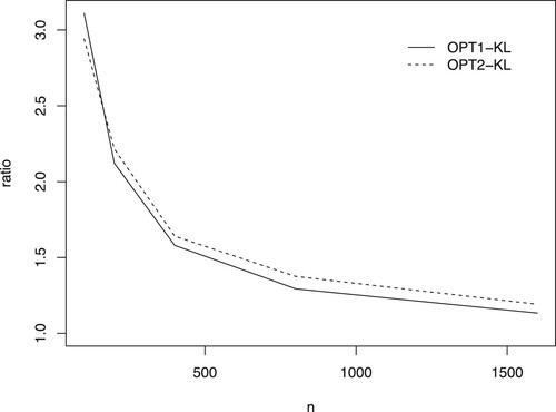
Table 2 shows that our proposed approaches outperform other strategies. Then, SAIC and SBIC perform better than MCV. Note that MCV is the model averaging method based on the squared loss, and our strategy is based on the KL loss. It implies that the approach based on the KL loss has a strong competitive advantage than this approach based on the square loss for a multinomial logit model.

Table 2. Simulation results of MSFE.

		OPT1-KL	OPT2-KL	SAIC	SBIC	AIC	BIC	MCV
	Mean	1.0000	1.0195	1.0703	1.0728	1.2243	1.2424	1.1675
	SD	1.0858	1.0906	1.1869	1.1656	1.3430	1.2729	1.0000

Setting 2. In order to examine the effects of the changing level of the model misspecification, we set ${\theta }_{i1}={\mathit{U}}_i{\text{β}}_1+{\gamma }_2\exp \left(0.5X_{i6}\right)$, ${\theta }_{i2}={\mathit{U}}_i{\text{β}}_2+{\gamma }_2\exp \left(0.6X_{i6}\right)$, and $\begin{array}{rl}{\text{β}}_1& =(1,1,0.2,-1.2,-0.5{)}^{\mathrm{T}};\\ {\text{β}}_2& =(0.7,0.9,0.3,-1.1,-0.6{)}^{\mathrm{T}},\end{array}$ where ${\mathit{U}}_i=(1,X_{i2},\dots ,X_{i5})$, $X_{i2},\dots ,X_{i6}$ have the same specification as the previous design, ${\gamma }_2$ controls the level of the model misspecification, we study it in the set $\{0.25,0.5,0.75\}$. We take the multinomial logit model (3(3) $\begin{array}{rl}& M_s:f\left(y_i|{\mathit{\theta }}_i\right\{{\text{β}}_s\},{\mathit{X}}_{\left(s\right),i})\\ & =\exp \left\{T(y_i{)}^{\mathrm{T}}\right(I_{d-1}\otimes {\mathit{X}}_{\left(s\right),i}){\text{β}}_s\\ & -b\left(\right(I_{d-1}\otimes {\mathit{X}}_{\left(s\right),i}){\text{β}}_s)\phantom{T(y_i{)}^{\mathrm{T}}}\},\end{array}$(3) ) to fit the data. We still omit the last covariate $X_{i6}$ and consider $S=2^4-1$ candidate models.

The simulation results under different levels of the model misspecification are shown in Table 3. It is seen that OPT1-KL and OPT2-KL always deliver better performances than their competitors SAIC/AIC and SBIC/BIC in terms of mean values, respectively. Focusing on SD values, OPT1-KL always performs much better than SAIC and AIC, and OPT2-KL outperforms SBIC and BIC in most cases. It demonstrates the superiority of our methods.

Table 3. Simulations results of the KL loss for setting 2.

${\gamma }_2$	n		OPT1-KL	OPT2-KL	SAIC	SBIC	AIC	BIC
0.25	100	Mean	1.0000	1.0302	1.0886	1.0955	1.3113	1.2951
		SD	1.1114	1.0000	1.2915	1.0422	1.4790	1.1611
	200	Mean	1.0000	1.1340	1.1028	1.2919	1.2384	1.4722
		SD	1.0000	1.0499	1.1158	1.0986	1.2548	1.2265
0.50	100	Mean	1.0000	1.0189	1.0736	1.0566	1.2941	1.2694
		SD	1.1225	1.0000	1.3122	1.0794	1.4152	1.1858
	200	Mean	1.0000	1.1282	1.1018	1.2484	1.2400	1.4465
		SD	1.0000	1.0259	1.1005	1.0071	1.2501	1.1436
0.75	100	Mean	1.0084	1.0000	1.0614	1.0103	1.2938	1.2220
		SD	1.1939	1.0000	1.3298	1.0451	1.6517	1.1342
	200	Mean	1.0000	1.1333	1.0764	1.2175	1.2037	1.4217
		SD	1.0324	1.0108	1.1369	1.0000	1.3275	1.1295

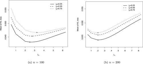
In addition, we explore our strategies with other values of ${\lambda }_n$ differing from 2 and $\log \left(n\right)$. That is, we vary ${\lambda }_n$ from 0.5 to $n^{0.4}$. The simulation results are presented in Figure 2. For cases of ${\gamma }_2=0.25,0.5$ and 0.75, when n = 100, the means of KL loss are minimized at ${\lambda }_n=2.5$, ${\lambda }_n=2.75$ and ${\lambda }_n=3.25$, respectively. It states that when the level of the model misspecification improves, the optimal value of ${\lambda }_n$ increases slightly for the small sample size. For a larger sample size n = 200, the optimal values of ${\lambda }_n$ are same for all cases with ${\lambda }_n=2$.

Figure 2. The relationship between the mean of KL loss and ${\lambda }_n$. The points with the smallest losses are indicated by the filled circle •. (a) n = 100 and (b) n = 200.

Setting 3. This setup discusses the case when the number of covariates is diverging. The data generate progress is the same as those in setting 1. Except that we adapt the covariance matrix to $R=\left(r_{ij}\right)$ with $r_{ij}={0.40}^{|i-j|}$, for that the model screening method is not suitable for the case when the covariances have strong dependence which is implied by the first part of Lemma 3.2 in Ando and Li (2014). Then, ${\text{β}}_1$ and ${\text{β}}_2$ are chosen according to the following cases: $\begin{array}{rl}{\text{β}}_1& =(1,1.2,0,0,1.5,0,0,1.1,0,0,0.1,\\ & \dots ,0.1,0.9{)}_{\left[3n^{1/3}\right]\times 1}^{\mathrm{T}};\\ {\text{β}}_2& =(1,1.3,0,0,2,0,0,1.2,0,0,0.1,\\ & \dots ,0.1,0.8{)}_{\left[3n^{1/3}\right]\times 1}^{\mathrm{T}}.\end{array}$ Similar to setting 1, we also pretend the last covariate was missed. Then, there are $2^{\left[3n^{1/3}\right]-2}-1$ candidate models. The computation burden will be heavy. Therefore, a screening method to screen candidate models is desirable. That is, we use penalized regression with LASSO (Friedman et al., 2010) to prepare candidate models. Different tuning parameters may result in different models, which will be included in our resulting candidate models. Obviously, the resulting candidate model contains lots of redundant variables when the tuning parameter is very small. In order to avoid the generated candidate models including a lot of redundant variables, we use tuning parameters larger than $\hat{\zeta }$ to prepare candidate models.

Simulation results are provided in Table 4. Focusing on the mean values, Table 4 shows that OPT1-KL always performs better than SAIC and AIC, and OPT2-KL still outperforms SBIC and BIC, respectively. In addition, OPT2-KL always outperforms LASSO. It implies the advantages of our proposed method comparing with other competitive methods.

Table 4. Simulations results of the KL loss for setting 3.

n		OPT1-KL	OPT2-KL	SAIC	SBIC	AIC	BIC	LASSO
100	Mean	1.0863	1.0000	1.3113	1.1209	1.4165	1.2136	1.0172
	SD	1.7691	1.3568	2.7897	1.6756	3.1682	1.9177	1.0000
200	Mean	1.0322	1.0000	1.1918	1.0406	1.2664	1.0821	1.1053
	SD	1.1986	1.1635	1.7025	1.4451	1.8834	1.5681	1.0000

Setting 4. This setup verifies the estimation consistency. The data generate progress is the same as those in setting 3. Except that we choose ${\text{β}}_1$ and ${\text{β}}_2$ as follows: $\begin{array}{rl}\mathrm{c}\mathrm{a}\mathrm{s}\mathrm{e}1:{\text{β}}_1& =(1,1.5,3,0,0{)}^{\mathrm{T}};\\ {\text{β}}_2& =(1,1.7,4,0,0{)}^{\mathrm{T}};\end{array}$ and $\begin{array}{rl}\mathrm{c}\mathrm{a}\mathrm{s}\mathrm{e}2:{\text{β}}_1& =(1,1.5,3,1.2,0{)}^{\mathrm{T}};\\ {\text{β}}_2& =(1,1.7,4,1.3,0{)}^{\mathrm{T}}.\end{array}$ All candidate models include $X_{i1}$. Thus, we consider a total of $2^4-1=15$ candidate models. Note that the true model is included in the candidate models. We compare our proposed method with other competitive methods based on the KL loss and MSFE. The results are presented in Tables 5 and 6, respectively. These results show that OPT2-KL always obtain the smallest KL loss and MSFE among these methods, which validates the superiority of our method.

Table 5. Simulations results of the KL loss for setting 4.

Case	n		OPT1-KL	OPT2-KL	SAIC	SBIC	AIC	BIC
1	100	Mean	1.2060	1.0000	1.4672	1.1862	1.2667	1.2462
		SD	1.5345	1.1268	2.1304	1.4188	1.4251	1.0000
	200	Mean	1.1020	1.0000	1.2307	1.0853	1.0256	1.1022
		SD	1.2962	1.0000	1.7283	1.3664	1.0145	1.1259
2	100	Mean	1.1659	1.0000	1.5795	1.3179	1.3301	1.3501
		SD	1.7378	1.0000	2.9602	1.9637	1.8268	1.4928
	200	Mean	1.0311	1.0000	1.2623	1.2498	1.0708	1.3389
		SD	1.5307	1.1471	2.0867	1.6240	1.0798	1.0000

Table 6. Simulations results of MSFE for setting 4.

Case		OPT1-KL	OPT2-KL	SAIC	SBIC	AIC	BIC	A-OPT	MCV
1	Mean	1.0901	1.0000	1.2252	1.1081	1.2523	1.2838	2.0084	1.0225
	SD	1.1847	1.0764	1.3439	1.1847	1.4777	1.4331	14.1238	1.0000
2	Mean	1.0694	1.0000	1.2367	1.1510	1.4000	1.4735	1.8465	1.0653
	SD	1.1278	1.0278	1.2833	1.1722	1.4611	1.5611	10.6498	1.0000

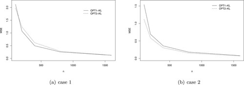
Also, we calculate the mean squared error (MSE) by methods of OPT1-KL and OPT2-KL. $\begin{array}{r}\mathrm{M}\mathrm{S}\mathrm{E}=\frac{1}{1000}\sum _{r=1}^{1000}\Vert {\text{β}}^{\left(r\right)}\left(\hat{\mathit{\omega }}\right)-\text{β}{\Vert }^2,\end{array}$ where ${\text{β}}^{\left(r\right)}\left(\hat{\mathit{\omega }}\right)$ represents the estimator of $\text{β}$ for the rth replication and $\text{β}=({\text{β}}_1^{\mathrm{T}},{\text{β}}_2^{\mathrm{T}}{)}^{\mathrm{T}}$. The MSE curves, shown in Figure 3, decrease and approach zero with the increase of sample size n. The feature confirms estimation consistency numerically.

Figure 3. Assessing the estimation consistency of OPT1-KL and OPT2-KL. (a) case 1 and (b) case 2.

6. An empirical application

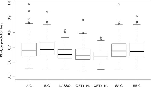
In this part, we apply the proposed method to the website phishing data, which was previously used by Abdelhamid et al. (2014). This data set contains three types of website (702 phishing websites, 548 legitimate websites and 103 suspicious websites). The dependent variables consist of Server Form Handler, Using Pop-Up Window, Fake HTTPs protocol, Request URL, URL of Anchor, Website Traffic, URL Length, Age of Domain and Having IP address. These variables are categorical (or binary). We transform this information into indicator variables. After this operation, the total number of predictors is 16. After the screening method, we analyse this dataset using candidate multinomial logit models. We randomly select 677 observations as the training sample and predict the remaining instances. We repeat this progress 500 times. We use the following KL-type prediction loss $L_{\mathrm{K}\mathrm{L}}$ to measure the prediction performance. $\begin{array}{r}{L}_{\mathrm{K}\mathrm{L}}=-\frac{2}{n_0}\sum _{v=1}^{n_0}\sum _{j=1}^d{I}_{\{y_{\mathrm{t}\mathrm{e}\mathrm{s}\mathrm{t},v}=j\}}\log \left\{\hat{p}\right(y_{\mathrm{t}\mathrm{e}\mathrm{s}\mathrm{t},v}=j\left)\right\},\end{array}$ where $\{y_{\mathrm{t}\mathrm{e}\mathrm{s}\mathrm{t},1},\dots ,y_{\mathrm{t}\mathrm{e}\mathrm{s}\mathrm{t},n_0}\}$ are testing observations, and $\hat{p}(y_{\mathrm{t}\mathrm{e}\mathrm{s}\mathrm{t},v}=j)$ is the predicted probability of the vth test observation taking on j.

Figure 4 shows the box plot of all KL-type prediction losses by seven methods. It is observed that our proposed methods of OPT1-KL and OPT2-KL produce better performances than their competitions SAIC/AIC and SBIC/BIC, respectively. In addition, OPT2-KL outperforms LASSO in terms of the KL loss.

Figure 4. Boxplots of KL-type prediction losses by seven methods in the website phishing data.

In addition, we evaluate the prediction performance based on the hit-rate, which is computed by dividing the number of correct predictions by the size of the test sample. The prediction value of an observation is $j(1\le j\le 3)$ if the predicted probability of this observation taking on j has the largest value among the three predicted probability values. In addition, we also calculate the optimal rate (OPR) and the worst rate (WOR) of each method, which is the proportion of times with the largest hite-rate and the smallest hit-rate. Table 7 presents mean values of hit-rate (HRV), OPR and WOR corresponding to these methods, which shows that OPT1-KL and OPT2-KL methods obtain the larger HRV, OPR and smaller WOR than other competitions SAIC, SBIC, AIC, BIC and LASSO, demonstrating the superiority of our proposed strategies.

Table 7. Out-of-sample performances in the website phishing data.

	OPT1-KL	OPT2-KL	SAIC	SBIC	AIC	BIC	LASSO
HRV	0.8879	0.8921	0.8811	0.8812	0.8799	0.8800	0.8841
OPR	0.2200	0.6100	0.0200	0.0400	0.0100	0.0100	0.0900
WOR	0.0200	0.0200	0.2100	0.2600	0.2600	0.1600	0.0700

Table 8 reports the Diebold–Mariano test (Diebold & Mariano, 2002) results for the differences in hit-rate. Note that a positive Diebold–Mariano statistic indicates that the estimator in the numerator produces a larger hit-rate than the estimator in the denominator. The test statistics and p-values show that the differences in hit-rate between our methods and other strategies are all statistically significant.

Table 8. Diebold–Mariano statistics of hit-rate in the website phishing data.

	$\frac{\mathrm{O}\mathrm{P}\mathrm{T}1-\mathrm{K}\mathrm{L}}{\mathrm{O}\mathrm{P}\mathrm{T}2-\mathrm{K}\mathrm{L}}$	$\frac{\mathrm{O}\mathrm{P}\mathrm{T}1-\mathrm{K}\mathrm{L}}{\mathrm{S}\mathrm{A}\mathrm{I}\mathrm{C}}$	$\frac{\mathrm{O}\mathrm{P}\mathrm{T}1-\mathrm{K}\mathrm{L}}{\mathrm{S}\mathrm{B}\mathrm{I}\mathrm{C}}$	$\frac{\mathrm{O}\mathrm{P}\mathrm{T}1-\mathrm{K}\mathrm{L}}{\mathrm{A}\mathrm{I}\mathrm{C}}$	$\frac{\mathrm{O}\mathrm{P}\mathrm{T}1-\mathrm{K}\mathrm{L}}{\mathrm{B}\mathrm{I}\mathrm{C}}$	$\frac{\mathrm{O}\mathrm{P}\mathrm{T}1-\mathrm{K}\mathrm{L}}{\mathrm{L}\mathrm{A}\mathrm{S}\mathrm{S}\mathrm{O}}$	$\frac{\mathrm{O}\mathrm{P}\mathrm{T}2-\mathrm{K}\mathrm{L}}{\mathrm{S}\mathrm{A}\mathrm{I}\mathrm{C}}$
DM	−7.6502	16.6320	9.7040	14.0080	13.1790	4.9572	16.8250
p-value	0.0000	0.0000	0.0000	0.0000	0.0000	0.0000	0.0000
	$\frac{\mathrm{O}\mathrm{P}\mathrm{T}2-\mathrm{K}\mathrm{L}}{\mathrm{S}\mathrm{B}\mathrm{I}\mathrm{C}}$	$\frac{\mathrm{O}\mathrm{P}\mathrm{T}2-\mathrm{K}\mathrm{L}}{\mathrm{A}\mathrm{I}\mathrm{C}}$	$\frac{\mathrm{O}\mathrm{P}\mathrm{T}2-\mathrm{K}\mathrm{L}}{\mathrm{B}\mathrm{I}\mathrm{C}}$	$\frac{\mathrm{O}\mathrm{P}\mathrm{T}2-\mathrm{K}\mathrm{L}}{\mathrm{L}\mathrm{A}\mathrm{S}\mathrm{S}\mathrm{O}}$	$\frac{\mathrm{S}\mathrm{A}\mathrm{I}\mathrm{C}}{\mathrm{S}\mathrm{B}\mathrm{I}\mathrm{C}}$	$\frac{\mathrm{S}\mathrm{A}\mathrm{I}\mathrm{C}}{\mathrm{A}\mathrm{I}\mathrm{C}}$	$\frac{\mathrm{S}\mathrm{A}\mathrm{I}\mathrm{C}}{\mathrm{B}\mathrm{I}\mathrm{C}}$
DM	22.0980	14.1900	16.1360	8.4057	−0.0124	5.7799	4.1535
p-value	0.0000	0.0000	0.0000	0.0000	0.9901	0.0000	0.0000
	$\frac{\mathrm{S}\mathrm{A}\mathrm{I}\mathrm{C}}{\mathrm{L}\mathrm{A}\mathrm{S}\mathrm{S}\mathrm{O}}$	$\frac{\mathrm{S}\mathrm{B}\mathrm{I}\mathrm{C}}{\mathrm{A}\mathrm{I}\mathrm{C}}$	$\frac{\mathrm{S}\mathrm{B}\mathrm{I}\mathrm{C}}{\mathrm{B}\mathrm{I}\mathrm{C}}$	$\frac{\mathrm{S}\mathrm{B}\mathrm{I}\mathrm{C}}{\mathrm{L}\mathrm{A}\mathrm{S}\mathrm{S}\mathrm{O}}$	$\frac{\mathrm{A}\mathrm{I}\mathrm{C}}{\mathrm{B}\mathrm{I}\mathrm{C}}$	$\frac{\mathrm{A}\mathrm{I}\mathrm{C}}{\mathrm{L}\mathrm{A}\mathrm{S}\mathrm{S}\mathrm{O}}$	$\frac{\mathrm{B}\mathrm{I}\mathrm{C}}{\mathrm{L}\mathrm{A}\mathrm{S}\mathrm{S}\mathrm{O}}$
DM	−5.0119	1.9948	4.0979	−4.7816	−0.0955	−5.7478	−6.4553
p-value	0.0000	0.0474	0.0000	0.0000	0.9240	0.0000	0.0000

7. Discussion

In the context of multinomial logit model, we proposed model averaging estimator and weight choice criterion based on KL loss with a penalty term. And we proved the asymptotic optimality of the resulting model averaging estimator under some regularity conditions. When the true model is one of the candidate models, the averaged estimators are consistent. Also, in order to reduce the computational burden, we applied a model screening step before averaging. Numerical experiments were performed to demonstrate the superiority of the proposed methods over other commonly used model selection strategies, model averaging methods, MCV, Lasso in terms of KL loss and MSFE.

While we consider the multinomial logit model, the extension to other models, such as ordered logit model, warrants further investigation. And the data structure of the regressors further complicates this issue. Another interesting question is how to choose an optimal ${\lambda }_n$. Shen et al. (2004) have proposed an adaptive method to choose ${\lambda }_n$ for model selection criterion in generalized linear models. Building similar methods for our proposed model averaging method to choose an optimal ${\lambda }_n$ warrants future researches.

Disclosure statement

No potential conflict of interest was reported by the author(s).

Correction Statement

This article has been republished with minor changes. These changes do not impact the academic content of the article.

Additional information

Funding

The research is supported by Natural Science Foundation of China (No. 11771268) and a center named Shanghai Research Center for Data Science and Decision Technology.

Appendix

Proof

Proof of Theorem 3.1

Let $\tilde{\mathrm{\wp }}\left(\mathit{\omega }\right)=\mathrm{\wp }\left(\mathit{\omega }\right)-2B_0+2\mathrm{Vec}({\mathit{U}}^{\mathrm{T}}{)}^{\mathrm{T}}\mathrm{Vec}({\mathbf{\Theta }}_0^{\mathrm{T}})$. It's obvious that $\tilde{\mathrm{\wp }}$ and ℘ are equivalent in the sense of choosing weights. From the proof of Theorem 1 in Zhang et al. (2016), Theorem 3.1 is valid if the following holds: (A1) $\begin{array}{r}\underset{\mathit{\omega }\in H}{sup}\frac{|KL\left(\mathit{\omega }\right)-K{L}^{\ast }\left(\mathit{\omega }\right)|}{K{L}^{\ast }\left(\mathit{\omega }\right)}\to o_p\left(1\right)\end{array}$(A1) and (A2) $\begin{array}{r}\underset{\mathit{\omega }\in H}{sup}\frac{|\tilde{\mathrm{\wp }}\left(\mathit{\omega }\right)-K{L}^{\ast }\left(\mathit{\omega }\right)|}{K{L}^{\ast }\left(\mathit{\omega }\right)}\to o_p\left(1\right).\end{array}$(A2) By Equation (5(5) $\begin{array}{r}\Vert {\widehat{\text{β}}}_{\left(s\right)}-{\text{β}}_{\left(s\right)}^{\ast }\Vert =O_p\left(n^{-1/2}\right).\end{array}$(5) ), we can know that uniformly for $\mathit{\omega }\in H$ (A3) $\begin{array}{r}\Vert \widehat{\text{β}}\left(\mathit{\omega }\right)-{\text{β}}^{\ast }\left(\mathit{\omega }\right)\Vert =\Vert \sum _{s=1}^S{\omega }_s({\widehat{\text{β}}}_{\left(s\right)}-{\text{β}}_{\left(s\right)}^{\ast })\Vert =O_p\left(n^{-1/2}\right).\end{array}$(A3) From (A3(A3) $\begin{array}{r}\Vert \widehat{\text{β}}\left(\mathit{\omega }\right)-{\text{β}}^{\ast }\left(\mathit{\omega }\right)\Vert =\Vert \sum _{s=1}^S{\omega }_s({\widehat{\text{β}}}_{\left(s\right)}-{\text{β}}_{\left(s\right)}^{\ast })\Vert =O_p\left(n^{-1/2}\right).\end{array}$(A3) ), ${\lambda }_{max}\left({\mathit{Z}}^{\mathrm{T}}\mathit{Z}\right)={\lambda }_{max}\left({\mathit{X}}^{\mathrm{T}}\mathit{X}\right)$, Condition R.1 and Taylor expansion uniformly for $\mathit{\omega }\in H$ (A4) $\begin{array}{rl}& \left|B\right\{\widehat{\text{β}}\left(\mathit{\omega }\right)\}-B\left\{{\text{β}}^{\ast }\left(\mathit{\omega }\right)\right\}|\\ & =|\sum _{i=1}^n[(\frac{\exp \left({\mathit{X}}_{\mathit{i}}\widetilde{\text{β}}\right(\mathit{\omega }{)}_1){\mathit{X}}_i}{\sum _{j=1}^{d-1}(\exp ({\mathit{X}}_{\mathit{i}}\widetilde{\text{β}}\left(\mathit{\omega }{)}_j\right)+1},\\ & \dots ,\frac{\exp \left({\mathit{X}}_{\mathit{i}}\widetilde{\text{β}}\right(\mathit{\omega }{)}_{d-1}){\mathit{X}}_i}{\sum _{j=1}^{d-1}(\exp ({\mathit{X}}_{\mathit{i}}\widetilde{\text{β}}\left(\mathit{\omega }{)}_j\right)+1})\left(\widehat{\text{β}}\right(\mathit{\omega })-{\text{β}}^{\ast }(\mathit{\omega }\left)\right)]|\\ & \le \Vert \widehat{\text{β}}\left(\mathit{\omega }\right)-{\text{β}}^{\ast }\left(\mathit{\omega }\right)\Vert \sum _{i=1}^n\Vert (\frac{\exp \left({\mathit{X}}_{\mathit{i}}\widetilde{\text{β}}\right(\mathit{\omega }{)}_1){\mathit{X}}_i}{\sum _{j=1}^{d-1}(\exp ({\mathit{X}}_{\mathit{i}}\widetilde{\text{β}}\left(\mathit{\omega }{)}_j\right)+1}\\ & \times ,\dots ,\frac{\exp \left({\mathit{X}}_{\mathit{i}}\widetilde{\text{β}}\right(\mathit{\omega }{)}_1){\mathit{X}}_i}{\sum _{j=1}^{d-1}(\exp ({\mathit{X}}_{\mathit{i}}\widetilde{\text{β}}\left(\mathit{\omega }{)}_j\right)+1)})\Vert \\ & \le \Vert \widehat{\text{β}}\left(\mathit{\omega }\right)-{\text{β}}^{\ast }(\mathit{\omega }\Vert \sum _{l=1}^{n(d-1)}\Vert {\mathit{Z}}_l\Vert \\ & \le \Vert \widehat{\text{β}}\left(\mathit{\omega }\right)-{\text{β}}^{\ast }(\mathit{\omega }\Vert \sum _{l=1}^{n(d-1)}(1+\Vert {\mathit{Z}}_l{\Vert }^2)\\ & =\Vert \widehat{\text{β}}\left(\mathit{\omega }\right)-{\text{β}}^{\ast }(\mathit{\omega }\Vert [\mathrm{trace}\left({\mathit{Z}}^{\mathrm{T}}\mathit{Z}\right)+n(d-1)]\\ & \le \Vert \widehat{\text{β}}\left(\mathit{\omega }\right)-{\text{β}}^{\ast }(\mathit{\omega }\Vert [{\lambda }_{max}\left({\mathit{Z}}^{\mathrm{T}}\mathit{Z}\right)\left(k\right(d-1\left)\right)+n(d-1)]\\ & =O_p\left(n^{1/2}\right),\end{array}$(A4) where $\widetilde{\text{β}}\left(\mathit{\omega }\right)$ is between $\widehat{\text{β}}\left(\mathit{\omega }\right)$ and ${\text{β}}^{\ast }\left(\mathit{\omega }\right)$. From ${\mathit{U}}_{ij}<1,i=1,\dots ,n,j=1,\dots ,(d-1)$, we can obtain $\Vert \mathrm{Vec}\left({\mathit{U}}^{\mathrm{T}}\right){\Vert }^2=O\left(n\right)$, which along with (A3(A3) $\begin{array}{r}\Vert \widehat{\text{β}}\left(\mathit{\omega }\right)-{\text{β}}^{\ast }\left(\mathit{\omega }\right)\Vert =\Vert \sum _{s=1}^S{\omega }_s({\widehat{\text{β}}}_{\left(s\right)}-{\text{β}}_{\left(s\right)}^{\ast })\Vert =O_p\left(n^{-1/2}\right).\end{array}$(A3) ), ${\lambda }_{max}\left({\mathit{Z}}^{\mathrm{T}}\mathit{Z}\right)={\lambda }_{max}\left({\mathit{X}}^{\mathrm{T}}\mathit{X}\right)$ and Condition R.1, we have (A5) $\begin{array}{rl}& \mathrm{Vec}({\mathit{U}}^{\mathrm{T}}{)}^{\mathrm{T}}\left[\mathrm{Vec}\left({\mathbf{\Theta }}^{\mathrm{T}}\right\{\widehat{\text{β}}\left(\mathit{\omega }\right)\left\}\right)-\mathrm{Vec}\left({\mathbf{\Theta }}^{\mathrm{T}}\left\{{\text{β}}^{\ast }\left(\mathit{\omega }\right)\right\}\right)\right]\\ & =\mathrm{Vec}\left({\mathit{U}}^{\mathrm{T}}{)}^{\mathrm{T}}\right\{\mathit{Z}\widehat{\text{β}}\left(\mathit{\omega }\right)-\mathit{Z}{\text{β}}^{\ast }\left(\mathit{\omega }\right)\}\\ & \le \Vert \mathrm{Vec}({\mathit{U}}^{\mathrm{T}}{)}^{\mathrm{T}}\mathit{Z}\Vert \Vert \widehat{\text{β}}\left(\mathit{\omega }\right)-{\text{β}}^{\ast }\left(\mathit{\omega }\right)\Vert \\ & =\left[\right(\mathrm{Vec}({\mathit{U}}^{\mathrm{T}}{)}^{\mathrm{T}}{\mathit{Z}}^{\left(1\right)}{)}^2\\ & +\dots +(\mathrm{Vec}({\mathit{U}}^{\mathrm{T}}{)}^{\mathrm{T}}{\mathit{Z}}^{\left(k\right(d-1\left)\right)}{)}^2{]}^{1/2}\Vert \widehat{\text{β}}\left(\mathit{\omega }\right)-{\text{β}}^{\ast }\left(\mathit{\omega }\right)\Vert \\ & \le [\Vert \mathrm{Vec}({\mathit{U}}^{\mathrm{T}}\left){\Vert }^2\right(\Vert {\mathit{Z}}^{\left(1\right)}{\Vert }^2\\ & +\cdots +\Vert {\mathit{Z}}^{\left(k\right(d-1\left)\right)}{\Vert }^2){]}^{1/2}\Vert \widehat{\text{β}}\left(\mathit{\omega }\right)-{\text{β}}^{\ast }\left(\mathit{\omega }\right)\Vert \\ & \le [\Vert \mathrm{Vec}({\mathit{U}}^{\mathrm{T}}\left){\Vert }^2\mathrm{t}\mathrm{r}\mathrm{a}\mathrm{c}\mathrm{e}\right({\mathit{Z}}^{\mathrm{T}}\mathit{Z}){]}^{1/2}\Vert \widehat{\text{β}}\left(\mathit{\omega }\right)-{\text{β}}^{\ast }\left(\mathit{\omega }\right)\Vert \\ & \le \left[{\lambda }_{max}\right({\mathit{Z}}^{\mathrm{T}}\mathit{Z}\left)k\right(d-1)\Vert \mathrm{Vec}({\mathit{U}}^{\mathrm{T}}){\Vert }^2{]}^{1/2}\Vert \widehat{\text{β}}\left(\mathit{\omega }\right)-{\text{β}}^{\ast }\left(\mathit{\omega }\right)\Vert \\ & =O_p\left(n^{1/2}\right),\end{array}$(A5) where ${\mathit{Z}}^{\left(j\right)}$ is the jth column of $\mathit{Z}$. Note that $\sum _{l=1}^{n(d-1)}\Vert {\mathit{Z}}_l{\Vert }^2=\mathrm{trace}\left({\mathit{Z}}^{\mathrm{T}}\mathit{Z}\right)\le {\lambda }_{max}\left({\mathit{Z}}^{\mathrm{T}}\mathit{Z}\right)k(d-1)$, which combined with central limit theorem, Condition R.1, and the second part of Condition R.2, we obtain $\Vert \mathrm{Vec}({\mathrm{\Xi }}^{\mathrm{T}}{)}^{\mathrm{T}}\mathit{Z}\Vert =O_p(n^{1/2})$. From $\Vert \mathrm{Vec}({\mathrm{\Xi }}^{\mathrm{T}}{)}^{\mathrm{T}}\mathit{Z}\Vert =O_p(n^{1/2})$ and (A3(A3) $\begin{array}{r}\Vert \widehat{\text{β}}\left(\mathit{\omega }\right)-{\text{β}}^{\ast }\left(\mathit{\omega }\right)\Vert =\Vert \sum _{s=1}^S{\omega }_s({\widehat{\text{β}}}_{\left(s\right)}-{\text{β}}_{\left(s\right)}^{\ast })\Vert =O_p\left(n^{-1/2}\right).\end{array}$(A3) ), we have (A6) $\begin{array}{rl}& \mathrm{Vec}({\mathbf{\Xi }}^{\mathrm{T}}{)}^{\mathrm{T}}\left[\mathrm{Vec}\left({\mathbf{\Theta }}^{\mathrm{T}}\right\{\widehat{\text{β}}\left(\mathit{\omega }\right)\left\}\right)-\mathrm{Vec}\left({\mathbf{\Theta }}^{\mathrm{T}}\left\{{\text{β}}^{\ast }\left(\mathit{\omega }\right)\right\}\right)\right]\\ & =\mathrm{Vec}\left({\mathrm{\Xi }}^{\mathrm{T}}{)}^{\mathrm{T}}\right\{\mathbf{Z}\widehat{\text{β}}\left(\mathit{\omega }\right)-\mathit{Z}{\text{β}}^{\ast }\left(\mathit{\omega }\right)\}\\ & \le \Vert \mathrm{Vec}({\mathrm{\Xi }}^{\mathrm{T}}{)}^{\mathrm{T}}\mathit{Z}\Vert \Vert \widehat{\text{β}}\left(\mathit{\omega }\right)-{\text{β}}^{\ast }\left(\mathit{\omega }\right)\Vert =O_p\left(1\right).\end{array}$(A6) From Condition R.1 and the first part of Condition R.2, we have $\begin{array}{rl}& \sum _{i=1}^n{\mathit{\theta }}_i^{\mathrm{T}}\left({\text{β}}_{\left(s\right)}^{\ast }\right)\mathrm{Cov}\left({\mathrm{\Xi }}_i\right){\mathit{\theta }}_i\left({\text{β}}_{\left(s\right)}^{\ast }\right)\\ & <C_2\sum _{i=1}^n\Vert {\mathit{\theta }}_i\left({\text{β}}_{\left(s\right)}^{\ast }\right){\Vert }^2=C_2{{\text{β}}_{\left(s\right)}^{\ast }}^{\mathrm{T}}{\mathit{Z}}^{\mathrm{T}}\mathit{Z}{\text{β}}_{\left(s\right)}^{\ast }\\ & \le C_2{\lambda }_{max}\left({\mathit{Z}}^{\mathrm{T}}\mathit{Z}\right)\Vert {\text{β}}_{\left(s\right)}^{\ast }{\Vert }^2=O\left(n\right),\end{array}$ and $\begin{array}{rl}& \underset{i\in \{1,\dots ,n\}}{max}\Vert {\mathit{\theta }}_i\left({\text{β}}_{\left(s\right)}^{\ast }\right){\Vert }^2/\sum _{i=1}^n\Vert {\mathit{\theta }}_i\left({\text{β}}_{\left(s\right)}^{\ast }\right){\Vert }^2\\ & =\underset{i\in \{1,\dots ,n\}}{max}\Vert ({\mathit{X}}_i{\text{β}}_{\left(s\right)1}^{\ast },\dots ,{\mathit{X}}_i{\text{β}}_{\left(s\right)(d-1)}^{\ast }){\Vert }^2/\sum _{i=1}^n\Vert {\mathit{\theta }}_i\left({\text{β}}_{\left(s\right)}^{\ast }\right){\Vert }^2\\ & \le \underset{i\in \{1,\dots ,n\}}{max}(d-1)\Vert {\mathit{X}}_i{\Vert }^2\Vert {\text{β}}_{\left(s\right)}^{\ast }{\Vert }^2/\sum _{i=1}^n\Vert {\mathit{\theta }}_i\left({\text{β}}_{\left(s\right)}^{\ast }\right){\Vert }^2\\ & \le \underset{i\in \{1,\dots ,n\}}{max}(d-1)\Vert {\mathit{X}}_i{\Vert }^2\Vert {\text{β}}_{\left(s\right)}^{\ast }{\Vert }^2/(\Vert {\text{β}}_{\left(s\right)}^{\ast }{\Vert }^2{\lambda }_{min}({\mathit{Z}}^{\mathrm{T}}\mathit{Z}\left)\right)\\ & =o\left(1\right).\end{array}$ These along with Theorem 1 in P. Zhao and Li (2008) and the second part of Condition R.2, we know that uniformly for $\mathit{\omega }\in H$ (A7) $\begin{array}{rl}& \mathrm{Vec}({\mathrm{\Xi }}^{\mathrm{T}}{)}^{\mathrm{T}}\mathrm{Vec}({\mathbf{\Theta }}^{\mathrm{T}}\left\{{\text{β}}^{\ast }\right(\omega \left)\right\})\\ & =\sum _{i=1}^n{\mathrm{\Xi }}_i{\mathit{\theta }}_i\left\{{\text{β}}^{\ast }\right(\mathit{\omega }\left)\right\}\\ & =\sum _{s=1}^S{w}_s\sum _{i=1}^n{\mathrm{\Xi }}_i{\mathit{\theta }}_i\left({\text{β}}_{\left(s\right)}^{\ast }\right)=O_p\left(n^{1/2}\right).\end{array}$(A7) Therefore, (A4(A4) $\begin{array}{rl}& \left|B\right\{\widehat{\text{β}}\left(\mathit{\omega }\right)\}-B\left\{{\text{β}}^{\ast }\left(\mathit{\omega }\right)\right\}|\\ & =|\sum _{i=1}^n[(\frac{\exp \left({\mathit{X}}_{\mathit{i}}\widetilde{\text{β}}\right(\mathit{\omega }{)}_1){\mathit{X}}_i}{\sum _{j=1}^{d-1}(\exp ({\mathit{X}}_{\mathit{i}}\widetilde{\text{β}}\left(\mathit{\omega }{)}_j\right)+1},\\ & \dots ,\frac{\exp \left({\mathit{X}}_{\mathit{i}}\widetilde{\text{β}}\right(\mathit{\omega }{)}_{d-1}){\mathit{X}}_i}{\sum _{j=1}^{d-1}(\exp ({\mathit{X}}_{\mathit{i}}\widetilde{\text{β}}\left(\mathit{\omega }{)}_j\right)+1})\left(\widehat{\text{β}}\right(\mathit{\omega })-{\text{β}}^{\ast }(\mathit{\omega }\left)\right)]|\\ & \le \Vert \widehat{\text{β}}\left(\mathit{\omega }\right)-{\text{β}}^{\ast }\left(\mathit{\omega }\right)\Vert \sum _{i=1}^n\Vert (\frac{\exp \left({\mathit{X}}_{\mathit{i}}\widetilde{\text{β}}\right(\mathit{\omega }{)}_1){\mathit{X}}_i}{\sum _{j=1}^{d-1}(\exp ({\mathit{X}}_{\mathit{i}}\widetilde{\text{β}}\left(\mathit{\omega }{)}_j\right)+1}\\ & \times ,\dots ,\frac{\exp \left({\mathit{X}}_{\mathit{i}}\widetilde{\text{β}}\right(\mathit{\omega }{)}_1){\mathit{X}}_i}{\sum _{j=1}^{d-1}(\exp ({\mathit{X}}_{\mathit{i}}\widetilde{\text{β}}\left(\mathit{\omega }{)}_j\right)+1)})\Vert \\ & \le \Vert \widehat{\text{β}}\left(\mathit{\omega }\right)-{\text{β}}^{\ast }(\mathit{\omega }\Vert \sum _{l=1}^{n(d-1)}\Vert {\mathit{Z}}_l\Vert \\ & \le \Vert \widehat{\text{β}}\left(\mathit{\omega }\right)-{\text{β}}^{\ast }(\mathit{\omega }\Vert \sum _{l=1}^{n(d-1)}(1+\Vert {\mathit{Z}}_l{\Vert }^2)\\ & =\Vert \widehat{\text{β}}\left(\mathit{\omega }\right)-{\text{β}}^{\ast }(\mathit{\omega }\Vert [\mathrm{trace}\left({\mathit{Z}}^{\mathrm{T}}\mathit{Z}\right)+n(d-1)]\\ & \le \Vert \widehat{\text{β}}\left(\mathit{\omega }\right)-{\text{β}}^{\ast }(\mathit{\omega }\Vert [{\lambda }_{max}\left({\mathit{Z}}^{\mathrm{T}}\mathit{Z}\right)\left(k\right(d-1\left)\right)+n(d-1)]\\ & =O_p\left(n^{1/2}\right),\end{array}$(A4) ) and (A5(A5) $\begin{array}{rl}& \mathrm{Vec}({\mathit{U}}^{\mathrm{T}}{)}^{\mathrm{T}}\left[\mathrm{Vec}\left({\mathbf{\Theta }}^{\mathrm{T}}\right\{\widehat{\text{β}}\left(\mathit{\omega }\right)\left\}\right)-\mathrm{Vec}\left({\mathbf{\Theta }}^{\mathrm{T}}\left\{{\text{β}}^{\ast }\left(\mathit{\omega }\right)\right\}\right)\right]\\ & =\mathrm{Vec}\left({\mathit{U}}^{\mathrm{T}}{)}^{\mathrm{T}}\right\{\mathit{Z}\widehat{\text{β}}\left(\mathit{\omega }\right)-\mathit{Z}{\text{β}}^{\ast }\left(\mathit{\omega }\right)\}\\ & \le \Vert \mathrm{Vec}({\mathit{U}}^{\mathrm{T}}{)}^{\mathrm{T}}\mathit{Z}\Vert \Vert \widehat{\text{β}}\left(\mathit{\omega }\right)-{\text{β}}^{\ast }\left(\mathit{\omega }\right)\Vert \\ & =\left[\right(\mathrm{Vec}({\mathit{U}}^{\mathrm{T}}{)}^{\mathrm{T}}{\mathit{Z}}^{\left(1\right)}{)}^2\\ & +\dots +(\mathrm{Vec}({\mathit{U}}^{\mathrm{T}}{)}^{\mathrm{T}}{\mathit{Z}}^{\left(k\right(d-1\left)\right)}{)}^2{]}^{1/2}\Vert \widehat{\text{β}}\left(\mathit{\omega }\right)-{\text{β}}^{\ast }\left(\mathit{\omega }\right)\Vert \\ & \le [\Vert \mathrm{Vec}({\mathit{U}}^{\mathrm{T}}\left){\Vert }^2\right(\Vert {\mathit{Z}}^{\left(1\right)}{\Vert }^2\\ & +\cdots +\Vert {\mathit{Z}}^{\left(k\right(d-1\left)\right)}{\Vert }^2){]}^{1/2}\Vert \widehat{\text{β}}\left(\mathit{\omega }\right)-{\text{β}}^{\ast }\left(\mathit{\omega }\right)\Vert \\ & \le [\Vert \mathrm{Vec}({\mathit{U}}^{\mathrm{T}}\left){\Vert }^2\mathrm{t}\mathrm{r}\mathrm{a}\mathrm{c}\mathrm{e}\right({\mathit{Z}}^{\mathrm{T}}\mathit{Z}){]}^{1/2}\Vert \widehat{\text{β}}\left(\mathit{\omega }\right)-{\text{β}}^{\ast }\left(\mathit{\omega }\right)\Vert \\ & \le \left[{\lambda }_{max}\right({\mathit{Z}}^{\mathrm{T}}\mathit{Z}\left)k\right(d-1)\Vert \mathrm{Vec}({\mathit{U}}^{\mathrm{T}}){\Vert }^2{]}^{1/2}\Vert \widehat{\text{β}}\left(\mathit{\omega }\right)-{\text{β}}^{\ast }\left(\mathit{\omega }\right)\Vert \\ & =O_p\left(n^{1/2}\right),\end{array}$(A5) ) indicate that (A8) $\begin{array}{rl}& \underset{\mathit{\omega }\in H}{sup}|KL\left(\mathit{\omega }\right)-K{L}^{\ast }\mathit{\omega }|\\ & \le 2\underset{\mathit{\omega }\in H}{sup}\left|B\left\{\widehat{\text{β}}\left(\mathit{\omega }\right)\right\}-B\left\{{\text{β}}^{\ast }\left(\mathit{\omega }\right)\right\}\right|\\ & +2|\mathrm{Vec}({\mathit{U}}^{\mathrm{T}}{)}^{\mathrm{T}}\left[\mathrm{Vec}\left({\mathbf{\Theta }}^{\mathrm{T}}\right\{\widehat{\text{β}}\left(\mathit{\omega }\right)\left\}\right)-\mathrm{Vec}\left({\mathbf{\Theta }}^{\mathrm{T}}\left\{{\text{β}}^{\ast }\left(\mathit{\omega }\right)\right\}\right)\right]|\\ & =O_p\left(n^{1/2}\right).\end{array}$(A8) And (A4(A4) $\begin{array}{rl}& \left|B\right\{\widehat{\text{β}}\left(\mathit{\omega }\right)\}-B\left\{{\text{β}}^{\ast }\left(\mathit{\omega }\right)\right\}|\\ & =|\sum _{i=1}^n[(\frac{\exp \left({\mathit{X}}_{\mathit{i}}\widetilde{\text{β}}\right(\mathit{\omega }{)}_1){\mathit{X}}_i}{\sum _{j=1}^{d-1}(\exp ({\mathit{X}}_{\mathit{i}}\widetilde{\text{β}}\left(\mathit{\omega }{)}_j\right)+1},\\ & \dots ,\frac{\exp \left({\mathit{X}}_{\mathit{i}}\widetilde{\text{β}}\right(\mathit{\omega }{)}_{d-1}){\mathit{X}}_i}{\sum _{j=1}^{d-1}(\exp ({\mathit{X}}_{\mathit{i}}\widetilde{\text{β}}\left(\mathit{\omega }{)}_j\right)+1})\left(\widehat{\text{β}}\right(\mathit{\omega })-{\text{β}}^{\ast }(\mathit{\omega }\left)\right)]|\\ & \le \Vert \widehat{\text{β}}\left(\mathit{\omega }\right)-{\text{β}}^{\ast }\left(\mathit{\omega }\right)\Vert \sum _{i=1}^n\Vert (\frac{\exp \left({\mathit{X}}_{\mathit{i}}\widetilde{\text{β}}\right(\mathit{\omega }{)}_1){\mathit{X}}_i}{\sum _{j=1}^{d-1}(\exp ({\mathit{X}}_{\mathit{i}}\widetilde{\text{β}}\left(\mathit{\omega }{)}_j\right)+1}\\ & \times ,\dots ,\frac{\exp \left({\mathit{X}}_{\mathit{i}}\widetilde{\text{β}}\right(\mathit{\omega }{)}_1){\mathit{X}}_i}{\sum _{j=1}^{d-1}(\exp ({\mathit{X}}_{\mathit{i}}\widetilde{\text{β}}\left(\mathit{\omega }{)}_j\right)+1)})\Vert \\ & \le \Vert \widehat{\text{β}}\left(\mathit{\omega }\right)-{\text{β}}^{\ast }(\mathit{\omega }\Vert \sum _{l=1}^{n(d-1)}\Vert {\mathit{Z}}_l\Vert \\ & \le \Vert \widehat{\text{β}}\left(\mathit{\omega }\right)-{\text{β}}^{\ast }(\mathit{\omega }\Vert \sum _{l=1}^{n(d-1)}(1+\Vert {\mathit{Z}}_l{\Vert }^2)\\ & =\Vert \widehat{\text{β}}\left(\mathit{\omega }\right)-{\text{β}}^{\ast }(\mathit{\omega }\Vert [\mathrm{trace}\left({\mathit{Z}}^{\mathrm{T}}\mathit{Z}\right)+n(d-1)]\\ & \le \Vert \widehat{\text{β}}\left(\mathit{\omega }\right)-{\text{β}}^{\ast }(\mathit{\omega }\Vert [{\lambda }_{max}\left({\mathit{Z}}^{\mathrm{T}}\mathit{Z}\right)\left(k\right(d-1\left)\right)+n(d-1)]\\ & =O_p\left(n^{1/2}\right),\end{array}$(A4) ), (A5(A5) $\begin{array}{rl}& \mathrm{Vec}({\mathit{U}}^{\mathrm{T}}{)}^{\mathrm{T}}\left[\mathrm{Vec}\left({\mathbf{\Theta }}^{\mathrm{T}}\right\{\widehat{\text{β}}\left(\mathit{\omega }\right)\left\}\right)-\mathrm{Vec}\left({\mathbf{\Theta }}^{\mathrm{T}}\left\{{\text{β}}^{\ast }\left(\mathit{\omega }\right)\right\}\right)\right]\\ & =\mathrm{Vec}\left({\mathit{U}}^{\mathrm{T}}{)}^{\mathrm{T}}\right\{\mathit{Z}\widehat{\text{β}}\left(\mathit{\omega }\right)-\mathit{Z}{\text{β}}^{\ast }\left(\mathit{\omega }\right)\}\\ & \le \Vert \mathrm{Vec}({\mathit{U}}^{\mathrm{T}}{)}^{\mathrm{T}}\mathit{Z}\Vert \Vert \widehat{\text{β}}\left(\mathit{\omega }\right)-{\text{β}}^{\ast }\left(\mathit{\omega }\right)\Vert \\ & =\left[\right(\mathrm{Vec}({\mathit{U}}^{\mathrm{T}}{)}^{\mathrm{T}}{\mathit{Z}}^{\left(1\right)}{)}^2\\ & +\dots +(\mathrm{Vec}({\mathit{U}}^{\mathrm{T}}{)}^{\mathrm{T}}{\mathit{Z}}^{\left(k\right(d-1\left)\right)}{)}^2{]}^{1/2}\Vert \widehat{\text{β}}\left(\mathit{\omega }\right)-{\text{β}}^{\ast }\left(\mathit{\omega }\right)\Vert \\ & \le [\Vert \mathrm{Vec}({\mathit{U}}^{\mathrm{T}}\left){\Vert }^2\right(\Vert {\mathit{Z}}^{\left(1\right)}{\Vert }^2\\ & +\cdots +\Vert {\mathit{Z}}^{\left(k\right(d-1\left)\right)}{\Vert }^2){]}^{1/2}\Vert \widehat{\text{β}}\left(\mathit{\omega }\right)-{\text{β}}^{\ast }\left(\mathit{\omega }\right)\Vert \\ & \le [\Vert \mathrm{Vec}({\mathit{U}}^{\mathrm{T}}\left){\Vert }^2\mathrm{t}\mathrm{r}\mathrm{a}\mathrm{c}\mathrm{e}\right({\mathit{Z}}^{\mathrm{T}}\mathit{Z}){]}^{1/2}\Vert \widehat{\text{β}}\left(\mathit{\omega }\right)-{\text{β}}^{\ast }\left(\mathit{\omega }\right)\Vert \\ & \le \left[{\lambda }_{max}\right({\mathit{Z}}^{\mathrm{T}}\mathit{Z}\left)k\right(d-1)\Vert \mathrm{Vec}({\mathit{U}}^{\mathrm{T}}){\Vert }^2{]}^{1/2}\Vert \widehat{\text{β}}\left(\mathit{\omega }\right)-{\text{β}}^{\ast }\left(\mathit{\omega }\right)\Vert \\ & =O_p\left(n^{1/2}\right),\end{array}$(A5) ), (A6(A6) $\begin{array}{rl}& \mathrm{Vec}({\mathbf{\Xi }}^{\mathrm{T}}{)}^{\mathrm{T}}\left[\mathrm{Vec}\left({\mathbf{\Theta }}^{\mathrm{T}}\right\{\widehat{\text{β}}\left(\mathit{\omega }\right)\left\}\right)-\mathrm{Vec}\left({\mathbf{\Theta }}^{\mathrm{T}}\left\{{\text{β}}^{\ast }\left(\mathit{\omega }\right)\right\}\right)\right]\\ & =\mathrm{Vec}\left({\mathrm{\Xi }}^{\mathrm{T}}{)}^{\mathrm{T}}\right\{\mathbf{Z}\widehat{\text{β}}\left(\mathit{\omega }\right)-\mathit{Z}{\text{β}}^{\ast }\left(\mathit{\omega }\right)\}\\ & \le \Vert \mathrm{Vec}({\mathrm{\Xi }}^{\mathrm{T}}{)}^{\mathrm{T}}\mathit{Z}\Vert \Vert \widehat{\text{β}}\left(\mathit{\omega }\right)-{\text{β}}^{\ast }\left(\mathit{\omega }\right)\Vert =O_p\left(1\right).\end{array}$(A6) ), (A7(A7) $\begin{array}{rl}& \mathrm{Vec}({\mathrm{\Xi }}^{\mathrm{T}}{)}^{\mathrm{T}}\mathrm{Vec}({\mathbf{\Theta }}^{\mathrm{T}}\left\{{\text{β}}^{\ast }\right(\omega \left)\right\})\\ & =\sum _{i=1}^n{\mathrm{\Xi }}_i{\mathit{\theta }}_i\left\{{\text{β}}^{\ast }\right(\mathit{\omega }\left)\right\}\\ & =\sum _{s=1}^S{w}_s\sum _{i=1}^n{\mathrm{\Xi }}_i{\mathit{\theta }}_i\left({\text{β}}_{\left(s\right)}^{\ast }\right)=O_p\left(n^{1/2}\right).\end{array}$(A7) ) indicate that (A9) $\begin{array}{rl}& \underset{\mathit{\omega }\in H}{sup}|\tilde{\mathrm{\wp }}\left(\mathit{\omega }\right)-K{L}^{\ast }\left(\mathit{\omega }\right)|\le 2\underset{\mathit{\omega }\in H}{sup}\left|B\left\{\widehat{\text{β}}\left(\mathit{\omega }\right)\right\}-B\left\{{\text{β}}^{\ast }\left(\mathit{\omega }\right)\right\}\right|\\ & +2\underset{\mathit{\omega }\in H}{sup}|\mathrm{Vec}({\mathit{Y}}^{\mathrm{T}}{)}^{\mathrm{T}}\mathrm{Vec}\left({\mathbf{\Theta }}^{\mathrm{T}}\right\{\widehat{\text{β}}\left(\mathit{\omega }\right)\left\}\right)\\ & -\mathrm{Vec}({\mathit{U}}^{\mathrm{T}}{)}^{\mathrm{T}}\mathrm{Vec}({\mathbf{\Theta }}^{\mathrm{T}}\left\{{\text{β}}^{\ast }\left(\mathit{\omega }\right)\right\}\left)\right|+{\lambda }_n(d-1){\mathit{\omega }}^{\mathrm{T}}\mathit{K}\\ & \le 2\underset{\mathit{\omega }\in H}{sup}\left|B\left\{\widehat{\text{β}}\left(\mathit{\omega }\right)\right\}-B\left\{{\text{β}}^{\ast }\left(\mathit{\omega }\right)\right\}\right|\\ & +2\underset{\mathit{\omega }\in H}{sup}|\mathrm{Vec}(U^{\mathrm{T}}\left)\right(\mathrm{Vec}\left({\mathbf{\Theta }}^{\mathrm{T}}\right\{\widehat{\text{β}}\left(\mathit{\omega }\right)\left\}\right)\\ & -2\mathrm{Vec}\left({\mathbf{\Theta }}^{\mathrm{T}}\left\{{\text{β}}^{\ast }\left(\mathit{\omega }\right)\right\}\right)\left)\right|\\ & +2\underset{\mathit{\omega }\in H}{sup}|\mathrm{Vec}({\mathrm{\Xi }}^{\mathrm{T}}{)}^{\mathrm{T}}\mathrm{Vec}\left({\mathbf{\Theta }}^{\mathrm{T}}\right\{\widehat{\text{β}}\left(\mathit{\omega }\right)\left\}\right)\\ & -\mathrm{Vec}\left({\mathbf{\Theta }}^{\mathrm{T}}\left\{{\text{β}}^{\ast }\left(\mathit{\omega }\right)\right\}\right)|\\ & +2\underset{\mathit{\omega }\in H}{sup}\left|\mathrm{Vec}({\mathrm{\Xi }}^{\mathrm{T}}{)}^{\mathrm{T}}\mathrm{Vec}({\mathbf{\Theta }}^{\mathrm{T}}\left\{{\text{β}}^{\ast }\right(\mathit{\omega }\left)\right\})\right|\\ & +{\lambda }_n(d-1){\mathit{\omega }}^{\mathrm{T}}\mathit{K}=O_p\left(n^{1/2}\right)+{\lambda }_n(d-1){\mathit{\omega }}^{\mathrm{T}}\mathit{K}.\end{array}$(A9) Now, from (A8(A8) $\begin{array}{rl}& \underset{\mathit{\omega }\in H}{sup}|KL\left(\mathit{\omega }\right)-K{L}^{\ast }\mathit{\omega }|\\ & \le 2\underset{\mathit{\omega }\in H}{sup}\left|B\left\{\widehat{\text{β}}\left(\mathit{\omega }\right)\right\}-B\left\{{\text{β}}^{\ast }\left(\mathit{\omega }\right)\right\}\right|\\ & +2|\mathrm{Vec}({\mathit{U}}^{\mathrm{T}}{)}^{\mathrm{T}}\left[\mathrm{Vec}\left({\mathbf{\Theta }}^{\mathrm{T}}\right\{\widehat{\text{β}}\left(\mathit{\omega }\right)\left\}\right)-\mathrm{Vec}\left({\mathbf{\Theta }}^{\mathrm{T}}\left\{{\text{β}}^{\ast }\left(\mathit{\omega }\right)\right\}\right)\right]|\\ & =O_p\left(n^{1/2}\right).\end{array}$(A8) ), (A9(A9) $\begin{array}{rl}& \underset{\mathit{\omega }\in H}{sup}|\tilde{\mathrm{\wp }}\left(\mathit{\omega }\right)-K{L}^{\ast }\left(\mathit{\omega }\right)|\le 2\underset{\mathit{\omega }\in H}{sup}\left|B\left\{\widehat{\text{β}}\left(\mathit{\omega }\right)\right\}-B\left\{{\text{β}}^{\ast }\left(\mathit{\omega }\right)\right\}\right|\\ & +2\underset{\mathit{\omega }\in H}{sup}|\mathrm{Vec}({\mathit{Y}}^{\mathrm{T}}{)}^{\mathrm{T}}\mathrm{Vec}\left({\mathbf{\Theta }}^{\mathrm{T}}\right\{\widehat{\text{β}}\left(\mathit{\omega }\right)\left\}\right)\\ & -\mathrm{Vec}({\mathit{U}}^{\mathrm{T}}{)}^{\mathrm{T}}\mathrm{Vec}({\mathbf{\Theta }}^{\mathrm{T}}\left\{{\text{β}}^{\ast }\left(\mathit{\omega }\right)\right\}\left)\right|+{\lambda }_n(d-1){\mathit{\omega }}^{\mathrm{T}}\mathit{K}\\ & \le 2\underset{\mathit{\omega }\in H}{sup}\left|B\left\{\widehat{\text{β}}\left(\mathit{\omega }\right)\right\}-B\left\{{\text{β}}^{\ast }\left(\mathit{\omega }\right)\right\}\right|\\ & +2\underset{\mathit{\omega }\in H}{sup}|\mathrm{Vec}(U^{\mathrm{T}}\left)\right(\mathrm{Vec}\left({\mathbf{\Theta }}^{\mathrm{T}}\right\{\widehat{\text{β}}\left(\mathit{\omega }\right)\left\}\right)\\ & -2\mathrm{Vec}\left({\mathbf{\Theta }}^{\mathrm{T}}\left\{{\text{β}}^{\ast }\left(\mathit{\omega }\right)\right\}\right)\left)\right|\\ & +2\underset{\mathit{\omega }\in H}{sup}|\mathrm{Vec}({\mathrm{\Xi }}^{\mathrm{T}}{)}^{\mathrm{T}}\mathrm{Vec}\left({\mathbf{\Theta }}^{\mathrm{T}}\right\{\widehat{\text{β}}\left(\mathit{\omega }\right)\left\}\right)\\ & -\mathrm{Vec}\left({\mathbf{\Theta }}^{\mathrm{T}}\left\{{\text{β}}^{\ast }\left(\mathit{\omega }\right)\right\}\right)|\\ & +2\underset{\mathit{\omega }\in H}{sup}\left|\mathrm{Vec}({\mathrm{\Xi }}^{\mathrm{T}}{)}^{\mathrm{T}}\mathrm{Vec}({\mathbf{\Theta }}^{\mathrm{T}}\left\{{\text{β}}^{\ast }\right(\mathit{\omega }\left)\right\})\right|\\ & +{\lambda }_n(d-1){\mathit{\omega }}^{\mathrm{T}}\mathit{K}=O_p\left(n^{1/2}\right)+{\lambda }_n(d-1){\mathit{\omega }}^{\mathrm{T}}\mathit{K}.\end{array}$(A9) ) and Conditions R.3 and R.4, we can get (A1(A1) $\begin{array}{r}\underset{\mathit{\omega }\in H}{sup}\frac{|KL\left(\mathit{\omega }\right)-K{L}^{\ast }\left(\mathit{\omega }\right)|}{K{L}^{\ast }\left(\mathit{\omega }\right)}\to o_p\left(1\right)\end{array}$(A1) ) and (A2(A2) $\begin{array}{r}\underset{\mathit{\omega }\in H}{sup}\frac{|\tilde{\mathrm{\wp }}\left(\mathit{\omega }\right)-K{L}^{\ast }\left(\mathit{\omega }\right)|}{K{L}^{\ast }\left(\mathit{\omega }\right)}\to o_p\left(1\right).\end{array}$(A2) ). This completes the proof of Theorem 3.1.

Proof

Proof of Theorem 3.2

From the result of Theorem 3.1, it suffices to prove that (A10(A10) $\begin{array}{rl}& \underset{\mathit{\omega }\in H}{sup}\frac{\left|B\left\{\widehat{\text{β}}\left(\mathit{\omega }\right)\right\}-B\left\{{\text{β}}^{\ast }\left(\mathit{\omega }\right)\right\}\right|}{K{L}^{\ast }\left(\mathit{\omega }\right)}=o_p\left(1\right),\end{array}$(A10) )–(A14(A14) $\begin{array}{rl}& \frac{{\lambda }_n(d-1){\mathit{\omega }}^{\mathrm{T}}\mathit{K}}{K{L}^{\ast }}=o\left(1\right).\end{array}$(A14) ), as $n\to \mathrm{\infty }$ (A10) $\begin{array}{rl}& \underset{\mathit{\omega }\in H}{sup}\frac{\left|B\left\{\widehat{\text{β}}\left(\mathit{\omega }\right)\right\}-B\left\{{\text{β}}^{\ast }\left(\mathit{\omega }\right)\right\}\right|}{K{L}^{\ast }\left(\mathit{\omega }\right)}=o_p\left(1\right),\end{array}$(A10) (A11) $\begin{array}{rl}& \underset{\mathit{\omega }\in H}{sup}\frac{\left|\mathrm{Vec}({\mathit{U}}^{\mathrm{T}}{)}^{\mathrm{T}}\left(\mathrm{Vec}\left({\mathbf{\Theta }}^{\mathrm{T}}\right\{\widehat{\text{β}}\left(\mathit{\omega }\right)\left\}\right)-\mathrm{Vec}\left({\mathbf{\Theta }}^{\mathrm{T}}\left\{{\text{β}}^{\ast }\left(\mathit{\omega }\right)\right\}\right)\right)\right|}{K{L}^{\ast }\left(\mathit{\omega }\right)}\\ & =o_p\left(1\right),\end{array}$(A11) (A12) $\begin{array}{rl}& \underset{\mathit{\omega }\in H}{sup}\frac{|\mathrm{Vec}({\mathrm{\Xi }}^{\mathrm{T}}{)}^{\mathrm{T}}\mathrm{Vec}\left({\mathbf{\Theta }}^{\mathrm{T}}\left\{{\text{β}}^{\ast }\right(\omega \left)\right\}\right)|}{K{L}^{\ast }}=o_p\left(1\right),\end{array}$(A12) (A13) $\begin{array}{rl}& \underset{\mathit{\omega }\in H}{sup}\frac{\left|\mathrm{Vec}({\mathrm{\Xi }}^{\mathrm{T}}{)}^{\mathrm{T}}\left(\mathrm{Vec}\left({\mathbf{\Theta }}^{\mathrm{T}}\right\{\widehat{\text{β}}\left(\mathit{\omega }\right)\left\}\right)-\mathrm{Vec}\left({\mathbf{\Theta }}^{\mathrm{T}}\left\{{\text{β}}^{\ast }\left(\mathit{\omega }\right)\right\}\right)\right)\right|}{K{L}^{\ast }}\\ & =o_p\left(1\right),\end{array}$(A13) (A14) $\begin{array}{rl}& \frac{{\lambda }_n(d-1){\mathit{\omega }}^{\mathrm{T}}\mathit{K}}{K{L}^{\ast }}=o\left(1\right).\end{array}$(A14) First of all, we show that for any fixed $ϵ>0$, there exists ${\delta }_{ϵ}>0$ such that for all sufficiently large n $\begin{array}{r}P\left(\Vert \frac{n^{1/2}}{\left\{\right(d-1)k{\}}^{1/2}}({\widehat{\text{β}}}_s-{\text{β}}_s^{\ast })\Vert \le {\delta }_{ϵ}\right)\ge 1-ϵ.\end{array}$ Write ${\mathit{u}}_s^{\ast }=\left(b^{\left(1\right)}\right[(I_{d-1}\otimes X_{\left(s\right),i}){\text{β}}_s^{\ast }{]}^{\mathrm{T}},\dots ,b^{\left(1\right)}[I_{d-1}\otimes X_{\left(s\right),n}){\text{β}}_s^{\ast }{]}^{\mathrm{T}}{)}^{\mathrm{T}}$, where ${\mathit{u}}_s^{\ast }$ is a $n(d-1)\times 1$ vector. The quasi true value ${\text{β}}_s^{\ast }$ minimizes the KL divergence so that $\begin{array}{rl}& \mathrm{\partial }\left\{B\right({\text{β}}_{\mathit{s}})-\mathrm{Vec}({\mathit{U}}^{\mathrm{T}}{)}^{\mathrm{T}}\mathrm{Vec}\left({\mathbf{\Theta }}^{\mathrm{T}}\right({\text{β}}_s\left)\right)\}/\mathrm{\partial }{\text{β}}_s{|}_{{\text{β}}_s={\text{β}}_s^{\ast }}\\ & ={\mathbf{0}}_{k_s(d-1)\times 1},\end{array}$ which implies that ${\mathit{Z}}_{\left(s\right)}^{\mathrm{T}}{\mathit{u}}_s^{\ast }={\mathit{Z}}_{\left(s\right)}^{\mathrm{T}}\mathrm{Vec}\left({\mathit{U}}^{\mathrm{T}}\right)$. Then, by using first-order Taylor expansion of $\mathrm{\partial }\log f(\mathit{Y}|{\mathit{Z}}_{\left(s\right)}$ ${\text{β}}_s)/\mathrm{\partial }{\text{β}}_s={\mathbf{0}}_{k_s(d-1)\times 1}$ at ${\text{β}}_{\left(s\right)}^{\ast }$, we can get $\begin{array}{rl}{\mathbf{0}}_{k_s(d-1)\times 1}& =-{\mathit{Z}}_{\left(s\right)}^{\mathrm{T}}\{\mathrm{Vec}({\mathit{Y}}^{\mathrm{T}})-\mathrm{Vec}({\mathit{U}}^{\mathrm{T}}\left)\right\}\\ & +{\mathit{Z}}_{\left(s\right)}^{\mathrm{T}}{\mathit{D}}_s{\mathit{Z}}_{\left(s\right)}({\widehat{\text{β}}}_s-{\text{β}}_s^{\ast }),\end{array}$ which implies $\left({\mathit{Z}}_{\left(s\right)}^{\mathrm{T}}{\mathit{D}}_s{\mathit{Z}}_{\left(s\right)}{)}^{-1}{\mathit{Z}}_{\left(s\right)}^{\mathrm{T}}\right\{\mathrm{Vec}\left({\mathit{Y}}^{\mathrm{T}}\right)-\mathrm{Vec}\left({\mathbf{U}}^{\mathrm{T}}\right)\}=({\widehat{\text{β}}}_s-{\text{β}}_s^{\ast })$, then $\begin{array}{rl}& \frac{n^{1/2}}{\left\{\right(d-1)k{\}}^{1/2}}({\widehat{\text{β}}}_s-{\text{β}}_s^{\ast })\\ & ={\left(\frac{1}{n}{\mathit{Z}}_{\left(s\right)}^{\mathrm{T}}{\mathit{D}}_s{\mathit{Z}}_{\left(s\right)}{|}_{{\text{β}}_s={\widetilde{\text{β}}}_s}\right)}^{-1}\frac{{\mathit{Z}}_{\left(s\right)}^{\mathrm{T}}\{\mathrm{Vec}({\mathit{Y}}^{\mathrm{T}})-\mathrm{Vec}({\mathit{U}}^{\mathrm{T}}\left)\right\}}{\left\{\right(d-1)k{\}}^{1/2}{n}^{1/2}},\end{array}$ where ${\widetilde{\text{β}}}_s$ between ${\widehat{\text{β}}}_s$ and ${\text{β}}_s^{\ast }$. It follows Condition R.6 and sufficiently large n $\begin{array}{rl}& P(\Vert \frac{n^{1/2}}{\left\{\right(d-1)k{\}}^{1/2}}({\widehat{\text{β}}}_s-{\text{β}}_s^{\ast })\Vert \le \delta )\\ & \ge P(C_0^{-1}\Vert \frac{{\mathit{Z}}_{\left(s\right)}^{\mathrm{T}}\{\mathrm{Vec}({\mathit{Y}}^{\mathrm{T}})-\mathrm{Vec}({\mathit{U}}^{\mathrm{T}}\left)\right\}}{\left\{\right(d-1)k{\}}^{1/2}{n}^{1/2}}\Vert \le \delta )\\ & \ge 1-\frac{\sum _{i=1}^n{\Vert {\mathit{X}}_i\Vert }^2{\overline{\lambda }}^2(d-1)}{C_0^2{\delta }^2(d-1)kn}\\ & \ge 1-\frac{C_1}{C_0^2{\delta }^2},\end{array}$ By taking ${\delta }_{ϵ}=C_1^{1/2}/\left({ϵ}^{1/2}{C}_0\right)$, we can obtain $\Vert {\widehat{\text{β}}}_s-{\text{β}}_s^{\ast }\Vert =\Vert {\widehat{\text{β}}}_{\left(s\right)}-{\text{β}}_{\left(s\right)}^{\ast }\Vert =O_p\left(\right\{k(d-1){\}}^{1/2}{n}^{-1/2})$, and thus (A15) $\begin{array}{rl}& \Vert \widehat{\text{β}}\left(\mathit{\omega }\right)-{\text{β}}^{\ast }\left(\mathit{\omega }\right)\Vert \\ & \le \sum _{s=1}^S{\omega }_s\Vert {\widehat{\text{β}}}_{\left(s\right)}-{\text{β}}_{\left(s\right)}^{\ast }\Vert \\ & =O_p\left(\right\{k(d-1){\}}^{1/2}{n}^{-1/2}).\end{array}$(A15) From (A15(A15) $\begin{array}{rl}& \Vert \widehat{\text{β}}\left(\mathit{\omega }\right)-{\text{β}}^{\ast }\left(\mathit{\omega }\right)\Vert \\ & \le \sum _{s=1}^S{\omega }_s\Vert {\widehat{\text{β}}}_{\left(s\right)}-{\text{β}}_{\left(s\right)}^{\ast }\Vert \\ & =O_p\left(\right\{k(d-1){\}}^{1/2}{n}^{-1/2}).\end{array}$(A15) ) and Condition R.5, we can show that uniformly for $\mathit{\omega }\in H$ (A16) $\begin{array}{rl}\left|B\left\{\widehat{\text{β}}\left(\mathit{\omega }\right)\right\}-B\left\{{\text{β}}^{\ast }\left(\mathit{\omega }\right)\right\}\right|& \le \Vert \widehat{\text{β}}\left(\mathit{\omega }\right)-{\text{β}}^{\ast }(\mathit{\omega }\Vert \sum _{l=1}^{n(d-1)}\Vert {\mathit{Z}}_l\Vert \\ & =\Vert \widehat{\text{β}}\left(\mathit{\omega }\right)-{\text{β}}^{\ast }(\mathit{\omega }\Vert (d-1)\sum _{i=1}^n\Vert {\mathit{X}}_i\Vert \\ & =O_p\left(k\right(d-1\left)n^{1/2}\right),\end{array}$(A16) and similar to the proof of (A5(A5) $\begin{array}{rl}& \mathrm{Vec}({\mathit{U}}^{\mathrm{T}}{)}^{\mathrm{T}}\left[\mathrm{Vec}\left({\mathbf{\Theta }}^{\mathrm{T}}\right\{\widehat{\text{β}}\left(\mathit{\omega }\right)\left\}\right)-\mathrm{Vec}\left({\mathbf{\Theta }}^{\mathrm{T}}\left\{{\text{β}}^{\ast }\left(\mathit{\omega }\right)\right\}\right)\right]\\ & =\mathrm{Vec}\left({\mathit{U}}^{\mathrm{T}}{)}^{\mathrm{T}}\right\{\mathit{Z}\widehat{\text{β}}\left(\mathit{\omega }\right)-\mathit{Z}{\text{β}}^{\ast }\left(\mathit{\omega }\right)\}\\ & \le \Vert \mathrm{Vec}({\mathit{U}}^{\mathrm{T}}{)}^{\mathrm{T}}\mathit{Z}\Vert \Vert \widehat{\text{β}}\left(\mathit{\omega }\right)-{\text{β}}^{\ast }\left(\mathit{\omega }\right)\Vert \\ & =\left[\right(\mathrm{Vec}({\mathit{U}}^{\mathrm{T}}{)}^{\mathrm{T}}{\mathit{Z}}^{\left(1\right)}{)}^2\\ & +\dots +(\mathrm{Vec}({\mathit{U}}^{\mathrm{T}}{)}^{\mathrm{T}}{\mathit{Z}}^{\left(k\right(d-1\left)\right)}{)}^2{]}^{1/2}\Vert \widehat{\text{β}}\left(\mathit{\omega }\right)-{\text{β}}^{\ast }\left(\mathit{\omega }\right)\Vert \\ & \le [\Vert \mathrm{Vec}({\mathit{U}}^{\mathrm{T}}\left){\Vert }^2\right(\Vert {\mathit{Z}}^{\left(1\right)}{\Vert }^2\\ & +\cdots +\Vert {\mathit{Z}}^{\left(k\right(d-1\left)\right)}{\Vert }^2){]}^{1/2}\Vert \widehat{\text{β}}\left(\mathit{\omega }\right)-{\text{β}}^{\ast }\left(\mathit{\omega }\right)\Vert \\ & \le [\Vert \mathrm{Vec}({\mathit{U}}^{\mathrm{T}}\left){\Vert }^2\mathrm{t}\mathrm{r}\mathrm{a}\mathrm{c}\mathrm{e}\right({\mathit{Z}}^{\mathrm{T}}\mathit{Z}){]}^{1/2}\Vert \widehat{\text{β}}\left(\mathit{\omega }\right)-{\text{β}}^{\ast }\left(\mathit{\omega }\right)\Vert \\ & \le \left[{\lambda }_{max}\right({\mathit{Z}}^{\mathrm{T}}\mathit{Z}\left)k\right(d-1)\Vert \mathrm{Vec}({\mathit{U}}^{\mathrm{T}}){\Vert }^2{]}^{1/2}\Vert \widehat{\text{β}}\left(\mathit{\omega }\right)-{\text{β}}^{\ast }\left(\mathit{\omega }\right)\Vert \\ & =O_p\left(n^{1/2}\right),\end{array}$(A5) ), we can obtain (A17) $\begin{array}{rl}& \mathrm{Vec}({\mathit{U}}^{\mathrm{T}}{)}^{\mathrm{T}}\left[\mathrm{Vec}\left({\mathbf{\Theta }}^{\mathrm{T}}\right\{\widehat{\text{β}}\left(w\right)\left\}\right)-\mathrm{Vec}\left({\mathbf{\Theta }}^{\mathrm{T}}\left\{{\text{β}}^{\ast }\left(\mathit{\omega }\right)\right\}\right)\right]\\ & =\mathrm{Vec}({\mathit{U}}^{\mathrm{T}}{)}^{\mathrm{T}}\left(\mathit{Z}\widehat{\text{β}}\left(\mathit{\omega }\right)-\mathit{Z}{\text{β}}^{\ast }\left(\mathit{\omega }\right)\right)\\ & \le \left[{\lambda }_{max}\right({\mathit{Z}}^{\mathrm{T}}\mathit{Z}\left)k\right(d-1)\Vert \mathrm{Vec}({\mathit{U}}^{\mathrm{T}}){\Vert }^2{]}^{1/2}\Vert \widehat{\text{β}}\left(\mathit{\omega }\right)-{\text{β}}^{\ast }\left(\mathit{\omega }\right)\Vert \\ & =O_p\left(k{n}^{1/2}\right).\end{array}$(A17) By combining (A16(A16) $\begin{array}{rl}\left|B\left\{\widehat{\text{β}}\left(\mathit{\omega }\right)\right\}-B\left\{{\text{β}}^{\ast }\left(\mathit{\omega }\right)\right\}\right|& \le \Vert \widehat{\text{β}}\left(\mathit{\omega }\right)-{\text{β}}^{\ast }(\mathit{\omega }\Vert \sum _{l=1}^{n(d-1)}\Vert {\mathit{Z}}_l\Vert \\ & =\Vert \widehat{\text{β}}\left(\mathit{\omega }\right)-{\text{β}}^{\ast }(\mathit{\omega }\Vert (d-1)\sum _{i=1}^n\Vert {\mathit{X}}_i\Vert \\ & =O_p\left(k\right(d-1\left)n^{1/2}\right),\end{array}$(A16) ), (A17(A17) $\begin{array}{rl}& \mathrm{Vec}({\mathit{U}}^{\mathrm{T}}{)}^{\mathrm{T}}\left[\mathrm{Vec}\left({\mathbf{\Theta }}^{\mathrm{T}}\right\{\widehat{\text{β}}\left(w\right)\left\}\right)-\mathrm{Vec}\left({\mathbf{\Theta }}^{\mathrm{T}}\left\{{\text{β}}^{\ast }\left(\mathit{\omega }\right)\right\}\right)\right]\\ & =\mathrm{Vec}({\mathit{U}}^{\mathrm{T}}{)}^{\mathrm{T}}\left(\mathit{Z}\widehat{\text{β}}\left(\mathit{\omega }\right)-\mathit{Z}{\text{β}}^{\ast }\left(\mathit{\omega }\right)\right)\\ & \le \left[{\lambda }_{max}\right({\mathit{Z}}^{\mathrm{T}}\mathit{Z}\left)k\right(d-1)\Vert \mathrm{Vec}({\mathit{U}}^{\mathrm{T}}){\Vert }^2{]}^{1/2}\Vert \widehat{\text{β}}\left(\mathit{\omega }\right)-{\text{β}}^{\ast }\left(\mathit{\omega }\right)\Vert \\ & =O_p\left(k{n}^{1/2}\right).\end{array}$(A17) ) and Condition R.7, we obtain (A10(A10) $\begin{array}{rl}& \underset{\mathit{\omega }\in H}{sup}\frac{\left|B\left\{\widehat{\text{β}}\left(\mathit{\omega }\right)\right\}-B\left\{{\text{β}}^{\ast }\left(\mathit{\omega }\right)\right\}\right|}{K{L}^{\ast }\left(\mathit{\omega }\right)}=o_p\left(1\right),\end{array}$(A10) ) and (A11(A11) $\begin{array}{rl}& \underset{\mathit{\omega }\in H}{sup}\frac{\left|\mathrm{Vec}({\mathit{U}}^{\mathrm{T}}{)}^{\mathrm{T}}\left(\mathrm{Vec}\left({\mathbf{\Theta }}^{\mathrm{T}}\right\{\widehat{\text{β}}\left(\mathit{\omega }\right)\left\}\right)-\mathrm{Vec}\left({\mathbf{\Theta }}^{\mathrm{T}}\left\{{\text{β}}^{\ast }\left(\mathit{\omega }\right)\right\}\right)\right)\right|}{K{L}^{\ast }\left(\mathit{\omega }\right)}\\ & =o_p\left(1\right),\end{array}$(A11) ). By using $\sum _{l=1}^{n(d-1)}\Vert {\mathit{Z}}_l{\Vert }^2=\mathrm{trace}\left({\mathit{Z}}^{\mathrm{T}}\mathit{Z}\right)\le {\lambda }_{max}\left({\mathit{Z}}^{\mathrm{T}}\mathit{Z}\right)k(d-1)$, central limit theorem, Condition R.1, and the second part of Condition R.2, we obtain $\Vert \mathrm{Vec}({\mathrm{\Xi }}^{\mathrm{T}}{)}^{\mathrm{T}}\mathit{Z}\Vert =O_p\left(\right\{k(d-1){\}}^{1/2}{n}^{1/2})$, which combined with (A15(A15) $\begin{array}{rl}& \Vert \widehat{\text{β}}\left(\mathit{\omega }\right)-{\text{β}}^{\ast }\left(\mathit{\omega }\right)\Vert \\ & \le \sum _{s=1}^S{\omega }_s\Vert {\widehat{\text{β}}}_{\left(s\right)}-{\text{β}}_{\left(s\right)}^{\ast }\Vert \\ & =O_p\left(\right\{k(d-1){\}}^{1/2}{n}^{-1/2}).\end{array}$(A15) ) implies (A18) $\begin{array}{rl}& \mathrm{Vec}({\mathbf{\Xi }}^{\mathrm{T}}{)}^{\mathrm{T}}\left(\mathrm{Vec}\left({\mathbf{\Theta }}^{\mathrm{T}}\right\{\widehat{\text{β}}\left(\mathit{\omega }\right)\left\}\right)-\mathrm{Vec}\left({\mathbf{\Theta }}^{\mathrm{T}}\left\{{\text{β}}^{\ast }\left(\mathit{\omega }\right)\right\}\right)\right)\\ & =O_p\left(k\right(d-1\left)\right).\end{array}$(A18) From Condition R.1 and the first part of Condition R.2, we obtain $\begin{array}{rl}& \sum _{i=1}^n{\mathit{\theta }}_i^{\mathrm{T}}\left({\text{β}}_{\left(s\right)}^{\ast }\right)\mathrm{Cov}\left({\mathrm{\Xi }}_i\right){\mathit{\theta }}_i\left({\text{β}}_{\left(s\right)}^{\ast }\right)\\ & <C_2\sum _{i=1}^n\Vert {\mathit{\theta }}_i\left({\text{β}}_{\left(s\right)}^{\ast }\right){\Vert }^2=C_2{{\text{β}}_{\left(s\right)}^{\ast }}^{\mathrm{T}}{\mathit{Z}}^{\mathrm{T}}\mathit{Z}{\text{β}}_{\left(s\right)}^{\ast }\\ & \le C_2{\lambda }_{max}\left({\mathit{Z}}^{\mathrm{T}}\mathit{Z}\right)\Vert {\text{β}}_{\left(s\right)}^{\ast }{\Vert }^2=O\left(nk\right),\end{array}$ and $\begin{array}{r}\underset{i\in \{1,\dots ,n\}}{max}\Vert {\mathit{\theta }}_i\left({\text{β}}_{\left(s\right)}^{\ast }\right){\Vert }^2/\sum _{i=1}^n\Vert {\mathit{\theta }}_i\left({\text{β}}_{\left(s\right)}^{\ast }\right){\Vert }^2=o\left(1\right).\end{array}$ These along with Theorem 1 in P. Zhao and Li (2008), and the second part of Condition R.2, we know that uniformly for $\mathit{\omega }\in H$ (A19) $\begin{array}{rl}& \mathrm{Vec}({\mathrm{\Xi }}^{\mathrm{T}}{)}^{\mathrm{T}}\mathrm{Vec}({\mathbf{\Theta }}^{\mathrm{T}}\left\{{\text{β}}^{\ast }\right(\omega \left)\right\})\\ & =\sum _{i=1}^n{\mathrm{\Xi }}_i{\mathit{\theta }}_i\left\{{\text{β}}^{\ast }\right(\mathit{\omega }\left)\right\}\\ & =\sum _{s=1}^S{w}_s\sum _{i=1}^n{\mathrm{\Xi }}_i{\mathit{\theta }}_i\left({\text{β}}_{\left(s\right)}^{\ast }\right)=O_p\left({\left(nk\right)}^{1/2}\right).\end{array}$(A19) Using (A18(A18) $\begin{array}{rl}& \mathrm{Vec}({\mathbf{\Xi }}^{\mathrm{T}}{)}^{\mathrm{T}}\left(\mathrm{Vec}\left({\mathbf{\Theta }}^{\mathrm{T}}\right\{\widehat{\text{β}}\left(\mathit{\omega }\right)\left\}\right)-\mathrm{Vec}\left({\mathbf{\Theta }}^{\mathrm{T}}\left\{{\text{β}}^{\ast }\left(\mathit{\omega }\right)\right\}\right)\right)\\ & =O_p\left(k\right(d-1\left)\right).\end{array}$(A18) ), (A19(A19) $\begin{array}{rl}& \mathrm{Vec}({\mathrm{\Xi }}^{\mathrm{T}}{)}^{\mathrm{T}}\mathrm{Vec}({\mathbf{\Theta }}^{\mathrm{T}}\left\{{\text{β}}^{\ast }\right(\omega \left)\right\})\\ & =\sum _{i=1}^n{\mathrm{\Xi }}_i{\mathit{\theta }}_i\left\{{\text{β}}^{\ast }\right(\mathit{\omega }\left)\right\}\\ & =\sum _{s=1}^S{w}_s\sum _{i=1}^n{\mathrm{\Xi }}_i{\mathit{\theta }}_i\left({\text{β}}_{\left(s\right)}^{\ast }\right)=O_p\left({\left(nk\right)}^{1/2}\right).\end{array}$(A19) ) and Conditions R.4, R.7, the claims(A12(A12) $\begin{array}{rl}& \underset{\mathit{\omega }\in H}{sup}\frac{|\mathrm{Vec}({\mathrm{\Xi }}^{\mathrm{T}}{)}^{\mathrm{T}}\mathrm{Vec}\left({\mathbf{\Theta }}^{\mathrm{T}}\left\{{\text{β}}^{\ast }\right(\omega \left)\right\}\right)|}{K{L}^{\ast }}=o_p\left(1\right),\end{array}$(A12) )–(A14(A14) $\begin{array}{rl}& \frac{{\lambda }_n(d-1){\mathit{\omega }}^{\mathrm{T}}\mathit{K}}{K{L}^{\ast }}=o\left(1\right).\end{array}$(A14) ) are obtained. This completes the proof of Theorem 3.2.

Proof

Proof of Theorem 4.1

Note that the true value ${\text{β}}_0$ minimizes the KL divergence so that $\begin{array}{r}\mathrm{\partial }\left\{B\right(\text{β})-\mathrm{Vec}({\mathit{U}}^{\mathrm{T}}{)}^{\mathrm{T}}\mathrm{Vec}\left({\mathbf{\Theta }}^{\mathrm{T}}\right(\text{β}\left)\right)\}/\mathrm{\partial }\text{β}{|}_{\text{β}={\text{β}}_0}={\mathbf{0}}_{k(d-1)\times 1},\end{array}$ which implies that (A20) $\begin{array}{r}{\mathit{Z}}^{\mathrm{T}}{\mathit{u}}_0={\mathit{Z}}^{\mathrm{T}}\mathrm{Vec}\left({\mathit{U}}^{\mathrm{T}}\right),\end{array}$(A20) where ${\mathit{u}}_0=\left(b^{\left(1\right)}\right[\left(I_{d-1}\otimes X_i\right){\text{β}}_0{]}^{\mathrm{T}},\dots ,b^{\left(1\right)}[I_{d-1}\otimes X_n){\text{β}}_0{]}^{\mathrm{T}}{)}^{\mathrm{T}}$, which is a $n(d-1)\times 1$ vector. Then by using second order Taylor expansion of $B\left\{\widehat{\text{β}}\left({\mathit{\omega }}_{\mathrm{t}\mathrm{r}\mathrm{u}\mathrm{e}}\right)\right\}$ at ${\text{β}}_0$, we have (A21) $\begin{array}{rl}& B\left\{\widehat{\text{β}}\left({\mathit{\omega }}_{\mathrm{t}\mathrm{r}\mathrm{u}\mathrm{e}}\right)\right\}\\ & =B_0+\left(\widehat{\text{β}}\right({\mathit{\omega }}_{\mathrm{t}\mathrm{r}\mathrm{u}\mathrm{e}})-{\text{β}}_0{)}^{\mathrm{T}}{\mathit{Z}}^{\mathrm{T}}{\mathit{u}}_0\\ & +\frac{1}{2}\left(\widehat{\text{β}}\right({\mathit{\omega }}_{\mathrm{t}\mathrm{r}\mathrm{u}\mathrm{e}})-{\text{β}}_0{)}^{\mathrm{T}}{\mathit{Z}}^{\mathrm{T}}\tilde{\mathit{D}}({\mathit{\omega }}_{\mathrm{t}\mathrm{r}\mathrm{u}\mathrm{e}}\left)\mathit{Z}\right(\widehat{\text{β}}\left({\mathit{\omega }}_{\mathrm{t}\mathrm{r}\mathrm{u}\mathrm{e}}\right)-{\text{β}}_0).\end{array}$(A21) where $\tilde{\mathit{D}}\left({\mathit{\omega }}_{\mathrm{t}\mathrm{r}\mathrm{u}\mathrm{e}}\right)=\mathrm{diag}\left\{{\mathit{D}}_i\right[{\text{β}}_0+r\left(\widehat{\text{β}}\right({\mathit{\omega }}_{\mathrm{t}\mathrm{r}\mathrm{u}\mathrm{e}})-{\text{β}}_0)]{\}}_{i=1,\dots ,n}$. From every element of symmetric matrix ${\mathit{D}}_i[{\text{β}}_0+r(\widehat{\text{β}}\left({\mathit{\omega }}_{\mathrm{t}\mathrm{r}\mathrm{u}\mathrm{e}}\right)-{\text{β}}_0\left)\right]$ bound, (A20(A20) $\begin{array}{r}{\mathit{Z}}^{\mathrm{T}}{\mathit{u}}_0={\mathit{Z}}^{\mathrm{T}}\mathrm{Vec}\left({\mathit{U}}^{\mathrm{T}}\right),\end{array}$(A20) ), (A21(A21) $\begin{array}{rl}& B\left\{\widehat{\text{β}}\left({\mathit{\omega }}_{\mathrm{t}\mathrm{r}\mathrm{u}\mathrm{e}}\right)\right\}\\ & =B_0+\left(\widehat{\text{β}}\right({\mathit{\omega }}_{\mathrm{t}\mathrm{r}\mathrm{u}\mathrm{e}})-{\text{β}}_0{)}^{\mathrm{T}}{\mathit{Z}}^{\mathrm{T}}{\mathit{u}}_0\\ & +\frac{1}{2}\left(\widehat{\text{β}}\right({\mathit{\omega }}_{\mathrm{t}\mathrm{r}\mathrm{u}\mathrm{e}})-{\text{β}}_0{)}^{\mathrm{T}}{\mathit{Z}}^{\mathrm{T}}\tilde{\mathit{D}}({\mathit{\omega }}_{\mathrm{t}\mathrm{r}\mathrm{u}\mathrm{e}}\left)\mathit{Z}\right(\widehat{\text{β}}\left({\mathit{\omega }}_{\mathrm{t}\mathrm{r}\mathrm{u}\mathrm{e}}\right)-{\text{β}}_0).\end{array}$(A21) ), (7(7) $\begin{array}{r}\Vert \widehat{\text{β}}\left({\mathit{\omega }}_{\mathrm{t}\mathrm{r}\mathrm{u}\mathrm{e}}\right)-{\text{β}}_0\Vert =O_p\left(n^{-1/2}\right).\end{array}$(7) ) and Condition R.1, we have (A22) $\begin{array}{rl}KL\left({\mathit{\omega }}_{\mathrm{t}\mathrm{r}\mathrm{u}\mathrm{e}}\right)& =2\left(B\right\{\widehat{\text{β}}\left({\mathit{\omega }}_{\mathrm{t}\mathrm{r}\mathrm{u}\mathrm{e}}\right)\}-B_0)\\ & -2[\mathrm{Vec}(U^{\mathrm{T}}\left)\right(\mathrm{Vec}\left({\mathbf{\Theta }}^{\mathrm{T}}\right\{\widehat{\text{β}}\left({\mathit{\omega }}_{\mathrm{t}\mathrm{r}\mathrm{u}\mathrm{e}}\right)\left\}\right)-\mathrm{Vec}\left({\mathbf{\Theta }}_0^{\mathrm{T}}\right)]\\ & =2\left[\widehat{\text{β}}\right({\mathit{\omega }}_{\mathrm{t}\mathrm{r}\mathrm{u}\mathrm{e}})-{\text{β}}_0{]}^{\mathrm{T}}{\mathit{Z}}^{\mathrm{T}}{\mathit{u}}_0\\ & +\left[\widehat{\text{β}}\right({\mathit{\omega }}_{\mathrm{t}\mathrm{r}\mathrm{u}\mathrm{e}}\left)-{\text{β}}_0{]}^{\mathrm{T}}{\mathit{Z}}^{\mathrm{T}}\tilde{\mathit{D}}\right({\mathit{\omega }}_{\mathrm{t}\mathrm{r}\mathrm{u}\mathrm{e}}\left)\mathit{Z}\right[\widehat{\text{β}}\left({\mathit{\omega }}_{\mathrm{t}\mathrm{r}\mathrm{u}\mathrm{e}}\right)-{\text{β}}_0]\\ & -2\left[\right(\widehat{\text{β}}\left({\mathit{\omega }}_{\mathrm{t}\mathrm{r}\mathrm{u}\mathrm{e}}\right)-{\text{β}}_0{)}^{\mathrm{T}}{\mathit{Z}}^{\mathrm{T}}\mathrm{Vec}\left({\mathit{U}}^{\mathrm{T}}\right)]\\ & =\left[\widehat{\text{β}}\right({\mathit{\omega }}_{\mathrm{t}\mathrm{r}\mathrm{u}\mathrm{e}})-{\text{β}}_0{]}^{\mathrm{T}}{\mathit{Z}}^{\mathrm{T}}\tilde{\mathit{D}}({\mathit{\omega }}_{\mathrm{t}\mathrm{r}\mathrm{u}\mathrm{e}}\left)\mathit{Z}\right[\widehat{\text{β}}\left({\mathit{\omega }}_{\mathrm{t}\mathrm{r}\mathrm{u}\mathrm{e}}\right)-{\text{β}}_0]\\ & \le {\lambda }_{max}\left(\tilde{\mathit{D}}\right({\mathit{\omega }}_{\mathrm{t}\mathrm{r}\mathrm{u}\mathrm{e}}\left)\right){\lambda }_{max}\left({\mathit{Z}}^{\mathrm{T}}\mathit{Z}\right)\Vert \widehat{\text{β}}\left({\mathit{\omega }}_{\mathrm{t}\mathrm{r}\mathrm{u}\mathrm{e}}\right)-{\text{β}}_0{\Vert }^2\\ & \le \underset{i=1,\dots ,n}{max}\mathrm{trace}\left(b^{\left(2\right)}\right[(I_{d-1}\otimes X_i)\widetilde{\text{β}}\left(\mathit{\omega }\right)\left]\right){\lambda }_{max}\\ & \times \left({\mathit{X}}^{\mathrm{T}}\mathit{X}\right)\Vert \widehat{\text{β}}\left({\mathit{\omega }}_{\mathrm{t}\mathrm{r}\mathrm{u}\mathrm{e}}\right)-{\text{β}}_0{\Vert }^2\\ & \le (d-1){\lambda }_{max}\left({\mathit{X}}^{\mathrm{T}}\mathit{X}\right)\Vert \widehat{\text{β}}\left({\mathit{\omega }}_{\mathrm{t}\mathrm{r}\mathrm{u}\mathrm{e}}\right)-{\text{β}}_0{\Vert }^2\\ & \le O_p\left(n\right)\Vert \widehat{\text{β}}\left({\mathit{\omega }}_{\mathrm{t}\mathrm{r}\mathrm{u}\mathrm{e}}\right)-{\text{β}}_0{\Vert }^2\\ & =O_p\left(1\right).\end{array}$(A22) In addition, let $\mathbf{\aleph }$ be the set of i such that the inequality in Condition R.8 holds. From Condition R.8, and the second-order Taylor expansion of $B\left\{\widehat{\text{β}}\left(\hat{\mathit{\omega }}\right)\right\}$ at ${\text{β}}_0$, we have (A23) $\begin{array}{rl}KL\left(\hat{\mathit{\omega }}\right)& =2\left(B\right\{\widehat{\text{β}}\left(\hat{\mathit{\omega }}\right)\}-B_0)\\ & -2[\mathrm{Vec}(U^{\mathrm{T}}\left)\right(\mathrm{Vec}\left({\mathbf{\Theta }}^{\mathrm{T}}\right\{\widehat{\text{β}}\left(\hat{\mathit{\omega }}\right)\left\}\right)-\mathrm{Vec}\left({\mathbf{\Theta }}_0^{\mathrm{T}}\right)]\\ & =2\left(\widehat{\text{β}}\right(\hat{\mathit{\omega }})-{\text{β}}_0{)}^{\mathrm{T}}{\mathit{Z}}^{\mathrm{T}}{\mathit{u}}_0\\ & -2\left(\widehat{\text{β}}\right(\hat{\mathit{\omega }})-{\text{β}}_0{)}^{\mathrm{T}}{\mathit{Z}}^{\mathrm{T}}\mathrm{Vec}({\mathit{U}}^{\mathrm{T}})\\ & +\sum _{i=1}^n\Vert {\mathit{D}}_i^{1/2}[{\text{β}}_0+r(\widehat{\text{β}}\left(\hat{\mathit{\omega }}\right)-{\text{β}}_0\left)\right]\\ & \times {({\mathit{I}}_{d-1}\otimes {\mathit{X}}_i)\left(\widehat{\text{β}}\right(\hat{\mathit{\omega }})-{\text{β}}_0)\Vert }^2\\ & =\sum _{i=1}^n\Vert {\mathit{D}}_i^{1/2}[{\text{β}}_0+r(\widehat{\text{β}}\left(\hat{\mathit{\omega }}\right)-{\text{β}}_0\left)\right]\\ & \times {({\mathit{I}}_{d-1}\otimes {\mathit{X}}_i)\left(\widehat{\text{β}}\right(\hat{\mathit{\omega }})-{\text{β}}_0)\Vert }^2\\ & \ge \sum _{i\in \mathbf{\aleph }}\underset{\_}{d}{\Vert \widehat{\text{β}}\left(\hat{\mathit{\omega }}\right)-{\text{β}}_0)\Vert }^2\\ & \ge \underset{\_}{d}{n}^{\ast }{\Vert \widehat{\text{β}}\left(\hat{\mathit{\omega }}\right)-{\text{β}}_0)\Vert }^2,\end{array}$(A23) where $n^{\ast }$ is the number of elements in $\mathbf{\aleph }$, and from Condition R.8 we know that $n^{\ast }$ has the same order as n. Note that $\begin{array}{rl}\tilde{\mathrm{\wp }}\left({\mathit{\omega }}_{\mathrm{t}\mathrm{r}\mathrm{u}\mathrm{e}}\right)& =KL\left({\mathit{\omega }}_{\mathrm{t}\mathrm{r}\mathrm{u}\mathrm{e}}\right)+2\mathrm{Vec}({\mathrm{\Xi }}^{\mathrm{T}}{)}^{\mathrm{T}}\mathrm{Vec}({\mathbf{\Theta }}^{\mathrm{T}}\left\{\widehat{\text{β}}\left({\mathit{\omega }}_{\mathrm{t}\mathrm{r}\mathrm{u}\mathrm{e}}\right)\right\})\\ & +{\lambda }_n(d-1)k_{\mathrm{t}\mathrm{r}\mathrm{u}\mathrm{e}},\end{array}$ and (A24) $\begin{array}{rl}\tilde{\mathrm{\wp }}\left(\hat{\mathit{\omega }}\right)& =KL\left(\hat{\mathit{\omega }}\right)+2\mathrm{Vec}({\mathrm{\Xi }}^{\mathrm{T}}{)}^{\mathrm{T}}\mathrm{Vec}({\mathbf{\Theta }}^{\mathrm{T}}\left\{\widehat{\text{β}}\left(\hat{\mathit{\omega }}\right)\right\})\\ & +{\lambda }_n(d-1){\hat{\mathit{\omega }}}^{\mathrm{T}}\mathit{K}.\end{array}$(A24) These along (A22(A22) $\begin{array}{rl}KL\left({\mathit{\omega }}_{\mathrm{t}\mathrm{r}\mathrm{u}\mathrm{e}}\right)& =2\left(B\right\{\widehat{\text{β}}\left({\mathit{\omega }}_{\mathrm{t}\mathrm{r}\mathrm{u}\mathrm{e}}\right)\}-B_0)\\ & -2[\mathrm{Vec}(U^{\mathrm{T}}\left)\right(\mathrm{Vec}\left({\mathbf{\Theta }}^{\mathrm{T}}\right\{\widehat{\text{β}}\left({\mathit{\omega }}_{\mathrm{t}\mathrm{r}\mathrm{u}\mathrm{e}}\right)\left\}\right)-\mathrm{Vec}\left({\mathbf{\Theta }}_0^{\mathrm{T}}\right)]\\ & =2\left[\widehat{\text{β}}\right({\mathit{\omega }}_{\mathrm{t}\mathrm{r}\mathrm{u}\mathrm{e}})-{\text{β}}_0{]}^{\mathrm{T}}{\mathit{Z}}^{\mathrm{T}}{\mathit{u}}_0\\ & +\left[\widehat{\text{β}}\right({\mathit{\omega }}_{\mathrm{t}\mathrm{r}\mathrm{u}\mathrm{e}}\left)-{\text{β}}_0{]}^{\mathrm{T}}{\mathit{Z}}^{\mathrm{T}}\tilde{\mathit{D}}\right({\mathit{\omega }}_{\mathrm{t}\mathrm{r}\mathrm{u}\mathrm{e}}\left)\mathit{Z}\right[\widehat{\text{β}}\left({\mathit{\omega }}_{\mathrm{t}\mathrm{r}\mathrm{u}\mathrm{e}}\right)-{\text{β}}_0]\\ & -2\left[\right(\widehat{\text{β}}\left({\mathit{\omega }}_{\mathrm{t}\mathrm{r}\mathrm{u}\mathrm{e}}\right)-{\text{β}}_0{)}^{\mathrm{T}}{\mathit{Z}}^{\mathrm{T}}\mathrm{Vec}\left({\mathit{U}}^{\mathrm{T}}\right)]\\ & =\left[\widehat{\text{β}}\right({\mathit{\omega }}_{\mathrm{t}\mathrm{r}\mathrm{u}\mathrm{e}})-{\text{β}}_0{]}^{\mathrm{T}}{\mathit{Z}}^{\mathrm{T}}\tilde{\mathit{D}}({\mathit{\omega }}_{\mathrm{t}\mathrm{r}\mathrm{u}\mathrm{e}}\left)\mathit{Z}\right[\widehat{\text{β}}\left({\mathit{\omega }}_{\mathrm{t}\mathrm{r}\mathrm{u}\mathrm{e}}\right)-{\text{β}}_0]\\ & \le {\lambda }_{max}\left(\tilde{\mathit{D}}\right({\mathit{\omega }}_{\mathrm{t}\mathrm{r}\mathrm{u}\mathrm{e}}\left)\right){\lambda }_{max}\left({\mathit{Z}}^{\mathrm{T}}\mathit{Z}\right)\Vert \widehat{\text{β}}\left({\mathit{\omega }}_{\mathrm{t}\mathrm{r}\mathrm{u}\mathrm{e}}\right)-{\text{β}}_0{\Vert }^2\\ & \le \underset{i=1,\dots ,n}{max}\mathrm{trace}\left(b^{\left(2\right)}\right[(I_{d-1}\otimes X_i)\widetilde{\text{β}}\left(\mathit{\omega }\right)\left]\right){\lambda }_{max}\\ & \times \left({\mathit{X}}^{\mathrm{T}}\mathit{X}\right)\Vert \widehat{\text{β}}\left({\mathit{\omega }}_{\mathrm{t}\mathrm{r}\mathrm{u}\mathrm{e}}\right)-{\text{β}}_0{\Vert }^2\\ & \le (d-1){\lambda }_{max}\left({\mathit{X}}^{\mathrm{T}}\mathit{X}\right)\Vert \widehat{\text{β}}\left({\mathit{\omega }}_{\mathrm{t}\mathrm{r}\mathrm{u}\mathrm{e}}\right)-{\text{β}}_0{\Vert }^2\\ & \le O_p\left(n\right)\Vert \widehat{\text{β}}\left({\mathit{\omega }}_{\mathrm{t}\mathrm{r}\mathrm{u}\mathrm{e}}\right)-{\text{β}}_0{\Vert }^2\\ & =O_p\left(1\right).\end{array}$(A22) ), (A24(A24) $\begin{array}{rl}\tilde{\mathrm{\wp }}\left(\hat{\mathit{\omega }}\right)& =KL\left(\hat{\mathit{\omega }}\right)+2\mathrm{Vec}({\mathrm{\Xi }}^{\mathrm{T}}{)}^{\mathrm{T}}\mathrm{Vec}({\mathbf{\Theta }}^{\mathrm{T}}\left\{\widehat{\text{β}}\left(\hat{\mathit{\omega }}\right)\right\})\\ & +{\lambda }_n(d-1){\hat{\mathit{\omega }}}^{\mathrm{T}}\mathit{K}.\end{array}$(A24) ) and $\tilde{\mathrm{\wp }}\left({\mathit{\omega }}_{\mathrm{t}\mathrm{r}\mathrm{u}\mathrm{e}}\right)\ge \tilde{\mathrm{\wp }}\left(\hat{\mathit{\omega }}\right)$, we have $\begin{array}{rl}& KL\left({\mathit{\omega }}_{\mathrm{t}\mathrm{r}\mathrm{u}\mathrm{e}}\right)+2\mathrm{Vec}({\mathrm{\Xi }}^{\mathrm{T}}{)}^{\mathrm{T}}\mathrm{Vec}({\mathbf{\Theta }}^{\mathrm{T}}\left\{\widehat{\text{β}}\left({\mathit{\omega }}_{\mathrm{t}\mathrm{r}\mathrm{u}\mathrm{e}}\right)\right\})\\ & +{\lambda }_n(d-1)k_{\mathrm{t}\mathrm{r}\mathrm{u}\mathrm{e}}\ge KL\left(\hat{\mathit{\omega }}\right)\\ & +2\mathrm{Vec}({\mathrm{\Xi }}^{\mathrm{T}}{)}^{\mathrm{T}}\mathrm{Vec}({\mathbf{\Theta }}^{\mathrm{T}}\left\{\widehat{\text{β}}\left(\hat{\mathit{\omega }}\right)\right\})+{\lambda }_n(d-1){\hat{\mathit{\omega }}}^{\mathrm{T}}\mathit{K},\end{array}$ which follows that $\begin{array}{rl}& KL\left({\mathit{\omega }}_{\mathrm{t}\mathrm{r}\mathrm{u}\mathrm{e}}\right)+2\mathrm{Vec}\left({\mathrm{\Xi }}^{\mathrm{T}}{)}^{\mathrm{T}}\right[\mathrm{Vec}\left({\mathbf{\Theta }}^{\mathrm{T}}\right\{\widehat{\text{β}}\left({\mathit{\omega }}_{\mathrm{t}\mathrm{r}\mathrm{u}\mathrm{e}}\right)\left\}\right)\\ & -\mathrm{Vec}\left({\mathbf{\Theta }}_0^{\mathrm{T}}\right)]+{\lambda }_n(d-1)k_{\mathrm{t}\mathrm{r}\mathrm{u}\mathrm{e}}\\ & -2\mathrm{Vec}\left({\mathrm{\Xi }}^{\mathrm{T}}{)}^{\mathrm{T}}\right[\mathrm{Vec}\left({\mathbf{\Theta }}^{\mathrm{T}}\right\{\widehat{\text{β}}\left(\hat{\mathit{\omega }}\right)\left\}\right)-\mathrm{Vec}\left({\mathbf{\Theta }}_0^{\mathrm{T}}\right)\left]\right]\\ & -{\lambda }_n(d-1){\hat{\mathit{\omega }}}^{\mathrm{T}}\mathit{K}\ge KL\left(\hat{\mathit{\omega }}\right).\end{array}$ Note that $\sum _{l=1}^{n(d-1)}\Vert {\mathit{Z}}_l{\Vert }^2=\mathrm{trace}\left({\mathit{Z}}^{\mathrm{T}}\mathit{Z}\right)\le {\lambda }_{max}\left({\mathit{Z}}^{\mathrm{T}}\mathit{Z}\right)k(d-1)$, which along with central limit theorem, Condition R.1, and the second part of Condition R.2, we obtain $\Vert \mathrm{Vec}({\mathrm{\Xi }}^{\mathrm{T}}{)}^{\mathrm{T}}\mathit{Z}\Vert =O_p(n^{1/2})$. From $\Vert \mathrm{Vec}({\mathrm{\Xi }}^{\mathrm{T}}{)}^{\mathrm{T}}\mathit{Z}\Vert =O_p(n^{1/2})$, (A23(A23) $\begin{array}{rl}KL\left(\hat{\mathit{\omega }}\right)& =2\left(B\right\{\widehat{\text{β}}\left(\hat{\mathit{\omega }}\right)\}-B_0)\\ & -2[\mathrm{Vec}(U^{\mathrm{T}}\left)\right(\mathrm{Vec}\left({\mathbf{\Theta }}^{\mathrm{T}}\right\{\widehat{\text{β}}\left(\hat{\mathit{\omega }}\right)\left\}\right)-\mathrm{Vec}\left({\mathbf{\Theta }}_0^{\mathrm{T}}\right)]\\ & =2\left(\widehat{\text{β}}\right(\hat{\mathit{\omega }})-{\text{β}}_0{)}^{\mathrm{T}}{\mathit{Z}}^{\mathrm{T}}{\mathit{u}}_0\\ & -2\left(\widehat{\text{β}}\right(\hat{\mathit{\omega }})-{\text{β}}_0{)}^{\mathrm{T}}{\mathit{Z}}^{\mathrm{T}}\mathrm{Vec}({\mathit{U}}^{\mathrm{T}})\\ & +\sum _{i=1}^n\Vert {\mathit{D}}_i^{1/2}[{\text{β}}_0+r(\widehat{\text{β}}\left(\hat{\mathit{\omega }}\right)-{\text{β}}_0\left)\right]\\ & \times {({\mathit{I}}_{d-1}\otimes {\mathit{X}}_i)\left(\widehat{\text{β}}\right(\hat{\mathit{\omega }})-{\text{β}}_0)\Vert }^2\\ & =\sum _{i=1}^n\Vert {\mathit{D}}_i^{1/2}[{\text{β}}_0+r(\widehat{\text{β}}\left(\hat{\mathit{\omega }}\right)-{\text{β}}_0\left)\right]\\ & \times {({\mathit{I}}_{d-1}\otimes {\mathit{X}}_i)\left(\widehat{\text{β}}\right(\hat{\mathit{\omega }})-{\text{β}}_0)\Vert }^2\\ & \ge \sum _{i\in \mathbf{\aleph }}\underset{\_}{d}{\Vert \widehat{\text{β}}\left(\hat{\mathit{\omega }}\right)-{\text{β}}_0)\Vert }^2\\ & \ge \underset{\_}{d}{n}^{\ast }{\Vert \widehat{\text{β}}\left(\hat{\mathit{\omega }}\right)-{\text{β}}_0)\Vert }^2,\end{array}$(A23) ) and (7(7) $\begin{array}{r}\Vert \widehat{\text{β}}\left({\mathit{\omega }}_{\mathrm{t}\mathrm{r}\mathrm{u}\mathrm{e}}\right)-{\text{β}}_0\Vert =O_p\left(n^{-1/2}\right).\end{array}$(7) ), we can know $\begin{array}{rl}& O_p\left(1\right)+{\lambda }_n(d-1)k_{\mathrm{t}\mathrm{r}\mathrm{u}\mathrm{e}}+O_p\left(n^{1/2}\right)\Vert \widehat{\text{β}}\left(\hat{\mathit{\omega }}\right)-{\text{β}}_0\Vert \\ & +{\lambda }_n(d-1){\hat{\mathit{\omega }}}^{\mathrm{T}}\mathit{K}\ge \underset{\_}{d}{n}^{\ast }{\Vert \widehat{\text{β}}\left(\hat{\mathit{\omega }}\right)-{\text{β}}_0)\Vert }^2.\end{array}$

Thus, there exists ${\tilde{a}}_n=O_p\left(n\right)$, $\widetilde{c_n}=O_p\left(n^{1/2}\right)$, such that $\begin{array}{r}{\tilde{a}}_n\Vert \widehat{\text{β}}\left(\hat{\mathit{\omega }}\right)-{\text{β}}_0{\Vert }^2+\widetilde{c_n}\Vert \widehat{\text{β}}\left(\hat{\mathit{\omega }}\right)-{\text{β}}_0\Vert \le O_p\left({\lambda }_n\right).\end{array}$ This lead to $\begin{array}{r}\Vert \widehat{\text{β}}\left(\hat{\mathit{\omega }}\right)-{\text{β}}_0{\Vert }^2+\frac{\widetilde{c_n}}{{\tilde{a}}_n}\Vert \widehat{\text{β}}\left(\hat{\mathit{\omega }}\right)-{\text{β}}_0\Vert \le O_p\left(\frac{{\lambda }_n}{{\tilde{a}}_n}\right),\end{array}$ and thus, $\begin{array}{r}{(\Vert \widehat{\text{β}}(\hat{\mathit{\omega }})-{\text{β}}_0\Vert +\frac{\widetilde{c_n}/2}{{\tilde{a}}_n})}^2\le O_p\left(\frac{{\lambda }_n}{{\tilde{a}}_n}\right)+\frac{{\widetilde{c_n}}^2/4}{{\tilde{a}}_n^2},\end{array}$ which implies that $\begin{array}{r}\Vert \widehat{\text{β}}\left(\hat{\mathit{\omega }}\right)-{\text{β}}_0\Vert =O_p\left(n^{-1/2}{\lambda }_n^{1/2}\right).\end{array}$ This completes the proof of Theorem 4.1.

Proof

Proof of Theorem 4.2

The proof of Theorem 4.2 can be treated analogously to the proof of Theorem 4.1.

References

- Abdelhamid, N., Ayesh, A., & Thabtah, F. (2014). Phishing detection based associative classification data mining. Expert Systems with Applications, 41(13), 5948–5959. https://doi.org/10.1016/j.eswa.2014.03.019
- Akaike, H. (1973). Maximum likelihood identification of Gaussian autoregressive moving average models. Biometrika, 60(2), 255–265. https://doi.org/10.1093/biomet/60.2.255
- Ando, T., & Li, K. C. (2014). A model-averaging approach for high-dimensional regression. Journal of the American Statistical Association, 109, 254–265. https://doi.org/10.1080/01621459.2013.838168
- Bayaga, A. (2010). Multinomial logistic regression: Usage and application in risk analysis. Journal of Applied Quantitative Methods, 5, 288–297.
- Buckland, S. T., Burnham, K. P., & Augustin, N. H. (1997). Model selection: An integral part of inference. Biometrics, 53(2), 603–618. https://doi.org/10.2307/2533961
- Cavanaugh, J. E. (1999). A large-sample model selection criterion based on Kullback's symmetric divergence. Statistics & Probability Letters, 42(4), 333–343. https://doi.org/10.1016/S0167-7152(98)00200-4
- Cheng, T. C. F., Ing, C. K., & Yu, S. H. (2015). Toward optimal model averaging in regression models with time series errors. Journal of Econometrics, 189(2), 321–334. https://doi.org/10.1016/j.jeconom.2015.03.026
- Diebold, F. X., & Mariano, R. S. (2002). Comparing predictive accuracy. Journal of Business & Economic Statistics, 20, 134–144. https://doi.org/10.1198/073500102753410444
- Ederington, L. H. (1985). Classification models and bond ratings. Financial Review, 20, 237–262. https://doi.org/10.1111/fire.1985.20.issue-4
- Fahrmeir, L., & Tutz, G. (2013). Multivariate statistical modelling based on generalized linear models. Springer Science & Business Media.
- Friedman, J., Hastie, T., & Tibshirani, R. (2010). Regularization paths for generalized linear models via coordinate descent. Journal of Statistical Software, 33, 1–22. https://doi.org/10.18637/jss.v033.i01
- Guadagni, P. M., & Little, J. D. C. (1983). A logit model of brand choice calibrated on scanner data. Marketing Science, 2, 203–238. https://doi.org/10.1287/mksc.2.3.203
- Hansen, B. E. (2007). Least squares model averaging. Econometrica, 75, 1175–1189. https://doi.org/10.1111/ecta.2007.75.issue-4
- Hansen, B. E., & Racine, J. S. (2012). Jackknife model averaging. Journal of Econometrics, 167, 38–46. https://doi.org/10.1016/j.jeconom.2011.06.019
- Hoeting, J. A., Madigan, D., Raftery, A. E., & Volinsky, C. T. (1999). Bayesian model averaging: A tutorial. Statistical Science, 14, 382–417. https://doi.org/10.1214/ss/1009212519
- Hurvich, C. M., Simonoff, J. S., & Tsai, C. L. (1998). Smoothing parameter selection in nonparametric regression using an improved Akaike information criterion. Journal of the Royal Statistical Society: Series B (Statistical Methodology), 60, 271–293. https://doi.org/10.1111/1467-9868.00125
- Konishi, S., & Kitagawa, G. (1996). Generalised information criteria in model selection. Biometrika, 83, 875–890. https://doi.org/10.1093/biomet/83.4.875
- Li, C., Li, Q., Racine, J., & Zhang, D. Q. (2018). Optimal model averaging of varying coefficient models. Statistica Sinica, 28, 2795–2809. https://doi.org/10.5705/ss.202017.0034
- Liu, Q., & Okui, R. (2013). Heteroskedasticity-Robust Cp model averaging. Econometrics Journal, 16(3), 463–472. https://doi.org/10.1111/ectj.12009
- Lu, X., & Su, L. (2015). Jackknife model averaging for quantile regressions. Journal of Econometrics, 188, 40–58. https://doi.org/10.1016/j.jeconom.2014.11.005
- Mallows, C. L. (1973). Some comments on Cp. Technometrics, 15, 661–675. https://doi.org/10.1080/00401706.1973.10489103
- Portnoy, S. (1988). Asymptotic behavior of likelihood methods for exponential families when the number of parameters tends to infinity. The Annals of Statistics, 16(1), 356–366. https://doi.org/10.1214/aos/1176350710
- Raftery, A. E., & Zheng, Y. (2003). Discussion: Performance of Bayesian model averaging. Journal of the American Statistical Association, 98(464), 931–938. https://doi.org/10.1198/016214503000000891
- Schwarz, G. (1978). Estimating the dimension of a model. The Annals of Statistics, 6(2), 461–464. https://doi.org/10.1214/aos/1176344136
- Shen, X., Huang, H. C., & Ye, J. (2004). Adaptive model selection and assessment for exponential family distributions. Technometrics, 46(3), 306–317. https://doi.org/10.1198/004017004000000338
- Wan, A. T., Zhang, X., & Wang, S. (2014). Frequentist model averaging for multinomial and ordered logit models. International Journal of Forecasting, 30(1), 118–128. https://doi.org/10.1016/j.ijforecast.2013.07.013
- Wan, A. T., Zhang, X., & Zou, G. (2010). Least squares model averaging by Mallows criterion. Journal of Econometrics, 156(2), 277–283. https://doi.org/10.1016/j.jeconom.2009.10.030
- Wang, H., Zhang, X., & Zou, G. (2009). Frequentist model averaging estimation: A review. Journal of Systems Science and Complexity, 22(4), 732–748. https://doi.org/10.1007/s11424-009-9198-y
- White, H. (1982). Maximum likelihood estimation of misspecified models. Econometrica, 50(1), 1–25. https://doi.org/10.2307/1912526
- Zhang, X., & Liu, C. A. (2019). Inference after model averaging in linear regression models. Econometric Theory, 35(4), 816–841. https://doi.org/10.1017/S0266466618000269
- Zhang, X., Wan, A. T., & Zou, G. (2013). Model averaging by jackknife criterion in models with dependent data. Journal of Econometrics, 174(2), 82–94. https://doi.org/10.1016/j.jeconom.2013.01.004
- Zhang, X., & Wang, W. (2019). Optimal model averaging estimation for partially linear models. Statistica Sinica, 29, 693–718. https://doi.org/10.5705/ss.202015.0392
- Zhang, X., Yu, D., Zou, G., & Liang, H. (2016). Optimal model averaging estimation for generalized linear models and generalized linear mixed-effects models. Journal of the American Statistical Association, 111(516), 1775–1790. https://doi.org/10.1080/01621459.2015.1115762
- Zhang, X., & Yu, J. (2018). Spatial weights matrix selection and model averaging for spatial autoregressive models. Journal of Econometrics, 203(1), 1–18. https://doi.org/10.1016/j.jeconom.2017.05.021
- Zhang, X., Zou, G., & Carroll, R. J. (2015). Model averaging based on Kullback-Leibler distance. Statistica Sinica, 25, 1583–1598. https://doi.org/10.5705/ss.2013.326
- Zhang, X., Zou, G., Liang, H., & Carroll, R. J. (2020). Parsimonious model averaging with a diverging number of parameters. Journal of the American Statistical Association, 115(530), 972–984. https://doi.org/10.1080/01621459.2019.1604363
- Zhao, P., & Li, Z. (2008). Central limit theorem for weighted sum of multivariate random vector sequences. Journal of Mathematics, 28, 171–176. https://doi.org/10.1007/s12033-007-0073-6
- Zhao, S., Zhou, J., & Yang, G. (2019). Averaging estimators for discrete choice by M-fold cross-validation. Economics Letters, 174, 65–69. https://doi.org/10.1016/j.econlet.2018.10.014
- Zhu, R., Wan, A. T., Zhang, X., & Zou, G. (2019). A mallows-type model averaging estimator for the varying-coefficient partially linear model. Journal of the American Statistical Association, 114(526), 882–892. https://doi.org/10.1080/01621459.2018.1456936
- Zhu, R., Zou, G., & Zhang, X. (2018). Model averaging for multivariate multiple regression models. Statistics, 52(1), 205–227. https://doi.org/10.1080/02331888.2017.1367794