Bayesian penalized model for classification and selection of functional predictors using longitudinal MRI data from ADNI

ABSTRACT

The main goal of this paper is to employ longitudinal trajectories in a significant number of sub-regional brain volumetric MRI data as statistical predictors for Alzheimer's disease (AD) classification. We use logistic regression in a Bayesian framework that includes many functional predictors. The direct sampling of regression coefficients from the Bayesian logistic model is difficult due to its complicated likelihood function. In high-dimensional scenarios, the selection of predictors is paramount with the introduction of either spike-and-slab priors, non-local priors, or Horseshoe priors. We seek to avoid the complicated Metropolis-Hastings approach and to develop an easily implementable Gibbs sampler. In addition, the Bayesian estimation provides proper estimates of the model parameters, which are also useful for building inference. Another advantage of working with logistic regression is that it calculates the log of odds of relative risk for AD compared to normal control based on the selected longitudinal predictors, rather than simply classifying patients based on cross-sectional estimates. Ultimately, however, we combine approaches and use a probability threshold to classify individual patients. We employ 49 functional predictors consisting of volumetric estimates of brain sub-regions, chosen for their established clinical significance. Moreover, the use of spike-and-slab priors ensures that many redundant predictors are dropped from the model.

KEYWORDS:

• Alzheimer's disease
• basis spline
• Pólya-gamma augmentation
• Bayesian group lasso
• spike-and-slab prior
• Gibbs sampler
• volumetric MRI
• ADNI

1. Introduction

The research literature on applied mathematical approaches and classification methods using longitudinal MRI data has seen massive growth over the past decade. Among the broad range of methods applied with variable degrees of success, several warrants mention them. Misra et al. (2009) implemented a high-dimensional pattern recognition method to baseline and longitudinal MRI scans to predict conversion from MCI to AD over a 15-month period. Zhang and Shen (2012) used a multi-kernel SVM for classification of patients between MCI and AD, achieving 78.4% accuracy, 79% sensitivity, and 78% specificity. Lee et al. (2016) applied logistic regression in predicting conversion from MCI to Alzheimer's, using fused lasso regularization to select important features. Seixas et al. (2014) proposed a Bayesian network decision model for detecting AD and MCI which considered the uncertainty and causality behind different disease stages. Their Bayesian network used a blended effect of expert knowledge and data-oriented modelling, and the parameters were estimated using an EM algorithm. Adaszewski et al. (2013) employed classical group analyses and automated SVM classification of longitudinal MRI data at the voxel level. Arlt et al. (2013) studied the correlation between the test scores over time with fully automated MRI-based volume at the baseline. However, few studies to date have developed methods that increase the sensitivity, accuracy, and specificity of classification in AD diagnosis or progression to more than 80%.

Classification using longitudinal data can be a challenge with a large number of predictors. The first significant approach to handle longitudinal predictors is to consider each multiple-occasion observation as a single function observed over a time interval. Functional predictors have a high correlation with adjacent measurements, and the observational space is high-dimensional. The number of predictors required for estimation often exceeds the number of observations, thus introducing the problem of dimensionality. A regression framework is frequently the most suitable to model all possible longitudinal effects across ROIs, where the proposed method will select the important predictors. Moreover, many biomedical studies have shown that a limited number of specific brain regions or ROIs are essential for AD classification. Thus, dimension reduction techniques can be applied, and classification can be limited to the reduced feature set. Zhu et al. (2010) advanced a method for classification and selection of functional predictors that entails calculation of functional principle component scores for each functional predictor, followed by the use of these scores to classify each individual observation. They proposed using Gaussian priors for selection and created a hybrid Metropolis-Hastings/Gibbs sampler algorithm. Although the method reported in the present study is inspired by this method, we develop a simple Gibbs sampler where MCMC samples are drawn from standard distributions. We also focus on applying penalized regression for dimension reduction. In the Bayesian variable selection literature, the spike-and-slab prior has widespread applications due to its superior selection power. George and McCulloch (1993, 1997) initially proposed that each coefficient β can be modelled either from the ‘spike’ distribution, where most of its mass is concentrated around zero, or from the ‘slab’ distribution, which resembles a diffuse distribution. Instead of imposing the spike-and-slab prior directly on regression coefficients, Ishwaran and Rao (2005) introduced a method in which they placed a spike-and-slab prior on the variance of Gaussian priors. The Bayesian variable selection methods also include different Bayesian regularization methods, such as Bayesian Lasso (Park & Casella, 2008), Bayesian Group Lasso, and Bayesian elastic net (Li & Lin, 2010). We employ a Bayesian group lasso algorithm blended with a spike-and-slab prior obtained from Xu and Ghosh (2015). The group structure among coefficients in our model comes from functional smoothing of the coefficients, and group lasso facilitates the selection of the important functional predictors. Thus, our proposed method takes the idea of Bayesian variable selection to a generalized functional linear model with binary responses.

The fundamental challenge of this work is to perform logistic regression in a Bayesian framework while using a large number of functional predictors. The direct sampling of regression coefficients from the Bayesian logistic model is difficult due to its complicated likelihood function. In high-dimensional scenarios, selection of predictors becomes crucial with the introduction of either a spike-and-slab prior, non-local priors, or horseshoe priors. For all such priors, the full posterior distribution of regression coefficients is analytically inconvenient. We obtain the Pólya-gamma augmentation method with priors proposed by Xu and Ghosh (2015), which yields full conditional samples from standard distributions. Our aim is to avoid the complications of Metropolis-Hastings and to develop an easily implementable Gibbs sampler. In addition, Bayesian estimation provides proper estimates of the model parameters, which are also useful for building inference. The key advantage of this method is that it calculates the log of odds of AD with respect to CN based on the selected longitudinal predictors. Moreover, we use a probability threshold for classifying individual patients to validate our modelling performance. We obtained the data used in the paper from the ADNI server. The volumetric MRI brain data includes parcellated sub-regions of the whole brain, with separate subdivisions for the left and right hemispheres. Volumetric measurements of brain sub-regions across multiple occasions over time demonstrate differential patterns of brain atrophy between AD patients and normal aging people. Because not all brain regions are as closely related to AD, the redundant features derived from the unrelated brain regions can be removed by limiting the selection to brain sub-regions important to classification. The problem of identifying important brain sub-regions from a large number of functional predictors or longitudinal measurements is far from simple. Various variable selection methods have been designed for single-time-point data with respective target variables. We apply a Bayesian variable selection method to select longitudinal features or functional predictors for our data set. We work with 49 functional predictors consisting of longitudinal volumetric measurements in different sub-regional brain ROIs. The use of the spike-and-slab prior ensures that a large number of redundant predictors are dropped from the model. The ROI sub-regions selected by our method will be helpful for future studies to detect the progression of dementia.

The paper is organized as follows. In Section 2, we introduce Bayesian variable selection with a spike-and-slab prior. Section 3 discusses functional smoothing of the longitudinal predictors. In Section 4, we introduce our methodology and algorithm for simultaneous selection and classification. Theoretical properties and consistency results are shown in Section 5. We then discuss the application results with simulated data and real data in Sections 6 and 7. Finally, Section 8 covers the overall development and limitations of the methodology.

2. Bayesian variable selection

We will briefly discuss about Bayesian variable selection below.

2.1. Spike–slab prior

A Bayesian model with a spike-and-slab prior can be constructed as follows: $\begin{array}{rl}(Y_i/x_i,\text{β},{\sigma }^2)& \stackrel{ind}{\sim }N(x_i^{\mathrm{\prime }}\text{β},{\sigma }^2),(i=1,\dots ,n)\\ \left(\text{β}/\gamma \right)& \stackrel{}{\sim }N(\mathbf{0},\mathrm{\Gamma }),\\ \gamma & \stackrel{}{\sim }\pi \left(\mathrm{d}\gamma \right),\\ {\sigma }^2& \stackrel{}{\sim }\mu \left(\mathrm{d}{\sigma }^2\right),\end{array}$where 0 is a p-dimensional zero vector, Γ is the $p\times p$ diagonal matrix diag(${\gamma }_1,\dots ,{\gamma }_p$), π is the prior measure for $\gamma =({\gamma }_1,\dots ,{\gamma }_p{)}^{\mathrm{\top }}$ and μ is the prior measure for ${\sigma }^2$. Ishwaran and Rao (2005) proposed this setup and developed optimal properties based on the prior choice of $\left(\text{β}/\gamma \right)$.

A popular version of the spike-and-slab model, introduced by George and McCulloch (1993, 1997), identifies zero and non-zero ${\text{β}}_i$'s by using zero-one indicator variables ${\gamma }_i$ and assuming a scale mixture of two normal distributions: $\begin{array}{rl}\left({\text{β}}_i/{\gamma }_i\right)& \stackrel{\mathrm{i}\mathrm{n}\mathrm{d}}{\sim }(\mathbf{1}-{\gamma }_i)N(0,{\tau }_i^2)+{\gamma }_{i}N(0,c_i^2{\tau }_i^2),\\ & i=1,\dots ,p.\end{array}$The value for ${\tau }_i^2>0$ is some suitably small value, while $c_i>0$ is some suitably large value. ${\gamma }_i=1$ represents ${\text{β}}_i$'s which are significant, and these coefficients have large posterior hypervariances and large posterior ${\text{β}}_i$ values. The opposite occurs when ${\gamma }_i=0$. The prior hierarchy for $\text{β}$ is completed by assuming a prior for ${\gamma }_i$. When ${\tau }_i^2$ tends to zero we provide more masses on 0, as the prior for insignificant β's. The prior distribution for the regression coefficients can then be written as: $\left({\text{β}}_i/{\gamma }_i\right)\stackrel{\mathrm{i}\mathrm{n}\mathrm{d}}{\sim }(\mathbf{1}-{\gamma }_i)I_0+{\gamma }_{i}N(0,{\nu }^2)$with $I_0$ point mass at 0 coefficients; and ${\nu }^2$ is the limit for $c_i^2{\tau }_i^2$ when ${\tau }_i^2$ tends to zero and $c_i^2$ is large enough.

2.2. Bayesian group lasso

We discussed extensively about Bayesian Group Lasso in introduction. The form of Bayesian Group lasso we extensively worked with was initiated in Xu and Ghosh (2015). A multivariate zero-inflated mixture prior can bring sparsity in group level which is elaborately discussed in Xu and Ghosh (2015). The hierarchical structure with independent spike-and-slab prior for each ${\text{β}}_g$ is as follows. $\begin{array}{rl}Y|X,\text{β},{\sigma }^2& \sim N(X\text{β},{\sigma }^{2}I),\\ {\text{β}}_g|{\tau }_g^2,{\sigma }^2& \sim (1-{\pi }_0)N_{m_g}(0,{\sigma }^2{\tau }_g^2{I}_{m_g})\\ & +{\pi }_0{\delta }_0\left({\text{β}}_g\right),g=1,\dots ,G,\\ {\tau }_g^2& \sim \mathrm{G}\mathrm{a}\mathrm{m}\mathrm{m}\mathrm{a}(\frac{m_g+1}{2},\frac{{\lambda }^2}{2}),g=1,\dots ,G,\\ {\sigma }^2& \sim IG(\alpha ,\gamma ),\\ {\pi }_0& \sim \mathrm{B}\mathrm{e}\mathrm{t}\mathrm{a}(a,b),\end{array}$where ${\delta }_0\left({\text{β}}_g\right)$ denotes point mass at 0. The mixing probability ${\pi }_0$ can be defined as a function of the number of predictors to impose more sparsity as the feature size increases. The choice of λ is very critical for Xu and Ghosh's prior setup. Large values of λ produce biased estimates, while very small λ values impose diffuse distribution for the slab part. Xu and Ghosh (2015) mentioned an empirical Bayes approach to estimate λ. Due to intractability of marginal likelihood, they proposed a Monte Carlo EM algorithm for the estimation of λ. Moreover, they showed theoretically and numerically that the median thresholding of posterior ${\text{β}}_g$ samples provides exact zero estimates for insignificant group predictors.

3. Functional smoothing for longitudinal data

Classification with the selection of significant functional predictors is challenging. Researchers commonly observe high correlation values between functional predictors. In this paper, we work with the assumptions of independence between predictors; hence, later we propose a corresponding prior in the coefficient space.The main advantage of using functional predictors is that it allows us to measure time trends present in data. We start our methodology by smoothing functional observations using a cubic basis spline. We restrict our data set to patients with at least four time period observations, such that smoothed curves are comparable. James (2002) used a similar approach to obtain the estimates of a generalized linear model with functional predictors.

Let us assume that we observe n patients with their functional observations and each patient has p functions. We assume that not all p functional observations are important. Let $x_{ij}\left(t\right)$ be the j-th function observed from the i-th patient. Let T be the compact domain of $x_{ij}\left(t\right)$ and $x_{ij}\left(t\right)\in {\mathcal{L}}^2\left[T\right]$. With the functional predictors $\left(x_{i1}\right(t),\dots ,x_{ip}(t\left)\right)$, we assume that we have binary response variable $y_i$ which takes value 0 and 1. We also assume that the predictors have been centred in this work, so that we can ignore the intercept term. Therefore, we have the following logistic regression equation: (1) $\log \left\{\frac{P(y_i=1|x_{i1},\dots ,x_{ip})}{1-P(y_i=1|x_{i1},\dots ,x_{ip})}\right\}=\sum _{j=1}^p{\int }_T{x}_{ij}\left(t\right){\text{β}}_j\left(t\right)\mathrm{d}t.$(1) Next, we construct an orthonormal basis ${\varphi }_k\left(t\right)$ that can be used to decompose the functional predictors and the corresponding logistic regression coefficients, such as $x_{ij}\left(t\right)=\sum _{k=1}^q{c}_{ijk}{\varphi }_k\left(t\right),{\text{β}}_j\left(t\right)=\sum _{k=1}^q{\text{β}}_{jk}{\varphi }_k\left(t\right),$where $c_{ijk}$ and ${\text{β}}_{jk}$ are the coefficients of $x_{ij}\left(t\right)$ and ${\text{β}}_j\left(t\right)$ with respect to the k-th orthonormal basis ${\varphi }_k\left(t\right)$. For notational convenience, we denote the basis coefficients as ${\text{β}}_{jk}$. These are different from the functional coefficients ${\text{β}}_j\left(t\right)$. We use cubic basis splines as the orthonormal basis for our simulation examples and real data applications. Hence, the choice of q completely depends on the number of internal knots used in basis spline constructions. The j-th component in equation (1) can thus be written as (2) ${\int }_T{x}_{ij}\left(t\right){\text{β}}_j\left(t\right)\mathrm{d}t=\sum _{k=1}^q{c}_{ijk}{\text{β}}_{jk}={\mathbf{c}}_{ij}^{\mathrm{\prime }}{\text{β}}_j.$(2) To fit the discrete observations $x_{ij}\left(t\right)$, we assume that, at any given time t, instead of $x_{ij}\left(t\right)$, we observe $X_{ij}\left(t\right)$: $x_{ij}\left(t\right)=X_{ij}\left(t\right)+e\left(t\right),$where $e\left(t\right)$ is a zero-mean Gaussian process. We use the same basis function expansion for $X_{ij}\left(t\right)$ of the form $X_{ij}\left(t\right)=\sum _{k=1}^q{c}_{ijk}{\varphi }_k\left(t\right)={\mathbf{c}}_{ij}^{\mathrm{\prime }}\varphi \left(t\right),$where $\varphi \left(t\right)$ is the q-dimensional spline basis at time t for j-th function, and ${\mathbf{c}}_{ij}$ are the q-dimensional spline coefficients for the j-th predictor from i-th patient. We use ordinary least square estimates for estimating spline coefficients. A simple linear smoother is obtained by minimizing the least squares criterion $\Vert x_{ij}-\mathrm{\Phi }{\mathbf{c}}_{ij}{\Vert }^2$ as (3) ${\hat{\mathbf{c}}}_{ij}=({\mathrm{\Phi }}^{\mathrm{\prime }}\mathrm{\Phi }{)}^{-1}{\mathrm{\Phi }}^{\mathrm{\prime }}{x}_{ij}.$(3) Once the orthonormal basis coefficients have been estimated, we can combine (1(1) $\log \left\{\frac{P(y_i=1|x_{i1},\dots ,x_{ip})}{1-P(y_i=1|x_{i1},\dots ,x_{ip})}\right\}=\sum _{j=1}^p{\int }_T{x}_{ij}\left(t\right){\text{β}}_j\left(t\right)\mathrm{d}t.$(1) ), (2(2) ${\int }_T{x}_{ij}\left(t\right){\text{β}}_j\left(t\right)\mathrm{d}t=\sum _{k=1}^q{c}_{ijk}{\text{β}}_{jk}={\mathbf{c}}_{ij}^{\mathrm{\prime }}{\text{β}}_j.$(2) ) and (3(3) ${\hat{\mathbf{c}}}_{ij}=({\mathrm{\Phi }}^{\mathrm{\prime }}\mathrm{\Phi }{)}^{-1}{\mathrm{\Phi }}^{\mathrm{\prime }}{x}_{ij}.$(3) ) by plugging ${\hat{x}}_{ij}\left(t\right)$ in (1(1) $\log \left\{\frac{P(y_i=1|x_{i1},\dots ,x_{ip})}{1-P(y_i=1|x_{i1},\dots ,x_{ip})}\right\}=\sum _{j=1}^p{\int }_T{x}_{ij}\left(t\right){\text{β}}_j\left(t\right)\mathrm{d}t.$(1) ), which yields (4) $\begin{array}{rl}& \log \left\{\frac{P(y_i=1|x_{i1},\dots ,x_{ip})}{1-P(y_i=1|x_{i1},\dots ,x_{ip})}\right\}\\ & =\sum _{j=1}^p{\int }_T{\hat{\mathbf{c}}}_{ij}^{\mathrm{\prime }}\varphi \left(t\right){\text{β}}_j\left(t\right)\mathrm{d}t\\ & =\sum _{j=1}^p{\hat{\mathbf{c}}}_{ij}^{\mathrm{\prime }}{\text{β}}_j\\ & ={\mathbf{c}}_i^{\mathrm{\prime }}\text{β},\end{array}$(4) where ${\text{β}}_j^{\mathrm{\top }}={\int }_T{\text{β}}_j\left(t\right){\varphi }^{\mathrm{\top }}\left(t\right)\mathrm{d}t$, the coefficient vector for the j-th functional predictor. Here, vector ${\mathbf{c}}_i$ has its first element as 1 and rest of the spline coefficients for i-th patient, and $\text{β}$ contains intercept of the model as its first element. We use no intercept form for our real data and simulation application where ${\mathbf{c}}_i^{\mathrm{\prime }}=({\hat{c}}_{i1},\dots ,{\hat{c}}_{ip}{)}^{\mathrm{\prime }}$ does not have first element as 1 and ${\text{β}}^{pqx1}=({\text{β}}_1^{{\mathrm{\top }}_{qx1}},\dots ,{\text{β}}_p^{{\mathrm{\top }}_{qx1}}{)}^{\mathrm{\top }}$ has group structure with each group size=q. Our selection method drops the redundant β's and will select the important coefficient groups.

Functional principal component (FPC) analysis is another popular method that can be applied here. Instead of least square basis estimates, one can work with FPC scores for classification. Zhu et al. (2010) also used FPC scores in their classification model, and they selected the functional predictors whose FPC scores were significant. MÜLLER (2005) extended the applicability of FPC analysis for modelling longitudinal data. Specifically, FPC scores can be used when we have few repeated and irregularly observed data points. In our functional smoothing method, we expanded the functional observation with spline basis functions and used the basis coefficients for classification. The same intuition can also be applied for FPC scores. For functional component analysis, we assume that longitudinal observations are from a smooth random function $X\left(t\right)$ and its mean function is $\mu \left(t\right)=\mathrm{E}X\left(t\right)$ and covariance function $G(s,t)=\mathrm{c}\mathrm{o}\mathrm{v}\left(X\right(s),X(t\left)\right)$. The covariance function can be represented as $G(s,t)=\sum _{k=1}^{\mathrm{\infty }}{\lambda }_k{\varphi }_k\left(s\right){\varphi }_k\left(t\right)$ where ${\varphi }_k$'s are eigenfunctions and ${\lambda }_k$'s are eigenvalues. Then, the underline process can be written as: $X\left(t\right)=\mu \left(t\right)+\sum _{k=1}^{\mathrm{\infty }}{\xi }_k{\varphi }_k\left(t\right),$where ${\xi }_k$'s are frequently referred to as FPC scores. These scores can be used later in the classification model. We do not work with an infinite number of scores; instead, the above sum is approximated with a finite K that explains the majority of the variance in functional observations. For most cases, the first two FPC scores are enough to build a good classification model. In this paper, we work with the basis spline smoothing method due to its ease of implementation in statistical software. In R, we have the splines package, which fits cubic basis splines on longitudinal data with equally placed knots. We do not investigate any findings using FPC scores instead of basis spline coefficients, as our main focus is on the classification algorithm, and basis spline coefficients work very well for our classification model.

4. Simultaneous classification of binary response with selection of functional predictors

4.1. Classification using Pólya-gamma augmentation

In the following, we discuss Polson et al.'s (2013) algorithm; these authors showed how a Gaussian variance mixture distribution with a Pólya-gamma mixing density can approximate logit likelihood. We start by defining Pólya-gamma density-Random variable $X\sim \mathrm{P}\mathrm{G}(b,c)$, a Pólya-gamma distribution with parameters b>0 and $c\in \mathrm{\Re }$, if $X\stackrel{d}{=}\frac{1}{2{\pi }^2}\sum _{k=1}^{\mathrm{\infty }}\frac{g_k}{(k-\frac{1}{2}{)}^2+\frac{c^2}{4{\pi }^2}},$where $g_k\sim \mathrm{G}\mathrm{a}\mathrm{m}\mathrm{m}\mathrm{a}(b,1)$ are independent gamma random variables and $\stackrel{d}{=}$ means equality in distribution.

Polson et al.'s (2013) main result parametrized the log-odds of logistic likelihood as mixtures of Gaussian with respect to Pólya-gamma distribution. The fundamental integral result, which is easily integrated into the Gaussian prior hierarchy is that, for b>0, (5) $\frac{({\mathrm{e}}^{\psi }{)}^a}{(1+{\mathrm{e}}^{\psi }{)}^b}=2^{-b}{\mathrm{e}}^{\kappa \psi }{\int }_0^{\mathrm{\infty }}{\mathrm{e}}^{-\frac{\omega {\psi }^2}{2}}p\left(\omega \right)\mathrm{d}\omega ,$(5) where $\kappa =a-b/2$ and $\omega \sim \mathrm{P}\mathrm{G}(b,0)$. The introduction of latent variables $({\omega }_1,\dots ,{\omega }_n)$ later helped us in deriving conjugate posterior distribution. R package BayesLogit has an efficient algorithm to sample from Pólya-gamma distribution and it was proposed by Windle et al. (2014).

4.2. Selection using Bayesian group lasso

As we discussed in the Section 2.2, Meier et al. (2008) developed group lasso for logistic regression in a frequentist setup. In our model, we have p numbers of functional predictors $\left(x_{i1}\right(t),\dots ,x_{ip}(t)$ with binary response $y_i\in \{0,1\}$, and each group has q levels. We can write our model as $\begin{array}{rl}\log \left\{\frac{P(y_i=1|x_{i1}(t),\dots ,x_{ip}(t\left)\right)}{1-P(y_i=1|x_{i1}(t),\dots ,x_{ip}(t\left)\right)}\right\}& =\sum _{j=1}^p{\mathbf{c}}_{ij}^{\mathrm{\prime }}{\text{β}}_{\mathit{j}}\\ & ={\eta }_{\text{β}}\left(c_i\right).\end{array}$According to Meier et al. (2008) method, the logistic group lasso estimator with basis spline coefficients would look like ${\widehat{\text{β}}}_{\mathrm{G}\mathrm{L}}=\underset{\text{β}}{min}\{-l(\text{β})+\lambda \sum _{j=1}^p\sqrt{q}\Vert {\text{β}}_j{\Vert }_2\},$where $l\left(\text{β}\right)=\sum _{i=1}^n\left(y_i{\eta }_{\text{β}}\right(c_i)-\log (1+\exp \left\{{\eta }_{\text{β}}\right(c_i\left)\right\})$ is the log-likelihood function.

Before moving on to our proposed Bayesian method, we want to mention a similar model presented by Zhu et al. (2010): they used latent variables for Bayesian logistic regression, and FPC scores represented the functional predictors. They proposed a normal prior for the concatenation coefficients, which are the same as our coefficients ${\text{β}}_j$'s.

Now, motivated by Polson et al.'s (2013) integral result, we construct a Bayesian prior formulation targeted to handle binary logistic regression. Equation 4.4 has a Bernoulli likelihood function with logit link. We propose a spike-and-slab prior motivated by Xu and Ghosh (2015) with a zero-inflated mixture prior, which helps us in selecting the important group coefficients. As previously described, we introduce latent variables $({\omega }_1,\dots ,{\omega }_n)$ to take advantage of the integral identity described in Equation (5(5) $\frac{({\mathrm{e}}^{\psi }{)}^a}{(1+{\mathrm{e}}^{\psi }{)}^b}=2^{-b}{\mathrm{e}}^{\kappa \psi }{\int }_0^{\mathrm{\infty }}{\mathrm{e}}^{-\frac{\omega {\psi }^2}{2}}p\left(\omega \right)\mathrm{d}\omega ,$(5) ). Our prior setup is (6) $\begin{array}{rl}{y}_i|c_i,\text{β}& \sim \mathrm{B}\mathrm{e}\mathrm{r}\mathrm{n}\mathrm{o}\mathrm{u}\mathrm{l}\mathrm{l}\mathrm{i}\left(\frac{\exp \left(c_i^{\mathrm{\top }}\text{β}\right)}{1+\exp \left(c_i^{\mathrm{\top }}\text{β}\right)}\right),i=1,\dots ,n,\\ {\omega }_i& \sim \mathrm{P}\mathrm{G}(1,0),i=1,\dots ,n,\\ {\text{β}}_j|{\tau }_j^2,{\pi }_0& \sim (1-{\pi }_0)N_q(0,{\tau }_j^2{I}_q)+{\pi }_0{\delta }_0\left({\text{β}}_j\right),\\ & j=1,\dots ,p,\\ {\tau }_j^2|{\lambda }^2& \sim \mathrm{G}\mathrm{a}\mathrm{m}\mathrm{m}\mathrm{a}(\frac{q+1}{2},\frac{{\lambda }^2}{2}),j=1,\dots ,p,\\ {\pi }_0& \sim \mathrm{B}\mathrm{e}\mathrm{t}\mathrm{a}(a,b).\end{array}$(6)

4.2.1. Gibbs sampler

The likelihood for i-th observation is: $\begin{array}{rl}{L}_i\left(\text{β}\right)& =\frac{({\mathrm{e}}^{c_i^{\mathrm{\top }}\text{β}}{)}^{y_i}}{1+{\mathrm{e}}^{c_i^{\mathrm{\top }}\text{β}}}\\ & \propto \exp \left\{{\kappa }_i{c}_i^{\mathrm{\top }}\text{β}\right\}{\int }_0^{\mathrm{\infty }}\exp \{-\frac{{\omega }_i(c_i^{\mathrm{\top }}\text{β}{)}^2}{2}\}\\ & \times p\left({\omega }_i\right)\mathrm{d}{\omega }_i,\text{from Equation}\left(5\right),\end{array}$where ${\kappa }_i=y_i-0.5$ and ${\omega }_i\sim \mathrm{P}\mathrm{G}(1,0)$. If we consider all n independent observations, given ${\omega }_i$ we can write the joint likelihood as $\begin{array}{rl}\prod _{i=1}^n{L}_i\left(\text{β}|{\omega }_i\right)& =\prod _{i=1}^n\exp \{{\kappa }_i{c}_i^{\mathrm{\top }}\text{β}-\frac{{\omega }_i(c_i^{\mathrm{\top }}\text{β}{)}^2}{2}\}\\ & =\exp \left\{\frac{{\omega }_i}{2}{(c_i^{\mathrm{\top }}\text{β}-\frac{{\kappa }_i}{{\omega }_i})}^2\right\}\\ & =\exp \{-\frac{1}{2}(z-C\text{β}{)}^{\mathrm{\top }}\mathrm{\Omega }(z-C\text{β})\},\end{array}$where $z=(\frac{{\kappa }_1}{{\omega }_1},\dots ,\frac{{\kappa }_n}{{\omega }_n})$ and $\mathrm{\Omega }=\mathrm{d}\mathrm{i}\mathrm{a}\mathrm{g}({\omega }_1,\dots ,{\omega }_n)$.

Next, we combine the likelihood function with β prior, given $\omega =({\omega }_1,\dots ,{\omega }_n)$: $\begin{array}{rl}& p(\text{β},{\tau }^2,{\pi }_0|Y,C,\omega )\\ & \propto \exp \{-\frac{1}{2}(z-C\text{β}{)}^{\mathrm{\top }}\mathrm{\Omega }(z-C\text{β})\}\\ & \times \prod _{j=1}^p\left[\right(1-{\pi }_0\left)\right({\tau }_j^2{)}^{-\frac{q}{2}}\exp \{-\frac{1}{2{\tau }_j^2}{\text{β}}_j^{\mathrm{\top }}{\text{β}}_j\}\\ & \times I_{({\text{β}}_j\ne 0)}+{\pi }_0{\delta }_0\left({\text{β}}_j\right)\phantom{\{-\frac{1}{2{\tau }_j^2}{\text{β}}_j^{\mathrm{\top }}{\text{β}}_j\}}]\\ & \times \left({\lambda }^2{)}^{\frac{q+1}{2}}\right({\tau }_j^2{)}^{\frac{q+1}{2}-1}{\mathrm{e}}^{-\frac{{\lambda }^2{\tau }_j^2}{2}}\\ & \times {\pi }_0^{a-1}(1-{\pi }_0{)}^{b-1}.\end{array}$Due to the introduction of Pólya-gamma augmentation, we can derive a block Gibbs sampler with a posterior distribution of ${\text{β}}_j$'s. The same method is derived in Xu and Ghosh (2015) for continuous Y in linear model setup. The blocks Gibbs sampler was introduced by Hobert and Geyer (1998). To build this sampler, we start with some notations. Let ${\text{β}}_{\left(j\right)}$ denote the β vector without j-th group, ${\text{β}}_{\left(j\right)}=({\text{β}}_1^{\mathrm{\top }},\dots ,{\text{β}}_{j-1}^{\mathrm{\top }},{\text{β}}_{j+1}^{\mathrm{\top }},\dots ,{\text{β}}_p^{\mathrm{\top }}{)}^{\mathrm{\top }}$and the corresponding design matrix can be written as $C_{\left(j\right)}=(C_1,\dots ,C_{j-1},C_{j+1},\dots ,C_p),$where $C_j$ is the corresponding design matrix for ${\text{β}}_j$.

When ${\text{β}}_j\ne 0$, $\begin{array}{rl}p\left({\text{β}}_j|\mathrm{r}\mathrm{e}\mathrm{s}\mathrm{t}\right)& \propto \exp \{-\frac{1}{2}(z-C_{\left(j\right)}{\text{β}}_{\left(j\right)}-C_j{\text{β}}_j{)}^{\mathrm{\top }}\\ & \times \mathrm{\Omega }(z-C_{\left(j\right)}{\text{β}}_{\left(j\right)}-C_j{\text{β}}_j)\phantom{\frac{1}{2}}\}\\ & \times \exp \{-\frac{1}{2{\tau }_j^2}{\text{β}}_j^{\mathrm{\top }}{\text{β}}_j\}\\ & \propto \exp \{-\frac{1}{2}[{\text{β}}_j^{\mathrm{\top }}(C_j^{\mathrm{\top }}\mathrm{\Omega }{C}_j+\frac{1}{{\tau }_j^2}{I}_q){\text{β}}_j\\ & -2(z-C_{\left(j\right)}{\text{β}}_{\left(j\right)}{)}^{\mathrm{\top }}\mathrm{\Omega }{C}_j{\text{β}}_j\phantom{\frac{1}{{\tau }_j^2}}]\}\\ & \propto \exp \{-\frac{1}{2}({\text{β}}_j-A_j{)}^{\mathrm{\top }}{B}_j({\text{β}}_j-A_j)\},\end{array}$where, $B_j=(C_j^{\mathrm{\top }}\mathrm{\Omega }{C}_j+\frac{1}{{\tau }_j^2}{I}_q)$ and $A_j=B_j^{-1}{C}_j^{\mathrm{\top }}\mathrm{\Omega }(z-C_{\left(j\right)}{\text{β}}_{\left(j\right)})$ Hence the posterior full conditional of ${\text{β}}_j$ is a spike-and-slab distribution, (7) $\left({\text{β}}_j|\mathrm{r}\mathrm{e}\mathrm{s}\mathrm{t}\right)\sim (1-l_j)N_q(A_j,B_j^{-1})+l_j{\delta }_0\left({\text{β}}_j\right),j=1,\dots ,p,$(7) where $l_j=p({\text{β}}_j=0|\mathrm{r}\mathrm{e}\mathrm{s}\mathrm{t})$. Now we will find the probability $l_j$ : $\begin{array}{rl}{l}_j& =p({\text{β}}_j=0|\mathrm{r}\mathrm{e}\mathrm{s}\mathrm{t})\\ & =\frac{p({\text{β}}_j=0,y|C,\omega ,{\tau }_j^2,{\pi }_0)}{{\int }_{{\text{β}}_j\ne 0}p({\text{β}}_j,y|C,\omega ,{\tau }_j^2,{\pi }_0)\mathrm{d}{\text{β}}_j}\\ & =\frac{p(y|{\text{β}}_j=0,C,\omega ,{\tau }_j^2,{\pi }_0)p({\text{β}}_j=0|{\tau }_j^2,{\pi }_0)}{\begin{array}{c}p(y|{\text{β}}_j=0,C,\omega ,{\tau }_j^2,{\pi }_0)p({\text{β}}_j=0|{\tau }_j^2,{\pi }_0)\\ +{\int }_{{\text{β}}_j\ne 0}p(y|{\text{β}}_j\ne 0,C,\omega ,{\tau }_j^2,{\pi }_0)\\ \times p({\text{β}}_j\ne 0|{\tau }_j^2,{\pi }_0)\mathrm{d}{\text{β}}_j\end{array}}\\ & =\frac{M{\pi }_0}{M{\pi }_0+N(1-{\pi }_0)},\end{array}$where ${\pi }_0=p({\text{β}}_j=0|{\tau }_j^2,{\pi }_0)$, $\begin{array}{rl}M& =p(y|{\text{β}}_j=0,C,\omega ,{\tau }_j^2,{\pi }_0)\\ & =\exp \{-\frac{1}{2}(z-C_{\left(j\right)}{\text{β}}_{\left(j\right)}{)}^{\mathrm{\top }}\mathrm{\Omega }(z-C_{\left(j\right)}{\text{β}}_{\left(j\right)})\}\\ N& ={\int }_{{\text{β}}_j\ne 0}p(y|{\text{β}}_j\ne 0,C,\omega ,{\tau }_j^2,{\pi }_0)\mathrm{d}{\text{β}}_j\\ & ={\int }_{{\text{β}}_j\ne 0}\exp \{-\frac{1}{2}(z-C\text{β}{)}^{\mathrm{\top }}\mathrm{\Omega }(z-C\text{β})\}\\ & \times (2\pi {\tau }_j^2{)}^{-\frac{q}{2}}{\mathrm{e}}^{-\frac{{\text{β}}_j^{\mathrm{\top }}{\text{β}}_j}{2{\tau }_j^2}}\mathrm{d}{\text{β}}_j\\ & =M\times {\int }_{{\text{β}}_j\ne 0}\exp \{-\frac{1}{2}[{\text{β}}_j^{\mathrm{\top }}(C_j^{\mathrm{\top }}\mathrm{\Omega }{C}_j+\frac{1}{{\tau }_j^2}{I}_q){\text{β}}_j\\ & -2{\text{β}}_j^{\mathrm{\top }}{C}_j^{\mathrm{\top }}\mathrm{\Omega }(z-C_{\left(j\right)}{\text{β}}_{\left(j\right)})\phantom{\frac{1}{{\tau }_j^2}}]\}(2\pi {\tau }_j^2{)}^{-\frac{q}{2}}\mathrm{d}{\text{β}}_j\\ & =M\times ({\tau }_j^2{)}^{-\frac{q}{2}}\exp \left\{\frac{1}{2}{A}_j^{\mathrm{\top }}{B}_j{A}_j\right\}{\int }_{{\text{β}}_j\ne 0}(2\pi {)}^{-\frac{q}{2}}\\ & \times \exp \{-\frac{1}{2}({\text{β}}_j-A_j{)}^{\mathrm{\top }}{B}_j({\text{β}}_j-A_j)\}\mathrm{d}{\text{β}}_j\\ & =M\times ({\tau }_j^2{)}^{-\frac{q}{2}}\exp \left\{\frac{1}{2}{A}_j^{\mathrm{\top }}{B}_j{A}_j\right\}|B_j{|}^{-\frac{1}{2}}.\end{array}$Hence, (8) $l_j=\frac{{\pi }_0}{{\pi }_0+(1-{\pi }_0)({\tau }_j^2{)}^{-\frac{q}{2}}|B_j{|}^{-\frac{1}{2}}\exp \left\{\frac{1}{2}{A}_j^{\mathrm{\top }}{B}_j{A}_j\right\}}.$(8) The posterior full conditional distributions of other parameters are stated below, and the derivations of the posteriors are described in appendix. (9) $\begin{array}{rl}& \left(\frac{1}{{\tau }_j^2}|\mathrm{r}\mathrm{e}\mathrm{s}\mathrm{t}\right)\\ & \sim \{\begin{array}{ll}\mathrm{I}\mathrm{n}\mathrm{v}\mathrm{e}\mathrm{r}\mathrm{s}\mathrm{e}-\mathrm{G}\mathrm{a}\mathrm{m}\mathrm{m}\mathrm{a}({\displaystyle \frac{q+1}{2}},{\displaystyle \frac{{\lambda }^2}{2}}),& \mathrm{i}\mathrm{f}{\text{β}}_j=0,\\ \mathrm{I}\mathrm{n}\mathrm{v}\mathrm{e}\mathrm{r}\mathrm{s}\mathrm{e}-\mathrm{G}\mathrm{a}\mathrm{u}\mathrm{s}\mathrm{s}({\displaystyle \frac{\lambda }{\Vert {\text{β}}_j{\Vert }_2}},{\lambda }^2),& \mathrm{i}\mathrm{f}{\text{β}}_j\ne 0,\end{array}\end{array}$(9) for all j = 1,…, p. Let, $G_j$ define whether a certain group is selected or not $G_j=\{\begin{array}{ll}1,& \mathrm{i}\mathrm{f}{\text{β}}_j\ne 0,\\ 0,& \mathrm{i}\mathrm{f}{\text{β}}_j=0.\end{array}$Then, (10) $\left({\pi }_0|\mathrm{r}\mathrm{e}\mathrm{s}\mathrm{t}\right)\sim \mathrm{B}\mathrm{e}\mathrm{t}\mathrm{a}(p-\sum _{j=1}^p{G}_j+a,\sum _{j=1}^p{G}_j+b).$(10) We will sample our augmented variables $\omega =({\omega }_1,\dots ,{\omega }_n)$ using the posterior samples of β: (11) $\left({\omega }_i|\text{β}\right)\sim \mathrm{P}\mathrm{G}(1,{\mathbf{c}}_i^{\mathrm{\prime }}\text{β}),i=1,\dots ,n.$(11) Finally, we are left with the values of λ. λ is the most crucial parameter for our model and should be treated carefully. A large λ shrinks most of the group coefficients towards zero and produces biased estimates. In our real data analysis, we try to control λ by assigning a different range of values. Xu and Ghosh (2015) proposed a Monte Carlo EM algorithm for estimating λ. The following is the k-th EM update for λ from their paper ${\lambda }^{\left(k\right)}=\sqrt{\frac{p(q+1)}{\sum _{j=1}^p{E}_{{\lambda }^{(k-1)}}\left[{\tau }_j^2|y\right]}}.$The expected value of ${\tau }_j^2|y$ for binary response y is intractable. In other words, this expected value can be calculated by taking mean of posterior samples of ${\tau }_j^2$.

5. Median thresholding and theoretical properties

5.1. Marginal prior for ${\text{β}}_j$

We first study the marginal priors of ${\text{β}}_j$'s to examine the theoretical properties of the Bayesian group lasso estimators. We aim to establish the connection between ${\text{β}}_j$ group priors and existing Group Lasso penalization methods. We integrate out ${\tau }_j^2$ from ${\text{β}}_j$ priors. The marginal priors for ${\text{β}}_j$'s are calculated based on Xu and Ghosh (2015)'s work with extension to binary response instead of continuous response. For ${\text{β}}_j\ne \mathbf{0}$, $\begin{array}{rl}p\left({\text{β}}_j/{\pi }_0\right)& \propto {\int }_{{\tau }_j^2}p({\text{β}}_j/{\tau }_j^2,{\pi }_0)p\left({\tau }_j^2\right)\mathrm{d}{\tau }_j^2\\ & \propto {\int }_0^{\mathrm{\infty }}(1-{\pi }_0)({\tau }_j^2{)}^{-\frac{q}{2}}\exp \{-\frac{1}{2{\tau }_j^2}{\text{β}}_j^{\mathrm{\top }}{\text{β}}_j\}\\ & \times \left({\lambda }^2{)}^{\frac{q+1}{2}}\right({\tau }_j^2{)}^{\frac{q+1}{2}-1}\exp \{-\frac{{\lambda }^2}{2}{\tau }_j^2\}\mathrm{d}{\tau }_j^2\\ & \propto (1-{\pi }_0)({\lambda }^2{)}^{\frac{q+1}{2}}\\ & \times \exp \{-\lambda \Vert {\text{β}}_j{\Vert }_2\}{\int }_0^{\mathrm{\infty }}({\alpha }_j^2{)}^{-\frac{3}{2}}\\ & \times \exp \{-\frac{1}{2}\frac{{\text{β}}_j^{\mathrm{\top }}{\text{β}}_j}{{\alpha }_j^2}{[{\alpha }_j^2-\frac{\lambda }{\Vert {\text{β}}_j{\Vert }_2}]}^2\}\mathrm{d}{\alpha }_j^2\\ & \propto (1-{\pi }_0){\left({\lambda }^2\right)}^{\frac{q}{2}}\exp \{-\lambda \Vert {\text{β}}_j{\Vert }_2\},\end{array}$where ${\alpha }_j^2=\frac{1}{{\tau }_j^2}$. The marginal prior for ${\text{β}}_j$'s are also spike-slab with point mass at 0 and the slab part consists of a Multi-Laplace distribution which is same as the one considered in Bayesian group lasso (Casella et al., 2010) or matches with penalization mentioned in Bayesian Adaptive Lasso (Leng et al., 2014). (12) ${\text{β}}_j/{\pi }_0\sim (1-{\pi }_0)M-\mathrm{L}\mathrm{a}\mathrm{p}\mathrm{l}\mathrm{a}\mathrm{c}\mathrm{e}(\mathbf{0},\frac{1}{\lambda })+{\pi }_0{\delta }_0\left({\text{β}}_j\right).$(12) Combining spike and slab both, the components facilitates variable selection at group level and shrinks the coefficients of the selected groups.

5.2. Median thresholding as posterior estimates

We previously discussed obtaining the selected group coefficient estimation through median thresholding of the MCMC sample. Xu and Ghosh (2015) generalized the median thresholding proposed by Johnstone and Silverman (2004) for multivariate spike-and-slab prior. Johnstone and Silverman (2004) showed median thresholding, under a spike-and-slab prior for normal means, has some desirable properties. In this section, we generalize this idea to a binary classification problem and show that the posterior median estimator serves as group variable selection by obtaining a zero coefficient for the redundant groups. We further demonstrate the posterior median as a soft thresholding estimator that is consistent in model selection and has an optimal asymptotic estimation rate.

Focusing on only one group, then Xu and Ghosh (2015) proposed the following theorem on Median thresholding: $\begin{array}{rl}& {\mathit{Z}}_{mx1}\sim f(\mathit{z}-\mathit{\mu }),\\ & \mathit{\mu }\sim {\pi }_0{\delta }_0\left(\mathit{\mu }\right)+(1-{\pi }_0)\gamma \left(\mathit{\mu }\right),\end{array}$where $\mathit{Z}$ is an m-dimensional random variable, and $\gamma (.)$ and $f(.)$ are both density functions for m-dimensional random vectors. $f\left(\mathit{t}\right)$ is maximized at $\mathit{t}=0$. Let $\mathrm{M}\mathrm{e}\mathrm{d}\left({\mu }_i|\mathit{z}\right)$ denote the marginal posterior median of ${\mu }_i$ given data. By definition, $c=\frac{\int f(-\nu )\gamma \left(\nu \right)\mathrm{d}\nu }{f\left(\mathbf{0}\right)}\le \frac{\int f\left(\mathbf{0}\right)\gamma \left(\nu \right)\mathrm{d}\nu }{f\left(\mathbf{0}\right)}=1.$

Theorem 5.1

Suppose ${\pi }_0>\frac{c}{1+c}$, then there exists a threshold $t\left({\pi }_0\right)>0$, such that when $\Vert z{\Vert }_2<t$, $\mathrm{M}\mathrm{e}\mathrm{d}\left({\mu }_i|z\right)=0,\text{for any }1\le i\le m.$

Next, we focus on our problem setup. If we assume ${\text{β}}_j$ follows a Gaussian prior, ${\text{β}}_j\sim N(0,B_j)$ and the design matrix satisfies the condition $C_j^{\mathrm{\top }}\mathrm{\Omega }{C}_{\left(j\right)}=0$. Then the posterior estimates of ${\text{β}}_j|\mathrm{r}\mathrm{e}\mathrm{s}\mathrm{t}$ are: $\begin{array}{rl}{\widehat{\text{β}}}_j& ={\text{β}}_j|\mathrm{r}\mathrm{e}\mathrm{s}\mathrm{t}\sim N({\mu }_j,{\mathrm{\Sigma }}_j),\\ {\mathrm{\Sigma }}_j& =(C_j^{\mathrm{\top }}\mathrm{\Omega }{C}_j+B_j^{-1}{)}^{-1},\\ {\mu }_j& ={\mathrm{\Sigma }}_j{C}_j^{\mathrm{\top }}\mathrm{\Omega }z.\end{array}$According to Theorem 5.1, assuming ${\pi }_0>\frac{c}{1+c}$, then there exists $t\left({\pi }_0\right)>0$, such that the marginal posterior median of ${\text{β}}_{jk}$ under prior (6(6) $\begin{array}{rl}{y}_i|c_i,\text{β}& \sim \mathrm{B}\mathrm{e}\mathrm{r}\mathrm{n}\mathrm{o}\mathrm{u}\mathrm{l}\mathrm{l}\mathrm{i}\left(\frac{\exp \left(c_i^{\mathrm{\top }}\text{β}\right)}{1+\exp \left(c_i^{\mathrm{\top }}\text{β}\right)}\right),i=1,\dots ,n,\\ {\omega }_i& \sim \mathrm{P}\mathrm{G}(1,0),i=1,\dots ,n,\\ {\text{β}}_j|{\tau }_j^2,{\pi }_0& \sim (1-{\pi }_0)N_q(0,{\tau }_j^2{I}_q)+{\pi }_0{\delta }_0\left({\text{β}}_j\right),\\ & j=1,\dots ,p,\\ {\tau }_j^2|{\lambda }^2& \sim \mathrm{G}\mathrm{a}\mathrm{m}\mathrm{m}\mathrm{a}(\frac{q+1}{2},\frac{{\lambda }^2}{2}),j=1,\dots ,p,\\ {\pi }_0& \sim \mathrm{B}\mathrm{e}\mathrm{t}\mathrm{a}(a,b).\end{array}$(6) ) satisfies $\mathrm{M}\mathrm{e}\mathrm{d}\left({\text{β}}_{jk}|{\widehat{\text{β}}}_j\right)=0\text{for any }1\le k\le q,$when $\Vert {\widehat{\text{β}}}_j{\Vert }_2<t$. We can interpret this result in the context of the same explanation provided by Xu and Ghosh (2015): the median estimator of the j-th group of regression coefficients is zero when the norm of the posterior estimates under any other prior distribution is less than a certain threshold.

Posterior Median as soft thresholding:

We assume that $C_j^{\mathrm{\top }}\mathrm{\Omega }{C}_j=n{I}_q$ and C matrix is group wise orthogonal with $C_j^{\mathrm{\top }}\mathrm{\Omega }{C}_{\left(j\right)}=0$. We are considering the model defined in (6) with fixed ${\tau }_{j,n}^2$ and it depends on n. In this set-up, the posterior distribution of ${\text{β}}_j$ will be similar to the one derived in the previous section: $\begin{array}{rl}& {\text{β}}_j|C,y,\omega \\ & \sim (1-l_j)N_q\left(\frac{1}{n}\right(1-D_{j,n})C_j^{\mathrm{\top }}\mathrm{\Omega }z,\frac{1}{n}(1-D_{j,n}\left)I_q\right)\\ & +l_j{\delta }_0\left({\text{β}}_j\right),\end{array}$where $D_{j,n}=\frac{1}{1+n{\tau }_{j,n}^2}$ and $l_j=\frac{{\pi }_0}{\begin{array}{c}{\pi }_0+(1-{\pi }_0)(1+n{\tau }_{j,n}^2{)}^{-\frac{q}{2}}\\ \exp \left\{\frac{1}{2n}\right(1-D_{j,n})\Vert C_j^{\mathrm{\top }}\mathrm{\Omega }z{\Vert }_2^2\}\end{array}}.$Then, the marginal posterior distribution for ${\text{β}}_{jk}(1\le k\le q)$ conditional on the observed data is a spike-and-slab distribution, $\begin{array}{rl}& {\text{β}}_{jk}|C,y,\omega \\ & \sim l_j{\delta }_0\left({\text{β}}_{jk}\right)+(1-l_j)\\ & \times N\left(\frac{1}{n}\right(1-D_{j,n})C_{jk}^{\mathrm{\top }}\mathrm{\Omega }z,\frac{1}{n}(1-D_{j,n}\left)\right),\end{array}$where $C_{jk}$ is the k-th vector of the $C_j$-th group matrix. The corresponding soft thresholding estimator is $\begin{array}{rl}{\widehat{\text{β}}}_{jk}& =\mathrm{M}\mathrm{e}\mathrm{d}({\text{β}}_{jk}|C,y,\omega )\\ & =\mathrm{s}\mathrm{g}\mathrm{n}\left(C_{jk}^{\mathrm{\top }}\mathrm{\Omega }z\right)\\ & \times {\left(\frac{1}{n}\right(1-D_{j,n})|C_{jk}^{\mathrm{\top }}\mathrm{\Omega }z|-\frac{1}{\sqrt{n}}{Q}_j\sqrt{1-D_{j,n}})}_{+},\end{array}$where $z_{+}$ is the positive part of z and $Q_j={\mathrm{\Phi }}^{-1}\left(\frac{1}{2(1-min(\frac{1}{2},l_j\left)\right)}\right)$. Our results also follow Xu and Ghosh (2015)'s work to show the soft thresholding. One should especially note that the term $D_{j,n}$ depends on ${\tau }_{j,n}^2$ which controls the shrinkage factor.

Oracle Property:

Let ${\text{β}}^0,{\text{β}}_{\mathit{j}}^0,{\text{β}}_{jk}^0$ be the true values $\text{β},{\text{β}}_{\mathit{j}},{\text{β}}_{jk}$, respectively. The index vector of true model is $\mathcal{A}=\left(I\right(\Vert {\text{β}}_{\mathit{j}}{\Vert }_2\ne 0),j=1,\dots ,p)$, and the index vector model selected by certain thresholding estimator ${\stackrel{\mathbf{ˆ}}{\text{β}}}_j$ is ${\mathcal{A}}_n=\left(I\right(\Vert {\stackrel{\mathbf{ˆ}}{\text{β}}}_j{\Vert }_2\ne 0),j=1,\dots ,p)$. Model selection consistency is attained if and only if $\underset{n}{lim}P({\mathcal{A}}_{n\to \mathrm{\infty }}=\mathcal{A})=1$.

Theorem 5.2

Assume the following design exists, $C_j^{\mathrm{\top }}\mathrm{\Omega }{C}_j=n{I}_q$. Suppose $\sqrt{n}{\tau }_{j,n}^2\to \mathrm{\infty }$ and $\log \left({\tau }_{j,n}^2\right)/n\to 0$ as $n\to \mathrm{\infty }$, for j = 1,…, p. Then the median thresholding estimator has oracle property, that is, varaible selection consistency, $\underset{n\to \mathrm{\infty }}{lim}P({\mathcal{A}}_n^{\mathrm{M}\mathrm{e}\mathrm{d}}=\mathcal{A})=1.$

The proof follows same steps as the proof of Theorem 4 in Xu and Ghosh (2015).

5.3. Posterior consistency

In this section, we conduct a theoretical investigation regarding the convergence of the group lasso estimator model to the true model. To show model consistency, we refer to the results and theorems mentioned in the paper titled ‘On the consistency of Bayesian variable selection for high dimensional binary regression and classification’ by Jiang (2006). In this paper, the author set up Bayesian variable selection similar to Smith and Kohn (1996) by introducing a selection indicator vector $\gamma =({\gamma }_1,\dots ,{\gamma }_p)$ where ${\gamma }_i=0/1$. The corresponding prior setup is as follows: $\begin{array}{rl}y& =X\text{β}+ϵ,\\ {\text{β}}_{\gamma }& \sim N(0,c{\sigma }^2\left(X_{\gamma }^{\mathrm{\top }}{X}_{\gamma }{)}^{-1}\right),\\ {\gamma }_i& \sim \mathrm{B}\mathrm{e}\mathrm{r}\mathrm{n}\mathrm{o}\mathrm{u}\mathrm{l}\mathrm{l}\mathrm{i}\left(\pi \right),i=1,\dots ,p,\\ \left({\sigma }^2|\gamma \right)& \sim 1/{\sigma }^2.\end{array}$We can establish a direct connection between our model and the above penalized regression. We re-parametrize the groups coefficient vector ${\text{β}}_j={\gamma }_j{\mathit{b}}_j$ where ${\gamma }_j,j=1,\dots ,p$ are the selection indicator 0/1 valued. As in Section 5.1 we have shown the marginal prior of ${\text{β}}_j$ follows a Multi-Laplace distribution. We can place a Bernoulli prior in ${\gamma }_j$, (13) $\begin{array}{rl}{b}_j|\lambda & \sim \mathrm{M}\mathrm{u}\mathrm{l}\mathrm{t}\mathrm{i}-\mathrm{L}\mathrm{a}\mathrm{p}\mathrm{l}\mathrm{a}\mathrm{c}\mathrm{e}(0,\frac{1}{\lambda }),\\ {\gamma }_j& \sim \mathrm{B}\mathrm{e}\mathrm{r}\mathrm{n}\mathrm{o}\mathrm{u}\mathrm{l}\mathrm{l}\mathrm{i}(1-{\pi }_0),j=1,\dots ,p.\end{array}$(13) The marginal prior distribution of ${\text{β}}_j$ is the same as that in Equation (12(12) ${\text{β}}_j/{\pi }_0\sim (1-{\pi }_0)M-\mathrm{L}\mathrm{a}\mathrm{p}\mathrm{l}\mathrm{a}\mathrm{c}\mathrm{e}(\mathbf{0},\frac{1}{\lambda })+{\pi }_0{\delta }_0\left({\text{β}}_j\right).$(12) ).

Next, we study the asymptotic results as $n\to \mathrm{\infty }$. Let y be the binary response and $\overrightarrow{c}$ is the corresponding basis coefficients for any given subject. Let the true model be of the form ${\mu }_o\left(c\right)=\frac{{\mathrm{e}}^{\sum _{j=1}^{p_n}{c}_j^{\mathrm{\top }}{\text{β}}_j}}{1+\sum _{j=1}^{p_n}{c}_j^{\mathrm{\top }}{\text{β}}_j}=\psi \left(\sum _{j=1}^{p_n}{c}_j^{\mathrm{\top }}{\text{β}}_j\right)$, where ${\text{β}}_j$ is a $qX1$ vector with $p_n(\uparrow n)$ number of group vectors present in the model. As described by Jiang (2006), we assume that the data dimension satisfies $1\prec p_n$ and $\log \left(p_n\right)\prec n$, where $a_n\prec b_n$ represents $a_n=o\left(b_n\right)$, or $\underset{n\to \mathrm{\infty }}{lim}\frac{a_n}{b_n}=0$. We assume sparsity of the regression coefficients on the group level, i.e., $\underset{n\to \mathrm{\infty }}{lim}\sum _{j=1}^{p_n}\Vert {\text{β}}_j{\Vert }_2<\mathrm{\infty }$, which implies that only a limited number of group coefficients are nonzero. We further assume $\Vert c_j{\Vert }_2\le 1,j=1,\dots ,p_n$ for simplicity.

We assume n i.i.d. observations. $D^n=({\overrightarrow{c}}_1,\dots ,{\overrightarrow{c}}_{p_n},y_i{)}_{i=1}^n$ and $f_0={\mu }_0^y(1-{\mu }_0{)}^{1-y}$. Before we move forward with the results, we define the posterior estimator of the true density $f_0$ as ${\hat{f}}_n(y,c)=\sum _{\gamma }{\int }_{{\text{β}}_{\gamma }}f(y,c|\gamma ,{\text{β}}_{\gamma }){\pi }_n({\text{β}}_{\gamma },\gamma |D^n)\mathrm{d}{\text{β}}_{\gamma }$and we define the posterior estimate of ${\mu }_0$ as ${\hat{\mu }}_n\left(c\right)=\sum _{\gamma }{\int }_{{\text{β}}_{\gamma }}\psi \left(c_{\gamma }^{\mathrm{\top }}{\text{β}}_{\gamma }\right){\pi }_n({\text{β}}_{\gamma },\gamma |D^n)\mathrm{d}{\text{β}}_{\gamma }.$We define the classifier as ${\hat{C}}_n\left(c\right)=I\left[{\hat{\mu }}_n\right(c)>0.5]$, so that ${\hat{C}}_n\left(c\right)$ will be the validation tool for our algorithm's performance.

Next we define consistency using Jiang's (2006) description of density function, and measure the distance between two density functions with Hellinger distance $d_H(f,f_0)=\sqrt{\iint (\sqrt{f}-\sqrt{f_0}{)}^2\mathrm{d}x\mathrm{d}y}$. The below definitions are quoted from Jiang's (2006) article.

Definition 5.1

Suppose $D^n$ is i.i.d. sample based on density $f_0$. The posterior ${\pi }_n(.|D^n)$ is asymptotically consistent for $f_0$ over Hellinger neighbourhood if for any $ϵ>0$, $\begin{array}{rl}& {\pi }_n[f:d_H(f,f_0)\le ϵ|D^n]\stackrel{P}{\to }1,\\ & \mathrm{a}\mathrm{s}n\to \mathrm{\infty }\left(\text{Density Consistency}\right).\end{array}$Next we define consistency in classification from Jiang (2006)'s paper in terms of how the misclassification error $E_{D^n}P\left[{\hat{C}}_n\right(c)\ne y|D^n]$ approaches the minimal error $P\left[C_0\right(c)\ne y]$, where $C_0\left(c\right)=I\left[{\mu }_0\right(c)>0.5]$.

Definition 5.2

Let ${\hat{B}}_n\left(c\right)$ be a classification rule obtained based on the observed data $D^n$. If $\underset{n\to \mathrm{\infty }}{lim}{E}_{D^n}P\left[{\hat{B}}_n\right(c)\ne y|D^n]=P\left[C_0\right(c)\ne y]$, then ${\hat{B}}_n\left(c\right)$ is called a consistent classification rule.

Combining Propositions 1 and 3 from Jiang (2006), under conditions I, S and L, density consistency directly implies classification consistency. The proof follows by checking conditions I, S and L from Jiang's paper (Jiang, 2006), since our prior satisfies his prior setup. To have density consistency and classification consistency for posterior estimates, we need to check whether our prior setup follows Jiang's conditions. The motivation for the proof and the technique of checking conditions to establish the theorem were discussed in theses Majumder (2017) and Shi (2017).

Condition I: (On inverse link function ψ)

Denote $w\left(u\right)$ as the log odds function $w\left(u\right)=\log \left[\psi \right(u\left)/\right(1-\psi \left(u\right)\left)\right]$. The derivative of the log odds $w^{\mathrm{\prime }}\left(u\right)$ is continuous and satisfies the following boundaries condition when the size of the domain increases: $\underset{|u|\le C}{sup}|w^{\mathrm{\prime }}\left(u\right)|\le C^q$ for some $q\ge 0$, for all large enough C.

Condition S: (For prior ${\pi }_n$ on small approximation set)

There exists a sequence $r_n$ increasing to infinity as $n\to \mathrm{\infty }$, such that for any $\eta >0$, and $\sum _{j\notin \gamma \left(r_n\right)}\Vert {\text{β}}_j{\Vert }_2\prec {ϵ}_n^2$, we have ${\pi }_n[\gamma =\gamma (r_n\left)\right]>{\mathrm{e}}^{-cn{ϵ}_n^2}$ and ${\pi }_n[{\text{β}}_{\gamma }\in M(r_n,\eta )|\gamma =\gamma (r_n\left)\right]>{\mathrm{e}}^{-cn{ϵ}_n^2}$, for all large enough n.

Condition L: (For prior π outside a large region)

There exists some ${\overline{r}}_n=o(n/\ln p_n),{\overline{r}}_n\in [1,p_n]$, and some $C_n$ satisfying $C_n^{-1}=o\left(1\right)$ and $\ln C_n=o\left(n/{\overline{r}}_n\right)$, such that for some $c>0,{\pi }_n[|\gamma |>{\overline{r}}_n]\le \exp (-cn{ϵ}_n^2)$, and ${\pi }_n\left(\bigcup _{j:{\gamma }_j=1}\right[\Vert {\text{β}}_j{\Vert }_2>C_n\left]|\gamma \right)\le \exp (-cn{ϵ}_n^2)$ for all $|\gamma |\le {\overline{r}}_n$, for all large enough n.

We checked for the conditions; corresponding proofs are in the appendix.

6. Simulation results

We assess the performance of our proposed simultaneous classification and selection methodology with simulated data sets. We apply our method to both simulated and real data. We compare the results from our Bayesian method with those from a frequentist group lasso selection method for binary response. To the best of our knowledge, no other Bayesian method reported in the literature is as convenient and efficient as the presently proposed method. The following section reports the method testing by creating three different examples with varying numbers of predictors. We generate a binary response with simulated functional predictors; there are a significant number of inessential predictors.

6.1. Example

We first generate functional predictors $x_{ij}\left(t\right)$ using a 10-dimensional Fourier basis ${\varphi }_0\left(t\right)=1$ and ${\varphi }_k\left(t\right)=\sqrt{2}\cos \left(k\pi t\right),k=1,\dots ,9$, adding an error term. We work with a similar simulation set up mentioned in Fan et al. (2015), as Fan's model setup is also based on functional predictors. We generate our predictors as follows: $\begin{array}{rl}{x}_{ij}\left(t_k\right)& =\mathit{\varphi }(t_k{)}^{\mathrm{\top }}{\mathit{\theta }}_{ij}+{ϵ}_{ijk},{ϵ}_{ijk}\sim N(0,{\sigma }^2),\\ & {\mathit{\theta }}_{ij}\sim N_{10}(0,I),\end{array}$where $\mathit{\varphi }\left(t_k\right)=\left({\varphi }_0\right(t_k),{\varphi }_1(t_k),\dots ,{\varphi }_{10}(t_k){)}^{\mathrm{\prime }}$. We take $\sigma =0.5$ and we generate 200 i.i.d observations using 20 functional predictors. Each predictor is observed at 50 time points, and time points are equally distributed between 0 and 1. ${\mathit{\theta }}_{ij}$ and ${ϵ}_{ijk}$ are independently sampled. It is easier to understand the set up notationally as ‘i’ varies from 1 to 200, ‘j’ varies from 1 to 20 and ‘k’ varies from 1 to 50. We construct a cubic basis spline on $(0=t_1,\dots ,t_{50}=1)$ with four internal knots equally spaced at 20%, 40%, 60% and 80% quantiles. We use R-package ‘splines’ and the ‘bs' function to construct the basis matrix $\mathit{\varphi }$. With 4 internal knots, plus intercept and degree = 3, we end up having eight columns in the basis matrix for each predictor, i.e., q = 8. To validate classification and selection performance, we use 75% of the observations as training data, and the remaining 25% for testing purposes. We repeat this process 100 times to limit sampling bias in data and concatenate all results considering the 100 repetitions.

6.2. Example 2 and 3

In example 2, we increase the number of predictors from 20 to 50 while maintaining 200 observations with 50 time points for each observation. The functional predictor generation in Example 3 follows the same method as in Example 1, but generates 500 observations with 100 functional predictors and 20 time points for each observation. We use three internal knots to smooth the predictors.

In both cases, we chose the second and final predictor, i.e., ${\text{β}}_2\left(t\right)$and ${\text{β}}_p\left(t\right)$ as non-zero, and the rest of the coefficients are zero. We generate the binary response $y\in (0,1)$ from a Bernoulli distribution using the set of pre-assigned β. In all of the examples, 75% of the data is used for training and 100 repetitions are used to normalize sampling bias. We obtain 20,000 Gibbs samples, and the first one-third of these samples are discarded as a burn-in period. All the parameter estimates are obtained using the remaining samples. As Xu and Ghosh (2015) showed that median thresholding gives exact 0 estimates for the redundant group coefficients, we apply a posterior median on posterior samples to obtain β estimates. We choose a=1, b=1 as the initial parameter values for the prior distribution of ${\pi }_0$ and $\text{β}=\mathbf{0}$ is used as the initial choice for the first iteration. Although we have p numbers of functional predictors, the number of coefficients we need to estimate is p × q. In Example 2, we have p = 50, and with four internal knots for each function we obtain q = 8. Hence, the number of coefficients we need to estimate is 400 using 200 observations. From this perspective, our algorithm is applicable to ‘large p, small n’ conditions. The simulation results are presented below.

6.3. Example1 results

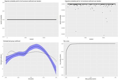
We obtain a 100% true positive rate and a 0% false positive rate in terms of selection, i.e., the two nonzero coefficients are captured in all 100 iterations. Moreover, none of the predictors that originally had zero coefficients are selected. In terms of classification, our method shows 97% sensitivity, 93% specificity, 95% accuracy, and AUC=0.99. Below are the rejection probability plots for ${\text{β}}_2\left(t\right)$ and ${\text{β}}_1\left(t\right)$, of which the first is nonzero and the second is zero in the true model. In addition, we plot the posterior median estimates of the coefficient function with respect to its true values. The ROC curve establishes the differentiating power of our method.

6.4. Example 2 and 3 results

In Example 2, we obtain a 100% true positive rate and a 0.73% false positive rate out of 100 repetitions, with 97% sensitivity and 95% specificity. In Example 3, we achieve a 100% true positive rate and a 0% false positive rate with 98% sensitivity and 97% specificity. We compare our simulation results with those of frequentist group lasso for logistic regression for all the setups above. Our methodology yields the best results in terms of classifying subjects into the right class, far exceeding frequentist group lasso. Although the frequentist group lasso approach successfully identifies the true significant predictors for the model, it also selects many redundant functional predictors that have zero effect on the true model. The false selection of predictors in the model is very high compared to that of our algorithm. The table below summarizes the numerical results of all three aforementioned examples, with comparisons to frequentist group lasso for logistic regression (Figure 1).

Figure 1. Plots based on Example 1.

7. Application on ADNI MRI data

This section reports the results of the application of our proposed method to ADNI data. The MRI data used in all analyses was downloaded from the ADNI database (http://www.adni-info.org/). The fundamental goal of ADNI is to develop a large, standardized neuroimaging database with strong statistical power for research on potential biomarkers in AD incidence, diagnosis, and disease progression. ADNI data available at this time include three projects: ADNI-1, ADNI-GO, and ADNI-2. Starting in 2004, ADNI-1 collected prospective data on cognitive performance, brain structure, and biochemical changes every 6 months. Participants in ADNI-1 included 200 CN, 200 MCI, and 400 AD patients. Then, starting in 2009, ADNI-GO continued the longitudinal study of the existing patients from ADNI-1 and established a new cohort that included early MCI patients, who were enrolled to identify biomarkers manifesting at earlier stages of the disease. ADNI-GO and ADNI-2 together contain additional MRI sequences plus perfusion and diffusion tensor imaging. The volumetric estimation for our data set was performed using FreeSurfer by the UCSF/SF VA Medical Center.

Considerable research has been conducted to develop automatic approaches for patient classification into different clinical groups, with many ADNI studies identifying ROIs associated with different disease stages. A support vector machine (SVM) is a primary tool utilized in many studies to evaluate the patterns in training data sets and to create classifiers to identify new patients. Fan et al. (2008) used neuroimaging data to create a structural phenotypic score reflecting brain abnormalities associated with AD. In classifying AD vs. CN, a positive score in their framework identified AD-like structural brain patterns. Their classifier obtained 94.3% accuracy in AD vs. CN, although their approach used only left and right whole brain volumes as potential predictors. Some researchers have used Bayesian statistical methods in studying Alzheimer's data. Shen et al. (2010) employed a sparse Bayesian learning method, which they named automatic relevance determination (ARD) and predictive ARD, to classify AD patients. This method outperformed an SVM classifier. Yang et al. (2010) proposed a data-driven approach to the automatic classification of MRI scans based on disease stages. Their methodology was broadly divided into two parts. First, they extracted the potentially classifying features from normalized MRI scans using independent component analysis. Next, the separated independent coefficients were applied for the SVM classification of patients. In contrast to this approach, our proposed method selects important components and classifies patients simultaneously. Moreover, we consider multiple brain sub-regions to identify those potential regions whose longitudinal trajectories are specifically related to AD. Another seminal paper by Jack et al. (1999) used MRI-based measurements of hippocampal volume to assess the future risk of conversion from MCI to AD. A bivariate model included hippocampal volume and other factors like age and APOE genotype, but only hippocampal volume was identified as significant. Wang et al. (2014) employed a functional modelling approach using Haar wavelets and lasso regularization to find ROIs in voxel-level data. In that approach, large Haar wavelet coefficients were related to most important features, with a sparse structure among redundant features. The majority of these methods are based on SVM classification, which often uses kernel-based methods for functional smoothing. Casanova et al. (2011) utilized a penalized logistic regression approach, and they calculated estimates using coordinate-wise descent optimization techniques from the GLMNET library. Similarly, our method employs penalized logistic regression with group lasso penalty. However, our approach differs in its use of both functional predictors and a custom algorithm developed in-house.

We consider the longitudinal volume of various brain regions, such as the Para hippocampal gyrus, cerebellar cortices, entorhinal cortex, fusiform gyrus, and precuneus, among many others. Although the accessed ADNI data set includes corresponding volume, surface area, and cortical thickness information, we work with only the volume information to acquire uniformity over longitudinal predictors. Because the brain is divided into right and left hemispheres, the data includes sub-regional brain volumes for both hemispheres. Our main objective is to identify the brain sub-regions whose volumetric trajectories can differentiate AD patients from the normal aging control group. As mentioned in the introduction, dementia is associated with widespread brain atrophy, although the time course and magnitude of shrinkage varies across regions.

The initial sample includes 761 patients' data from the ADNI database, classified as AD, MCI, or CN throughout their visits for the study. We exclude all patients classified as MCI, and any AD or CN patients whose diagnostic status changed over time. This is because our model assumes that response does not depend on time. Of the remaining patients, we include those with data from at least four longitudinal measurement occasions. This yields 296 patients who have at least four data points and unchanging diagnoses of either AD or CN. The final sample is composed of 174 AD patients and 122 normally aging controls. All patients underwent a thorough initial clinical evaluation to measure baseline cognitive and medical scores, including MMSE, the 11-item Alzheimer Cognitive Subscale (ADAS11), and other standardized neuropsychological tests. In addition, at baseline, APOE genotyping information was obtained from patients. Longitudinal structural MRI scans were parcellated into sub-regional brain volumetric measurements. Our initial model includes 49 sub-regional brain volumes chosen by Dr. Andrew Bender, based on knowledge of the extant literature regarding atrophy patterns in AD. Although these 49 sub-regions are not assumed to change in uniform magnitude, the direction of change over time is hypothesized to be consistent (i.e., shrinking). Thus, the model includes 49 longitudinal predictors that we consider as functional predictors. We assume that not all predictors are potential candidates for classifying patients, and that the sparse assumption is valid. However, because some patients' visits were irregular, we do not have an equal number of time points across patients. We start by comparing the baseline measurements between the AD and CN groups, as shown in Tables 1 and 2.

Table 1. Classification and selection performance table.

	Bayesian classification with
	Bayesian Group Lasso
	Sensitivity	Specificity	TPR	FPR	−2 Log likelihood
$\begin{array}{c}\mathrm{E}\mathrm{x}\mathrm{a}\mathrm{m}\mathrm{p}\mathrm{l}\mathrm{e}1\\ n=200\\ p=20\\ t=50\end{array}$	0.97 (0.01)	0.93 (0.01)	1 (0)	0 (0)	3.65
$\begin{array}{c}\mathrm{E}\mathrm{x}\mathrm{a}\mathrm{m}\mathrm{p}\mathrm{l}\mathrm{e}2\\ n=200\\ p=50\\ t=50\end{array}$	0.97 (0.01)	0.95 (0.01)	1 (0)	0.0073 (0.05)	0.219
$\begin{array}{c}\mathrm{E}\mathrm{x}\mathrm{a}\mathrm{m}\mathrm{p}\mathrm{l}\mathrm{e}3\\ n=500\\ p=100\\ t=20\end{array}$	0.98 (0.001)	0.97 (0.01)	1 (0)	0 (0)	6.87
	Logistic regression
	with frequentist group lasso
	Sensitivity	Specificity	TPR	FPR	$-2$ Log likelihood
$\begin{array}{c}\mathrm{E}\mathrm{x}\mathrm{a}\mathrm{m}\mathrm{p}\mathrm{l}\mathrm{e}1\\ n=200\\ p=20\\ t=50\end{array}$	0.92 (0.01)	0.86 (0.01)	1 (0)	0.114 (0.04)	69.23
$\begin{array}{c}\mathrm{E}\mathrm{x}\mathrm{a}\mathrm{m}\mathrm{p}\mathrm{l}\mathrm{e}2\\ n=200\\ p=50\\ t=50\end{array}$	0.81 (0.01)	0.88 (0.01)	1 (0)	0.34 (0.05)	53.66
$\begin{array}{c}\mathrm{E}\mathrm{x}\mathrm{a}\mathrm{m}\mathrm{p}\mathrm{l}\mathrm{e}3\\ n=500\\ p=100\\ t=20\end{array}$	0.91 (0.001)	0.94 (0.001)	1 (0)	0.05 (0.02)	190.23

Note: Simulation result comparisons between Bayesian and Frequentist methods.

Table 2. Patients baseline characteristics.

	AD	CN	p-value
n	174	122
Age (Mean ± sd)	$74.76\pm 7.23$	$75.61\pm 5.45$	0.25
Gender (F/M)	69/105	55/67	0.35
MMSE (Mean ± sd)	$25.43\pm 2.40$	$28.96\pm 1.17$	<.0001
ADAS11 (Mean ± sd)	$14.78\pm 5.44$	$5.95\pm 2.94$	<.0001
APOE $(+/-)$	119/55	30/90	<.0001

Note: Comparison of Baseline Age, Gender ratio, MMSE score, ADAS11 score and APOE ratio between AD and CN groups.

In the next stage, we smooth the longitudinal trajectories for the observed volumes of all brain sub-regions. A simple least squares approximation is sufficient, as we assume that the residuals of the true curve are independently and identically distributed with mean 0 and have constant variance. We use the cubic B-spline basis functions for spline smoothing of observed volumes. Three internal knots are used for spline smoothing with intercept, which gives us seven basis functions. We seek to ensure that the smoothed estimated curve is a good fit for each patient's observed curve. As we do not have a large number of data points for each patient, we do not consider controlling for potential overfitting of our estimated curve. Besides least squares smoothing, functional principle component scores can also be used for this analysis.

Prior to analysis, we scale the brain volumes to the corresponding patients' brain ICV measurement by fitting a simple regression to adjust volume measurements for individual brain volume changes. The aim is to remove systematic variation in brain volumes due to differences in physical size. The formula we use is ${\mathrm{R}\mathrm{O}\mathrm{I}}_{\mathrm{a}\mathrm{d}\mathrm{j}}={\mathrm{R}\mathrm{O}\mathrm{I}}_{\mathrm{v}\mathrm{o}\mathrm{l}}-{\text{β}}_0(\mathrm{I}\mathrm{C}\mathrm{V}-{\mathrm{I}\mathrm{C}\mathrm{V}}_{\mathrm{m}\mathrm{e}\mathrm{a}\mathrm{n}})$, where ${\text{β}}_0$ is the regression coefficient by regressing ${\mathrm{R}\mathrm{O}\mathrm{I}}_{\mathrm{v}\mathrm{o}\mathrm{l}}$ on ICV (Jack et al., 1998; Raz et al., 2005). We adjust or correct the volumes using the above method for each gender group: male and female. Next, we scale the corrected volumes between 0 and 1 to bring all brain regions onto the same scale. We then divide the data set into two parts: two-thirds of the patients are reserved for the training data set (n = 198), and the rest are kept for testing (n = 98). We gather the basis coefficients for each patient in the training data set and use them as predictors for classification. We initialize choice of β with all zero to start iterations. The ${\pi }_0$ probability has a Beta(a,b) distribution with a and b both set up as 1. As a first step, we examine λ using Pólya-Gamma transformation of our sample with a spike-slab penalty on the training data. After estimating λ, we evaluate the remainder of the algorithm on the training data with 30,000 MCMC samples. The first one-third of observations are left out as a burn-in period. We propose a spike-and-slab prior on the β coefficient, which transforms into posterior estimates of zero for most the functional predictors. We run our model 100 times with different training samples to nullify sampling bias in the training and test data. In the 100 iterations, the model does not consistently or uniformly select many of the brain sub-regions; therefore, we choose the brain regions that frequently appear as significant in each iteration. The median thresholding selects the left hippocampus, left lateral orbitofrontal cortex, and left posterior cingulate gyrus with 100% probability. Other brain regions that are selected as important are the right Para hippocampal gyrus, left caudate nucleus, left medial orbitofrontal cortex, left putamen, left superior temporal gyrus, left thalamus, right hippocampus, and right middle temporal gyrus. In Figure 2, we plot the brain volume changes of the left hippocampus, left lateral orbitofrontal cortex, and left posterior cingulate gyrus over time. Orange and green signify the normal aging and dementia group, respectively. The bold thick line represents the mean curve for the corresponding group. The plot shows that there are significant differences in volume between the groups, and our model identifies these regions as significant. In Figure 3, we plot the acceptance probability of the MCMC sample for the left hippocampus and left lateral orbitofrontal brain regions.

Figure 2. Brain volume changes of Left Hippocampus, Left Lateral Orbitofrontal cortex, and Left Posterior Cingulate over time for Normal and Dementia patients.

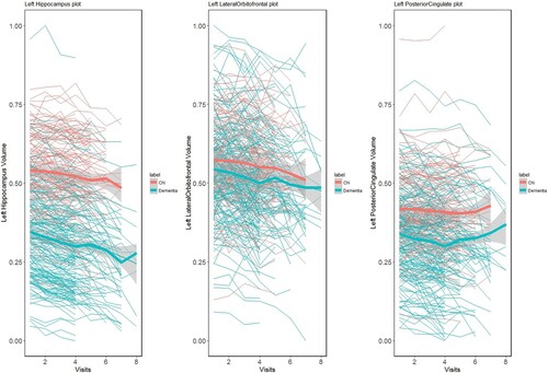
Figure 3. Acceptance probability of MCMC sample for Left Hippocampus and Left-Lateral Orbitofrontal brain regions.

The method classifies patients into the correct group with 77% accuracy. We achieve 72% sensitivity, 85% specificity, and a corresponding AUC of 0.87. We use the median predicted probability from the training sample as the threshold for classification validation. We also test the classification by adding clinical measurements such as the ADAS11 (11-item Alzheimer Cognitive subscale), MMSE scores, ‘CDRSB,’ ‘RAVLT immediate,’ and ‘RAVLT forgetting,’ measured over time. In this classification, we initially select longitudinal brain volumes that are significant, and then we add the clinical variables. We achieve very high classification measures of 97% accuracy, 97% sensitivity, and 98% specificity. If we ignore the MMSE score and run the model with the rest of the functional predictors, we observe similar classification accuracy. In all scenarios, we model diseased patients as 1 and CN as 0 for the interpretation of classification sensitivity/specificity (Figure 4).

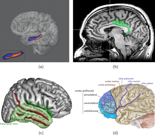
Figure 4. Pictorial representation of selected brain ROI's discriminating diseased group from normal control. (a) Left Hippocampus^a. (b) Posterior Singulate^a. (c) Middle Temporal Gyrus^a and (d) Left lateral orbitofrontal cortex^a.

^a Plot obtained from on-line resources.

In addition to finding functional models of longitudinal trajectories in sub-regional brain volumes to differentiate between the AD and normal groups, we also apply our method for MCI converters vs. MCI nonconverters. We select patients who entered the study as MCI, and we assign the label of MCI nonconverter (MCI-nc) to those who did not transition to AD across all measurement occasions and a label of MCI converter (MCI-c) for any who did transition to AD. The total subsample includes 163 patients who were either MCI-c or MCI-nc. We use three-quarters of the patients to train our model. We note the significant brain ROIs that are selected after 100 iterations. Among the selected ROIs that contribute to classification are the right posterior cingulate gyrus, right superior parietal cortex, right thalamus, right isthmus cingulate gyrus, right fusiform gyrus, left thalamus, and left precuneus. However, the classification performance is not as good as compared to the previous model: 62% accuracy and 0.66 AUC. The biological explanation for this result is critical to acknowledge. The mean difference of functional predictors between MCI-c vs. MCI-nc is not significant for segmenting patients. Moreover, we also neglect some time points' data for this set of patients.

8. Discussion

This paper discusses the use of Bayesian group lasso penalization combined with Pólya-Gamma augmentation to build a simultaneous classification and selection method. The Bayesian spike-and-slab prior helps in identifying functional parameters generated from longitudinal trajectories of multiple brain ROIs, and discriminates the patient group from normal controls. The inclusion of Pólya-Gamma augmentation helps avoid the Metropolis-Hastings algorithm or the incorporation of other expensive sampling algorithms related to latent variables. We consider the longitudinal brain ROI volume measurements as functional predictors, and the cubic basis splines smooth the curves over time. The next steps include using those smoothed functional predictors as discriminating inputs with sparsity assumptions among them.

The consistency property of the posterior distributions provides a theoretical justification regarding the convergence of posterior samples which we sampled for simulation and real data analysis. The posterior distribution $\mathrm{\Pi }(\theta |X_1,\dots ,X_n)$ is said to be consistent at ${\theta }_0$ if it converges to ${\theta }_0$ with some measure. It ensures if we generate enough observations from posterior we would get close to the true value. Our density consistency property ensures that derived posterior distribution will achieve classification consistency for the classification problem we are interested. We would like to mention Doob's theorem regarding this discussion which ensures posterior consistency in Bayesian literature by choosing proper prior. Some priors are problematic which could raise questions regarding any Bayesian methods. We believe our prior selection is reasonable such that posterior consistency holds at every point of the parameter space.

We assumed functional predictors are independent for this paper. In order to capture the dependency between functional predictors, one could introduce a proper prior with some correlation structure between group coefficients. This will increase the model complexity and moreover it would be practically hard to validate these dependency structures in real data analysis. Further research on this topic will definitely be an improvement upon current modeling proposal. Our proposed method performs well on simulated data sets, outperforming available frequentist methods. Furthermore, our method is applied on a data set that has a large number of predictors.

Disclosure statement

No potential conflict of interest was reported by the author(s).

Additional information

Funding

This work was supported by Directorate for Mathematical and Physical Sciences [1924724].

Appendix: Posterior derivations

Let us define $B\left(r_n\right)=\underset{\gamma =\gamma \left(r_n\right)}{sup}\mathrm{C}\mathrm{h}\left(G_{r_n}^{-1}\right)$ and $\overline{B}\left(r_n\right)=\underset{\gamma =\gamma \left(r_n\right)}{sup}\mathrm{C}\mathrm{h}\left(G_{r_n}\right)$ where $G_{r_n}=\mathrm{d}\mathrm{i}\mathrm{a}\mathrm{g}({\tau }_1^{\ast }{I}_q,\dots ,{\tau }_{r_n}^{\ast }{I}_q)$. $B\left(r_n\right)$ is the largest eigenvalues of $G_{r_n}$ and $D\left(R\right)=1+R.\underset{|h|\le R}{sup}|a^{\mathrm{\prime }}\left(h\right)|\underset{|h|\le R}{sup}|\psi \left(h\right)|$. Let ${ϵ}_n\to (0,1]$ with $n{ϵ}_n^2\succ 1$ and assume the below conditions hold which come from Jiang (2007) paper.

Conditions: $\begin{array}{rl}& \left(\mathrm{i}\right)p_n\log \left(1/{ϵ}_n^2\right)\prec n{ϵ}_n^2,\\ & \left(\mathrm{i}\mathrm{i}\right)p_n\log \left(p_n\right)\prec n{ϵ}_n^2,\\ & \left(\mathrm{i}\mathrm{i}\mathrm{i}\right)p_n\log \left(D\left(\frac{p_n}{{\lambda }_n}\overline{B}\right(r_n\left)n{ϵ}_n^2\right)\right)\succ n{ϵ}_n^2,\\ & \left(\mathrm{i}\mathrm{v}\right)r_n\succ p_n,\\ & \left(\mathrm{v}\right)r_n\log \left(\overline{B}\right(r_n\left)n\right)\succ n{ϵ}_n^2\mathrm{a}\mathrm{n}\mathrm{d}\mathrm{\Delta }\left(r_n\right)\succ n{ϵ}_n^2,\\ & \left(\mathrm{v}\mathrm{i}\right)\log \left(\frac{r_n}{p_n}\right)\le -\frac{4n{ϵ}_n^2}{p_n}.\end{array}$

Proof

Proof of Condition I

If $\psi \left(u\right)={\mathrm{e}}^u/(1+{\mathrm{e}}^u)$, then $\begin{array}{rl}& w\left(u\right)=\log \left[\psi \right(u\left)/\right(1-\psi \left(u\right)\left)\right]=u\\ & ⟹w^{\mathrm{\prime }}\left(u\right)=1\\ & ⟹|w^{\mathrm{\prime }}\left(u\right)|\le C^q\text{■}\end{array}$

Proof

Proof of Condition S

The proof starts with defining set and notations used in condition S. Let $r_n$ be a large integer $>0$ and η is small $>0$. Then $\begin{array}{rl}S(r_n,\eta )& =\left\{\right(\gamma ,{\text{β}}_{\gamma }\left)\right):\gamma =\gamma \left(r_n\right),{\text{β}}_{\gamma }\in M(r_n,n)\},\\ M(r_n,n)& =\left\{\right(b_1,\dots ,b_{r_n}{)}^{\mathrm{\top }}:b_j\in {\text{β}}_j\pm \frac{n{ϵ}_n^2}{r_n},j=1,\dots ,r_n\}.\end{array}$Here $r_n$ is the model size and $\gamma \left(r_n\right)=(1,2,\dots ,r_n,0,\dots .)$ is an increasing sequence whose first $r_n$ components take value 1.

Let, $1\prec r_n\prec min(p_n,n/\log (p_n\left)\right)$ and $\sum _{j=1}^{\mathrm{\infty }}||{\text{β}}_j|{|}_2<\mathrm{\infty }$. $\begin{array}{rl}& {\pi }_n[{\text{β}}_{\gamma }\in {\text{β}}_j\pm \frac{n{ϵ}_n^2}{r_n}|\gamma =\gamma (r_n\left)\right]\\ & \ge \prod _{j=1}^{r_n}[\frac{({\lambda }_n^2{)}^{\left(q/2\right)}}{(2\pi {)}^{(q-1)/2}}\exp (-{\lambda }_n\sqrt{{\overline{\text{β}}}_j^{\mathrm{\top }}{\overline{\text{β}}}_j})\left(\frac{n{ϵ}_n^2}{r_n}\right)],\end{array}$where ${\overline{\text{β}}}_j$ is some intermediate value which achieves the minimum density over $({\text{β}}_j\pm \frac{n{ϵ}_n^2}{r_n}{)}_{j\in \gamma \left(r_n\right)}$. Then, ${\lambda }_n\sum _{j=1}^{r_n}\sqrt{{\overline{\text{β}}}_j^{\mathrm{\top }}{\overline{\text{β}}}_j}\le C_{1}B\left(r_n\right),$as $\sum _{j=1}^{r_n}\sqrt{{\overline{\text{β}}}_j^{\mathrm{\top }}{\overline{\text{β}}}_j}\le \underset{n\to \mathrm{\infty }}{lim}\sum _{j=1}^{p_n}\sqrt{{\overline{\text{β}}}_j^{\mathrm{\top }}{\overline{\text{β}}}_j}+\frac{n{ϵ}_n^2}{r_n}$ is bounded. In addition we can show that, $\prod _{j=1}^{r_n}\frac{({\lambda }_n^2{)}^{\left(q/2\right)}}{(2\pi {)}^{(q-1)/2}}\ge \exp (-C_2{r}_n-C_3{r}_n\log (\overline{B}\left(r_n\right)),$where $\overline{B}\left(r_n\right)=\underset{\gamma =\gamma \left(r_n\right)}{sup}\mathrm{C}\mathrm{h}\left(G_{r_n}\right)$. Therefore, $\begin{array}{rl}& {\pi }_n[{\text{β}}_{\gamma }\in {\text{β}}_j\pm \frac{n{ϵ}_n^2}{r_n}|\gamma =\gamma (r_n\left)\right]\\ & \ge \exp (\phantom{\left(\frac{r_n}{n{ϵ}_n^2}\right)}-C_2{r}_n-C_3{r}_n\log (\overline{B}\left(r_n\right)\\ & -C_{1}B\left(r_n\right)-r_n\log \left(\frac{r_n}{n{ϵ}_n^2}\right))\\ & \ge \exp (-cn{ϵ}_n^2).\end{array}$To prove the prior condition, let ${\overline{r}}_n$ such that $r_n<{\overline{r}}_n\le p_n$ and ${\overline{r}}_n\prec n/\ln \left(p_n\right)$. For our model we have placed ${\pi }_{0,n}\sim \mathrm{B}\mathrm{e}\mathrm{t}\mathrm{a}\mathrm{d}\mathrm{i}\mathrm{s}\mathrm{t}\mathrm{r}\mathrm{i}\mathrm{b}\mathrm{u}\mathrm{t}\mathrm{i}\mathrm{o}\mathrm{n}$ which is equivalent way of proposing Bernoulli distribution on $\gamma =\gamma \left(r_n\right)$ where $\gamma \left(r_n\right)\sim \mathrm{B}\mathrm{e}\mathrm{r}\mathrm{n}\mathrm{o}\mathrm{u}\mathrm{l}\mathrm{l}\mathrm{i}\left({\pi }_{0,n}\right)$ (Smith & Kohn, 1996).

Now, $\ln {\pi }_n=r_n\ln {\pi }_{0,n}+(p_n-r_n)\ln (1-{\pi }_{0,n}).$If $r_n\approx p_n{\lambda }_n$ then for ${\pi }_{0,n}=r_n/p_n$ small and $1\prec r_n\prec min(p_n,n/\ln p_n)$ $\begin{array}{rl}& ⟹\ln {\pi }_n\ge -r_n\ln p_n>-cn{ϵ}_n^2\text{for large }n\\ & ⟹{\pi }_n[\gamma =\gamma (r_n\left)\right]>\exp (-cn{ϵ}_n^2),\end{array}$satisfying condition S.

Proof

Proof of Condition L

Let us assume $D\left(R\right)=1+R.\underset{|h|\le R}{sup}|a^{\mathrm{\prime }}\left(h\right)|\underset{|h|\le R}{sup}|\psi \left(h\right)|$ and there exists some $C_n$ such that $\begin{array}{rl}{\overline{r}}_n\ln \left(\frac{1}{{ϵ}_n^2}\right)& \prec n{ϵ}_n^2,\\ {\overline{r}}_n\ln \left(p_n\right)& \prec n{ϵ}_n^2,\\ {\overline{r}}_n\ln D\left({\overline{r}}_n{C}_n\right)& \prec n{ϵ}_n^2.\end{array}$Then, $\begin{array}{rl}{\pi }_n(|\gamma |>{\overline{r}}_n)& ={\pi }_n(|\gamma |=p_n)={\left(\frac{r_n}{p_n}\right)}^{p_n}\\ & ⟹\ln \left({\pi }_n\right(|\gamma |>{\overline{r}}_n)\\ & =p_n\ln \left(\frac{r_n}{p_n}\right)\le -cn{ϵ}_n^2\\ & ⟹{\pi }_n(|\gamma |>{\overline{r}}_n)\le {\mathrm{e}}^{-cn{ϵ}_n^2}.\end{array}$Next, $\begin{array}{rl}{\pi }_n(||{\text{β}}_j|{|}_2>t|\gamma )& \propto {\int }_t^{\mathrm{\infty }}{\mathrm{e}}^{-{\lambda }_n\sqrt{{\text{β}}_j^{\mathrm{\top }}{\text{β}}_j}}\mathrm{d}{\text{β}}_j\\ & \le \frac{1}{{\lambda }_n}{\mathrm{e}}^{-{\lambda }_{n}t}.\end{array}$If $t=C_n=\frac{cn{ϵ}_n^2}{{\lambda }_n}$ and $n{ϵ}_n^2\succ 1$, then $\frac{1}{{\lambda }_n}{\mathrm{e}}^{-{\lambda }_{n}t}\le {\mathrm{e}}^{-cn{ϵ}_n^2},\mathrm{a}\mathrm{s}{\lambda }_n\ge 1,$satisfying condition (L).

References

- Adaszewski, S., Dukart, J., Kherif, F., Frackowiak, R., & Draganski, B. (2013). How early can we predict Alzheimer's disease using computational anatomy? Neurobiology of Aging, 34(12), 2815–2826. https://doi.org/10.1016/j.neurobiolaging.2013.06.015
- Arlt, S., Buchert, R., Spies, L., Eichenlaub, M., Lehmbeck, J. T., & Jahn, H. (2013). Association between fully automated MRI-based volumetry of different brain regions and neuropsychological test performance in patients with amnestic mild cognitive impairment and Alzheimer's disease. European Archives of Psychiatry and Clinical Neuroscience, 263(4), 335–344. https://doi.org/10.1007/s00406-012-0350-7
- Casanova, R., Wagner, B., Whitlow, C. T., Williamson, J. D., S. A. Shumaker, Maldjian, J. A., & Espeland, M. A. (2011). High dimensional classification of structural MRI Alzheimer's disease data based on large scale regularization. Frontiers in Neuroinformatics, 5, 22. https://doi.org/10.3389/fninf.2011.00022
- Casella, G., Ghosh, M., Gill, J., & Kyung, M. (2010). Penalized regression, standard errors, and Bayesian lassos. Bayesian Analysis, 5(2), 369–411.
- Fan, Y., Batmanghelich, N., Clark, C. M., & Davatzikos, C., and Alzheimer's Disease Neuroimaging Initiative and others (2008). Spatial patterns of brain atrophy in MCI patients, identified via high-dimensional pattern classification, predict subsequent cognitive decline. NeuroImage, 39(4), 1731–1743. https://doi.org/10.1016/j.neuroimage.2007.10.031
- Fan, Y., James, G. M., & Radchenko, P. (2015). Functional additive regression. The Annals of Statistics, 43(5), 2296–2325. https://doi.org/10.1214/15-AOS1346
- George, E. I., & McCulloch, R. E. (1993). Variable selection via Gibbs sampling. Journal of the American Statistical Association, 88(423), 881–889. https://doi.org/10.1080/01621459.1993.10476353
- George, E. I., & McCulloch, R. E. (1997). Approaches for Bayesian variable selection. Statistica Sinica, 7, 339–373. https://www.jstor.org/stable/24306083
- Hobert, J. P., & Geyer, C. J. (1998). Geometric ergodicity of Gibbs and block Gibbs samplers for a hierarchical random effects model. Journal of Multivariate Analysis, 67(2), 414–430. https://doi.org/10.1006/jmva.1998.1778
- Ishwaran, H., & Rao, J. S., et al. (2005). Spike and slab variable selection: Frequentist and bayesian strategies. The Annals of Statistics, 33(2), 730–773. https://doi.org/10.1214/009053604000001147
- Jack, C. R., Petersen, R. C., Xu, Y., O'Brien, P. C., Smith, G. E., Ivnik, R. J., E. G. Tangalos, & Kokmen, E. (1998). Rate of medial temporal lobe atrophy in typical aging and Alzheimer's disease. Neurology, 51(4), 993–999. https://doi.org/10.1212/WNL.51.4.993
- Jack, C. R., Petersen, R. C., Xu, Y. C., O'Brien, P. C., Smith, G. E., Ivnik, R. J., Boeve, B. F., Waring, S. C., Tangalos, E. G., & Kokmen, E. (1999). Prediction of ad with MRI-based hippocampal volume in mild cognitive impairment. Neurology, 52(7), 1397–1397. https://doi.org/10.1212/WNL.52.7.1397
- James, G. M. (2002). Generalized linear models with functional predictors. Journal of the Royal Statistical Society: Series B (Statistical Methodology), 64(3), 411–432. https://doi.org/10.1111/rssb.2002.64.issue-3
- Jiang, W. (2006). On the consistency of bayesian variable selection for high dimensional binary regression and classification. Neural Computation, 18(11), 2762–2776. https://doi.org/10.1162/neco.2006.18.11.2762
- Jiang, W. (2007). Bayesian variable selection for high dimensional generalized linear models: Convergence rates of the fitted densities. The Annals of Statistics, 35(4), 1487–1511. https://doi.org/10.1214/009053607000000019
- Johnstone, I. M., & Silverman, B. W. (2004). Needles and straw in haystacks: Empirical Bayes estimates of possibly sparse sequences. The Annals of Statistics, 32(4), 1594–1649. https://doi.org/10.1214/009053604000000030
- Lee, S. H., Bachman, A. H., Yu, D., Lim, J., & Ardekani, B. A., and Alzheimer's Disease Neuroimaging Initiative and others (2016). Predicting progression from mild cognitive impairment to Alzheimer's disease using longitudinal callosal atrophy. Alzheimer's & Dementia: Diagnosis, Assessment & Disease Monitoring, 2(1), 68–74. https://doi.org/10.1016/j.dadm.2016.01.003
- Leng, C., Tran, M.-N., & Nott, D. (2014). Bayesian adaptive lasso. Annals of the Institute of Statistical Mathematics, 66(2), 221–244. https://doi.org/10.1007/s10463-013-0429-6
- Li, Q., Lin, N. (2010). The bayesian elastic net. Bayesian Analysis, 5(1), 151–170. https://doi.org/10.1214/10-BA506
- Majumder, A. (2017). Variable selection in high-dimensional setup: A detailed illustration through marketing and MRI data. Michigan State University.
- Meier, L., S. Van De Geer, & Bühlmann, P. (2008). The group lasso for logistic regression. Journal of the Royal Statistical Society: Series B (Statistical Methodology), 70(1), 53–71. https://doi.org/10.1111/j.1467-9868.2007.00627.x
- Misra, C., Fan, Y., & Davatzikos, C. (2009). Baseline and longitudinal patterns of brain atrophy in mci patients, and their use in prediction of short-term conversion to ad: Results from adni. NeuroImage, 44(4), 1415–1422. https://doi.org/10.1016/j.neuroimage.2008.10.031
- Müller, H.-G. (2005). Functional modelling and classification of longitudinal data. Scandinavian Journal of Statistics, 32(2), 223–240. https://doi.org/10.1111/sjos.2005.32.issue-2
- Park, T., & Casella, G. (2008). The bayesian lasso. Journal of the American Statistical Association, 103(482), 681–686. https://doi.org/10.1198/016214508000000337
- Polson, N. G., Scott, J. G., & Windle, J. (2013). Bayesian inference for logistic models using pólya–gamma latent variables. Journal of the American Statistical Association, 108(504), 1339–1349. https://doi.org/10.1080/01621459.2013.829001
- Raz, N., Lindenberger, U., Rodrigue, K. M., Kennedy, K. M., Head, D., Williamson, A., Dahle, C., Gerstorf, D., & Acker, J. D. (2005). Regional brain changes in aging healthy adults: General trends, individual differences and modifiers. Cerebral Cortex, 15(11), 1676–1689. https://doi.org/10.1093/cercor/bhi044
- Seixas, F. L., Zadrozny, B., Laks, J., Conci, A., & Saade, D. C. M. (2014). A bayesian network decision model for supporting the diagnosis of dementia, Alzheimer's disease and mild cognitive impairment. Computers in Biology and Medicine, 51(8), 140–158. https://doi.org/10.1016/j.compbiomed.2014.04.010
- Shen, L., Qi, Y., Kim, S., Nho, K., Wan, J., Risacher, S. L., & Saykin, A. J., and others. (2010). Sparse bayesian learning for identifying imaging biomarkers in ad prediction. In International Conference on Medical Image Computing and Computer-Assisted Intervention (pp. 611–618). Springer.
- Shi, G. (2017). Bayesian variable selection: Extensions of nonlocal priors. Michigan State University. Statistics.
- Smith, M., & Kohn, R. (1996). Nonparametric regression using Bayesian variable selection. Journal of Econometrics, 75(2), 317–343. https://doi.org/10.1016/0304-4076(95)01763-1
- Wang, X., Nan, B., Zhu, J., & Koeppe, R. (2014). Regularized 3d functional regression for brain image data via haar wavelets. The Annals of Applied Statistics, 8(2), 1045. https://doi.org/10.1214/14-AOAS736
- Windle, J., Polson, N. G., & Scott, J. G. (2014). Sampling polya-gamma random variates: Alternate and approximate techniques. arXiv preprint arXiv:1405.0506.
- Xu, X., Ghosh, M. (2015). Bayesian variable selection and estimation for group lasso. Bayesian Analysis, 10(4), 909–936. https://doi.org/10.1214/14-BA929
- Yang, W., Chen, X., Xie, H., & Huang, X. (2010). Ica-based automatic classification of magnetic resonance images from adni data. In Life System Modeling and Intelligent Computing (pp. 340–347). Springer.
- Zhang, D., & Shen, D., and Alzheimer's Disease Neuroimaging Initiative. (2012). Predicting future clinical changes of MCI patients using longitudinal and multimodal biomarkers. PloS One, 7(3), e33182. https://doi.org/10.1371/journal.pone.0033182
- Zhu, H., Vannucci, M., & Cox, D. D. (2010). A Bayesian hierarchical model for classification with selection of functional predictors. Biometrics, 66(2), 463–473. https://doi.org/10.1111/j.1541-0420.2009.01283.x