
 ?Mathematical formulae have been encoded as MathML and are displayed in this HTML version using MathJax in order to improve their display. Uncheck the box to turn MathJax off. This feature requires Javascript. Click on a formula to zoom.
Abstract
The Lomax distribution is an important member in the distribution family. In this paper, we systematically develop an objective Bayesian analysis of data from a Lomax distribution. Noninformative priors, including probability matching priors, the maximal data information (MDI) prior, Jeffreys prior and reference priors, are derived. The propriety of the posterior under each prior is subsequently validated. It is revealed that the MDI prior and one of the reference priors yield improper posteriors, and the other reference prior is a second-order probability matching prior. A simulation study is conducted to assess the frequentist performance of the proposed Bayesian approach. Finally, this approach along with the bootstrap method is applied to a real data set.
1. Motivation
A random variable is said to be distributed as a Lomax distribution if its density function has the following form:
(1)
(1) where
is the shape parameter and
is the scale parameter. The distribution is originally introduced in Lomax (Citation1954) for the analysis of business failure data. Since then, the Lomax model has been widely applied in many other fields. For example, Atkinson and Harrison (Citation1978) utilized the Lomax distribution to model personal wealth data; Bain and Engelhardt (Citation1992) found that the Lomax distribution provided a good model for biomedical problems, such as survival time following a heart transplant; Holland et al. (Citation2006) applied the Lomax distribution to model the distribution of the sizes of computer files on servers; and Marshall and Olkin (Citation2007) showed that the Lomax distribution can be applied as a lifetime distribution. For some extensions of the Lomax distribution, one is referred to Nayak (Citation1987), Roy and Gupta (Citation1996), Nadarajah (Citation2005), Lemonte and Cordeiro (Citation2013), Kang et al. (Citation2021) among others.
For the Lomax model (Equation1(1)
(1) ), there is no closed-form expression for the classical maximum likelihood estimator (MLE). More importantly, as pointed out by Deville (Citation2016), the MLE does not exist if the sample coefficient of variation
, which was also analyzed in detail in Chakraborty (Citation2019). In addition, a simulation study indicates that the probability of
is not negligible. For example, when
and n = 20, the empirical probability of
is as high as 0.25. In this sense, the MLE method is not applicable under these cases.
Thus, it is natural to consider Bayesian estimation for the parameters in model (Equation1
(1)
(1) ). In a Bayesian paradigm, the specification of a prior distribution is one of the most important problems. We first consider the following vague prior for
, that is,
(2)
(2) where
is a hyperparameter. That is to say, the ‘marginal’ prior for α is a gamma distribution. It is shown that the posterior distribution of
is proper for any
(see the Appendix for proofs), where
is the sample. To assess the sensitivity of the corresponding Bayesian estimation with respect to the hyperparameter τ, we conduct a sensitivity analysis here.
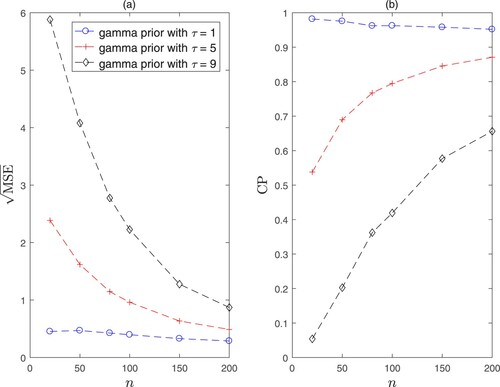
The values of are set as
, and τ is set as 1, 5 and 9, respectively. The empirical square root of the mean squared error (
) and coverage probability (CP) of the Bayesian estimation with respect to the sample size n are shown in Figure . It can be observed that the performance of the MSE and CP based on the prior
is very sensitive to the choice of the hyperparameter τ, which makes it difficult to specify
in applications. Obviously, if one is interested in making an optimal decision based on his/her beliefs, such a (subjective) prior could be appropriate.
Figure 1. Square root of the mean squared error and coverage probability of the Bayesian estimation of α based on the gamma priors with
(circle),
(cross), and
(diamond). Panel (a) is for the square root of mean squared error, and panel (b) is for the coverage probability.
Based on the above motivation, we propose an objective Bayesian analysis for the Lomax model in this paper, particularly when there is little prior information on the parameters. As we know, one of the most appealing features of the objective Bayesian analysis is to use noninformative priors. In the work of Ferreira et al. (Citation2016, Citation2020), Jeffreys prior and independent Jeffreys prior (i.e., one of the reference priors) were considered. In this paper, we propose a more systematic and deeper analysis based on an extensive class of objective priors including probability matching priors, the maximal data information (MDI) prior, Jeffreys prior and reference priors.
The remainder of this paper is organized as follows. In Section 2, noninformative priors, including probability matching priors, the MDI prior, Jeffreys prior and reference priors are derived. Moreover, the posterior propriety under each prior is validated. In Section 3, a simulation study is conducted to evaluate the frequentist properties of Bayesian estimates based on the noninformative priors. In Section 4, the proposed Bayesian approach is applied to analyze a real data set. Some concluding remarks are given in Section 5.
2. Noninformative priors and their properties
In this section, we derive some important noninformative priors for the parameters , which contain probability matching priors, the MDI prior, Jeffreys prior and reference priors.
2.1. Probability matching priors
The rationale behind a probability matching prior is that a noninformative prior should provide inferences that are similar to those obtained from a frequentist perspective, such as in terms of credible versus confidence intervals. In this perspective, a probability matching prior is a prior such that the posterior coverage probability of Bayesian credible interval matches the corresponding frequentist coverage probability (Consonni et al., Citation2018).
Given a prior for the parameters
, suppose that ϕ is the parameter of interest, and
is the
-th percentile of the marginal posterior distribution of ϕ. Then,
is called a second-order probability matching prior if
holds for all
, see Datta and Mukerjee (Citation2004) for more details.
For the parameters α and β in the Lomax model (Equation1(1)
(1) ), we have the following theorem.
Theorem 2.1
| (a) | When α is the parameter of interest and β is the nuisance parameter, the second-order probability matching prior has the form of
| ||||
| (b) | When β is the parameter of interest and α is the nuisance parameter, the second-order probability matching prior is given by
| ||||
2.2. The MDI prior
Lindley (Citation1956) applied the Shannon entropy to develop an information theoretic analysis of the structure of Bayesian modelling. This prompted the works on the definition of the least informative prior distribution based on some definitions of the amount of information. Zellner (Citation1977) proposed an important noninformative prior, which is called the MDI prior. Zellner (Citation1977) proved that using this prior could emphasize the information in the likelihood function. Therefore, the information in the prior is weak compared with that in the data (Ramos et al., Citation2018).
For the Lomax model (Equation1(1)
(1) ), we have the following result, the proofs of which are deferred to the Appendix.
Theorem 2.2
| (a) | The MDI prior for the parameters | ||||
| (b) | For any | ||||
2.3. Jeffreys prior
Jeffreys prior is probably the most popular noninformative prior method among practitioners. According to Jeffreys (Citation1961), Jeffreys prior is proportional to the square root of the determinant of the Fisher information matrix. Besides being parametrization invariant, Jeffreys prior enjoys many optimality properties in the absence of nuisance parameters. It maximizes the asymptotic divergence between the prior and the posterior under several different metrics. However, Jeffreys prior also has some potential drawbacks. Particularly, in the multidimensional case, its use may lead to incoherence and paradoxes. See Consonni et al. (Citation2018) for more discussions.
For the Lomax model (Equation1(1)
(1) ), Jeffreys prior for the parameters
has the following form:
(6)
(6) And it was shown in Ferreira et al. (Citation2020) that, for any
, the posterior distribution under
is proper.
By Theorem 2.1, we have the following theorem.
Theorem 2.3
Regardless of whether α is the parameter of interest or β is the parameter of interest, is always not a second-order probability matching prior.
2.4. Reference priors
Reference analysis uses information-theoretical concepts to precisely define the objective prior, which should be maximally dominated by the data, in the sense of maximizing the missing information on the parameters (Berger et al., Citation2009). The original formulation of reference priors was introduced in Bernardo (Citation1979), which was largely informal. Berger and Bernardo (Citation1992) gave more precise definitions of the sequential reference process in continuous multiparameter problems. In addition, a rigorous general definition of reference priors was formally given in Berger et al. (Citation2009) for one block of parameters.
As we know, reference priors separate the parameters into different ordering groups of interest. For the ordering group , it was shown in Ferreira et al. (Citation2020) that the reference prior is
(7)
(7) Furthermore, for any
, the posterior distribution under the reference prior
is improper.
For the ordering group , we have the following theorem.
Theorem 2.4
| (a) | The reference prior under the ordering group | ||||
| (b) | For n = 1, the posterior distribution under the reference prior | ||||
| (c) | The prior | ||||
The proofs of Theorem 2.4 are also deferred to the Appendix. It follows from Theorems 2.2–2.4 that only Jeffreys prior and the reference prior
enable posterior inferences. However,
is a second-order probability matching prior while
is not. In this sense,
is recommended for potential users. In fact, this is also verified in the following numercial studies.
3. Simulation study
To evaluate the frequentist performance of the Bayesian estimation based on and
, we simulate data from the Lomax model (Equation1
(1)
(1) ) with different true values of the parameters α and β and different sample sizes n. Then, posterior samples are drawn from the joint posterior distribution of α and β by using the random-walk Metropolis algorithm in Roberts et al. (Citation1997). For each chain, the sample size is 50000 after 5000 burn-in samples. By choosing samples with jump of 10, a final chain of 5000 values is obtained. In order to make the estimation more robust, we take the posterior median as the Bayesian estimator for each parameter. The process is replicated 5000 times. Thus, we can obtain estimated mean squared errors and coverage probabilities of credible intervals (CIs).
The empirical results of the MSE and CP for the 95% CIs are listed in Table , where the estimated probabilities that the sample coefficient of variation is less than 1 are also associated. From Table , the following observations can be found.
As is expected, the MSEs of the Bayesian estimators decrease as the sample size increases. Meanwhile, the CPs of the 95% CIs approach the nominal level of 0.95.
The larger the value of α is, the higher the probability
. For each parameter, the larger the true value is, the larger the corresponding MSE.
According to both the MSE and CP, the performance of the Bayesian estimators under the reference prior
Table 1. Empirical MSEs and CPs (within parentheses) of Bayesian estimators based on the priors and
.
4. Real data analysis
Now we apply the proposed Bayesian approach to analyze a sample of computer file sizes (in bytes) for 269 files with the *.ini extension on a Windows-based personal computer. The data are available on the website http://web.uvic.ca/∼dgiles/downloads/data. The data were also analyzed by Holland et al. (Citation2006) and Ferreira et al. (Citation2016), where the Lomax distribution was shown to appropriately fit this data.
For comparison purposes, the parametric bootstrap and the Bayesian approaches based on the Jeffreys prior and the reference prior
are included here. The parametric bootstrap is based on the MLE since the sample coefficient of variation
is greater than 1 here. The estimators along with the corresponding standard deviation (SD) and 95% confidence/credible interval (CI) for α and β are listed in Table . It can be seen from Table that the Bayesian estimates of β are much more accurate than those of the parametric bootstrap according to the SD and the width of the CI. In addition, the performances of the two Bayesian estimates are close to each other, although the prior
behaves slightly better than
. To conclude, it is noted that our results are close to those in Ferreira et al. (Citation2016) with respect to Jeffreys prior.
Table 2. Summary of the parametric bootstrap and the Bayesian estimates.
5. Concluding remarks
In this paper, objective Bayesian methods are developed to make inferences on the parameters of a Lomax distribution. Compared with the work in the literature, our contribution lies in the following points. First, we consider a larger class of noninformative priors, which includes probability matching priors, the MDI prior and both of reference priors. Second, it is revealed that one of reference priors is a second-order probability matching prior while Jeffreys prior is not. Third, we clarify that the MLE does not exist if the sample coefficient of variation , and also consider the probability of such phenomenon in the simulation study. As a result, it is feasible to use objective Bayesian analysis for the Lomax distribution in practice.
Acknowledgments
The authors would like to thank the Editor, the Associate Editor and the anonymous Reviewers for their valuable comments and suggestions on earlier versions of this paper.
Disclosure statement
No potential conflict of interest was reported by the author(s).
Additional information
Funding
References
- Atkinson, A. B., & Harrison, A. J. (1978). Distribution of personal wealth in Britain. Cambridge University Press.
- Bain, L. J., & Engelhardt, M. (1992). Introduction to probability and mathematical statistics. PWSKENT Publishing Company.
- Berger, J. O., & Bernardo, J. M. (1992). Ordered group reference priors with application to the multinomial problem. Biometrika, 79(1), 25–37. https://doi.org/10.1093/biomet/79.1.25
- Berger, J. O., Bernardo, J. M., & Sun, D. C. (2009). The formal definition of reference priors. The Annals of Statistics, 37(2), 905–938. https://doi.org/10.1214/07-AOS587
- Bernardo, J. M. (1979). Reference posterior distributions for Bayesian inference (with discussion). Journal of the Royal Statistical Society: Series B (Methodological), 41(2), 113–147. https://doi.org/10.1111/j.2517-6161.1979.tb01066.x
- Chakraborty, T. (2019). An analysis of the maximum likelihood estimates for the Lomax distribution. ArXiv: 1911.12612v2, 1–14.
- Consonni, G., Fouskakis, D., Liseo, B., & Ntzoufras, I. (2018). Prior distributions for objective Bayesian analysis. Bayesian Analysis, 13(2), 627–679. https://doi.org/10.1214/18-BA1103
- Datta, G. S., & Mukerjee, R. (2004). Probability matching priors: Higher order asymptotics. Lecture Notes in Statistics. Sringer.
- Deville, Y. (2016). Renext: Renewal method for extreme values extrapolation (p. 25). https://cran.r-project.org/web/packages/Renext/Renext.pdf.
- Ferreira, P. H., Gonzales, J. F. B., Tomazella, V. L. D., Ehlers, R. S., Louzada, F., & Silva, E. B. (2016). Objective Bayesian analysis for the Lomax distributionms. ArXiv: 1602.08450v1, 1–19.
- Ferreira, P. H., Ramos, E., Ramos, P. L., Gonzales, J. F. B., Tomazella, V. L. D., R. S. Ehlers, Silva, E. B., & Louzad, F. (2020). Objective Bayesian analysis for the Lomax distribution. Statistics & Probability Letters, 159, Article 108677. https://doi.org/10.1016/j.spl.2019.108677
- Holland, O., Golaup, A., & Aghvami, A. H. (2006). Traffic characteristics of aggregated module downloads for mobile terminal reconfiguration. IEEE Proceedings: Communications, 153(5), 683–690. https://doi.org/10.1049/ip-com:20045155
- Jeffreys, H. (1961). Theory of probability (3rd ed.). Oxford University Press.
- Kang, S. G., Lee, W. D., & Kim, Y. (2021). Posterior propriety of bivariate lomax distribution under objective priors. Communication in Statistics – Theory and Methods, 50(9), 2201–2209. https://doi.org/10.1080/03610926.2019.1662049
- Lemonte, A. J., & Cordeiro, G. M. (2013). An extended Lomax distribution. Statistics, 47(4), 800–816. https://doi.org/10.1080/02331888.2011.568119
- Lindley, D. V. (1956). On a measure of the information provided by an experiment. The Annals of Mathematical Statistics, 27(4), 986–1005. https://doi.org/10.1214/aoms/1177728069
- Lomax, K. (1954). Business failures: Another example of the analysis of failure data. Journal of the American Statistical Association, 49(268), 847–852. https://doi.org/10.1080/01621459.1954.10501239
- Marshall, A. W., & Olkin, I. (2007). Life distributions: Structure of nonparametric, semiparametric, and parametric families. Springer.
- Nadarajah, S. (2005). Sums, products, and ratios for the bivariate Lomax distribution. Computational Statistics & Data Analysis, 49(1), 109–129. https://doi.org/10.1016/j.csda.2004.05.003
- Nayak, T. K. (1987). Multivariate Lomax distribution: Properties and usefulness in reliability theory. Journal of Applied Probability, 24(1), 170–177. https://doi.org/10.2307/3214068
- Peers, H. W. (1965). On confidence sets and Bayesian probability points in the case of several parameters. Journal of the Royal Statistical Society: Series B (Methodological), 27(1), 9–16. https://doi.org/10.1111/j.2517-6161.1965.tb00581.x
- Ramos, P. L., Louzada, F., & Ramos, E. (2018). Posterior properties of the Nakagami-m distribution using non-informative priors and applications in reliability. IEEE Transactions on Reliability, 67(1), 105–117. https://doi.org/10.1109/TR.24
- Roberts, G. O., Gelman, A., & Gilks, W. R. (1997). Weak convergence and optimal scaling of random walk metropolis algorithms. Annals of Applied Probability, 7(1), 110–120 . http://doi.org/10.1214/aoap/1034625254
- Roy, D., & Gupta, R. P. (1996). Bivariate extension of Lomax and finite range distributions through characterization approach. Journal of Multivariate Analysis, 59(1), 22–33. https://doi.org/10.1006/jmva.1996.0052
- Zellner, A. (1977). Maximal data information prior distributions. In A. Aykac & C. Brumat (Eds.), New developments in the applications of Bayesian methods (pp. 211–232). North-Holland.
Appendix
Proof
Proof of the posterior propriety of
The joint posterior density of based on the prior
is given by
Denote
. Then we have
where
is the Beta function. Let
Then, it can be seen that
Thus,
for any
. Consequently, the posterior distribution of
is proper.
Proof
Proof of Theorem 2.1
According to Peers (Citation1965), the second-order probability matching prior satisfies the following partial differential equation:
the solution of which is given by formula (Equation3
(3)
(3) ). Similarly, the second-order probability matching prior
is such that
and the solution of this equation is given by formula (Equation4
(4)
(4) ).
Proof
Proof of Theorem 2.2
(a) In the light of Zellner (Citation1977), the MDI prior for has the following form:
where
, and
is the density function of the Lomax distribution. Note that
It follows that the MDI prior is
(b) The joint posterior density of
based on
is
Denote
. Then, we have
Let
Then, it can be seen that
as
. Thus,
for any
. Consequently, the posterior distribution
is improper.
Proof
Proof of Theorem 2.4
(a) Let S be the inverse of the Fisher information matrix I. Then, up to a constant,
Following the notations in Bernardo (Citation1979), it holds that
Now we select compact set series
for
,
, such that
, and
as
. Then,
where
refers to the indicator function on the interval
, and
is a constant. Note that
is independent of β. It follows that
Subsequently,
where
is a constant.
Let be an inner point of
. Then, the reference prior under the ordering group
is given by
(b) Let
be the posterior density based on the prior
. Then,
(A1)
(A1) When
, we have
Denote
Then,
as
, and
as
. It follows that
for
, which implies that the posterior is proper for
.
When n = 1, it follows from (EquationA1(A1)
(A1) ) that
Note that
Thus, we have
which shows that
is improper for n = 1.
(c) The result follows from Theorem 2.1.