A short note on fitting a single-index model with massive data

Abstract

This paper studies the inference problem of index coefficient in single-index models under massive dataset. Analysis of massive dataset is challenging owing to formidable computational costs or memory requirements. A natural method is the averaging divide-and-conquer approach, which splits data into several blocks, obtains the estimators for each block and then aggregates the estimators via averaging. However, there is a restriction on the number of blocks. To overcome this limitation, this paper proposed a computationally efficient method, which only requires an initial estimator and then successively refines the estimator via multiple rounds of aggregations. The proposed estimator achieves the optimal convergence rate without any restriction on the number of blocks. We present both theoretical analysis and experiments to explore the property of the proposed method.

Keywords:

• Single-index model
• massive dataset
• divide-and-conquer method

1. Introduction

Single-index models provide an efficient way of coping with high-dimensional nonparametric estimation problem and avoid the ‘curse of dimensionality’ by assuming that the response is only related to a single linear combination of the covariates. Because of its usefulness in several areas such as discrete choice analysis in econometrics and dose–response models in biometrics, we restrict our attention to the single-index model in the following form: (1) $\mathbf{Y}=g_0\left({\mathbf{X}}^{\mathrm{\top }}{\mathit{\gamma }}_{01}\right)+\mathit{ϵ},$(1) where $\mathbf{Y}$ is the univariate response and $\mathbf{X}$ is a vector of the p-dimensional covariates. The function $g_0(\cdot )$ is an unspecified and nonparametric smoothing function; ${\mathit{\gamma }}_{01}$ is the unknown index vector coefficient. For identifiability, one imposes certain conditions on ${\mathit{\gamma }}_{01}$, and we assume that ${\mathit{\gamma }}_{01}=(1,{\mathit{\gamma }}_0^{\mathrm{\top }}{)}^{\mathrm{\top }}$ with ${\mathit{\gamma }}_0\in {\mathbb{R}}^{p-1}$. This ‘remove-one-component’ method for ${\mathit{\gamma }}_{01}$ has also been applied in Christou and Akritas (2016), Delecroix et al. (2006) and Ichimura (1993). $\mathit{ϵ}$ is assumed to be independent and identically distributed random error with $E[\mathit{ϵ}\mid \mathbf{X}]=0$.

In single-index model (1(1) $\mathbf{Y}=g_0\left({\mathbf{X}}^{\mathrm{\top }}{\mathit{\gamma }}_{01}\right)+\mathit{ϵ},$(1) ), the primary parameter of interest is the coefficient ${\mathit{\gamma }}_{01}$ in the index ${\mathbf{X}}^{\mathrm{\top }}{\mathit{\gamma }}_{01}$, since ${\mathit{\gamma }}_{01}$ makes explicit relationship between the response variable $\mathbf{Y}$ and the covariate $\mathbf{X}$. Various strategies for estimating ${\mathit{\gamma }}_{01}$ have been proposed in the literature, see Jiang et al. (2013), Jiang et al. (2016), Tang et al. (2018), Wu et al. (2010), and Xia et al. (2002) and so on.

The development of modern technology has enabled data collection of unprecedented size. For instance, Facebook had 1.55 billion monthly active users in the third quarter of 2015. In recent years, statistical analysis of such massive dataset has become a subject of increased interest. However, when the sample size is excessively large, there are two major obstacles. First, the data can be too big to be held in a computer's memory. Second, the computing task can take too long to wait for the results. Some statisticians have made important contributions. One of these methods, called the averaging divide-and-conquer (ADC) has been widely adopted. The main idea of ADC is to first compute local estimators on each block and then take the average, see Chen and Xie (2014), Chen et al. (2019), Jiang et al. (2020), Lin and Xi (2011) and so on.

These averaging-based, ADC approaches suffer from one drawback. In order for the averaging estimator to achieve the optimal convergence rate that utilizes all data points at once, each block must have access to at least $O\left(\sqrt{n}\right)$ samples, where n is the sample size of the full data set. In other words, the number of blocks should be much smaller than $\sqrt{n}$, which is a highly restrictive assumption. Jordan et al. (2019) proposed the communication-efficient surrogate likelihood procedure to solve distributed statistical learning problem, which relaxes the condition on the number of blocks. However, their methods cannot be applied to estimate unknown index vector coefficient in the single-index model (1(1) $\mathbf{Y}=g_0\left({\mathbf{X}}^{\mathrm{\top }}{\mathit{\gamma }}_{01}\right)+\mathit{ϵ},$(1) ), according to the unknown nonparametric function.

This paper proposes an iterative divide-and-conquer (IDC) method for estimating the unknown index vector coefficient in model (1(1) $\mathbf{Y}=g_0\left({\mathbf{X}}^{\mathrm{\top }}{\mathit{\gamma }}_{01}\right)+\mathit{ϵ},$(1) ) under massive dataset, which reduces the required primary memory and computation time. The proposed IDC method can remove the constraint on the number of blocks in ADC method, which only requires an initial estimator and then successively refines the estimator via multiple rounds of aggregations. The resulting estimator is as efficient as the estimator by the entire dataset.

The remainder of the paper is organized as follows. In Section 2, we introduce the proposed procedures for model (1(1) $\mathbf{Y}=g_0\left({\mathbf{X}}^{\mathrm{\top }}{\mathit{\gamma }}_{01}\right)+\mathit{ϵ},$(1) ). Both the simulation examples and the applications of two real datasets are given in Section 3 to illustrate the proposed procedures. Final remarks are given in Section 4. All the conditions and their discussions as well as technical proofs are relegated to the Appendix.

2. Methodology and main results

2.1. Iterative divide-and-conquer method

We first review the estimation method for full data (Wang et al., 2010), which can be analysed by one single machine. Let $\{{\mathbf{X}}_i,Y_i{\}}_{i=1}^n$ be an independent identically distributed (i.i.d.) sample from $(\mathbf{X},\mathbf{Y})$. We can obtain the estimator $\hat{\mathit{\gamma }}$ of ${\mathit{\gamma }}_0$ by minimizing (2) $\sum _{i=1}^n{\{Y_i-\hat{g}({\mathbf{X}}_i^{\mathrm{\top }}{\mathit{\gamma }}_1,\mathit{\gamma })\}}^2,$(2) where ${\mathit{\gamma }}_1=(1,{\mathit{\gamma }}^{\mathrm{\top }}{)}^{\mathrm{\top }}$, $\mathit{\gamma }\in {\mathbb{R}}^{p-1}$, (3) $\hat{g}(u,\mathit{\gamma })=\frac{A_{2,0}(u,{\mathit{\gamma }}_1,h_1)A_{0,1}(u,{\mathit{\gamma }}_1,h_1)-A_{1,0}(u,{\mathit{\gamma }}_1,h_1)A_{1,1}(u,{\mathit{\gamma }}_1,h_1)}{A_{0,0}(u,{\mathit{\gamma }}_1,h_1)A_{2,0}(u,{\mathit{\gamma }}_1,h_1)-A_{1,0}^2(u,{\mathit{\gamma }}_1,h_1)},$(3) $A_{l,s}(u,{\mathit{\gamma }}_1,h_r)=\sum _{i=1}^n({\mathbf{X}}_i^{\mathrm{\top }}{\mathit{\gamma }}_1-u{)}^l{Y}_i^s{K}_{h_r}({\mathbf{X}}_i^{\mathrm{\top }}{\mathit{\gamma }}_1-u)$, for l = 0, 1, 2, s = 0, 1, r = 1, 2, $K_h(\cdot )=K(\cdot /h)/h$, $K(\cdot )$ is a symmetric kernel function and h is a bandwidth.

However, for massive dataset, we cannot obtain the estimator of ${\mathit{\gamma }}_0$, because a computer can't store or spend a long time to solve the optimization problem of (2(2) $\sum _{i=1}^n{\{Y_i-\hat{g}({\mathbf{X}}_i^{\mathrm{\top }}{\mathit{\gamma }}_1,\mathit{\gamma })\}}^2,$(2) ).

Let us assume that n samples are partitioned into M subsets. In particular, we split the data index set $\{1,\dots ,n\}$ into $S_1,\dots ,S_M$, where $S_m$ denotes the set of indices on the m-th block, $m=1,\dots ,M$. Without loss of generality, each block has the sample size $\tilde{n}=n/M$, where $\tilde{n}$ should be an integer.

The averaging divide-and-conquer (ADC) method for ${\mathit{\gamma }}_0$ can be obtained by Jiang et al. (2020) as follows: (4) ${\hat{\mathit{\gamma }}}_{\mathrm{A}\mathrm{D}\mathrm{C}}=\frac{1}{M}\sum _{m=1}^M{\hat{\mathit{\gamma }}}_m,$(4) where ${\hat{\mathit{\gamma }}}_m$ is obtained by minimizing (2(2) $\sum _{i=1}^n{\{Y_i-\hat{g}({\mathbf{X}}_i^{\mathrm{\top }}{\mathit{\gamma }}_1,\mathit{\gamma })\}}^2,$(2) ) with the subset $\{S_m{\}}_{m=1}^M$.

Sensor network data are naturally collected by many sensors. However, by the results of Theorem 4.1 in Jiang et al. (2020), for ${\hat{\mathit{\gamma }}}_{\mathrm{A}\mathrm{D}\mathrm{C}}$ to achieve the optimal convergence rate $O_p\left(n^{-1/2}\right)$, the number of machines M has to be fixed. It is a highly restrictive assumption. In this section, we will propose a method for the case of $M\to \mathrm{\infty }$, and it is also valid for fixed M.

Note that $\hat{g}(\cdot )$ in (3(3) $\hat{g}(u,\mathit{\gamma })=\frac{A_{2,0}(u,{\mathit{\gamma }}_1,h_1)A_{0,1}(u,{\mathit{\gamma }}_1,h_1)-A_{1,0}(u,{\mathit{\gamma }}_1,h_1)A_{1,1}(u,{\mathit{\gamma }}_1,h_1)}{A_{0,0}(u,{\mathit{\gamma }}_1,h_1)A_{2,0}(u,{\mathit{\gamma }}_1,h_1)-A_{1,0}^2(u,{\mathit{\gamma }}_1,h_1)},$(3) ) may not be a linear function, solving (2(2) $\sum _{i=1}^n{\{Y_i-\hat{g}({\mathbf{X}}_i^{\mathrm{\top }}{\mathit{\gamma }}_1,\mathit{\gamma })\}}^2,$(2) ) is a nonlinear optimization problem, and the computation can be challenging. Instead, we use a local linear approximation of $\hat{g}({\mathbf{X}}_i^{\mathrm{\top }}{\mathit{\gamma }}_1,\mathit{\gamma })$ around an initial value ${\hat{\mathit{\gamma }}}_1^0$, where ${\hat{\mathit{\gamma }}}_1^0=(1,{\hat{\mathit{\gamma }}}^{0\mathrm{\top }}{)}^{\mathrm{\top }}$. This yields $\begin{array}{rl}\hat{g}({\mathbf{X}}_i^{\mathrm{\top }}{\mathit{\gamma }}_1,\mathit{\gamma })& \approx \hat{g}\left({\mathbf{X}}_i^{\mathrm{\top }}{\hat{\mathit{\gamma }}}_1^0\right)-{\hat{g}}^{\prime }\left({\mathbf{X}}_i^{\mathrm{\top }}{\hat{\mathit{\gamma }}}_1^0\right)({\mathbf{X}}_i^{\mathrm{\top }}{\mathit{\gamma }}_1-{\mathbf{X}}_i^{\mathrm{\top }}{\hat{\mathit{\gamma }}}_1^0)\\ & =\hat{g}\left({\mathbf{X}}_i^{\mathrm{\top }}{\hat{\mathit{\gamma }}}_1^0\right)-{\hat{g}}^{\prime }\left({\mathbf{X}}_i^{\mathrm{\top }}{\hat{\mathit{\gamma }}}_1^0\right)({\mathbf{X}}_{i,-1}^{\mathrm{\top }}\mathit{\gamma }-{\mathbf{X}}_{i,-1}^{\mathrm{\top }}{\hat{\mathit{\gamma }}}^0),\end{array}$where ${\mathbf{X}}_{i,-1}$ is the $(p-1)$-dimensional vector consisting of coordinates $2,\dots ,p$ of ${\mathbf{X}}_i$ and (5) ${\hat{g}}^{\prime }(u,\mathit{\gamma })=\frac{A_{0,0}(u,{\mathit{\gamma }}_1,h_2)A_{1,1}(u,{\mathit{\gamma }}_1,h_2)-A_{1,0}(u,{\mathit{\gamma }}_1,h_2)A_{0,1}(u,{\mathit{\gamma }}_1,h_2)}{A_{0,0}(u,{\mathit{\gamma }}_1,h_2)A_{2,0}(u,{\mathit{\gamma }}_1,h_2)-A_{1,0}^2(u,{\mathit{\gamma }}_1,h_2)}.$(5) We denote $\hat{g}\left({\mathbf{X}}_i^{\mathrm{\top }}{\hat{\mathit{\gamma }}}_1^0\right)=\hat{g}({\mathbf{X}}_i^{\mathrm{\top }}{\hat{\mathit{\gamma }}}_1^0,{\hat{\mathit{\gamma }}}^0)$ and ${\hat{g}}^{\prime }\left({\mathbf{X}}_i^{\mathrm{\top }}{\hat{\mathit{\gamma }}}_1^0\right)={\hat{g}}^{\prime }({\mathbf{X}}_i^{\mathrm{\top }}{\hat{\mathit{\gamma }}}_1^0,{\hat{\mathit{\gamma }}}^0)$ for simplicity. Then, the proposed estimator is obtained by minimizing the following least squares function, (6) $\begin{array}{rl}\hat{\mathit{\gamma }}& =\arg \underset{\mathit{\gamma }}{min}\sum _{m=1}^M\sum _{i\in S_m}{\{Y_i-\hat{g}\left({\mathbf{X}}_i^{\mathrm{\top }}{\hat{\mathit{\gamma }}}_1^0\right)-{\hat{g}}^{\prime }\left({\mathbf{X}}_i^{\mathrm{\top }}{\hat{\mathit{\gamma }}}_1^0\right)({\mathbf{X}}_{i,-1}^{\mathrm{\top }}\mathit{\gamma }-{\mathbf{X}}_{i,-1}^{\mathrm{\top }}{\hat{\mathit{\gamma }}}^0)\}}^2\\ & ={\left\{\sum _{m=1}^M\sum _{i\in S_m}{\hat{g}}^{\prime 2}\left({\mathbf{X}}_i^{\mathrm{\top }}{\hat{\mathit{\gamma }}}_1^0\right){\mathbf{X}}_{i,-1}{\mathbf{X}}_{i,-1}^{\mathrm{\top }}\right\}}^{-1}\left\{\sum _{m=1}^M\sum _{i\in S_m}{\hat{g}}^{\prime }\left({\mathbf{X}}_i^{\mathrm{\top }}{\hat{\mathit{\gamma }}}_1^0\right){\mathbf{X}}_{i,-1}{Y}_i^{\ast }\right\},\end{array}$(6) where $Y_i^{\ast }=Y_i-\hat{g}\left({\mathbf{X}}_i^{\mathrm{\top }}{\hat{\mathit{\gamma }}}_1^0\right)+{\hat{g}}^{\prime }\left({\mathbf{X}}_i^{\mathrm{\top }}{\hat{\mathit{\gamma }}}_1^0\right){\mathbf{X}}_{i,-1}^{\mathrm{\top }}{\hat{\mathit{\gamma }}}^0$.

By the forms of (3(3) $\hat{g}(u,\mathit{\gamma })=\frac{A_{2,0}(u,{\mathit{\gamma }}_1,h_1)A_{0,1}(u,{\mathit{\gamma }}_1,h_1)-A_{1,0}(u,{\mathit{\gamma }}_1,h_1)A_{1,1}(u,{\mathit{\gamma }}_1,h_1)}{A_{0,0}(u,{\mathit{\gamma }}_1,h_1)A_{2,0}(u,{\mathit{\gamma }}_1,h_1)-A_{1,0}^2(u,{\mathit{\gamma }}_1,h_1)},$(3) ) and (5(5) ${\hat{g}}^{\prime }(u,\mathit{\gamma })=\frac{A_{0,0}(u,{\mathit{\gamma }}_1,h_2)A_{1,1}(u,{\mathit{\gamma }}_1,h_2)-A_{1,0}(u,{\mathit{\gamma }}_1,h_2)A_{0,1}(u,{\mathit{\gamma }}_1,h_2)}{A_{0,0}(u,{\mathit{\gamma }}_1,h_2)A_{2,0}(u,{\mathit{\gamma }}_1,h_2)-A_{1,0}^2(u,{\mathit{\gamma }}_1,h_2)}.$(5) ), for given $\mathit{\gamma }$, it is easy to estimate $g_0(\cdot )$ and $g_0^{\prime }(\cdot )$ under massive dataset. $A_{l,s}(u,{\mathit{\gamma }}_1,h_r)$ in (3(3) $\hat{g}(u,\mathit{\gamma })=\frac{A_{2,0}(u,{\mathit{\gamma }}_1,h_1)A_{0,1}(u,{\mathit{\gamma }}_1,h_1)-A_{1,0}(u,{\mathit{\gamma }}_1,h_1)A_{1,1}(u,{\mathit{\gamma }}_1,h_1)}{A_{0,0}(u,{\mathit{\gamma }}_1,h_1)A_{2,0}(u,{\mathit{\gamma }}_1,h_1)-A_{1,0}^2(u,{\mathit{\gamma }}_1,h_1)},$(3) ) and (5(5) ${\hat{g}}^{\prime }(u,\mathit{\gamma })=\frac{A_{0,0}(u,{\mathit{\gamma }}_1,h_2)A_{1,1}(u,{\mathit{\gamma }}_1,h_2)-A_{1,0}(u,{\mathit{\gamma }}_1,h_2)A_{0,1}(u,{\mathit{\gamma }}_1,h_2)}{A_{0,0}(u,{\mathit{\gamma }}_1,h_2)A_{2,0}(u,{\mathit{\gamma }}_1,h_2)-A_{1,0}^2(u,{\mathit{\gamma }}_1,h_2)}.$(5) ) can be rewritten as (7) $A_{l,s}(u,{\mathit{\gamma }}_1,h_r)=\sum _{m=1}^M\left\{\sum _{i\in S_m}{({\mathbf{X}}_i^{\mathrm{\top }}{\mathit{\gamma }}_1-u)}^l{Y}_i^s{K}_{h_r}({\mathbf{X}}_i^{\mathrm{\top }}{\mathit{\gamma }}_1-u)\right\},$(7) where l = 0, 1, 2, s = 0, 1 and r = 1, 2. Thus, by (3(3) $\hat{g}(u,\mathit{\gamma })=\frac{A_{2,0}(u,{\mathit{\gamma }}_1,h_1)A_{0,1}(u,{\mathit{\gamma }}_1,h_1)-A_{1,0}(u,{\mathit{\gamma }}_1,h_1)A_{1,1}(u,{\mathit{\gamma }}_1,h_1)}{A_{0,0}(u,{\mathit{\gamma }}_1,h_1)A_{2,0}(u,{\mathit{\gamma }}_1,h_1)-A_{1,0}^2(u,{\mathit{\gamma }}_1,h_1)},$(3) ), (5(5) ${\hat{g}}^{\prime }(u,\mathit{\gamma })=\frac{A_{0,0}(u,{\mathit{\gamma }}_1,h_2)A_{1,1}(u,{\mathit{\gamma }}_1,h_2)-A_{1,0}(u,{\mathit{\gamma }}_1,h_2)A_{0,1}(u,{\mathit{\gamma }}_1,h_2)}{A_{0,0}(u,{\mathit{\gamma }}_1,h_2)A_{2,0}(u,{\mathit{\gamma }}_1,h_2)-A_{1,0}^2(u,{\mathit{\gamma }}_1,h_2)}.$(5) ) and (7(7) $A_{l,s}(u,{\mathit{\gamma }}_1,h_r)=\sum _{m=1}^M\left\{\sum _{i\in S_m}{({\mathbf{X}}_i^{\mathrm{\top }}{\mathit{\gamma }}_1-u)}^l{Y}_i^s{K}_{h_r}({\mathbf{X}}_i^{\mathrm{\top }}{\mathit{\gamma }}_1-u)\right\},$(7) ), we can obtain the estimators of $g_0(\cdot )$ and $g_0^{\prime }(\cdot )$ for massive dataset. Note that the estimators are the same as the estimators in (3(3) $\hat{g}(u,\mathit{\gamma })=\frac{A_{2,0}(u,{\mathit{\gamma }}_1,h_1)A_{0,1}(u,{\mathit{\gamma }}_1,h_1)-A_{1,0}(u,{\mathit{\gamma }}_1,h_1)A_{1,1}(u,{\mathit{\gamma }}_1,h_1)}{A_{0,0}(u,{\mathit{\gamma }}_1,h_1)A_{2,0}(u,{\mathit{\gamma }}_1,h_1)-A_{1,0}^2(u,{\mathit{\gamma }}_1,h_1)},$(3) ) and (5(5) ${\hat{g}}^{\prime }(u,\mathit{\gamma })=\frac{A_{0,0}(u,{\mathit{\gamma }}_1,h_2)A_{1,1}(u,{\mathit{\gamma }}_1,h_2)-A_{1,0}(u,{\mathit{\gamma }}_1,h_2)A_{0,1}(u,{\mathit{\gamma }}_1,h_2)}{A_{0,0}(u,{\mathit{\gamma }}_1,h_2)A_{2,0}(u,{\mathit{\gamma }}_1,h_2)-A_{1,0}^2(u,{\mathit{\gamma }}_1,h_2)}.$(5) ) which are computed directly by the full data. Thus, we can use (3(3) $\hat{g}(u,\mathit{\gamma })=\frac{A_{2,0}(u,{\mathit{\gamma }}_1,h_1)A_{0,1}(u,{\mathit{\gamma }}_1,h_1)-A_{1,0}(u,{\mathit{\gamma }}_1,h_1)A_{1,1}(u,{\mathit{\gamma }}_1,h_1)}{A_{0,0}(u,{\mathit{\gamma }}_1,h_1)A_{2,0}(u,{\mathit{\gamma }}_1,h_1)-A_{1,0}^2(u,{\mathit{\gamma }}_1,h_1)},$(3) ), (5(5) ${\hat{g}}^{\prime }(u,\mathit{\gamma })=\frac{A_{0,0}(u,{\mathit{\gamma }}_1,h_2)A_{1,1}(u,{\mathit{\gamma }}_1,h_2)-A_{1,0}(u,{\mathit{\gamma }}_1,h_2)A_{0,1}(u,{\mathit{\gamma }}_1,h_2)}{A_{0,0}(u,{\mathit{\gamma }}_1,h_2)A_{2,0}(u,{\mathit{\gamma }}_1,h_2)-A_{1,0}^2(u,{\mathit{\gamma }}_1,h_2)}.$(5) ), (6(6) $\begin{array}{rl}\hat{\mathit{\gamma }}& =\arg \underset{\mathit{\gamma }}{min}\sum _{m=1}^M\sum _{i\in S_m}{\{Y_i-\hat{g}\left({\mathbf{X}}_i^{\mathrm{\top }}{\hat{\mathit{\gamma }}}_1^0\right)-{\hat{g}}^{\prime }\left({\mathbf{X}}_i^{\mathrm{\top }}{\hat{\mathit{\gamma }}}_1^0\right)({\mathbf{X}}_{i,-1}^{\mathrm{\top }}\mathit{\gamma }-{\mathbf{X}}_{i,-1}^{\mathrm{\top }}{\hat{\mathit{\gamma }}}^0)\}}^2\\ & ={\left\{\sum _{m=1}^M\sum _{i\in S_m}{\hat{g}}^{\prime 2}\left({\mathbf{X}}_i^{\mathrm{\top }}{\hat{\mathit{\gamma }}}_1^0\right){\mathbf{X}}_{i,-1}{\mathbf{X}}_{i,-1}^{\mathrm{\top }}\right\}}^{-1}\left\{\sum _{m=1}^M\sum _{i\in S_m}{\hat{g}}^{\prime }\left({\mathbf{X}}_i^{\mathrm{\top }}{\hat{\mathit{\gamma }}}_1^0\right){\mathbf{X}}_{i,-1}{Y}_i^{\ast }\right\},\end{array}$(6) ) and (7(7) $A_{l,s}(u,{\mathit{\gamma }}_1,h_r)=\sum _{m=1}^M\left\{\sum _{i\in S_m}{({\mathbf{X}}_i^{\mathrm{\top }}{\mathit{\gamma }}_1-u)}^l{Y}_i^s{K}_{h_r}({\mathbf{X}}_i^{\mathrm{\top }}{\mathit{\gamma }}_1-u)\right\},$(7) ) to iteratively update the estimate of ${\mathit{\gamma }}_0$ until convergence.

2.2. Asymptotic normality of the resulting estimator

To establish the asymptotic property of the proposed estimator, the following technical conditions are imposed.

(C1)	The density function of ${\mathbf{X}}^{\mathrm{\top }}{\mathit{\gamma }}_1$ is positive and satisfies a Lipschitz condition of order 1 for ${\mathit{\gamma }}_1$ in a neighbourhood of ${\mathit{\gamma }}_{01}$. Further, ${\mathbf{X}}^{\mathrm{\top }}{\mathit{\gamma }}_{01}$ has a positive and bounded density function on Λ, where $\mathrm{\Lambda }=\{t={\mathbf{X}}^{\mathrm{\top }}{\mathit{\gamma }}_{01}:\mathbf{X}\in \mathrm{\Theta }\}$ and Θ is the compact support set of $\mathbf{X}$.
(C2)	$g_0\left(t\right)$ and the j-th ($2\le j\le p$) component of $E[\mathbf{X}\mid {\mathbf{X}}^{\mathrm{\top }}{\mathit{\gamma }}_0=t]$ have two bounded and continuous derivatives.
(C3)	$E[\mathit{ϵ}\mid \mathbf{X}]=0$ and $E[{\mathit{ϵ}}^4\mid \mathbf{X}]<\mathrm{\infty }$.
(C4)	The kernel $K(\cdot )$ is a bounded, continuous and symmetric probability density function, satisfying ${\int }_{-\mathrm{\infty }}^{\mathrm{\infty }}{u}^{2}K\left(u\right)\mathrm{d}u\ne 0$ and ${\int }_{-\mathrm{\infty }}^{\mathrm{\infty }}|u{|}^{4}K\left(u\right)\mathrm{d}u<\mathrm{\infty }.$ In addition, $\mathbf{\Sigma }=E\left[g_0^{\prime }\right({\mathbf{X}}^{\mathrm{\top }}{\mathit{\gamma }}_0\left){\mathbf{X}}_{-1}{\mathbf{X}}_{-1}^{\mathrm{\top }}\right]$ is a positive definite matrix.

Remark 2.1

Conditions (C1)–(C4) are commonly used in the literature, see Wang et al. (2010). Condition (C1) is used to bound the density function of ${\mathbf{X}}^{\mathrm{\top }}{\mathit{\gamma }}_1$ away from zero. This ensures that the denominators of $\hat{g}(u,{\mathit{\gamma }}_1)$ and ${\hat{g}}^{\prime }(u,{\mathit{\gamma }}_1)$ are, with high probability, bounded away from 0 for $u={\mathbf{X}}^{\mathrm{\top }}{\mathit{\gamma }}_1$, where $\mathbf{X}\in \mathrm{\Theta }$ and ${\mathit{\gamma }}_1$ is near ${\mathit{\gamma }}_{01}$. The Lipschitz condition and the two derivatives in conditions (C1) and (C2) are standard smoothness conditions. Condition (C3) is a necessary condition for the asymptotic normality of an estimator. Condition (C4) is a usual assumption for kernel function.

Theorem 2.1

Suppose conditions (C1)–(C4) hold, $\Vert {\hat{\mathit{\gamma }}}^0-{\mathit{\gamma }}_0{\Vert }_2=O_p\left({\tilde{n}}^{-1/2}\right)$ with $\tilde{n}=n^c,0<c\le 1$, and $n\to \mathrm{\infty }$, $h_1=O(n^{-1/4}/\log n)$,$h_2=O(n^{-1/4}{\log }^{2}n)$, and $Q\ge 1+\log (\log n/\log \tilde{n})/\log 2$. Then, the estimator $\hat{\mathit{\gamma }}$ of the Q-th iteration, $\sqrt{n}(\hat{\mathit{\gamma }}-{\mathit{\gamma }}_0)⟹LN(0,{\mathbf{\Sigma }}^{-1}\mathbf{S}{\mathbf{\Sigma }}^{-1}),$where $⟹L$ stands for convergence in the distribution, $\mathbf{\Sigma }=E\left\{g_0^{\prime }\right({\mathbf{X}}^{\mathrm{\top }}{\mathit{\gamma }}_0\left){\mathbf{X}}_{-1}{\mathbf{X}}_{-1}^{\mathrm{\top }}\right\}$ and $\mathbf{S}=E\left[g_0^{\prime }\right({\mathbf{X}}^{\mathrm{\top }}{\mathit{\gamma }}_{01}{)}^2\{{\mathbf{X}}_{-1}-E({\mathbf{X}}_{-1}\mid {\mathbf{X}}^{\mathrm{\top }}{\mathit{\gamma }}_{01}\left)\right\}\{{\mathbf{X}}_{-1}-E({\mathbf{X}}_{-1}\mid {\mathbf{X}}^{\mathrm{\top }}{\mathit{\gamma }}_{01}\left){\}}^{\mathrm{\top }}{ϵ}^2\right].$The initial estimator ${\hat{\mathit{\gamma }}}^0$ can be obtained by the method in Ichimura (1993) based on $S_1$, which satisfies $\Vert {\hat{\mathit{\gamma }}}^0-{\mathit{\gamma }}_0{\Vert }_2=O_p\left({\tilde{n}}^{-1/2}\right)$ under some regularity conditions.

Theorem 2.1 shows that $\hat{\mathit{\gamma }}$ achieves the same asymptotic efficiency as estimator in (2(2) $\sum _{i=1}^n{\{Y_i-\hat{g}({\mathbf{X}}_i^{\mathrm{\top }}{\mathit{\gamma }}_1,\mathit{\gamma })\}}^2,$(2) ) computed directly on all the samples, see Theorem 2 in Wang et al. (2010). Compared to the averaging divide-and-conquer method that also can achieve the convergence rate $O_p\left(n^{-1/2}\right)$ but under the condition fixed M, our approach removes the restriction on the number of machines M by applying multiple rounds of aggregations. It is also important to note that the required number of rounds Q is usually quite small. For example, if $n={10}^{20}$ and $\tilde{n}={10}^5$, then Q = 3.

After obtaining the estimation $\hat{\mathit{\gamma }}$ of ${\mathit{\gamma }}_0$, for any given point u, we can estimate $g_0(\cdot )$ in model (1(1) $\mathbf{Y}=g_0\left({\mathbf{X}}^{\mathrm{\top }}{\mathit{\gamma }}_{01}\right)+\mathit{ϵ},$(1) ) with massive dataset by (3(3) $\hat{g}(u,\mathit{\gamma })=\frac{A_{2,0}(u,{\mathit{\gamma }}_1,h_1)A_{0,1}(u,{\mathit{\gamma }}_1,h_1)-A_{1,0}(u,{\mathit{\gamma }}_1,h_1)A_{1,1}(u,{\mathit{\gamma }}_1,h_1)}{A_{0,0}(u,{\mathit{\gamma }}_1,h_1)A_{2,0}(u,{\mathit{\gamma }}_1,h_1)-A_{1,0}^2(u,{\mathit{\gamma }}_1,h_1)},$(3) ).

2.3. Algorithm

Based on the above analysis, we now introduce an iterative divide-and-conquer method for estimating ${\mathit{\gamma }}_0$.

Step 1: Without loss of generality, the entire data set is partitioned into M subsets: $S_1,\dots ,S_M$.

Step 2: Calculate the initial estimator ${\hat{\mathit{\gamma }}}^0$ based on $S_1$.

Step 3: Compute the estimators $\hat{g}\left({\mathbf{X}}_i^{\mathrm{\top }}{\hat{\mathit{\gamma }}}_1^0\right)=\frac{\sum _{k=1}^M{B}_{2,0,1}^k\sum _{k=1}^M{B}_{0,1,1}^k-\sum _{k=1}^M{B}_{1,0,1}^k\sum _{k=1}^M{B}_{1,1,1}^k}{\sum _{k=1}^M{B}_{0,0,1}^k\sum _{k=1}^M{B}_{2,0,1}^k-(\sum _{k=1}^M{B}_{1,0,1}^k{)}^2}$and ${\hat{g}}^{\prime }\left({\mathbf{X}}_i^{\mathrm{\top }}{\hat{\mathit{\gamma }}}_1^0\right)=\frac{\sum _{k=1}^M{B}_{0,0,2}^k\sum _{k=1}^M{B}_{1,1,2}^k-\sum _{k=1}^M{B}_{1,0,2}^k\sum _{k=1}^M{B}_{0,1,2}^k}{\sum _{k=1}^M{B}_{0,0,2}^k\sum _{k=1}^M{B}_{2,0,2}^k-(\sum _{k=1}^M{B}_{1,0,2}^k{)}^2},$where $B_{l,s,r}^k=\sum _{j\in S_k}({\mathbf{X}}_j^{\mathrm{\top }}{\hat{\mathit{\gamma }}}_1^0-{\mathbf{X}}_i^{\mathrm{\top }}{\hat{\mathit{\gamma }}}_1^0{)}^l{Y}_j^s{K}_{h_r}({\mathbf{X}}_j^{\mathrm{\top }}{\hat{\mathit{\gamma }}}_1^0-{\mathbf{X}}_i^{\mathrm{\top }}{\hat{\mathit{\gamma }}}_1^0),$l = 0, 1, 2, $s=0,1,$ $r=1,2.$

Step 4: Compute the estimator $\hat{\mathit{\gamma }}$: $\hat{\mathit{\gamma }}={\left(\sum _{m=1}^M{C}_m\right)}^{-1}\left(\sum _{m=1}^M{D}_m\right),$where $C_m=\sum _{i\in S_m}{\hat{g}}^{\prime 2}\left({\mathbf{X}}_i^{\mathrm{\top }}{\hat{\mathit{\gamma }}}_1^0\right){\mathbf{X}}_{i,-1}{\mathbf{X}}_{i,-1}^{\mathrm{\top }}$ and $D_m=\sum _{i\in S_m}{\hat{g}}^{\prime }\left({\mathbf{X}}_i^{\mathrm{\top }}{\hat{\mathit{\gamma }}}_1^0\right){\mathbf{X}}_{i,-1}{Y}_i^{\ast }.$

Step 5: Iterate $Q\ge 1+\log (\log n/\log \tilde{n})/\log 2$ times of Steps 3 and 4.

3. Numerical studies

In this section, we first use Monte Carlo simulation studies to assess the finite sample performance of the proposed procedures and then demonstrate the application of the proposed methods with two real data analyses. All programs are written in R code and our computer has a 3.3 GHz Pentium processor and 8G memory.

The Epanechnikov kernel $K\left(u\right)=0.75(1-u^2)I(|u|\le 1)$ is used in this section. When calculating the estimator $\hat{\mathit{\gamma }}$ in (6(6) $\begin{array}{rl}\hat{\mathit{\gamma }}& =\arg \underset{\mathit{\gamma }}{min}\sum _{m=1}^M\sum _{i\in S_m}{\{Y_i-\hat{g}\left({\mathbf{X}}_i^{\mathrm{\top }}{\hat{\mathit{\gamma }}}_1^0\right)-{\hat{g}}^{\prime }\left({\mathbf{X}}_i^{\mathrm{\top }}{\hat{\mathit{\gamma }}}_1^0\right)({\mathbf{X}}_{i,-1}^{\mathrm{\top }}\mathit{\gamma }-{\mathbf{X}}_{i,-1}^{\mathrm{\top }}{\hat{\mathit{\gamma }}}^0)\}}^2\\ & ={\left\{\sum _{m=1}^M\sum _{i\in S_m}{\hat{g}}^{\prime 2}\left({\mathbf{X}}_i^{\mathrm{\top }}{\hat{\mathit{\gamma }}}_1^0\right){\mathbf{X}}_{i,-1}{\mathbf{X}}_{i,-1}^{\mathrm{\top }}\right\}}^{-1}\left\{\sum _{m=1}^M\sum _{i\in S_m}{\hat{g}}^{\prime }\left({\mathbf{X}}_i^{\mathrm{\top }}{\hat{\mathit{\gamma }}}_1^0\right){\mathbf{X}}_{i,-1}{Y}_i^{\ast }\right\},\end{array}$(6) ), according to Wang et al. (2010), we choose the bandwidths: $h_1=\hat{h}{n}^{1/5}{n}^{-1/4}/\log n$ and $h_2=\hat{h}{n}^{1/5}{n}^{-1/4}{\log }^{2}n$. We can use the method in Ichimura (1993) to obtain ${\hat{\mathit{\gamma }}}_m$ in (4(4) ${\hat{\mathit{\gamma }}}_{\mathrm{A}\mathrm{D}\mathrm{C}}=\frac{1}{M}\sum _{m=1}^M{\hat{\mathit{\gamma }}}_m,$(4) ), which can be obtained by ‘npindexbw’ in R. All the simulations are run for 100 replicates.

3.1. Simulation example 1: effect of M with fixed n

In this example, we fix the total sample size n = 10000 and vary the number of blocks M from $\{10,50,100\}$, to access the influence of M on the proposed estimation method. The model for the simulated data is (8) $\mathbf{Y}=5\cos \left(\pi {\mathbf{X}}^{\mathrm{\top }}{\mathit{\gamma }}_{01}\right)+\exp \left(\left|{\mathbf{X}}^{\mathrm{\top }}{\mathit{\gamma }}_{01}\right|\right)+\mathit{ϵ},$(8) where $\mathbf{X}$ is uniformly distributed on $[0,1{]}^3$, ${\mathit{\gamma }}_{01}=(1,{\mathit{\gamma }}_0^{\mathrm{\top }}{)}^{\mathrm{\top }}$, ${\mathit{\gamma }}_0=(2,-1{)}^{\mathrm{\top }}$ and $\mathit{ϵ}\sim N(0,1)$.

We compare the proposed iterative divide-and-conquer (IDC) method for ${\mathit{\gamma }}_0$ with the oracle procedure (Oracle) which is obtained by solving (2(2) $\sum _{i=1}^n{\{Y_i-\hat{g}({\mathbf{X}}_i^{\mathrm{\top }}{\mathit{\gamma }}_1,\mathit{\gamma })\}}^2,$(2) ) by the full data, and averaging divide-and-conquer (ADC) method.

Table 1 depicts the mean squared errors $(\mathrm{M}\mathrm{S}\mathrm{E}=\sqrt{(\hat{\mathit{\gamma }}-{\mathit{\gamma }}_0{)}^{\mathrm{\top }}(\hat{\mathit{\gamma }}-{\mathit{\gamma }}_0)})$, and Absolute Bias ($|\hat{\mathit{\gamma }}-{\mathit{\gamma }}_0|$) of the estimate $\hat{\mathit{\gamma }}$ to assess the accuracy of the estimation methods. From Table 1, the following conclusions can be drawn.

1. All the estimators are close to the true value because the results of Absolute Bias are very small.

2. Based on MSE, the performances of IDC estimator are better than those of ADC when M = 100, and are worse than those of ADC when M = 10 and M = 50.

3. t in Table 1 is the average computing time in seconds used to estimate the index parameter. From t, we see that the operation times of ADC and IDC are faster than that of Oracle. Moreover, IDC is faster than ADC under case of M = 10.

Table 1. The means of Absolute Bias, MSE (standard deviation) and t for simulation Example 1.

M	Methods	Absolute bias of ${\hat{\mathit{\gamma }}}_1$	Absolute bias of ${\hat{\mathit{\gamma }}}_2$	MSE	t
1	Oracle	0.0051 (0.0031)	0.0032 (0.0027)	0.0065 (0.0034)	1801
10	ADC	0.0053 (0.0036)	0.0033 (0.0023)	0.0067 (0.0035)	199
	IDC	0.0057 (0.0039)	0.0045 (0.0037)	0.0078 (0.0045)	156
50	ADC	0.0060 (0.0044)	0.0039 (0.0049)	0.0077 (0.0059)	76
	IDC	0.0066 (0.0044)	0.0050 (0.0037)	0.0089 (0.0048)	137
100	ADC	0.0150 (0.0161)	0.0207 (0.0931)	0.0204 (0.0227)	95
	IDC	0.0122 (0.0133)	0.0103 (0.0515)	0.0126 (0.0143)	132

3.2. Simulation example 2: effect of M with fixed $\tilde{n}$

To compare the effects of the three methods on the number of blocks with fixed sample size on each block ($\tilde{n}=100$), we consider M of {10,20,…,100}. The model for the simulated data is also from (8(8) $\mathbf{Y}=5\cos \left(\pi {\mathbf{X}}^{\mathrm{\top }}{\mathit{\gamma }}_{01}\right)+\exp \left(\left|{\mathbf{X}}^{\mathrm{\top }}{\mathit{\gamma }}_{01}\right|\right)+\mathit{ϵ},$(8) ).

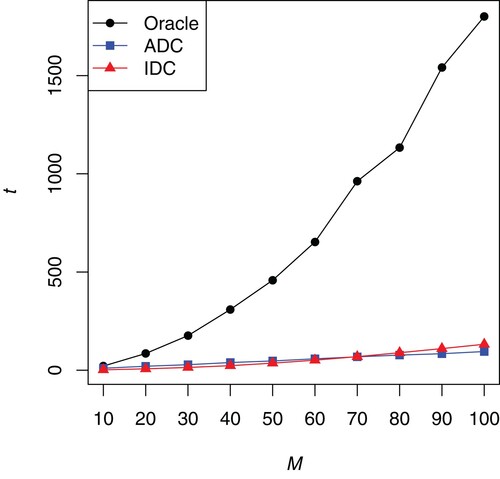
The results of MSE are presented in Figure 1. The average computing time in seconds used to estimate the index parameter is presented in Figure 1. From Figures 1 and 2, the following conclusions can be drawn.

1. From Figure 1, we can see that the performances of Oracle method are the best of the three methods under different M. However, by Figure 2, the operation times of Oracle method are much greater than those of ADC and IDC under different M.

2. As the number of blocks M continues to increase, the MSEs of Oracle and IDC decrease. However, ADC doesn't have this pattern.

3. If the number of blocks is less than 30, the MSEs of the ADC method are less than that of IDC. However, as the number of blocks continues to increase, IDC can significantly outperform the ADC method. Furthermore, if the number of blocks is less than 60, the operation times of the IDC method are less than that of ADC.

Figure 1. Comparison of MSE versus the number of blocks M with $\tilde{n}=100$ for three methods for simulation Example 3.2.

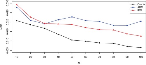
Figure 2. The mean computing time of $\hat{\mathit{\gamma }}$ (in seconds) for simulation Example 3.2.

3.3. Simulation example 3: effect of n

To examine the effect of increasing the sample size, n = 5000, 10000 and 20000 are considered. The following single-index model is considered: (9) $\mathbf{Y}=\sin \left(0.75{\mathbf{X}}^{\mathrm{\top }}{\mathit{\gamma }}_{01}\right)+\mathit{ϵ},$(9) where $\mathbf{X}=({\mathbf{X}}_1,{\mathbf{X}}_2{)}^{\mathrm{\top }}$ is a two-dimensional standard normal variable, the correlation between ${\mathbf{X}}_1$ and ${\mathbf{X}}_2$ is 0.5, ${\mathit{\gamma }}_{01}=(1,{\mathit{\gamma }}_0^{\mathrm{\top }}{)}^{\mathrm{\top }}$, ${\mathit{\gamma }}_0=2$ and $\mathit{ϵ}\sim N(0,{0.2}^2)$.

Table 2 presents the averages of Absolute Bias and computing time t over the 100 data sets along with its estimated standard error. By varying the sample size, as expected, the Absolute Bias becomes smaller and computing time t becomes bigger as the sample size grows.

Table 2. The means of Absolute Bias (standard deviation) and t for simulation Example 3.

		n = 5000		n = 10000		n = 20000
M	Methods	Absolute bias	t	Absolute bias	t	Absolute bias	t
1	Oracle	0.0083 (0.0042)	174	0.0048 (0.0036)	699	0.0043 (0.0032)	2628
10	ADC	0.0113 (0.0099)	22	0.0085 (0.0058)	76	0.0047 (0.0038)	287
	IDC	0.0239 (0.0015)	40	0.0118 (0.0090)	152	0.0051 (0.0044)	591
50	ADC	0.0731 (0.0571)	20	0.0140 (0.0092)	32	0.0051 (0.0027)	78
	IDC	0.0404 (0.0407)	53	0.0128 (0.0097)	178	0.0047 (0.0051)	640
100	ADC	0.1358 (0.0496)	34	0.0565 (0.0467)	41	0.0057 (0.0065)	62
	IDC	0.0893 (0.0293)	106	0.0347 (0.0259)	215	0.0051 (0.0060)	696

3.4. Real data example 1: combined cycle power plant data

We apply the proposed method to combined cycle power plant data. The dataset contains 9568 data points collected from a Combined Cycle Power Plant over 6 years (2006–2011), when the power plant was set to work with full load. Features consist of hourly average ambient variables Temperature (AT), Ambient Pressure (AP), Relative Humidity (RH) and Exhaust Vacuum (V) to predict the net hourly electrical energy output (EP) of the plant. The data set is obtained from online site: https://archive.ics.uci.edu/ml/datasets/Combined+Cycle+Power+Plant.

In this study, the following single-index model is used to fit the data: (10) $\mathrm{E}\mathrm{P}=g\{{\mathit{\gamma }}_1\mathrm{A}\mathrm{T}+{\mathit{\gamma }}_2\mathrm{A}\mathrm{P}+{\mathit{\gamma }}_3\mathrm{R}\mathrm{H}+{\mathit{\gamma }}_4\mathrm{V}\}+\mathit{ϵ},$(10) where all the data are normalized. We considered the number of blocks $M\in \{8,16,26,46,92\}$; hence, the respective values of the local sample size are $\tilde{n}\in \{1196,598,368,208,104\}$. Table 3 summarizes the estimated coefficients for the above model, showing that AP has the smallest effect on EP among the four covariates and AT is the most important covariate. Figure 3 shows the estimated EP by the Oracle method along with the observations, illustrating that single-index model (10(10) $\mathrm{E}\mathrm{P}=g\{{\mathit{\gamma }}_1\mathrm{A}\mathrm{T}+{\mathit{\gamma }}_2\mathrm{A}\mathrm{P}+{\mathit{\gamma }}_3\mathrm{R}\mathrm{H}+{\mathit{\gamma }}_4\mathrm{V}\}+\mathit{ϵ},$(10) ) is very suitable to the combined cycle power plant data. Furthermore, we evaluate the performances of three estimators based on mean square fitting error ($\mathrm{M}\mathrm{S}\mathrm{F}\mathrm{E}=\sum _{i=1}^{9568}|{\mathrm{E}\mathrm{P}}_i-{\widehat{\mathrm{E}\mathrm{P}}}_i|/9568$), where ${\widehat{\mathrm{E}\mathrm{P}}}_i$ is the fitted value of ${\mathrm{E}\mathrm{P}}_i$ by (3(3) $\hat{g}(u,\mathit{\gamma })=\frac{A_{2,0}(u,{\mathit{\gamma }}_1,h_1)A_{0,1}(u,{\mathit{\gamma }}_1,h_1)-A_{1,0}(u,{\mathit{\gamma }}_1,h_1)A_{1,1}(u,{\mathit{\gamma }}_1,h_1)}{A_{0,0}(u,{\mathit{\gamma }}_1,h_1)A_{2,0}(u,{\mathit{\gamma }}_1,h_1)-A_{1,0}^2(u,{\mathit{\gamma }}_1,h_1)},$(3) ). From Table 3, the following conclusions can be drawn.

1. The MSFEs of IDC under different M are very close to that of Oracle method. Thus the performances IDC are well.

2. As the number of blocks M continues to increase, the MSFEs of ADC increase. The performances of IDC estimator are better than those of ADC when M = 92 and are worse than those of ADC when M is small.

3. t in Table 3 is the average computing time in seconds used to estimate the index parameter. From t, we see that the operation times of IDC are faster than that of Oracle and ADC.

Figure 3. Estimated single index function for the combined cycle power plant data. The dots are the observations EP and the curve is the estimated EP by the Oracle method.

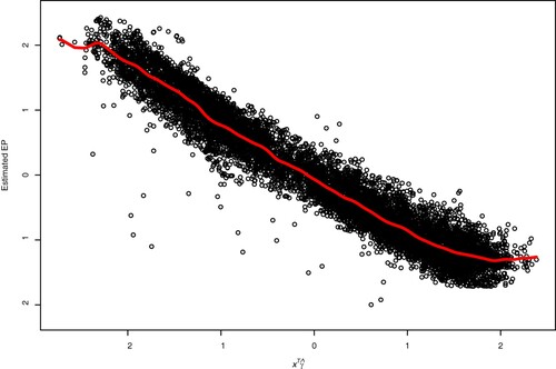
Table 3. The coefficient estimates and MSFE for the combined cycle power plant data.

M	Method	AT	AP	RH	V	MSFE	t
1	Oracle	1.0000	−0.0290	0.1326	0.2572	0.0627	4864
8	ADC	1.0000	−0.0287	0.1306	0.2670	0.0627	695
	IDC	1.0000	−0.0401	0.1348	0.2624	0.0628	229
16	ADC	1.0000	−0.0284	0.1299	0.2717	0.0627	395
	IDC	1.0000	−0.0346	0.1282	0.2657	0.0628	157
26	ADC	1.0000	−0.0267	0.1297	0.2727	0.0627	271
	IDC	1.0000	−0.0346	0.1282	0.2659	0.0628	154
46	ADC	1.0000	−0.0336	0.1256	0.2665	0.0628	222
	IDC	1.0000	−0.0345	0.1283	0.2654	0.0628	149
92	ADC	1.0000	−0.0391	0.1271	0.2702	0.0633	219
	IDC	1.0000	−0.0353	0.1275	0.2694	0.0628	145

3.5. Real data example 2: airline on-time data

Airline on-time performance data from the 2009 ASA Data Expo are used as a case study. These data are publicly available (http://stat-computing.org/dataexpo/2009/the-data.html). This dataset consists of flight arrival and departure details for all commercial flights within the United States from October 1987 to April 2008. About 12 million flights were recorded with 29 variables. In this section, we only consider the data of year 2008 (the number of samples is 1011963). The first 1000000 data points are used for the estimation and the remaining 11963 data are used for the prediction.

Schifano et al. (2016) developed a linear model that fits the data as follows: (11) $\mathrm{A}\mathrm{D}={\mathit{\gamma }}_1\mathrm{H}\mathrm{D}+{\mathit{\gamma }}_2\mathrm{D}\mathrm{I}\mathrm{S}+{\mathit{\gamma }}_3\mathrm{N}\mathrm{F}+{\mathit{\gamma }}_4\mathrm{W}\mathrm{F}+\mathit{ϵ},$(11) where $\mathrm{A}\mathrm{D}$ is the arrival delay (ArrDelay), which is a continuous variable found by modelling $\log (\mathrm{A}\mathrm{r}\mathrm{r}\mathrm{D}\mathrm{e}\mathrm{l}\mathrm{a}\mathrm{y}-min(\mathrm{A}\mathrm{r}\mathrm{r}\mathrm{D}\mathrm{e}\mathrm{l}\mathrm{a}\mathrm{y})+1)$, $\mathrm{H}\mathrm{D}$ is the departure hour (range 0 to 24), $\mathrm{D}\mathrm{I}\mathrm{S}$ is the distance (in 1000 miles), $\mathrm{N}\mathrm{F}$ is the dummy variable for a night flight (1 if departure between 8 p.m. and 5 a.m., 0 otherwise), and $\mathrm{W}\mathrm{F}$ is the dummy variable for a weekend flight (1 if departure occurred during the weekend, 0 otherwise).

In this study, the following single-index model is used to fit the data: (12) $\mathrm{A}\mathrm{D}=g\{{\mathit{\gamma }}_1\mathrm{H}\mathrm{D}+{\mathit{\gamma }}_2\mathrm{D}\mathrm{I}\mathrm{S}+{\mathit{\gamma }}_3\mathrm{N}\mathrm{F}+{\mathit{\gamma }}_4\mathrm{W}\mathrm{F}\}+\mathit{ϵ}.$(12) For comparison purposes, we use the least squares (LS) method to estimate $({\mathit{\gamma }}_1,{\mathit{\gamma }}_2,{\mathit{\gamma }}_3,{\mathit{\gamma }}_4{)}^{\mathrm{\top }}$ in model (11(11) $\mathrm{A}\mathrm{D}={\mathit{\gamma }}_1\mathrm{H}\mathrm{D}+{\mathit{\gamma }}_2\mathrm{D}\mathrm{I}\mathrm{S}+{\mathit{\gamma }}_3\mathrm{N}\mathrm{F}+{\mathit{\gamma }}_4\mathrm{W}\mathrm{F}+\mathit{ϵ},$(11) ), and use the ADC and IDC methods proposed in Section 2 to estimate $({\mathit{\gamma }}_1,{\mathit{\gamma }}_2,{\mathit{\gamma }}_3,{\mathit{\gamma }}_4{)}^{\mathrm{\top }}$ in model (12(12) $\mathrm{A}\mathrm{D}=g\{{\mathit{\gamma }}_1\mathrm{H}\mathrm{D}+{\mathit{\gamma }}_2\mathrm{D}\mathrm{I}\mathrm{S}+{\mathit{\gamma }}_3\mathrm{N}\mathrm{F}+{\mathit{\gamma }}_4\mathrm{W}\mathrm{F}\}+\mathit{ϵ}.$(12) ). The number of blocks is 1000 for these three methods. Furthermore, we evaluate the performance of these estimators based on their out-of-sample prediction with the mean absolute prediction error (MAPE) of the predictions, $\mathrm{M}\mathrm{A}\mathrm{P}\mathrm{E}=\frac{1}{n}\sum _{i=1}^n|{\mathrm{A}\mathrm{D}}_i-{\widehat{\mathrm{A}\mathrm{D}}}_i|,$where ${\widehat{\mathrm{A}\mathrm{D}}}_i$ is the fitted value of ${\mathrm{A}\mathrm{D}}_i$, $i=1,\dots ,n$ with n = 11, 963. ${\widehat{\mathrm{A}\mathrm{D}}}_i$ can be obtained by (3(3) $\hat{g}(u,\mathit{\gamma })=\frac{A_{2,0}(u,{\mathit{\gamma }}_1,h_1)A_{0,1}(u,{\mathit{\gamma }}_1,h_1)-A_{1,0}(u,{\mathit{\gamma }}_1,h_1)A_{1,1}(u,{\mathit{\gamma }}_1,h_1)}{A_{0,0}(u,{\mathit{\gamma }}_1,h_1)A_{2,0}(u,{\mathit{\gamma }}_1,h_1)-A_{1,0}^2(u,{\mathit{\gamma }}_1,h_1)},$(3) ). Table 4 presents the estimated coefficients and MAPEs of the three methods. From Table 4, we can see that the IDC method performs better than LS and ADC according to the smaller MAPE.

Table 4. The coefficient estimates and MAPE for the airline on-time data.

Method	HD	DIS	NF	WF	MAPE
LS	0.0044	−0.0505	−0.0004	−0.0451	0.2179
ADC	1.0000	−0.0271	0.0256	−0.0030	0.2051
IDC	1.0000	−0.0106	0.1216	−0.6948	0.2014

Disclosure statement

We proposed a divide-and-conquer method to deal with single-index model for massive dataset. The proposed method significantly reduces the required amount of primary memory and enjoys a very low computational cost. The proposed method achieves the same asymptotic efficiency as the estimator using all the data. Furthermore, it allows a weak condition on the sample size as a function of memory size.

Additional information

Funding

We would like to acknowledge support for this project from the Fundamental Research Funds for the Central Universities of China (No. 2232020D-43).

Appendix

Proof

Proof of Theorem 2.1

We denote the first iteration ${\hat{\mathit{\gamma }}}^1$, and note that (6(6) $\begin{array}{rl}\hat{\mathit{\gamma }}& =\arg \underset{\mathit{\gamma }}{min}\sum _{m=1}^M\sum _{i\in S_m}{\{Y_i-\hat{g}\left({\mathbf{X}}_i^{\mathrm{\top }}{\hat{\mathit{\gamma }}}_1^0\right)-{\hat{g}}^{\prime }\left({\mathbf{X}}_i^{\mathrm{\top }}{\hat{\mathit{\gamma }}}_1^0\right)({\mathbf{X}}_{i,-1}^{\mathrm{\top }}\mathit{\gamma }-{\mathbf{X}}_{i,-1}^{\mathrm{\top }}{\hat{\mathit{\gamma }}}^0)\}}^2\\ & ={\left\{\sum _{m=1}^M\sum _{i\in S_m}{\hat{g}}^{\prime 2}\left({\mathbf{X}}_i^{\mathrm{\top }}{\hat{\mathit{\gamma }}}_1^0\right){\mathbf{X}}_{i,-1}{\mathbf{X}}_{i,-1}^{\mathrm{\top }}\right\}}^{-1}\left\{\sum _{m=1}^M\sum _{i\in S_m}{\hat{g}}^{\prime }\left({\mathbf{X}}_i^{\mathrm{\top }}{\hat{\mathit{\gamma }}}_1^0\right){\mathbf{X}}_{i,-1}{Y}_i^{\ast }\right\},\end{array}$(6) ) can be equivalently written as ${\hat{\mathit{\gamma }}}^1-{\mathit{\gamma }}_0={\left\{\sum _{i=1}^n{\hat{g}}^{\prime 2}\left({\mathbf{X}}_i^{\mathrm{\top }}{\hat{\mathit{\gamma }}}_1^0\right){\mathbf{X}}_{i,-1}{\mathbf{X}}_{i,-1}^{\mathrm{\top }}\right\}}^{-1}\left\{\sum _{i=1}^n{\hat{g}}^{\prime }\left({\mathbf{X}}_i^{\mathrm{\top }}{\hat{\mathit{\gamma }}}_1^0\right){\mathbf{X}}_{i,-1}{\tilde{Y}}_i\right\}=U_n^{-1}{V}_n,$where ${\tilde{Y}}_i={ϵ}_i+g_0\left({\mathbf{X}}_i^{\mathrm{\top }}{\mathit{\gamma }}_{01}\right)-\hat{g}\left({\mathbf{X}}_i^{\mathrm{\top }}{\hat{\mathit{\gamma }}}_1^0\right)-{\hat{g}}^{\prime }\left({\mathbf{X}}_i^{\mathrm{\top }}{\hat{\mathit{\gamma }}}_1^0\right){\mathbf{X}}_{i,-1}^{\mathrm{\top }}({\mathit{\gamma }}_0-{\hat{\mathit{\gamma }}}^0)$, $V_n=n^{-1}\sum _{i=1}^n{\hat{g}}^{\prime }\left({\mathbf{X}}_i^{\mathrm{\top }}{\hat{\mathit{\gamma }}}_1^0\right){\mathbf{X}}_{i,-1}{\tilde{Y}}_i$, and $U_n=n^{-1}\times \sum _{i=1}^n{\hat{g}}^{\prime 2}\left({\mathbf{X}}_i^{\mathrm{\top }}{\hat{\mathit{\gamma }}}_1^0\right){\mathbf{X}}_{i,-1}{\mathbf{X}}_{i,-1}^{\mathrm{\top }}$. Note that $\begin{array}{rl}{V}_n& =\frac{1}{n}\sum _{i=1}^n{g}_0^{\prime }\left({\mathbf{X}}_i^{\mathrm{\top }}{\mathit{\gamma }}_{01}\right)\{{\mathbf{X}}_{i,-1}-E({\mathbf{X}}_{-1}\mid {\mathbf{X}}_i^{\mathrm{\top }}{\mathit{\gamma }}_{01})\}{ϵ}_i\\ & +\frac{1}{n}\sum _{i=1}^n\{{\hat{g}}^{\prime }\left({\mathbf{X}}_i^{\mathrm{\top }}{\hat{\mathit{\gamma }}}_1^0\right)-g_0^{\prime }\left({\mathbf{X}}_i^{\mathrm{\top }}{\mathit{\gamma }}_{01}\right)\}{\mathbf{X}}_{i,-1}{ϵ}_i\\ & +\frac{1}{n}\sum _{i=1}^n{g}_0^{\prime }\left({\mathbf{X}}_i^{\mathrm{\top }}{\mathit{\gamma }}_{01}\right)[{\mathbf{X}}_{i,-1}\{g_0\left({\mathbf{X}}_i^{\mathrm{\top }}{\mathit{\gamma }}_{01}\right)-\hat{g}\left({\mathbf{X}}_i^{\mathrm{\top }}{\mathit{\gamma }}_{01}\right)\}+E({\mathbf{X}}_{-1}\mid {\mathbf{X}}_i^{\mathrm{\top }}{\mathit{\gamma }}_{01}){ϵ}_i]\\ & +\frac{1}{n}\sum _{i=1}^n{\mathbf{X}}_{i,-1}\{{\hat{g}}^{\prime }\left({\mathbf{X}}_i^{\mathrm{\top }}{\hat{\mathit{\gamma }}}_1^0\right)-g_0^{\prime }\left({\mathbf{X}}_i^{\mathrm{\top }}{\mathit{\gamma }}_{01}\right)\}\{g_0\left({\mathbf{X}}_i^{\mathrm{\top }}{\mathit{\gamma }}_{01}\right)-\hat{g}\left({\mathbf{X}}_i^{\mathrm{\top }}{\mathit{\gamma }}_{01}\right)\}\\ & +\frac{1}{n}\sum _{i=1}^n{\hat{g}}^{\prime }\left({\mathbf{X}}_i^{\mathrm{\top }}{\hat{\mathit{\gamma }}}_1^0\right){\mathbf{X}}_{i,-1}\{\hat{g}\left({\mathbf{X}}_i^{\mathrm{\top }}{\mathit{\gamma }}_{01}\right)-\hat{g}\left({\mathbf{X}}_i^{\mathrm{\top }}{\hat{\mathit{\gamma }}}_1^0\right)-{\hat{g}}^{\prime }\left({\mathbf{X}}_i^{\mathrm{\top }}{\hat{\mathit{\gamma }}}_1^0\right){\mathbf{X}}_{i,-1}^{\mathrm{\top }}({\mathit{\gamma }}_0-{\hat{\mathit{\gamma }}}^0)\}\\ & \equiv V_{n1}+V_{n2}+V_{n3}+V_{n4}+V_{n5}.\end{array}$We first show that $\Vert V_{n2}{\Vert }_2=o_p\left(n^{-1/2}\right)$. Let $V_{n2,s}$ denote the s-th component of $V_{n2}$. Then, we have $\begin{array}{rl}{V}_{n2,s}& =\frac{1}{n}\sum _{i=1}^n\{{\hat{g}}^{\prime }\left({\mathbf{X}}_i^{\mathrm{\top }}{\hat{\mathit{\gamma }}}_1^0\right)-g_0^{\prime }\left({\mathbf{X}}_i^{\mathrm{\top }}{\mathit{\gamma }}_{01}\right)\}{\mathbf{X}}_{is,-1}{ϵ}_i\\ & =\frac{1}{n}\sum _{i=1}^n\{{\hat{g}}^{\prime }\left({\mathbf{X}}_i^{\mathrm{\top }}{\hat{\mathit{\gamma }}}_1^0\right)-g_0^{\prime }\left({\mathbf{X}}_i^{\mathrm{\top }}{\hat{\mathit{\gamma }}}_1^0\right)\}{\mathbf{X}}_{is,-1}{ϵ}_i\\ & +\frac{1}{n}\sum _{i=1}^n\{g_0^{\prime }\left({\mathbf{X}}_i^{\mathrm{\top }}{\hat{\mathit{\gamma }}}_1^0\right)-g_0^{\prime }\left({\mathbf{X}}_i^{\mathrm{\top }}{\mathit{\gamma }}_{01}\right)\}{\mathbf{X}}_{is,-1}{ϵ}_i\\ & \equiv V_{n21,s}+V_{n22,s}.\end{array}$Note that ${\hat{g}}^{\prime }(u,\mathit{\gamma })$ in (3(3) $\hat{g}(u,\mathit{\gamma })=\frac{A_{2,0}(u,{\mathit{\gamma }}_1,h_1)A_{0,1}(u,{\mathit{\gamma }}_1,h_1)-A_{1,0}(u,{\mathit{\gamma }}_1,h_1)A_{1,1}(u,{\mathit{\gamma }}_1,h_1)}{A_{0,0}(u,{\mathit{\gamma }}_1,h_1)A_{2,0}(u,{\mathit{\gamma }}_1,h_1)-A_{1,0}^2(u,{\mathit{\gamma }}_1,h_1)},$(3) ) can be rewritten as ${\hat{g}}^{\prime }(u,\mathit{\gamma })=\sum _{i=1}^n{\tilde{W}}_{ni}(u,{\mathit{\gamma }}_1)Y_i,$ where ${\tilde{W}}_{ni}(u,{\mathit{\gamma }}_1)=\frac{K_{h_2}({\mathbf{X}}_i^{\mathrm{\top }}{\mathit{\gamma }}_1-u)\left\{({\mathbf{X}}_i^{\mathrm{\top }}{\mathit{\gamma }}_1-u)A_{0,0}\right(u,{\mathit{\gamma }}_1,h_2)-A_{1,0}(u,{\mathit{\gamma }}_1,h_2\left)\right\}}{A_{0,0}(u,{\mathit{\gamma }}_1,h_2)A_{2,0}(u,{\mathit{\gamma }}_1,h_2)-A_{1,0}^2(u,{\mathit{\gamma }}_1,h_2)}.$Thus $V_{n21,s}$ can be rewritten as $\begin{array}{rl}{V}_{n21,s}& =\frac{1}{n}\sum _{i=1}^n\{\sum _{j=1}^n{\tilde{W}}_{nj}({\mathbf{X}}_i^{\mathrm{\top }}{\hat{\mathit{\gamma }}}_1^0,{\hat{\mathit{\gamma }}}_1^0)g_0\left({\mathbf{X}}_j^{\mathrm{\top }}{\hat{\mathit{\gamma }}}_1^0\right)-g_0^{\prime }\left({\mathbf{X}}_i^{\mathrm{\top }}{\hat{\mathit{\gamma }}}_1^0\right)\}{\mathbf{X}}_{is,-1}{ϵ}_i\\ & +\frac{1}{n}\sum _{i=1}^n{\tilde{W}}_{ni}({\mathbf{X}}_i^{\mathrm{\top }}{\hat{\mathit{\gamma }}}_1^0,{\hat{\mathit{\gamma }}}_1^0){\mathbf{X}}_{is,-1}{ϵ}_i^2+\frac{1}{n}\sum _{i=2}^n\sum _{j=1}^{i-1}{a}_{ij}{ϵ}_j{ϵ}_i\\ & \equiv V_{n211,s}+V_{n212,s}+V_{n213,s},\end{array}$where $a_{ij}={\tilde{W}}_{nj}\left({\mathbf{X}}_i^{\mathrm{\top }}{\hat{\mathit{\gamma }}}_1^0\right){\mathbf{X}}_{is,-1}+{\tilde{W}}_{ni}\left({\mathbf{X}}_j^{\mathrm{\top }}{\hat{\mathit{\gamma }}}_1^0\right){\mathbf{X}}_{js,-1}.$Hence, by Lemma 1 in Zhu and Xue (2006) and conditions (C2) and (C3), ${\hat{\mathit{\gamma }}}^0$ is a consistent estimate of ${\mathit{\gamma }}_0$ and by the Cauchy–Schwarz inequality, for $c_1$ and $c_2$ big enough, we have $\begin{array}{rl}nE\left[V_{n211,s}^2\right]& =\frac{1}{n}\sum _{i=1}^{n}E\left[{\{\sum _{j=1}^n{\tilde{W}}_{nj}({\mathbf{X}}_i^{\mathrm{\top }}{\hat{\mathit{\gamma }}}_1^0,{\hat{\mathit{\gamma }}}_1^0)g_0({\mathbf{X}}_j^{\mathrm{\top }},{\hat{\mathit{\gamma }}}_1^0)-g_0^{\prime }\left({\mathbf{X}}_i^{\mathrm{\top }}{\hat{\mathit{\gamma }}}_1^0\right)\}}^2{\mathbf{X}}_{is,-1}^{2}E\right({ϵ}_i^2\mid {\mathbf{X}}_i\left)\right]\\ & \le c_1\frac{1}{n}\sum _{i=1}^n{\left[E{\{\sum _{j=1}^n{\tilde{W}}_{nj}({\mathbf{X}}_i^{\mathrm{\top }}{\hat{\mathit{\gamma }}}_1^0,{\hat{\mathit{\gamma }}}_1^0)g_0\left({\mathbf{X}}_j^{\mathrm{\top }}{\hat{\mathit{\gamma }}}_1^0\right)-g_0^{\prime }\left({\mathbf{X}}_i^{\mathrm{\top }}{\hat{\mathit{\gamma }}}_1^0\right)\}}^4\right]}^{1/2}\left\{E\right({\mathbf{X}}_{is,-1}{)}^4{\}}^{1/2}\\ & \le c_2{h}_2^2\to 0.\end{array}$For $V_{n212,s}$, by Lemma 2 in Zhu and Xue (2006), for $c_3$ and $c_4$ big enough, we have $\begin{array}{rl}\sqrt{n}E|V_{n212,s}|& \le \frac{1}{\sqrt{n}}\sum _{i=1}^{n}E\left\{\left|{\tilde{W}}_{ni}({\mathbf{X}}_i^{\mathrm{\top }}{\hat{\mathit{\gamma }}}_1^0,{\hat{\mathit{\gamma }}}_1^0){\mathbf{X}}_{is,-1}\right|E\right({ϵ}_i^2\mid {\mathbf{X}}_i\left)\right\}\\ & \le c_3\frac{1}{\sqrt{n}}\sum _{i=1}^n\sqrt{E{\left\{{\tilde{W}}_{nj}({\mathbf{X}}_i^{\mathrm{\top }}{\hat{\mathit{\gamma }}}_1^0,{\hat{\mathit{\gamma }}}_1^0)\right\}}^2}\sqrt{E\left({\mathbf{X}}_{is,-1}^2\right)}\\ & \le c_4\left\{\right(n{h}_2^2{)}^{-1/2}+\left(n{h}_2^{5/2}{)}^{-1}\right\}\to 0.\end{array}$We now consider $V_{n213,s}$. Note that $E(a_{ij}{ϵ}_j{ϵ}_i\mid X,{ϵ}_j)=0$ and $E(a_{i_1{j}_1}{ϵ}_{j_1}{ϵ}_{i_1}{a}_{i_2{j}_2}{ϵ}_{j_2}{ϵ}_{i_2}\mid X)=0$ when $\{i_1,j_1\}\ne \{i_2,j_2\}$; by Lemma 2 in Zhu and Xue (2006), for $c_5$ and $c_6$ big enough, we have $\begin{array}{rl}nE\left(V_{n213,s}^2\right)& =\frac{1}{n}\sum _{i=2}^n\sum _{j=1}^{i-1}E\left\{a_{ij}^{2}E\right({ϵ}_j^2\mid {\mathbf{X}}_{js}\left)E\right({ϵ}_i^2\mid {\mathbf{X}}_{is}\left)\right\}\\ & \le c_5\frac{1}{n}\sum _{i\ne j}\sqrt{E{\left\{{\tilde{W}}_{nj}({\mathbf{X}}_i^{\mathrm{\top }}{\hat{\mathit{\gamma }}}_1^0,{\hat{\mathit{\gamma }}}_1^0)\right\}}^4}\sqrt{E\left({\mathbf{X}}_{is,-1}^4\right)}\\ & \le c_6\left\{\right(n_2{h}_2^3{)}^{-1}+n^{-1}\sqrt{h_2}+\left(n{h}_2^{5/2}{)}^{-2}\right\}\to 0.\end{array}$By the condition $\Vert {\hat{\mathit{\gamma }}}^0-{\mathit{\gamma }}_0{\Vert }_2=O_p\left({\tilde{n}}^{-1/2}\right)$, we have $V_{n22,s}=o_p\left(n^{-1/2}\right).$ Combining the above results, the s-th moment of $V_{n2}$ converges to 0. By the Markov inequality, we have $\Vert V_{n2}{\Vert }_2=o_p\left(n^{-1/2}\right).$We prove that the mean and the variance of $n^{1/2}{V}_{n3,s}$ tend to 0. Using $E\{\hat{g}\left({\mathbf{X}}_i^{\mathrm{\top }}{\mathit{\gamma }}_{01}\right)-g_0\left({\mathbf{X}}_i^{\mathrm{\top }}{\mathit{\gamma }}_{01}\right)\}=O\left(h_1^2\right)$and condition (C2), we have $\sqrt{n}E{V}_{n3,s}\le O\left(n^{1/2}{h}_1^2\right)\to 0.$Using conditions (C1)–(C4) and the (A.35) of Chang et al. (2010), we obtain $nE{V}_{n3,s}^2\le O(n{h}_1^4+\sqrt{h_1}+(n{h}_1{)}^{-1})\to 0.$This proves that $\Vert V_{n3}{\Vert }_2=o_p\left(n^{-1/2}\right).$We now consider $V_{n4}$. $\begin{array}{rl}{V}_{n4,s}& =\frac{1}{n}\sum _{i=1}^n{\mathbf{X}}_{is,-1}\{{\hat{g}}^{\prime }\left({\mathbf{X}}_i^{\mathrm{\top }}{\hat{\mathit{\gamma }}}_1^0\right)-g_0^{\prime }\left({\mathbf{X}}_i^{\mathrm{\top }}{\hat{\mathit{\gamma }}}_1^0\right)\}\{g_0\left({\mathbf{X}}_i^{\mathrm{\top }}{\mathit{\gamma }}_{01}\right)-\hat{g}\left({\mathbf{X}}_i^{\mathrm{\top }}{\mathit{\gamma }}_{01}\right)\}\\ & +\frac{1}{n}\sum _{i=1}^n{\mathbf{X}}_{is,-1}\{g_0^{\prime }\left({\mathbf{X}}_i^{\mathrm{\top }}{\hat{\mathit{\gamma }}}_1^0\right)-g_0^{\prime }\left({\mathbf{X}}_i^{\mathrm{\top }}{\mathit{\gamma }}_{01}\right)\}\{g_0\left({\mathbf{X}}_i^{\mathrm{\top }}{\mathit{\gamma }}_{01}\right)-\hat{g}\left({\mathbf{X}}_i^{\mathrm{\top }}{\mathit{\gamma }}_{01}\right)\}\\ & \equiv V_{n41,s}+V_{n42,s}.\end{array}$By Lemma 3 in Zhu and Xue (2006) and Markov inequality, for any $ϵ>0$, $\begin{array}{rl}& P(\sqrt{\frac{n{h}_2^3}{\log n}}|{\hat{g}}^{\prime }\left({\mathbf{X}}_i^{\mathrm{\top }}{\hat{\mathit{\gamma }}}_1^0\right)-g_0^{\prime }\left({\mathbf{X}}_i^{\mathrm{\top }}{\hat{\mathit{\gamma }}}_1^0\right)|\ge ϵ)\\ & \le \frac{n{h}_2^3}{\log n}E{\{{\hat{g}}^{\prime }\left({\mathbf{X}}_i^{\mathrm{\top }}{\hat{\mathit{\gamma }}}_1^0\right)-g_0^{\prime }\left({\mathbf{X}}_i^{\mathrm{\top }}{\hat{\mathit{\gamma }}}_1^0\right)\}}^2/{ϵ}^2\to 0.\end{array}$Hence, we have, uniformly over $1\le i\le n$, $|{\hat{g}}^{\prime }\left({\mathbf{X}}_i^{\mathrm{\top }}{\hat{\mathit{\gamma }}}_1^0\right)-g_0^{\prime }\left({\mathbf{X}}_i^{\mathrm{\top }}{\hat{\mathit{\gamma }}}_1^0\right)|=O_p\left(\sqrt{\frac{\log n}{n{h}_2^3}}\right).$Similarly, $|\hat{g}\left({\mathbf{X}}_i^{\mathrm{\top }}{\hat{\mathit{\gamma }}}_1^0\right)-g_0\left({\mathbf{X}}_i^{\mathrm{\top }}{\hat{\mathit{\gamma }}}_1^0\right)|=O_p\left(\sqrt{\frac{\log n}{n{h}_1}}\right).$Thus we have $\begin{array}{rl}\sqrt{n}|V_{n41,s}|& \le \frac{1}{\sqrt{n}}\sum _{i=1}^n|{\mathbf{X}}_{is,-1}||{\hat{g}}^{\prime }\left({\mathbf{X}}_i^{\mathrm{\top }}{\hat{\mathit{\gamma }}}_1^0\right)-g_0^{\prime }\left({\mathbf{X}}_i^{\mathrm{\top }}{\hat{\mathit{\gamma }}}_1^0\right)||g_0\left({\mathbf{X}}_i^{\mathrm{\top }}{\mathit{\gamma }}_{01}\right)-\hat{g}\left({\mathbf{X}}_i^{\mathrm{\top }}{\mathit{\gamma }}_{01}\right)|\\ & =O_p\left(\sqrt{\frac{{\log }^{2}n}{n{h}_1{h}_2^3}}\right).\end{array}$Noting that $n{h}_1{h}_2^3/{\log }^{2}n\to \mathrm{\infty }$, we obtain $V_{n41,s}=o_p\left(n^{-1/2}\right).$ For $V_{n42}$, by a Taylor expansion, we get $V_{n42,s}=\frac{1}{n}\sum _{i=1}^n{g}^{″}\left({\xi }_i\right){\mathbf{X}}_{is,-1}{\mathbf{X}}_i^{\mathrm{\top }}({\hat{\mathit{\gamma }}}_1^0-{\mathit{\gamma }}_{01})\{g_0\left({\mathbf{X}}_i^{\mathrm{\top }}{\mathit{\gamma }}_{01}\right)-\hat{g}\left({\mathbf{X}}_i^{\mathrm{\top }}{\mathit{\gamma }}_{01}\right)\},$where ${\xi }_i$ is a point between ${\mathbf{X}}_i^{\mathrm{\top }}{\mathit{\gamma }}_{01}$ and ${\mathbf{X}}_i^{\mathrm{\top }}{\hat{\mathit{\gamma }}}_1^0$. By the condition $\Vert {\hat{\mathit{\gamma }}}^0-{\mathit{\gamma }}_0{\Vert }_2=O_p\left({\tilde{n}}^{-1/2}\right)$ and using $E\{\hat{g}\left({\mathbf{X}}_i^{\mathrm{\top }}{\mathit{\gamma }}_{01}\right)-g_0\left({\mathbf{X}}_i^{\mathrm{\top }}{\mathit{\gamma }}_{01}\right)\}=O\left(h_1^2\right)$, we have $\sqrt{n}E{V}_{n42,s}=O\left({\tilde{n}}^{-1/2}\sqrt{n}{h}_1^2\right)\to 0,$and $nE{V}_{n42,s}^2\le O(h_1^4{\tilde{n}}^{-1}+(\tilde{n}n{h}_1{)}^{-1})\to 0.$Thus we can obtain $V_{n42,s}=o_p\left(n^{-1/2}\right)$. Therefore, $\Vert V_{n4}{\Vert }_2=o_p\left(n^{-1/2}\right).$Finally, we consider $V_{n5}$. $V_{n5,s}=V_{n51,s}+V_{n52,s},$where $V_{n51,s}=n^{-1}\sum _{i=1}^n{g}_0^{\prime }\left({\mathbf{X}}_i^{\mathrm{\top }}{\hat{\mathit{\gamma }}}_1^0\right){\mathbf{X}}_{is,-1}\{\hat{g}\left({\mathbf{X}}_i^{\mathrm{\top }}{\mathit{\gamma }}_{01}\right)-\hat{g}\left({\mathbf{X}}_i^{\mathrm{\top }}{\hat{\mathit{\gamma }}}_1^0\right)-{\hat{g}}^{\prime }\left({\mathbf{X}}_i^{\mathrm{\top }}{\hat{\mathit{\gamma }}}_1^0\right){\mathbf{X}}_{i,-1}^{\mathrm{\top }}({\mathit{\gamma }}_0-{\hat{\mathit{\gamma }}}^0)\}$and $V_{n52,s}=n^{-1}\sum _{i=1}^n\{{\hat{g}}^{\prime }\left({\mathbf{X}}_i^{\mathrm{\top }}{\hat{\mathit{\gamma }}}_1^0\right)-g_0^{\prime }\left({\mathbf{X}}_i^{\mathrm{\top }}{\hat{\mathit{\gamma }}}_1^0\right)\}{\mathbf{X}}_{is,-1}\{\hat{g}\left({\mathbf{X}}_i^{\mathrm{\top }}{\mathit{\gamma }}_{01}\right)-\hat{g}\left({\mathbf{X}}_i^{\mathrm{\top }}{\hat{\mathit{\gamma }}}_1^0\right)-{\hat{g}}^{\prime }\left({\mathbf{X}}_i^{\mathrm{\top }}{\hat{\mathit{\gamma }}}_1^0\right){\mathbf{X}}_{i,-1}^{\mathrm{\top }}({\mathit{\gamma }}_0-{\hat{\mathit{\gamma }}}^0)\}.$We rewrite $V_{n51,s}$ as $\begin{array}{rl}{V}_{n51,s}& =\frac{1}{n}\sum _{i=1}^n{g}_0^{\prime }\left({\mathbf{X}}_i^{\mathrm{\top }}{\hat{\mathit{\gamma }}}_1^0\right){\mathbf{X}}_{is,-1}\{g_0\left({\mathbf{X}}_i^{\mathrm{\top }}{\mathit{\gamma }}_{01}\right)-g_0\left({\mathbf{X}}_i^{\mathrm{\top }}{\hat{\mathit{\gamma }}}_1^0\right)-g_0^{\prime }\left({\mathbf{X}}_i^{\mathrm{\top }}{\hat{\mathit{\gamma }}}_1^0\right){\mathbf{X}}_{i,-1}^{\mathrm{\top }}({\mathit{\gamma }}_0-{\hat{\mathit{\gamma }}}^0)\}\\ & +\frac{1}{n}\sum _{i=1}^n{g}_0^{\prime }\left({\mathbf{X}}_i^{\mathrm{\top }}{\hat{\mathit{\gamma }}}_1^0\right){\mathbf{X}}_{is,-1}\{\hat{g}\left({\mathbf{X}}_i^{\mathrm{\top }}{\mathit{\gamma }}_{01}\right)-g_0\left({\mathbf{X}}_i^{\mathrm{\top }}{\mathit{\gamma }}_{01}\right)\}\\ & -\frac{1}{n}\sum _{i=1}^n{g}_0^{\prime }\left({\mathbf{X}}_i^{\mathrm{\top }}{\hat{\mathit{\gamma }}}_1^0\right){\mathbf{X}}_{is,-1}\{\hat{g}\left({\mathbf{X}}_i^{\mathrm{\top }}{\hat{\mathit{\gamma }}}_1^0\right)-g_0\left({\mathbf{X}}_i^{\mathrm{\top }}{\hat{\mathit{\gamma }}}_1^0\right)\}\\ & -\frac{1}{n}\sum _{i=1}^n{g}_0^{\prime }\left({\mathbf{X}}_i^{\mathrm{\top }}{\hat{\mathit{\gamma }}}_1^0\right){\mathbf{X}}_{is,-1}\{{\hat{g}}^{\prime }\left({\mathbf{X}}_i^{\mathrm{\top }}{\hat{\mathit{\gamma }}}_1^0\right)-g_0^{\prime }\left({\mathbf{X}}_i^{\mathrm{\top }}{\hat{\mathit{\gamma }}}_1^0\right)\}{\mathbf{X}}_{i,-1}^{\mathrm{\top }}({\mathit{\gamma }}_0-{\hat{\mathit{\gamma }}}^0)\\ & \equiv V_{n511,s}+V_{n512,s}+V_{n513,s}+V_{n514,s}.\end{array}$For $V_{n511,s}$, by a Taylor expansion, we get $V_{n511}=O_p\left({\tilde{n}}^{-1}\right)$. Similar to the proof of $V_{n42,s}$, we get $\begin{array}{rl}& \sqrt{n}E{V}_{n512,s}=\sqrt{n}E{V}_{n513,s}=O\left(\sqrt{n}{h}_1^2\right)\to 0,\\ & nE{V}_{n512,s}^2=nE{V}_{n513,s}^2=O(h_1^4+(n{h}_1{)}^{-1})\to 0,\end{array}$and $\sqrt{n}E{V}_{n514,s}=O\left(\sqrt{n/\tilde{n}}{h}_2^2\right)\to 0,nE{V}_{n514,s}^2=O({\tilde{n}}^{-1}{h}_2^2+{\tilde{n}}^{-1}{n}^{-1}{h}_2^{-3})\to 0.$Hence, $\Vert V_{n5}{\Vert }_2=o_p\left(n^{-1/2}\right)+O_p\left({\tilde{n}}^{-1}\right).$Therefore, we have $V_n=\frac{1}{n}\sum _{i=1}^n{g}_0^{\prime }\left({\mathbf{X}}_i^{\mathrm{\top }}{\mathit{\gamma }}_{01}\right)\{{\mathbf{X}}_{i,-1}-E({\mathbf{X}}_{-1}\mid {\mathbf{X}}_i^{\mathrm{\top }}{\mathit{\gamma }}_{01})\}{ϵ}_i+o_p\left(n^{-1/2}\right)+O_p\left({\tilde{n}}^{-1}\right).$Similar to the proof of $V_n$, we can obtain $U_n=\mathbf{\Sigma }+o_p\left(1\right),$ where $\mathbf{\Sigma }=E\left\{g_0^{\prime 2}\left({\mathbf{X}}^{\mathrm{\top }}{\mathit{\gamma }}_{01}\right){\mathbf{X}}_{-1}{\mathbf{X}}_{-1}^{\mathrm{\top }}\right\}$. Thus ${\hat{\mathit{\gamma }}}^1-{\mathit{\gamma }}_0={\mathbf{\Sigma }}^{-1}\frac{1}{n}\sum _{i=1}^n{g}_0^{\prime }\left({\mathbf{X}}_i^{\mathrm{\top }}{\mathit{\gamma }}_{01}\right)\{{\mathbf{X}}_{i,-1}-E({\mathbf{X}}_{-1}\mid {\mathbf{X}}_i^{\mathrm{\top }}{\mathit{\gamma }}_{01})\}{ϵ}_i+o_p\left(n^{-1/2}\right)+O_p\left({\tilde{n}}^{-1}\right).$Note that one round of aggregation enables a refinement of the estimator with its bias reducing from ${\tilde{n}}^{-1/2}$ to ${\tilde{n}}^{-1}$. Therefore, an iterative refinement of the initial estimator will successively improve the estimation accuracy. The q-th iterative divide-and-conquer method ${\hat{\mathit{\gamma }}}^q$ satisfies $\begin{array}{rl}{\hat{\mathit{\gamma }}}^q-{\mathit{\gamma }}_0& ={\mathbf{\Sigma }}^{-1}\frac{1}{n}\sum _{i=1}^n{g}_0^{\prime }\left({\mathbf{X}}_i^{\mathrm{\top }}{\mathit{\gamma }}_{01}\right)\{{\mathbf{X}}_{i,-1}-E({\mathbf{X}}_{-1}\mid {\mathbf{X}}_i^{\mathrm{\top }}{\mathit{\gamma }}_{01})\}{ϵ}_i\\ & +o_p\left(n^{-1/2}\right)+O_p\left({\tilde{n}}^{-2^{q-1}}\right).\end{array}$Thus, after Q iterations, where $Q\ge 1+\log (\log n/\log \tilde{n})/\log 2$, we have $\hat{\mathit{\gamma }}-{\mathit{\gamma }}_0={\mathbf{\Sigma }}^{-1}\frac{1}{n}\sum _{i=1}^n{g}_0^{\prime }\left({\mathbf{X}}_i^{\mathrm{\top }}{\mathit{\gamma }}_{01}\right)\{{\mathbf{X}}_{i,-1}-E({\mathbf{X}}_{-1}\mid {\mathbf{X}}_i^{\mathrm{\top }}{\mathit{\gamma }}_{01})\}{ϵ}_i+o_p\left(n^{-1/2}\right).$By the central limit theorem, we can prove Theorem 2.1.

References

- Chen, X., Liu, W., & Zhang, Y. (2019). Quantile regression under memory constraint. The Annals of Statistics, 47(6), 3244–3273. https://doi.org/10.1214/18-AOS1777
- Chen, X. Y., & Xie, M. G. (2014). A split-and-conquer approach for analysis of extraordinarily large data. Statistica Sinica, 24(4), 1655–1684. https://doi.org/10.5705/ss.2013.088
- Christou, E., & Akritas, M. (2016). Single index quantile regression for heteroscedastic data. Journal of Multivariate Analysis, 150, 169–182. https://doi.org/10.1016/j.jmva.2016.05.010
- Delecroix, M., Hristache, M., & Patilea, V. (2006). On semiparametric M-estimation in single-index regression. Journal of Statistical Planning and Inference, 136(3), 730–769. https://doi.org/10.1016/j.jspi.2004.09.006
- Ichimura, H. (1993). Semiparametric least squares (SLS) and weighted SLS estimation of single-index models. Journal of Econometrics, 58(1-2), 71–120. https://doi.org/10.1016/0304-4076(93)90114-K
- Jiang, R., Guo, M. F., & Liu, X. (2020). Composite quasi-likelihood for single-index models with massive datasets. Communications in Statistics – Simulation and Computation, 51(9), 5024–5040. https://doi.org/10.1080/03610918.2020.1753074
- Jiang, R., Qian, W. M., & Zhou, Z. G. (2016). Weighted composite quantile regression for single-index models. Journal of Multivariate Analysis, 148, 34–48. https://doi.org/10.1016/j.jmva.2016.02.015
- Jiang, R., Zhou, Z. G., Qian, W. M., & Chen, Y. (2013). Two step composite quantile regression for single-index models. Computational Statistics & Data Analysis, 64, 180–191. https://doi.org/10.1016/j.csda.2013.03.014
- Jordan, M., Lee, J., & Yang, Y. (2019). Communication-efficient distributed statistical learning. Journal of the American Statistical Association, 14(526), 668–681. https://doi.org/10.1080/01621459.2018.1429274
- Lin, N., & Xi, R. (2011). Aggregated estimating equation estimation. Statistics and Its Interface, 4(1), 73–83. https://doi.org/10.4310/SII.2011.v4.n1.a8
- Schifano, E., Wu, J., Wang, C., Yan, J., & Chen, M. H. (2016). Online updating of statistical inference in the big data setting. Technometrics, 58(3), 393–403. https://doi.org/10.1080/00401706.2016.1142900
- Tang, Y., Wang, H., & Liang, H. (2018). Composite estimation for single-index models with responses subject to detection limits. Scandinavian Journal of Statistics, 45(3), 444–464. https://doi.org/10.1111/sjos.v45.3
- Wang, J. L., Xue, L., Zhu, L., & Chong, Y. (2010). Estimation for a partial-linear single-index model. The Annals of Statistics, 38(1), 246–274. https://doi.org/10.1214/09-AOS712
- Wu, T., Yu, K., & Yu, Y. (2010). Single-index quantile regression. Journal of Multivariate Analysis, 101(7), 1607–1621. https://doi.org/10.1016/j.jmva.2010.02.003
- Xia, Y., Tong, H., Li, W., & Zhu, L. X. (2002). An adaptive estimation of dimension reduction space. Journal of the Royal Statistical Society Series B, 64(3), 363–410. https://doi.org/10.1111/rssb.2002.64.issue-3
- Zhu, L., & Xue, L. (2006). Empirical likelihood confidence regions in a partially linear single-index model. Journal of the Royal Statistical Society: Series B, 68(3), 549–570. https://doi.org/10.1111/rssb.2006.68.issue-3