Application of neural network to model rainfall pattern of Ethiopia

Abstract

In this paper, we have constructed Artificial Neural Network models which could capture rainfall pattern of Ethiopia. The data was collected from 147 stations across Ethiopia. Seven homogenized rainfall stations have been created based on both local and global patterns of datasets. Back-of-Word algorithm was used for extracting patterns of the datasets. K-means algorithm was used for clustering purpose. Each of the data of homogenized regions was interpolated using a spatial average. Two time series models, ARMA and Facebook's Prophet, have been fitted for each of spatial averages as baseline models. Both have been shown to perform weak for generalization purpose as spatially averaged datasets lose their strong seasonal pattern. On the other hand, the proposed Long Short Term Memory (LSTM) was found to be the best fitted model in comparison to the baseline models. The hyperparameters of the LSTM have been tuned to get optimal parameters. Besides, the RMSE of the baseline model was used as a benchmark for tuning the LSTM used.

Keywords:

• ARIMA
• Back-of-Word algorithm
• clustering
• neural network
• Prophet

1. Introduction

Most Ethiopians depend on farming which is directly or indirectly related to precipitations. On the other hand, Ethiopia has a complex topography and a diversified climate (Berhanu et al., 2014). This leads to variation in rainfall amount among different geographical regions in this country.

Knowledge of near future pattern of the rainfall has a great impact on farming and hence plays a crucial role in the economy of the country. So accuracy in the prediction is very important. To get more guarantee in the forecasting, we need better predictive models.

By aggregating the datasets, one could generate a univariate dataset which could centre the datasets. A mathematical formula used for spatial averaging for aggregation purposes is well defined in Shen (2017) where it was shown that averaging approach works well for climate data. On the other hand, some authors have relied on a grid rainfall data to construct homogeneous rainfall regions. For example, Tsidu (2012) worked on homogenization, reconstruction and gridding onto a regular 0.5 by 0.5 resolution grid for data obtained from Ethiopia.

Besides these works, modelling time series data and forecasting their near future patterns has been a major research topic in time series analysis. In the historical development of this area, simple forecast methods, such as moving average, have been widely applied, especially when the data exhibits a smoothness rather than strong cyclically.

Since time series data are sequential in their nature, recurrent neural network can best describe this kind of data structure. To capture long-term pattern of the data, long-short-term memory architecture (LSTM) was designed by Hochreiter and Schmidhuber (1997), which is a variant of the recurrent neural network.

A better architecture of LSTMs leads to having a better ability to fit the data in hand and also the architecture works well for prediction purposes. By this, the LSTM was found to be a competitive model for seasonal data, like rainfall. Brownlee (2016) gave a good insight into how to handle the algorithm. In an earlier time, Facebook's Core Data Science team prepared a model called Prophet (Taylor & Letham, 2018a). This model, in its design, was intended to capture seasonal structure. So, Prophet was also found to be a competitive model for seasonal data. The prediction power of LSTM versus Facebook's Prophet model and the traditional time series model, ARIMA has been investigated using a number of time series data by a number of researchers. Strauß (2018) compared Prophet and LSTM models. Dabakoglu (2019) and Jiang and Zhang (2018) compared all the three models. Abbot and Marohasy (2018) constructed a predictive Artificial Neural Network (ANN) model of monthly rainfall for different locations in southeastern Queensland, Australia. They have compared the predictive power of this architecture against Predictive Ocean-Atmosphere Model for Australia (POAMA) and Climatology models.

The main objective of this study is to apply artificial neural network models to model the pattern of rainfall data. Since LSTM seems to be more flexible than other seasonal models, we used it for modelling purposes. We are interested in architecture which is simple and able to forecast with minimum errors.

2. Data and methods

2.1. Data source

On the basis of their spatial distribution and time lags the rainfall data of selected stations were taken from the National Methodology Agency of Ethiopia. A total of 147 rainfall stations have been considered at the data cleaning stage. Figure 1 shows the spatial distribution of the rainfall stations.

Figure 1. Spatial distribution of rainfall stations.

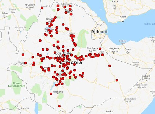
The maximum length for the duration of the data record is over January 1987 to April 2018.

2.2. Data cleaning

Before running into the model construction, we need to fix for missing values and outliers found in the data. Besides, we need to cluster rainfall stations having the same patterns.

2.2.1. Treating missing values

There are a number of approaches to estimate missing values. For climate data, Longley et al. (2005) suggested the inverse distance weighted spatial interpolation method.

The Inverse distance weighted interpolation methods intend to give differential weights to observations based on their proximity to the missing value (Haining & Haining, 2003). Distance weighting is introduced to capture the idea that attribute values close in distance tend to be similar but that the similarity weakens as distance separation increases. So it is the nearest site that should be given the most weight in the imputation.

In both clustering and estimation, only stations having at most 10% missing values were used. But we do not discard the data from stations having more than 10% missing values completely in our work, as we use them while imputation. The distances between stations were computed based on their geographical locations (i.e., latitude and longitude). This task has been handled by the geosphere package in R, using the mdist function (Hijmans, 2017).

2.2.2. Treating outliers

Detection of outliers has been done for each station independently which passes the selection criteria based on the size of missing value earlier to the treatment of missing values.

For detection and imputation of outliers, we have used the fpp package in R developed by Hyndman (2013) following the work of Chen and Liu (1993). They proposed an iterative outlier detection and estimation method for seasonal and non-seasonal ARMA processes to get joint estimates of model parameters and outlier effects.

2.3. Clustering and centring datasets

To cluster rainfall stations having similar pattern and homogenize rainfall stations, we applied the usual k-means algorithm to the transformed data rather than to the original data sets.

Data are transformed using a symbolic aggregated approximation (SAX) approach based on a normalized version of the data and further the data reduced by the dimensional reduction tool called piecewise aggregated approximation (PAA). Finally SAX was used to make the data set have discrete nature (Lin & Li, 2009).

For a time series of length n, PAA reduces the dimensionality of the data into a user-defined number, w (w<n) of equal length. Then the value of PAA values is transformed into symbols by using a breakpoint table generated by the regions having approximately equiprobability based on Gaussian distribution. This is easily achieved since normalized time series have a Gaussian distribution (Lonardi & Patel, 2002). In this case, we need an additional parameter which is the alphabet size, α ($\alpha >2$). And the data is needed to be transformed to have mean zero and variance one.

A time series C of length n, i.e., $C=c_1,c_2,\dots ,c_n$ can be represented by w dimensional space of vector $\overline{C}={\overline{c}}_1,{\overline{c}}_2,\dots ,{\overline{c}}_w$. The ${\overline{c}}_i$ are calculated as follows Lin et al. (2007): ${\overline{c}}_i=\frac{w}{n}\sum _{j=\frac{n}{w}(i-1)+1}^{\frac{n}{w}i}{c}_j.$ Then we need the PAA approximation $\overline{C}$ to be mapped to a word $\hat{C}$ as follows: ${\hat{c}}_i={\alpha }_i\mathrm{i}\mathrm{f}\mathrm{f}{\text{β}}_{j-1}\le {\overline{c}}_j\le {\text{β}}_j,$ where ${\text{β}}_j$ denotes the j-th breakpoint and ${\alpha }_1=a$, ${\alpha }_2=b$, ${\alpha }_3=c$, …. This process of mapping is called Symbolic Aggregate approXimation (SAX). The breakpoint is computed as ${\text{β}}_j={\mathrm{\Phi }}_X^{-1}\left(\frac{j}{\alpha }\right)$ where $X\sim N(0,1)$. Thereby we obtain the discretization of the original data set into a bag-of-words (BOW) representation.

Once the data are clustered on the BOW representation, our next step is to aggregate the original data in each cluster into a single variable time series. For this, we applied spatial averaging methods to each cluster. Therefore, we have a number of univariate data equal to the number of clusters.

Mathematically the spatial averaging, also called area-weighted averaging, Shen (2017) of rainfall field $R(\varphi ,\theta ,t)$ on a sphere is given as follows: (1) $\overline{R}\left(t\right)=\frac{1}{4\text{π}}\int \int R(\varphi ,\theta ,t)\cos \left(\varphi \right)\mathrm{d}\varphi \mathrm{d}\theta ,$(1) where $\varphi ,\theta$ and t denote latitude, longitude, and time respectively. An equivalent expression of the above formula in discrete form is (2) $\hat{\overline{R}}\left(t\right)=\sum _{i,j}R(i,j,t)\frac{\cos \left({\varphi }_{ij}\right)\mathrm{△}\varphi \mathrm{△}\theta }{4\text{π}},$(2) where $(i,j)$ are coordinate indices for the grid box$(i,j)$ and $\mathrm{△}\varphi$ and $\mathrm{△}\theta$ are recorded in radian.

Accordingly, after calculating the spatial average, $\hat{\overline{R}}\left(t\right)$, for each cluster, we proceed to model these averages.

2.4. Steps in modelling the data set

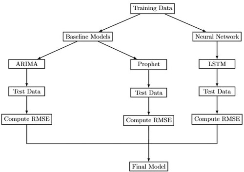
To model rainfall data, three potential models are considered. The flow chart in Figure 2 shows the skeleton of the steps involved in modelling the data set. Details of these steps are provided in the following sections.

Figure 2. Flow chart of data analysis steps.

2.5. Artificial neural network

An artificial neural network system is defined by Golden (1996) as an abstract mathematical model inspired by brain structures, mechanisms and functions.

The impulse is carried towards the biological neuron through dendrites and activated in the nucleus after weighting its effect. Then impulse carried away from the neuron through axon to axon terminals. Similarly in artificial neural network (ANN), input data are combined together then activate with certain activation function. Then the output of ANN has been given.

Biological neural networks work well after a number of training with trial and error. Likewise, artificial neural network learns after a number of iterations. After each iteration, the error made by the trial would back-propagate for updating the system.

Like biological neural network, an artificial architecture is designed to solve different problems. Among the ANN, the recurrent neural network is one. It is designed to handle data that have a sequential structure.

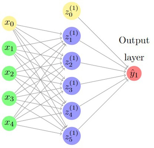
2.5.1. Single layer preceptron (SLP)

Single layer preceptron is a feed-forward algorithm involving only one hidden layer (see Figure 3). Each unit in the layer computes a weighted sum of its inputs of the form (3) $a_j=\sum _i{w}_{ji}{z}_i,$(3) where $z_i$ is the input and $w_{ji}$ denotes the weight associated with that connection. In this process, $a_j$ is activated using differentiable activation functions like tanh and $\text{sigmoid}\left(\sigma \right)$.

Figure 3. Single layer preceptron.

Usually, at initial step weights are given randomly. So, we need to determine suitable values for the weights in the network. This involves the minimization of an appropriate error function, such as root mean square error, mean absolute error and other measures of error in the estimation. Then, we update the weight matrix we have. By this one can see that, information feeds into the network and follows forward propagation, and information obtained from error function, which is gradient, back propagates to update the weight.

Let us denote an error function due to n-th pattern by $E^n$. We look for a combination of weights $w_{ji}$ that minimizes the error function. Mathematically this can be found by solving (4) $\frac{\mathrm{\partial }{E}^n}{\mathrm{\partial }{w}_{ji}}=0.$(4) But, the weight is related to the error through the output $a_j$. We can therefore apply the chain rule for partial derivatives to give (5) $\frac{\mathrm{\partial }{E}^n}{\mathrm{\partial }{w}_{ji}}=\frac{\mathrm{\partial }{E}^n}{\mathrm{\partial }{a}_j}\frac{\mathrm{\partial }{a}_j}{\mathrm{\partial }{w}_{ji}}.$(5) Then, the derivative of the total error E can be obtained by summing the derivation over all patterns: (6) $\frac{\mathrm{\partial }E}{\mathrm{\partial }{w}_{ji}}=\sum _n\frac{\mathrm{\partial }{E}^n}{\mathrm{\partial }{w}_{ji}}.$(6) On this basis, we update the weight and this approach is called (standard) back propagation.

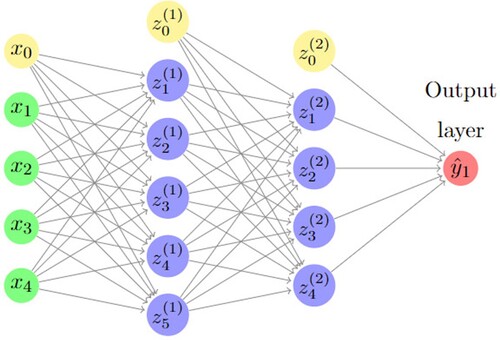
2.5.2. Multilayer preceptron (MLP)

Multilayer preceptron is a version of SLP. It involves a number of hidden layers. The feed forward and back propagation involve similar approach with SLP. To demonstrate how the network connects together, an MLP with two hidden layers is given in Figure 4.

Figure 4. A multilayer preceptron with two hidden layers.

We minimize the loss function by looking for optimal values for weights. This could achieve by taking first-order derivative of the function with respect to weight. For weights not connected to the output, the equations are derived by the chain rule in the same way as the standard backpropagation.

2.6. Recurrent neural network

The recurrent neural network (RNN) is a non-parametric algorithm in which we try to model the functional form of the data by learning from the data, through its architecture and parameters. The idea behind this approach is to make use of sequential information.

In its small shell, the RNN is usually called Vanilla RNN. With this approach, we usually face a problem of vanishing or exploding gradients. One way of getting around this is to use long short-term memory (Hochreiter, 1998), which is a variant of the RNN.

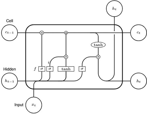
2.6.1. Long short-term memory

The Long Short-Term Memory (LSTM) block consists of input, output and forget gates (Hochreiter & Schmidhuber, 1997). Each of these gates has its own functionality. In addition to these gates, the LSMT involves the number of states: cell state, candidate state.

The forget gate makes the LSTM model long-term dependency. This gate tells the process how much of information from the input $x_t$ and the last output $h_{t-1}$ to keep. Here, 0 is forgetting everything and 1 is holding on everything.

The input gate declares how much of the information should be stored in the cell state. It prevents the cell from storing unnecessary data.

Lastly, the output gate decides how much of the memory cell to expose the block output. To illustrate how information flows throw the architecture of LSTM model let us see Figure 5.

Figure 5. Illustration of an LSTM architecture.

The mathematical computations done at each stage are given as follows: (7) $\begin{array}{rl}\text{forget gate:}& {\mathbf{f}}_t=\sigma ({\mathbf{W}}_f{\mathbf{x}}_t+{\mathbf{R}}_f{\mathbf{h}}_{t-1}+{\mathbf{b}}_f)=\sigma \left({\overline{\mathbf{f}}}_t\right),\end{array}$(7) (8) $\begin{array}{rl}\text{input get:}& {\mathbf{i}}_t=\sigma ({\mathbf{W}}_i{\mathbf{x}}_i+{\mathbf{R}}_i{\mathbf{h}}_{t-1}+{\mathbf{b}}_i)=\sigma \left({\overline{\mathbf{i}}}_t\right),\end{array}$(8) (9) $\begin{array}{rl}\text{cadidate state:}& {\mathbf{z}}_t=\tanh ({\mathbf{W}}_c{\mathbf{x}}_c+{\mathbf{R}}_c{\mathbf{h}}_{t-1}+{\mathbf{b}}_c)=\tanh \left({\overline{\mathbf{z}}}_t\right),\end{array}$(9) (10) $\begin{array}{rl}\text{cell state:}& {\mathbf{c}}_t={\mathbf{f}}_t\odot {\mathbf{c}}_{t-1}+{\mathbf{i}}_t\odot {\mathbf{z}}_t,\end{array}$(10) (11) $\begin{array}{rl}\text{cell get:}& {\mathbf{o}}_t=\sigma ({\mathbf{W}}_o{\mathbf{x}}_o+{\mathbf{R}}_o{\mathbf{h}}_{t-1}+{\mathbf{b}}_o)=\sigma \left({\overline{\mathbf{o}}}_t\right),\end{array}$(11) (12) $\begin{array}{rl}\text{output:}& {\mathbf{h}}_t={\mathbf{o}}_t\odot \tanh \left({\mathbf{c}}_t\right),\end{array}$(12) where ${\mathbf{x}}_t$ is the input vector at time t, $\mathbf{W}$ and $\mathbf{R}$ are weight matrices, ${\mathbf{b}}_t$ is the vector of bias, σ and tanh are activation/transfer functions and ⊙ denotes element wise multiplications. Hochreiter and Schmidhuber (1997) provided the detail of the algorithm. On the basis of this algorithm we optimize and generalize the model. The algorithm for a single state's delta inside the LSTM block is calculated as Greff et al. (2017): (13) $\begin{array}{rl}\delta {\mathbf{h}}_t& ={\mathit{\theta }}_t+{\mathbf{R}}_f^{\mathrm{\top }}\delta {\mathbf{f}}_{t+1}+{\mathbf{R}}_i^{\mathrm{\top }}\delta {\mathbf{i}}_{t+1}+{\mathbf{R}}_c^{\mathrm{\top }}\delta {\mathbf{z}}_{t+1}+{\mathbf{R}}_o^{\mathrm{\top }}\delta {\mathbf{o}}_{t+1},\end{array}$(13) (14) $\begin{array}{rl}\delta \overline{{\mathbf{o}}_t}& =\delta {\mathbf{h}}_t\odot \tanh \left({\mathbf{c}}_{\mathbf{t}}\right)\odot {\sigma }^{\mathrm{\prime }}\left(\overline{{\mathbf{o}}_t}\right),\end{array}$(14) (15) $\begin{array}{rl}\delta {\mathbf{c}}_t& =\delta {\mathbf{h}}_t\odot {\mathbf{o}}_t\odot {\tanh }^{\mathrm{\prime }}\left({\mathbf{c}}_t\right)+\delta {\mathbf{c}}_{t+1}\odot {\mathbf{f}}_{t+1},\end{array}$(15) (16) $\begin{array}{rl}\delta {\mathbf{f}}_t& =\delta {\mathbf{c}}_t\odot {\mathbf{c}}_{t-1}\odot {\sigma }^{\mathrm{\prime }}\left({\overline{\mathbf{f}}}_t\right),\end{array}$(16) (17) $\begin{array}{rl}\delta {\mathbf{c}}_t& =\delta {\mathbf{c}}_t\odot {\mathbf{z}}_t\odot {\sigma }^{\mathrm{\prime }}\left({\overline{\mathbf{i}}}_t\right),\end{array}$(17) (18) $\begin{array}{rl}\delta {\mathbf{z}}_t& =\delta {\mathbf{c}}_t\odot {\mathbf{i}}_t\odot {\tanh }^{\mathrm{\prime }}\left({\overline{\mathbf{z}}}_t\right).\end{array}$(18) Here ${\mathit{\theta }}_t$ is the vector of deltas that propagates back into the system to update the parameters.

Finally, the gradients for the weights are calculated as follows: (19) $\begin{array}{rl}\delta {\mathbf{W}}_{\star }& =\sum _{t=0}^T〈\delta {\star }_t,{\mathbf{x}}_t〉,\end{array}$(19) (20) $\begin{array}{rl}\delta {\mathbf{R}}_{\star }& =\sum _{t=0}^{T-1}〈\delta {\star }_t,{\mathbf{h}}_t〉,\end{array}$(20) (21) $\begin{array}{rl}\delta {\mathbf{b}}_{\star }& =\sum _{t=0}^T\delta {\star }_t,\end{array}$(21) where ⋆ can be any of $\{\overline{\mathbf{z}},\overline{\mathbf{i}},\overline{\mathbf{f}},\overline{\mathbf{o}}\}$, and $〈{\ast }_1,{\ast }_2〉$ denotes the outer product of two vectors.

2.6.2. Model evaluation and improvement

As a part of finding optimal architecture, we need to add or minimize the number of layers and nodes of each layer. In our case, there is no need to have a larger number of layers (three or a maximum of four is supposed to be sufficient) as the pattern of rainfall data seems a sinusoidal wave.

With a pre-defined number of layers, nodes and other parameters, we have tried to fit the model into the data. Then the performance of the model is measured by root mean squared error (RMSE). The construction of the architecture is done iteratively until the one with the lowest RMSE is found.

2.7. Comparing performance of the models

Once the parameter of the LSTM model is optimized in such a way that the model has good generalization for the test data, we compare it with two competing models.

The first model is the ARIMA model which is constructed using the Box and Jenkins (1976) approach. The other is in Prophet Taylor and Letham (2018a, 2018b) which is an open-source software released by Facebook's Core Data Science team. It provides an automatic forecasting.

Having these two potential competitive models, we test the reduction/increment in RMSE against LSTM.

2.7.1. Prophet model

The time series model is decomposed into three main model components: trend ($g\left(t\right)$), seasonality ($s\left(t\right)$) and holidays ($h\left(t\right)$). The specification of the model is similar to the generalized linear model, a class of regression models with potentially non-linear smoothers applied to the regressors (which is only time in the Prophet model). This additive model is given as follows: (22) $y\left(t\right)=g\left(t\right)+s\left(t\right)+h\left(t\right)+{ϵ}_t.$(22) The components of each model have their functional representation.

Trend model. In modelling Prophet, we relied on linear trend with change points (i.e., unsaturated growth). Here the model is: (23) $g\left(t\right)=(k+\mathbf{a}(t{)}^{\mathrm{\top }}\mathit{\delta })t+(m+\mathbf{a}\left(t{)}^{\mathrm{\top }}\mathit{\gamma }\right),$(23) where k is the growth rate, δ is the change in rate that occurs at time $s_j,j=1,2,\dots ,S$ (S denotes number of change points), m is the offset parameter, ${\gamma }_j$ is set to $-s_j{\delta }_j$ to make the function continuous and (24) $a_j\left(t\right)=\{\begin{array}{ll}1,& \mathrm{i}\mathrm{f}t\ge s_j,\\ 0,& \mathrm{o}\mathrm{t}\mathrm{h}\mathrm{e}\mathrm{r}\mathrm{w}\mathrm{i}\mathrm{s}\mathrm{e}.\end{array}$(24) The prior distributions of $k,m,\delta$, and other quantities are specified to fit the model.

Seasonality. To model seasonal components, they relied on a standard Fourier series. The seasonal effects are approximated by (25) $s\left(t\right)=\sum _{n=1}^N(a_n\cos \left(\frac{2\text{π}nt}{P}\right)+b_n\cos \left(\frac{2\text{π}nt}{P}\right))=\mathbf{X}\left(t\right)\text{β},$(25) where $\mathbf{X}\left(t\right)=[\cos (\frac{2\text{π}\left(1\right)t}{P}),\sin (\frac{2\text{π}\left(1\right)t}{P}),\dots ,\cos (\frac{2\text{π}Nt}{P}),\cos (\frac{2\text{π}Nt}{P}\left)\right]$, $\text{β}=[a_1,b_1,a_N,b_N{]}^{\mathrm{\top }}$, P denotes the regular period we expect the time series to have and N is the order at which the series is truncated to apply a low-pass filter to seasonality. The choice of N is automated using a model selection procedure such as AIC. The parameter $\text{β}\sim N$ $(0,{\sigma }^2)$, which imposes smoothing on the seasonality.

Holidays and events. These effects are common in economic data and data which is affected by holidays and events. The detail of theory and computation about holidays and events effect is given in Taylor and Letham (2018a). Since variability in rainfall data could not be due to holidays and events effect, we did not take into account this component.

Model fitting. For model fitting, Stan's L-BFGS (Carpenter et al., 2017), which is a quasi-Newton algorithm provided to find modes of the density, was used to find a maximum a posterior estimate.

In Stan's L-BFGS optimization, the priors are found as follows: (26) $\begin{array}{rl}k& \sim N(0,5),\end{array}$(26) (27) $\begin{array}{rl}m& \sim N(0,5),\end{array}$(27) (28) $\begin{array}{rl}ϵ& \sim N(0,0.5),\end{array}$(28) (29) $\begin{array}{rl}\delta & \sim \mathrm{L}\mathrm{a}\mathrm{p}\mathrm{l}\mathrm{a}\mathrm{c}\mathrm{e}(0,\tau ),\end{array}$(29) (30) $\begin{array}{rl}\text{β}& \sim N(0,{\sigma }^2).\end{array}$(30) Then the linear likelihood for $y\left(t\right)$ is given by $y\left(t\right)\sim N\left(\right(k+\mathbf{A}\mathit{\delta }\left)t\right)+\left(\right(m+\mathbf{A}\mathit{\gamma })+(\mathbf{X}\text{β}),{\sigma }^2),$ where $\mathbf{X}$ denotes a matrix of seasonality feature for each observation and the changing point in $a\left(t\right)$ is given in matrix $\mathbf{A}$. The parameters τ and σ are controls for amount of regularization on the model change points and seasonality respectively. These regularizers avoid overfitting.

3. Result and discussion

3.1. Clustering and centering

To prepare the dataset for clustering, we used similar sliding window ($=20$), alphabet size ($=3$) and length of PAA ($=5$) to construct a matrix of bag of word (BOW) representation. Among possible word representations for the pattern of the dataset, we extracted those having a non-zero count at least for one dataset. The total number of extracted word representations is 161. Table 1 shows how the dataset is formed using the BOW representation.

Table 1. Matrix of BOW representation for the rainfall data.

SAX	Abay Sheleko	Addis Ababa	…	Melkasa
ccabb	0	0	…	1
aaacb	1	0	…	0
aacab	2	2	…	0
aacba	2	0	…	0
aacbb	2	0	…	2
⋮	⋮	⋮	⋮	⋮

Once the dataset was represented using BOW representation, the k-means algorithm was used for clustering purpose. From the data, we found that the optimal number of clusters was 7. This number was found to be optimal after a number of iteration for the different number of clusters. The ratio of between sum of squares to total sum of squares was about 80%. This indicates that, about 80% measure of the total variance in the data set is explained by the clustering.

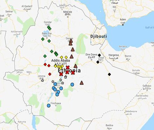
By this we have created seven rainfall regions. The spatial distribution of these homogenized rainfall stations is given in Figure 6. Stations with the same shape and colour belong to the same region. (i.e., Cluster 1 = Cross and Red; Cluster 2 = Diamond and Yellow; Cluster 3 = Plus and Green; Cluster 4 = Circle and Blue; Cluster 5 = Triangle and Brown; Cluster 6 = Star and Grey; Cluster 7 = Diamond and Black).

Figure 6. Spatial distribution of homogenized rainfall stations.

Next, we centre the datasets of the same cluster, using spatial averaging methods.

3.2. Descriptive statistics

A total of 48 meteorological stations having rainfall data with not more than 10% missing values were selected.

Once the missing values (10% or less) and outliers are fixed for each of the stations, spatial averages have been computed following the steps in Section 3.1. The time series plot of rainfall region 1 is given below (Figure 7). The rest of these plots for other rainfall regions are given in Appendix.

Figure 7. Time series plot of region 1.

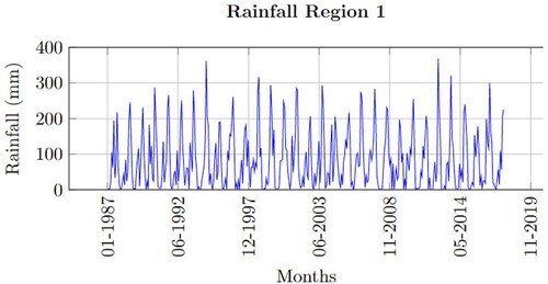
The time series plots revealed that the seasonality behaviour in the spatially averaged datasets is being masked by some form of irregularity. This is common in averaging sinusoidal wave with different wavelengths and amplitudes.

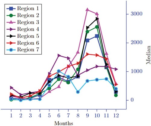
The Skewness of the datasets is computed to choose an appropriate measure of central tendency. From Table 2, one can see that most of the rainfall regions have skewness greater than 0.5, which shows that the datasets deviate from symmetry. Due to this, we choose median as a measure of central tendency.

Table 2. Skewness and coefficient of variation.

	Rainfall regions
Statistics	Reg1	Reg2	Reg3	Reg4	Reg5	Reg6	Reg7
Skewness	1.01	1.13	0.97	0.37	1.22	0.19	1.05
Coef. Var.	0.99	1.07	1.06	0.62	0.95	0.71	0.91

From Table 2, furthermore, we noticed that Region 2 and Region 3 show higher inconsistency relative to the other regions, as the values of coefficient of variation are greater than 1.

The median values are plotted in Figure 8, which shows how the median values of rainfall regions behave over the 12 months.

Figure 8. Monthly median of rainfall regions.

3.3. Baseline models

We began by fitting the ARIMA and Prophet models before fitting the LSTM model to the dataset. Then, we compare the RMSE of ARIMA with the RMSE of the well-tuned hyperparameter LSTM model. Moreover, we compare the RMSE of the Prophet models with that of the LSTM model.

To fit ARIMA to the dataset, we used the automatic ARIMA (auto.arima) function in the fpp2 package for R-Software (Hyndman et al., 2018; Hyndman & Khandakar, 2008). While fitting this model the dataset is split into training (= 90%) and test (= 10%). The result of this model is given in Table 3.

Table 3. ARIMA and prophet models for the rainfall data.

Clusters	Model	RMSE of train	RMSE of test
Region 1	ARMA(2, 1)	62.4699	72.4940
	Prophet	38.7272	283.755
Region 2	ARMA(2, 2)	54.6949	71.0454
	Prophet	29.7501	212.915
Region 3	ARMA(2, 1)	61.1237	82.8129
	Prophet	34.2161	312.491
Region 4	ARMA(2, 2)	51.3413	54.8593
	Prophet	39.7526	78.8866
Region 5	ARMA(2, 1)	69.0534	93.9794
	Prophet	40.7781	279.093
Region 6	AR(1)	51.2755	65.5314
	Prophet	33.2418	89.2924
Region 7	MA(1)	42.0095	56.2437
	Prophet	29.7944	60.3597

The models are shown to satisfy stationarity and invertibility conditions. We have checked whether given long memory models are invertible and stationary using IdentInvertQ function developed in R (Veenstra, 2012). The result we found (see Table 4) shows that all of the models are stationary and invertible.

Table 4. ARMA models' test of stationarity and invertibility.

	Autoregressive		Moving average
Clusters	ar1	ar2	ma1	ma2	IdentInvertQ
Region 1	1.3628	−0.6393	−0.8904	–	True
Region 2	1.3988	−0.6912	−0.6901	−0.2010	True
Region 3	1.5635	−0.8391	−0.8241	–	True
Region 4	1.4160	−0.6342	−1.0674	0.2141	True
Region 5	1.3646	−0.6467	−0.8663	–	True
Region 6	0.5713	–	–	–	True
Region 7	–	–	0.3259	–	True

In addition to the ARMA model, results of RMSE of potential seasonal model, which is called Prophet, are given in Table 3. In this table, their corresponding RMSEs are given for each rainfall region.

3.4. Long short-term memory model

3.4.1. Model identification

After analysing the results of the baseline models, we fitted the LSTM model to the dataset anticipating a reduction of root mean squared error (RMSE) both for training and test data sets. In addition, we depend on stability in the reduction of loss for both training and validation data sets while fitting the LSTM.

To have a well-fitted model to the data set, we considered a combination of Input Size (1 to 35), the dimension of hidden layers(0 to 3), size of neurons (1 to 35), Epoch (1 to 1000) and batch size (1 to 50). Also, we set value regularization parameters ${\text{β}}_1$ and ${\text{β}}_2$ within the range of 0.001 –0.3. We found optimal input size for all datasets to be 20 within the range of 1–35 after feeding the data with these setting into the network.

In Table 5, a well-fitted architecture for all rainfall regions is given. The resulting RMSE for both train and test dataset is also given in the table. The total number of parameters trained and estimated was 3280, 2331, 3009, 1301, 5006, 4736 and 2246 for rainfall region 1 to region 7 respectively.

Table 5. LSTM model.

	Neuron size			Batch	Regularizers		RMSE	RMSE
Clusters	Layer 1	Layer 2	Epoch	size	${\text{β}}_1$	${\text{β}}_2$	Train	Test
Region 1	20	14	480	11	0.001	0.22	29.44	41.27
Region 2	15	10	250	23	0.001	0.22	29.68	37.33
Region 3	18	10	189	10	0.010	0.60	33.18	37.22
Region 4	10	5	217	35	0.001	0.12	35.40	40.66
Region 5	25	15	300	40	0.001	0.50	36.49	61.14
Region 6	25	5	300	35	0.001	0.13	28.40	46.40
Region 7	15	5	520	15	0.001	0.20	21.36	36.46

3.4.2. Diagnostic plot for goodness of fit

A tool we used for goodness of fit for the model is the plot of loss against epoch. In Figure 9, plot of loss against epoch for the LSTM model of rainfall region 1 is given.

Figure 9. A plot of loss for the LSTM model of region 1.

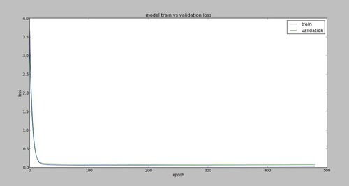
Monotonicity in the reduction of loss after each epoch shows that the architecture has learned more about the nature of the data's pattern. Since there are no ups and downs in the graph of the losses, the system does not underfit nor overfit. Furthermore, the monotonicity in the structure of the losses justifies the goodness of fit of the model to the dataset.

3.4.3. Model comparison against baseline models

In Tables 4 and 5, the results of both baseline models and the proposed model were presented. The Prophet is more likely to have lower RSME which is closer to LSTMs' than the ARMA model for training dataset. On the other hand, ARIMA works better than the Prophet when it comes to the out-sample (test) data.

When we have a look at the reduction of RSME for these potential models, as a general rule, LSTM shows the lowest RMSE for both training and test dataset. These show that LSTM gives us a better reduction in bias and variance when compared with either of the baseline models. This suggests that the LSTM architectures have tuned well for generalization/forecasting over baseline models. Furthermore, the diagnostic plots support the goodness of fit of the model.

4. Discussion

Homogenization of rainfall stations of Ethiopia was the issue we have addressed in our study. The same problem has been solved by Tsidu (2012) based on creating grid regions. Tsidu (2012) has created nine rainfall regions. In our case, we relied on extracting the local and global pattern of the dataset using a Back-of-Word algorithm and implementing k-means. Finally, we found seven homogenized rainfall regions.

The method we used to create homogenized rainfall regions was completely different from the one which was done by Tsidu (2012). Because our ultimate goal was to model the data set, we also excluded rainfall stations with high missing values. On the areas of the dataset, we were able to cluster. We saw that our results coincide with the results in Tsidu (2012).

In our case, the rainfall regions are centred by spatial averaging approach. The pattern of the rainfall regions was represented by the data generated using a spatial average.

In this paper, we used a technique known as ‘Long Short Memory Term’ to which we feed dataset to construct an artificial neural network model for each homogenized rainfall region. The hyperparameters of the LSTM have been tuned so that the architecture captures the dynamics of datasets.

Well-tuned LSTM models show the strongest performance compared to ARIMA and Facebook's Prophet. These results are in line with the work of Jiang and Zhang (2018), in which they compared LSTM with different settings, some involving wavelet or Kalman filter and other with no filter. Each variant of LSTM resulted in better performance than the Prophet and ARIMA models.

On the other hand, our finding is in contrast to the work of Dabakoglu (2019), who revealed that ARIMA model is the best model when compared with LSTM and Prophet while modelling a monthly beer production. This is due to the fact that while modelling LSTM, Dabakoglu only takes a single lag value. In our situation, we've chosen a set of 20 lagged values (i.e., an optimal lag selected after iterations).

In this study, LSTM is found to be prone to the problem relating to the gradient of errors backpropagate into the network while estimating the parameters of the network. These problems are usually known as vanishing and exploding gradients, which is common in the vanilla RNN architecture.

In our work, the diagnostic plot shows high power of LSTM to overcome overfitting and underfitting. This is in line with the original work of Hochreiter (1998).

The monotonicity reduction in the value of losses of training over epochs shows that the architecture is able to capture high variance in the pattern of training datasets. This indicates that the model is not underfitted. So there is no problem of vanishing gradients.

Besides these, a similar reduction of losses for test data set indicates that the model performs well for the out-sample data set. In addition, overfitting problem is not observed in LSTM models. Therefore, over the iterations of the network there is no problem of gradient exploding.

Thus loss of strong seasonal behaviour due to spatial averages did not affect the performance of LSTM to capture the pattern of dataset as it is usually the contrary in the case of both ARIMA and Prophet models. This suggests that LSTM can be considered as the best model for modelling rainfall data when compared to the baseline models.

5. Conclusion

In this study, we took 147 rainfall stations and created homogenized rainfall stations. Starting with selecting stations having missing values less than 10%, we fixed missing values by spatial interpolation, and outliers were fixed automatically using the ‘tsoutliers’ package developed in R. Then both local and global patterns of the dataset have been extracted using Back-of-Word algorithm. K-means clustering was implemented on the matrix generated by a Back-of-Word algorithm. After a number of iterations, the number of optimal clusters was found to be 7.

Each of these clusters is considered as homogeneous rainfall regions. The rainfall data in each region are centred by spatial averaging approach, in which we took into account resolution parameters to weight the dataset. By these, we found seven univariate time series datasets. Each of them centres the region they are generated from.

In this study, our interest was not only to create homogenized rainfall regions and centre them but also constructing appropriate predictive models which could capture the pattern of these datasets.

To capture the pattern of the datasets, we have constructed three potential models. Two of them, ARIMA and Facebook's Prophet, are considered as baseline models and the LSTM model, proposed in this study.

RMSE was the tool we used to compare the performance of the baseline models against LSTM model both on training and testing datasets. Well-tuned LSTM models showed the lowest RMSE for both training and testing datasets for all rainfall regions.

Besides, the diagnostic plot has been constructed for all LSTM models to see how the loss generated over a number of epochs behaves. And we found monotonicity reduction, i.e., non-increment nature structure.

Based on the lowest value of RMSE of LSTM in comparison to the baseline models' and the diagnostic plot, we could say the proposed LSTM models are well tuned to capture the pattern of the dataset. Therefore, the model was found to be a potential predictive model.

Acknowledgements

We thank Dr Yaping Wang for his helpful comments on an earlier version of this manuscript.

Disclosure statement

No potential conflict of interest was reported by the author(s).

Additional information

Funding

The work was supported by National Natural Science Foundation of China (Grant numbers: 11771146, 11831008, 81530086).

Appendix

References

- Abbot, J., & Marohasy, J. (2018). Forecasting of medium-term rainfall using Artificial Neural Networks: Case studies from Eastern Australia. In T. V. Hromadka & P. Rao (Eds.), Engineering and Mathematical Topics in Rainfall (pp. 33–56). Books on Demand. https://doi.org/10.5772/intechopen.72619.
- Berhanu, B., Seleshi, Y., & Melesse, A. M. (2014). Surface water and groundwater resources of ethiopia: Potentials and challenges of water resources development. In A. Melesse, W. Abtew, & S. Setegn (Eds.), Nile River Basin (pp. 97–117). Springer. https://doi.org/10.1007/978-3-319-02720-3_6
- Box, G. E. P., & Jenkins, G. M (1976). Time series analysis. Forecasting and control. In G. C. Reinsel (Ed.), Holden-day series in time series analysis (Revised ed.) Holden-Day.
- Brownlee, J. (2016). Time series prediction with lstm recurrent neural networks in Python with Keras. Available at: machinelearningmastery.com.
- Carpenter, B., Gelman, A., Hoffman, M. D., Lee, D., Goodrich, B., Betancourt, M., Brubaker, M., Guo, J., Li, P., & Riddell, A. (2017). Stan: A probabilistic programming language. Journal of Statistical Software, 76(1), 1–32. https://doi.org/10.18637/jss.v076.i01
- Chen, C., & Liu, L.-M. (1993). Joint estimation of model parameters and outlier effects in time series. Journal of the American Statistical Association, 88(421), 284–297. https://doi.org/10.2307/2290724
- Dabakoglu, C. (Jun 2019). Time series forecasting—Arima, LSTM, Prophet with python. Online. Retrieved June 30, 2019.
- Golden, R. M. (1996). Mathematical methods for neural network analysis and design. MIT Press.
- Greff, K., Srivastava, R. K., Koutník, J., Steunebrink, B. R., & Schmidhuber, J. (2017). Lstm: A search space Odyssey. IEEE Transactions on Neural Networks and Learning Systems, 28(10), 2222–2232. https://doi.org/10.1109/TNNLS.2016.2582924
- Haining, R. P., & Haining, R. (2003). Spatial data analysis: Theory and practice. Cambridge University Press.
- Hijmans, R. J. (2017). Geosphere: Spherical trigonometry. R package version 1.5-7.
- Hochreiter, S. (1998). Recurrent neural net learning and vanishing gradient. International Journal of Uncertainity, Fuzziness and Knowledge-Based Systems, 6(2), 107–116. https://doi.org/10.1142/S0218488598000094
- Hochreiter, S., & Schmidhuber, J. (1997). Long short-term memory. Neural Computation, 9(8), 1735–1780. https://doi.org/10.1162/neco.1997.9.8.1735
- Hyndman, R. J. (2013). FPP data for “forecasting: Principles and practice”. R package version 0.5.
- Hyndman, R., Athanasopoulos, G., Bergmeir, C., Caceres, G., Chhay, L., O'Hara-Wild, M., Petropoulos, F., Razbash, S., Wang, E., & Yasmeen, F. (2018). forecast: Forecasting functions for time series and linear models. R package version 8.4.
- Hyndman, R. J., & Khandakar, Y. (2008). Automatic time series forecasting: The forecast package for R. Journal of Statistical Software, 27(3), 1–22. https://doi.org/10.18637/jss.v027.i03
- Jiang, Y., & Zhang, Y. (2018). Exploration of predicting power of Arima, Facebook Prophet and lstm on time series. Stanford University. Online. Retrieved June 30, 2019.
- Lin, J., Keogh, E., Lonardi, S., & Patel, P. (2002). Finding motifs in time series. In Proc. of the 2nd workshop on temporal data mining (pp. 53–68).
- Lin, J., Keogh, E., Wei, L., & Lonardi, S. (2007). Experiencing sax: A novel symbolic representation of time series. Data Mining and Knowledge Discovery, 15(2), 107–144. https://doi.org/10.1007/s10618-007-0064-z
- Lin, J., & Li, Y. (2009). Finding structural similarity in time series data using bag-of-patterns representation. In M. Winslett (Ed.), International conference on scientific and statistical database management (pp. 461–477). Springer. https://doi.org/10.1007/978-3-642-02279-1_33
- Longley, P. A., Goodchild, M. F., Maguire, D. J., & Rhind, D. W. (2005). Geographic information systems and science (2nd ed.). John Wiley & Sons.
- Shen, S. S. P. (2017). R programming for climate data analysis and visualization: Computing and plotting for NOAA data applications. John Wiley & Sons.
- Strauß, M. (2018). Time series forecasting with LSTMS and Prophet, nov. Online. Retrieved June 30, 2019.
- Taylor, S. J., & Letham, B. (2018a). Forecasting at scale. The American Statistician, 72(1), 37–45. https://doi.org/10.1080/00031305.2017.1380080
- Taylor, S. J., & Letham, B. (2018b). Prophet: Automatic forecasting procedure. R package version 0.4.
- Tsidu, G. M. (2012). High-resolution monthly rainfall database for ethiopia: Homogenization, reconstruction, and gridding. Journal of Climate, 25(24), 8422–8443. https://doi.org/10.1175/JCLI-D-12-00027.1
- Veenstra, J. Q. (2012). Persistence and anti-persistence: Theory and software [PhD thesis]. Western University.