Locally R-optimal designs for a class of nonlinear multiple regression models

Abstract

This paper concerns with optimal designs for a wide class of nonlinear models with information driven by the linear predictor. The aim of this study is to generate an R-optimal design which minimizes the product of the main diagonal entries of the inverse of the Fisher information matrix at certain values of the parameters. An equivalence theorem for the locally R-optimal designs is provided in terms of the intensity function. Analytic solutions for the locally saturated R-optimal designs are derived for the models having linear predictors with and without intercept, respectively. The particle swarm optimization method has been employed to generate locally non-saturated R-optimal designs. Numerical examples are presented for illustration of the locally R-optimal designs for Poisson regression models and proportional hazards regression models.

Keywords:

• Poisson regression models
• proportional hazards models
• R-optimality
• particle swarm optimization

1. Introduction

Generalized linear models (GLMs) have been used quite effectively in statistical modelling but the associated design issues are undoubtedly challenging, since the intensity function within their information matrices depends on the value of the linear predictor, which means that the optimal designs are related to the unknown parameters. Following Konstantinou et al. (2014), we note that the information matrix of the proportional hazards regression models used in survival analysis also has the same feature when type I and random censoring are considered, and their intensity functions, which are similar to Poisson regression models and negative binomial regression models, are strictly monotonic rather than a symmetric structure that appears in the logistic and probit models. In this paper, we focus on such models with monotonic intensity functions.

In this direction, there is increasing interest in determining optimal designs under various criteria, especially for models with multiple covariates. Initial work was done by Konstantinou et al. (2014) who provided analytical results of D- and c-optimal designs for this class of models with only one covariate. Subsequently, Schmidt and Schwabe (2015) extended the results concerning D-optimality to one-dimensional discrete design space. For multiple regression, Schmidt and Schwabe (2017) determined D-optimal designs by identifying a complete subclass, which contains the results of Russell et al. (2009) for the Poisson regression model as a special case. Radloff and Schwabe (2019) gave a construction method of D-optimal designs when the design region is a k-dimensional ball. Recently, Schmidt (2019) systematically characterized c-, L- and ${\mathrm{\Phi }}_k$-optimal designs for models with a single covariate and for multiple regression with an arbitrary number of covariates.

It should be noted that the linear predictor in the previously mentioned literature always includes an intercept term. The intercept in GLMs and proportional hazards regression models with censoring, respectively, characterizes the expected mean and expected survival time when all the explanatory variables are equal to zero. In this case, the linear predictor reflects the influence of all the unobserved fixed variables in these models. As pointed out by Idais and Schwabe (2021), when the intercept is significantly zero, i.e., the average impact of all the unobserved fixed variables is significantly zero, one may claim that the model includes probably most variables which explain the outcome. For the gamma models without intercept, Idais and Schwabe (2021) obtained some explicit solutions of D- and A-optimal designs in some multi-linear cases, including the two-factor model with interaction.

This paper aims to provide a characterization of R-optimality for multiple regression models with and without intercept. It is well known that the R-optimality criterion proposed by Dette (1997) has a nice statistical interpretation, namely minimizing the volume of the Bonferroni rectangular confidence region of the regression parameters. Moreover, it satisfies an extremely useful invariance property which allows an easy calculation of optimal designs on many linearly transformed design spaces. This optimality has been frequently applied to the cases of multi-response experiments, multi-factor experiments and mixture experiments, see, e.g., X. Liu and Yue (2020), P. Liu et al. (2022) and Hao et al. (2021) for some recent references.

In general, the dependence of designs on parameters whose values are unknown a priori occurs in nonlinear regression models. Hence, utilizing a pre-specified parameter value we can obtain the so-called locally optimal designs in accordance with Chernoff (1953). In this paper, we concentrate on the construction of locally optimal designs and take R-optimal designs to replace locally R-optimal designs for simplicity. Some general notations and a brief introduction of the R-criterion are presented in Section 2. In Sections 3 and 4, we analytically and numerically determine R-optimal designs for models having an intensity function which only depends on the value of the linear predictor with and without intercept, respectively. A brief discussion is given in Section 5. All proofs are included in the Appendix.

2. Model specification and R-optimality criterion

Throughout the paper, we focus on a class of nonlinear multiple regression models with information driven by the linear predictor defined on a given design region $\mathcal{X}$, and consider the approximate designs ξ of the form $\xi =\left\{\begin{array}{cccc}{\mathit{x}}_1& {\mathit{x}}_2& \cdots & {\mathit{x}}_m\\ {\omega }_1& {\omega }_2& \cdots & {\omega }_m\end{array}\right\},{\mathit{x}}_i\in \mathcal{X},0⩽{\omega }_i⩽1,\sum _{i=1}^m{\omega }_i=1$or simply $\xi =\{{\mathit{x}}_i;{\omega }_i{\}}_{i=1}^m$ (see Silvey, 1980, p. 15). The Fisher information matrix of ξ with independent observations is assumed to be (1) $\mathit{M}(\xi ,\text{β})={\int }_{\mathcal{X}}Q\left(\mathit{f}\right(\mathit{x}{)}^{\mathrm{\top }}\text{β}\left)\mathit{f}\right(\mathit{x}\left)\mathit{f}\right(\mathit{x}{)}^{\mathrm{\top }}\mathrm{d}\xi \left(\mathit{x}\right)=\sum _{i=1}^m{\omega }_{i}Q\left(\mathit{f}\right({\mathit{x}}_i{)}^{\mathrm{\top }}\text{β}\left)\mathit{f}\right({\mathit{x}}_i\left)\mathit{f}\right({\mathit{x}}_i{)}^{\mathrm{\top }},$(1) where $Q\not\equiv 0$ is the intensity/efficiency function (see Fedorov, 1972, p. 39) which only depends on the value of the linear predictor, $\mathit{f}$ is a $p\times 1$ vector of known regression functions, and $\text{β}\in {\mathbb{R}}^p$ denotes the vector of p unknown parameters.

This kind of information matrix is common in the widely used generalized linear models, while it may also arise in other models such as the exponential regression models in proportional hazards parametrization with various censoring, including type I and random censoring (see Konstantinou et al., 2014) as well as other censoring distributions (see Schmidt & Schwabe, 2017). Following Konstantinou et al. (2014), we further assume that the intensity function Q satisfies the following conditions.

(A1)	$Q\left(\theta \right)$ is positive for all $\theta \in \mathbb{R}$ and twice continuously differentiable.
(A2)	The derivative $Q^{\mathrm{\prime }}\left(\theta \right)$ is positive for all $\theta \in \mathbb{R}$.
(A3)	The second derivative $g^{\mathrm{\prime }\mathrm{\prime }}\left(\theta \right)$ of the function $g\left(\theta \right)=1/Q\left(\theta \right)$ is injective.
(A4)	The function $Q\left(\theta \right)/Q^{\mathrm{\prime }}\left(\theta \right)$ is an increasing function.

It is clear that the intensity functions induced by Poisson regression models, negative binomial regression models and proportional hazards regression models with type I and random censoring abide by all the conditions above.

In what follows, we concentrate on the R-optimality of designs which minimizes the product of the diagonal entries of the inverse of the Fisher information matrix. A design ${\xi }^{\ast }\in \mathrm{\Xi }$ is called R-optimal if it minimizes (2) $\psi (\xi ,\text{β})=\prod _{j=1}^p{\left(\mathit{M}\right(\xi ,\text{β}{)}^{-1})}_{jj}=\prod _{j=1}^p{\mathit{e}}_{j,p}^{\mathrm{\top }}\mathit{M}(\xi ,\text{β}{)}^{-1}{\mathit{e}}_{j,p}$(2) over Ξ, where Ξ is the set of all designs with a non-singular information matrix on $\mathcal{X}$, and ${\mathit{e}}_{j,p}$ denotes the jth unit vector in ${\mathbb{R}}^p$. An important tool in optimal design theory is equivalence theorems that not only provide a characterization of the optimal design but also are the basis of many algorithms for their numerical construction (see, e.g., Yang et al., 2013; Freise et al., 2021). The following result gives the equivalence theorem for R-optimality.

Theorem 2.1

A design ${\xi }^{\ast }\in \mathrm{\Xi }$ is R-optimal if and only if (3) $\varphi (\mathit{x},\text{β})=Q\left(\mathit{f}\right(\mathit{x}{)}^{\mathrm{\top }}\text{β}\left)\mathit{f}\right(\mathit{x}{)}^{\mathrm{\top }}\mathit{M}({\xi }^{\ast },\text{β}{)}^{-1}\left(\sum _{j=1}^p\frac{{\mathit{e}}_{j,p}{\mathit{e}}_{j,p}^{\mathrm{\top }}}{{\mathit{e}}_{j,p}^{\mathrm{\top }}\mathit{M}({\xi }^{\ast },\text{β}{)}^{-1}{\mathit{e}}_{j,p}}\right)\mathit{M}({\xi }^{\ast },\text{β}{)}^{-1}\mathit{f}\left(\mathit{x}\right)⩽p$(3) holds for all $\mathit{x}\in \mathcal{X}$. Moreover, it is equal at the support points of the design ${\xi }^{\ast }$.

In Sections 3 and 4 the minimally supported designs (i.e., the so-called saturated designs) will appear as candidates for determining R-optimal designs. A design $\xi =\{{\mathit{x}}_i;{\omega }_i{\}}_{i=1}^m$ has minimal support if the number of support points is equal to the number of parameters, i.e., m = p. Let ${\mathit{D}}_{\omega }$ =$\mathrm{d}\mathrm{i}\mathrm{a}\mathrm{g}({\omega }_1,\dots ,{\omega }_m)$, $\tilde{\mathit{X}}$=${\mathit{Q}}^{1/2}\mathit{X}$ with $\mathit{X}=\left(\mathit{f}\right({\mathit{x}}_1),\dots ,\mathit{f}({\mathit{x}}_m){)}^{\mathrm{\top }}$ and ${\mathit{Q}}^{1/2}$=$\mathrm{d}\mathrm{i}\mathrm{a}\mathrm{g}(\sqrt{Q\left(\mathit{f}\right({\mathit{x}}_1{)}^{\mathrm{\top }}\text{β})},$ $\cdots ,\sqrt{Q\left(\mathit{f}\right({\mathit{x}}_m{)}^{\mathrm{\top }}\text{β})})$. Accordingly, the information matrix (1(1) $\mathit{M}(\xi ,\text{β})={\int }_{\mathcal{X}}Q\left(\mathit{f}\right(\mathit{x}{)}^{\mathrm{\top }}\text{β}\left)\mathit{f}\right(\mathit{x}\left)\mathit{f}\right(\mathit{x}{)}^{\mathrm{\top }}\mathrm{d}\xi \left(\mathit{x}\right)=\sum _{i=1}^m{\omega }_{i}Q\left(\mathit{f}\right({\mathit{x}}_i{)}^{\mathrm{\top }}\text{β}\left)\mathit{f}\right({\mathit{x}}_i\left)\mathit{f}\right({\mathit{x}}_i{)}^{\mathrm{\top }},$(1) ) for the design ξ can be decomposed as $\mathit{M}(\xi ,\text{β})$=${\tilde{\mathit{X}}}^{\mathrm{\top }}{\mathit{D}}_{\omega }\tilde{\mathit{X}}$. Furthermore, if the design ξ is saturated and the regression vectors located at the rows of $\mathit{X}$ are linearly independent, the following result exhibits the optimal weights of a design with minimal support for the R-optimality criterion.

Lemma 2.1

Pukelsheim & Torsney, 1993

The R-optimal weights for a saturated design ξ are given by (4) ${\omega }_j^{\ast }=\sqrt{\frac{s_{jj}}{p}},j=1,\dots ,p,$(4) where $s_{11},\dots ,s_{pp}$ are the diagonal entries of the matrix (5) $\mathit{S}={\left({\tilde{\mathit{X}}}^{-1}\right)}^{\mathrm{\top }}\left(\sum _{j=1}^p\frac{{\mathit{e}}_{j,p}{\mathit{e}}_{j,p}^{\mathrm{\top }}}{{\mathit{e}}_{j,p}^{\mathrm{\top }}\mathit{M}(\xi ,\text{β}{)}^{-1}{\mathit{e}}_{j,p}}\right){\tilde{\mathit{X}}}^{-1}.$(5)

Remark 2.1

Since the diagonal entries $s_{jj}$ of the matrix $\mathit{S}$ depend on the weights, a fixed point iteration procedure is available to determine a solution of optimal weights. In step r + 1, the weight ${\omega }_j^{(r+1)}$ is equivalent to $\sqrt{s_{jj}({\omega }_1^{\left(r\right)},\dots ,{\omega }_p^{\left(r\right)})/p}$ under a given initial weight vector $({\omega }_1^{\left(0\right)},\dots ,{\omega }_p^{\left(0\right)}{)}^{\mathrm{\top }}$.

3. R-optimal designs for models with intercept

In this section, we will describe how to construct R-optimal designs for multiple regression models with information matrices of the form (1(1) $\mathit{M}(\xi ,\text{β})={\int }_{\mathcal{X}}Q\left(\mathit{f}\right(\mathit{x}{)}^{\mathrm{\top }}\text{β}\left)\mathit{f}\right(\mathit{x}\left)\mathit{f}\right(\mathit{x}{)}^{\mathrm{\top }}\mathrm{d}\xi \left(\mathit{x}\right)=\sum _{i=1}^m{\omega }_{i}Q\left(\mathit{f}\right({\mathit{x}}_i{)}^{\mathrm{\top }}\text{β}\left)\mathit{f}\right({\mathit{x}}_i\left)\mathit{f}\right({\mathit{x}}_i{)}^{\mathrm{\top }},$(1) ) and satisfying the assumptions (A1)–(A4). More precisely, multiple regression with additive linear effects of the covariates in the linear predictor that contains an intercept term will be considered.

We consider the multi-linear case which has $\mathit{f}=(1,{\mathit{x}}^{\mathrm{\top }}{)}^{\mathrm{\top }}$ with $\mathit{x}=(x_1,\dots ,x_{p-1}{)}^{\mathrm{\top }}\in \mathcal{X}\subset {\mathbb{R}}^{p-1}$ and denote the parameter vector $\text{β}=({\text{β}}_0,{\text{β}}_1,\dots ,{\text{β}}_{p-1}{)}^{\mathrm{\top }}$ for convenience. Suppose that the design region $\mathcal{X}$ is a multi-dimensional polyhedron. By applying the complete class results described in Theorem 2 and Lemma 1 of Schmidt (2019), R-optimal designs can be found from the complete subclass, which has at most two support points on each edge of $\mathcal{X}$ when the hyperplanes $H_{\eta }=\{\mathit{x}\in {\mathbb{R}}^{p-1}:\mathit{f}(\mathit{x}{)}^{\mathrm{\top }}\text{β}=\eta \}$ are assumed to be bounded on $\mathcal{X}$ for all $\eta \in \mathbb{R}$,

The following theorem provides an approach to generate R-optimal designs on the rectangular design region for the model under consideration, the proof of which can be established by using the similar arguments as in Theorem 9 in Schmidt (2019) via the fact $(\sum _{j=1}^p\sqrt{s_{jj}}{)}^2=\sqrt{p}$. It should be pointed out that using the same reasoning as in the proof of Theorems 8 and 9 in Schmidt (2019) the uniqueness of the solution of the common system of equations described in Theorem 3.1 follows. Here the case p = 2 with one covariate is also satisfied, so $p⩾2$.

Theorem 3.1

Let $\mathcal{X}=[u_1,v_1]\times \cdots \times [u_{p-1},v_{p-1}]$ and let the assumptions (A1)–(A4) be satisfied for a model with information matrices of the form (1(1) $\mathit{M}(\xi ,\text{β})={\int }_{\mathcal{X}}Q\left(\mathit{f}\right(\mathit{x}{)}^{\mathrm{\top }}\text{β}\left)\mathit{f}\right(\mathit{x}\left)\mathit{f}\right(\mathit{x}{)}^{\mathrm{\top }}\mathrm{d}\xi \left(\mathit{x}\right)=\sum _{i=1}^m{\omega }_{i}Q\left(\mathit{f}\right({\mathit{x}}_i{)}^{\mathrm{\top }}\text{β}\left)\mathit{f}\right({\mathit{x}}_i\left)\mathit{f}\right({\mathit{x}}_i{)}^{\mathrm{\top }},$(1) ). Let ${\text{β}}_i\ne 0$ for $i=1,\dots ,p-1$. Define $a_i=v_i$ if ${\text{β}}_i>0$, and $a_i=u_i$ if ${\text{β}}_i<0$. Let $s_{ij}$ $\left(i,j=1,\dots ,p\right)$ denote the elements of the matrix $\mathit{S}$ in (5(5) $\mathit{S}={\left({\tilde{\mathit{X}}}^{-1}\right)}^{\mathrm{\top }}\left(\sum _{j=1}^p\frac{{\mathit{e}}_{j,p}{\mathit{e}}_{j,p}^{\mathrm{\top }}}{{\mathit{e}}_{j,p}^{\mathrm{\top }}\mathit{M}(\xi ,\text{β}{)}^{-1}{\mathit{e}}_{j,p}}\right){\tilde{\mathit{X}}}^{-1}.$(5) ) evaluated at a design with support points $\mathit{a}-\left(x_1/{\text{β}}_1\right){\mathit{e}}_{1,p-1},\dots ,\mathit{a}-\left(x_{p-1}/{\text{β}}_{p-1}\right){\mathit{e}}_{p-1,p-1}$ and $\mathit{a}=(a_1,\dots ,a_{p-1}{)}^{\mathrm{\top }}$. If a solution exists, let $x_i^{\ast }\in (0,\mathrm{\infty })$ and the weights ${\omega }_i^{\ast }$ for $i=1,\dots ,p-1$ be the unique solutions of the common system of Equations (4(4) ${\omega }_j^{\ast }=\sqrt{\frac{s_{jj}}{p}},j=1,\dots ,p,$(4) ) and (6(6) $x_i-2\frac{Q\left(\mathit{f}\right(\mathit{a}{)}^{\mathrm{\top }}\text{β}-x_i)}{Q^{\mathrm{\prime }}\left(\mathit{f}\right(\mathit{a}{)}^{\mathrm{\top }}\text{β}-x_i)}[1-\sqrt{\frac{Q\left(\mathit{f}\right(\mathit{a}{)}^{\mathrm{\top }}\text{β}-x_i)}{Q\left(\mathit{f}\right(\mathit{a}{)}^{\mathrm{\top }}\text{β})}}\frac{s_{1,i+1}}{\sqrt{s_{11}{s}_{i+1,i+1}}}]=0.$(6) ) given by (6) $x_i-2\frac{Q\left(\mathit{f}\right(\mathit{a}{)}^{\mathrm{\top }}\text{β}-x_i)}{Q^{\mathrm{\prime }}\left(\mathit{f}\right(\mathit{a}{)}^{\mathrm{\top }}\text{β}-x_i)}[1-\sqrt{\frac{Q\left(\mathit{f}\right(\mathit{a}{)}^{\mathrm{\top }}\text{β}-x_i)}{Q\left(\mathit{f}\right(\mathit{a}{)}^{\mathrm{\top }}\text{β})}}\frac{s_{1,i+1}}{\sqrt{s_{11}{s}_{i+1,i+1}}}]=0.$(6) If $x_i^{\ast }⩽|{\text{β}}_i|(v_i-u_i)$ holds for $i=1,\dots ,p-1$, then the design ${\xi }^{\ast }=\left\{\begin{array}{cccc}\mathit{a}-\left(x_1^{\ast }/{\text{β}}_1\right){\mathit{e}}_{1,p-1}& \cdots & \mathit{a}-\left(x_{p-1}^{\ast }/{\text{β}}_{p-1}\right){\mathit{e}}_{p-1,p-1}& \mathit{a}\\ {\omega }_1^{\ast }& \cdots & {\omega }_{p-1}^{\ast }& {\omega }_p^{\ast }\end{array}\right\}$is a unique R-optimal design.

Remark 3.1

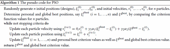
Let $\mathcal{X}=[u_1,v_1]\times \cdots \times [u_{p-1},v_{p-1}]$, when some of the parameters ${\text{β}}_1,\dots ,{\text{β}}_{p-1}$ are equal to zero. It follows from Lemma 1 of Schmidt (2019) that the two endpoints of the corresponding edges must be the support points of optimal design, and the number of support points is possibly over p. This means that we need to use some numerical algorithms to generate the R-optimal design, such as the commonly used particle swarm optimization (PSO) method, see Section 4.2 for details.

The following two examples illustrate the results in Theorem 3.1 and Remark 3.1, and exhibit the performance of different designs in terms of the Bonferroni confidence intervals and the relative efficiencies of designs. In Example 3.1 the first-order Poisson regression model with intercept will be considered, and the difference of the averaged Bonferroni confidence intervals derived by R- and D-optimal designs as well as the balanced design ${\xi }_b$ will be investigated by a numerical simulation. Example 3.2 considers the Poisson regression model with two covariants which was discussed in Schmidt (2019), and the relative efficiency of R-optimal designs will be compared with other designs. In both of the examples, the intensity function Q is given by $Q\left(\theta \right)=\exp \left(\theta \right)$ for $\theta \in \mathbb{R}$.

Example 3.1

Consider the first-order Poisson regression model with intercept and let $\mathcal{X}=[0,5]$. If we set $\text{β}=(6,-1{)}^{\mathrm{\top }}$ and $\text{β}=(1,1{)}^{\mathrm{\top }}$, the R- and D-optimal designs can be calculated numerically by Theorem 3.1 and Theorem 2 of Konstantinou et al. (2014). For example, under the R-optimality criterion with $\text{β}=(6,-1{)}^{\mathrm{\top }}$ we obtain $x_1^{\ast }=2.1886$ and ${\omega }_2^{\ast }=0.5431$ by solving the Equations (4(4) ${\omega }_j^{\ast }=\sqrt{\frac{s_{jj}}{p}},j=1,\dots ,p,$(4) ) and (6(6) $x_i-2\frac{Q\left(\mathit{f}\right(\mathit{a}{)}^{\mathrm{\top }}\text{β}-x_i)}{Q^{\mathrm{\prime }}\left(\mathit{f}\right(\mathit{a}{)}^{\mathrm{\top }}\text{β}-x_i)}[1-\sqrt{\frac{Q\left(\mathit{f}\right(\mathit{a}{)}^{\mathrm{\top }}\text{β}-x_i)}{Q\left(\mathit{f}\right(\mathit{a}{)}^{\mathrm{\top }}\text{β})}}\frac{s_{1,i+1}}{\sqrt{s_{11}{s}_{i+1,i+1}}}]=0.$(6) ). In Table 1, the results on optimal designs for both cases are reported. Furthermore, we carry out a simulation study in order to assess the difference of the Bonferroni confidence intervals derived by different designs. The averaged Bonferroni confidence intervals under different sample sizes are calculated by 10,000 simulation runs, which are shown in Table 1. We find from Table 1 that for both cases the coverage probabilities perform in a similar manner and much close to 0.95 as the sample size increases, and the width of the averaged Bonferroni confidence intervals obtained from R-optimal designs is narrower comparing with D-optimal designs and the balanced design ${\xi }_b$ when there exists a serious loss of R-efficiency.

Table 1. The simulation results obtained from the locally R-, D-optimal designs and the balanced design on $\mathcal{X}=[0,5]$ for the first-order Poisson regression model with intercept.

Sample size	Design	R-efficiency	BCI${}^{†}$	CP${}^{\text{‡}}$
Case A: ${\text{β}}_0=6,{\text{β}}_1=-1$
	${\xi }_R^{\ast }=\left\{\begin{array}{cc}0& 2.1886\\ 0.5431& 0.4569\end{array}\right\}$	1	$[5.9506,6.0491]$	0.9709
			$[-1.0209,-0.9792]$	0.9821
10	${\xi }_D^{\ast }=\left\{\begin{array}{cc}0& 2\\ 0.5& 0.5\end{array}\right\}$	0.9792	$[5.9485,6.0512]$	0.9803
			$[-1.0756,-0.9266]$	0.9783
	${\xi }_b=\left\{\begin{array}{cc}0& 5\\ 0.5& 0.5\end{array}\right\}$	0.3436	$[5.9482,6.0509]$	0.9790
			$[\mathbf{-}\mathbf{1.1357},\mathbf{-}\mathbf{0.8776}]$	0.9821
	${\xi }_R^{\ast }=\left\{\begin{array}{cc}0& 2.1886\\ 0.5431& 0.4569\end{array}\right\}$	1	$[5.9866,6.0134]$	0.9510
			$[-1.0209,-0.9792]$	0.9536
100	${\xi }_D^{\ast }=\left\{\begin{array}{cc}0& 2\\ 0.5& 0.5\end{array}\right\}$	0.9792	$[5.9860,6.0139]$	0.9538
			$[-1.0203,-0.9799]$	0.9523
	${\xi }_b=\left\{\begin{array}{cc}0& 5\\ 0.5& 0.5\end{array}\right\}$	0.3436	$[5.9860,6.0140]$	0.9540
			$[\mathbf{-}\mathbf{1.0351},\mathbf{-}\mathbf{0.9665}]$	0.9561
Case B: ${\text{β}}_0=1,{\text{β}}_1=1$
	${\xi }_R^{\ast }=\left\{\begin{array}{cc}2.4678& 5\\ 0.8234& 0.1766\end{array}\right\}$	1	$[0.7045,1.2904]$	0.9765
			$[0.9346,1.0660]$	0.9792
10	${\xi }_D^{\ast }=\left\{\begin{array}{cc}3& 5\\ 0.5& 0.5\end{array}\right\}$	0.5221	$[0.6404,1.3557]$	0.9800
			$[0.9258,1.0747]$	0.9792
	${\xi }_b=\left\{\begin{array}{cc}0& 5\\ 0.5& 0.5\end{array}\right\}$	0.0598	$[\mathbf{0.3139},\mathbf{1.6046}]$	0.9853
			$[\mathbf{0.8785},\mathbf{1.1375}]$	0.9813
	${\xi }_R^{\ast }=\left\{\begin{array}{cc}2.4678& 5\\ 0.8234& 0.1766\end{array}\right\}$	1	$[0.9205,1.0797]$	0.9532
			$[0.9821,1.0178]$	0.9547
100	${\xi }_D^{\ast }=\left\{\begin{array}{cc}3& 5\\ 0.5& 0.5\end{array}\right\}$	0.5221	$[0.9031,1.0976]$	0.9523
			$[0.9796,1.0202]$	0.9531
	${\xi }_b=\left\{\begin{array}{cc}0& 5\\ 0.5& 0.5\end{array}\right\}$	0.0598	$[\mathbf{0.8258},\mathbf{1.1671}]$	0.9621
			$[\mathbf{0.9664},\mathbf{1.0349}]$	0.9603

${}^{†}$ The abbreviation ‘BCI’ represents the Bonferroni confidence intervals of the parameters ${\text{β}}_0$ and ${\text{β}}_1$, where the first row under each design is the simulation results of ${\text{β}}_0$, and the second row is ${\text{β}}_1$.

${}^{\text{‡}}$ The abbreviation ‘CP’ represents the coverage probabilities of 95% confidence intervals for the parameters ${\text{β}}_0$ and ${\text{β}}_1$.

Example 3.2

Assume that the linear predictor in the considered Poisson regression model includes an intercept term. Let $\mathcal{X}=[0,5{]}^2$ and $\text{β}=(0,-1,-1{)}^{\mathrm{\top }}$. A numerical calculation yields immediately $x_1^{\ast }=x_2^{\ast }=2.1785$, ${\omega }_1^{\ast }={\omega }_2^{\ast }=0.3060$ and ${\omega }_3^{\ast }=0.3880$ by the Equations (4(4) ${\omega }_j^{\ast }=\sqrt{\frac{s_{jj}}{p}},j=1,\dots ,p,$(4) ) and (6(6) $x_i-2\frac{Q\left(\mathit{f}\right(\mathit{a}{)}^{\mathrm{\top }}\text{β}-x_i)}{Q^{\mathrm{\prime }}\left(\mathit{f}\right(\mathit{a}{)}^{\mathrm{\top }}\text{β}-x_i)}[1-\sqrt{\frac{Q\left(\mathit{f}\right(\mathit{a}{)}^{\mathrm{\top }}\text{β}-x_i)}{Q\left(\mathit{f}\right(\mathit{a}{)}^{\mathrm{\top }}\text{β})}}\frac{s_{1,i+1}}{\sqrt{s_{11}{s}_{i+1,i+1}}}]=0.$(6) ). The R-optimal design is given in Table 2. The PSO method was used to find the corresponding D-, R-, and A-optimal designs when $\text{β}=(0,-1,0{)}^{\mathrm{\top }}$. The resulting designs are listed in Table 2. In this case, we find that the endpoints $(0,0)$ and $(0,5)$ must be the support points of optimal designs. Figure 1 displays the plot of the function $\varphi (\mathit{x},\text{β})$ defined in (3(3) $\varphi (\mathit{x},\text{β})=Q\left(\mathit{f}\right(\mathit{x}{)}^{\mathrm{\top }}\text{β}\left)\mathit{f}\right(\mathit{x}{)}^{\mathrm{\top }}\mathit{M}({\xi }^{\ast },\text{β}{)}^{-1}\left(\sum _{j=1}^p\frac{{\mathit{e}}_{j,p}{\mathit{e}}_{j,p}^{\mathrm{\top }}}{{\mathit{e}}_{j,p}^{\mathrm{\top }}\mathit{M}({\xi }^{\ast },\text{β}{)}^{-1}{\mathit{e}}_{j,p}}\right)\mathit{M}({\xi }^{\ast },\text{β}{)}^{-1}\mathit{f}\left(\mathit{x}\right)⩽p$(3) ) for the cases $\text{β}=(0,-1,-1{)}^{\mathrm{\top }}$ and $\text{β}=(0,-1,0{)}^{\mathrm{\top }}$, which indicates that the function ϕ attains its maximum 3 at each support point.

Figure 1. Plot of the function ϕ in (3(3) $\varphi (\mathit{x},\text{β})=Q\left(\mathit{f}\right(\mathit{x}{)}^{\mathrm{\top }}\text{β}\left)\mathit{f}\right(\mathit{x}{)}^{\mathrm{\top }}\mathit{M}({\xi }^{\ast },\text{β}{)}^{-1}\left(\sum _{j=1}^p\frac{{\mathit{e}}_{j,p}{\mathit{e}}_{j,p}^{\mathrm{\top }}}{{\mathit{e}}_{j,p}^{\mathrm{\top }}\mathit{M}({\xi }^{\ast },\text{β}{)}^{-1}{\mathit{e}}_{j,p}}\right)\mathit{M}({\xi }^{\ast },\text{β}{)}^{-1}\mathit{f}\left(\mathit{x}\right)⩽p$(3) ) for the R-optimal design on $\mathcal{X}=[0,5{]}^2$ for the Poisson regression model discussed in Example 3.2: (a) for $\text{β}=(0,-1,-1{)}^{\mathrm{\top }}$ and (b) for $\text{β}=(0,-1,0{)}^{\mathrm{\top }}$.

Table 2. Comparison of R-optimal design with D- and A-optimal designs on $\mathcal{X}=[0,5{]}^2$ for the Poisson regression model discussed in Example 3.2.

			Efficiencies
$\text{β}$	Criterion	Optimal design	Eff${}_D(\xi {)}^{†}$	Eff${}_R\left(\xi \right)$	Eff${}_A(\xi {)}^{†}$
	D	${\xi }_D^{\ast }=\left\{\begin{array}{ccc}(2,0)& (0,2)& (0,0)\\ 1/3& 1/3& 1/3\end{array}\right\}$	1	0.9526	0.9856
$(0,-1,-1)$	R	${\xi }_R^{\ast }=\left\{\begin{array}{ccc}(2.1785,0)& (0,2.1785)& (0,0)\\ 0.3060& 0.3060& 0.3880\end{array}\right\}$	0.9886	1	0.9704
	A	${\xi }_A^{\ast }=\left\{\begin{array}{ccc}(2.2453,0)& (0,2.2453)& (0,0)\\ 0.3492& 0.3492& 0.3016\end{array}\right\}$	0.9884	0.9409	1
	D	${\xi }_D^{\ast }=\left\{\begin{array}{cccc}(1.8493,5)& (1.8493,0)& (0,5)& (0,0)\\ 0.3197& 0.3197& 0.1802& 0.1802\end{array}\right\}$	1	0.8454	0.7905
$(0,-1,0)$	R	${\xi }_R^{\ast }=\left\{\begin{array}{cccc}(1.9449,5)& (1.9449,0)& (0,5)& (0,0)\\ 0.1476& 0.1951& 0.2185& 0.4388\end{array}\right\}$	0.9622	1	0.8435
	A	${\xi }_A^{\ast }=\left\{\begin{array}{cccc}(2.1798,5)& (2.1798,0)& (0,5)& (0,0)\\ 0.1198& 0.4054& 0.0757& 0.3991\end{array}\right\}$	0.7717	0.6183	1

${}^{†}$The D- and A-efficiencies are defined as ${\mathrm{E}\mathrm{f}\mathrm{f}}_D\left(\xi \right)=\left\{\mathrm{d}\mathrm{e}\mathrm{t}\right(\mathit{M}(\xi ,\text{β})\left)/\mathrm{d}\mathrm{e}\mathrm{t}\right(\mathit{M}({\xi }^{\ast },\text{β})){\}}^{1/p}$ and ${\mathrm{E}\mathrm{f}\mathrm{f}}_A\left(\xi \right)=\mathrm{t}\mathrm{r}\left({\mathit{M}}^{-1}\right({\xi }^{\ast },\text{β}\left)\right)/\mathrm{t}\mathrm{r}\left({\mathit{M}}^{-1}\right(\xi ,\text{β}\left)\right)$, respectively, where $\mathrm{d}\mathrm{e}\mathrm{t}(\cdot )$ and $\mathrm{t}\mathrm{r}(\cdot )$ are the matrix determinant and trace functions.

To compare the performance of different designs, such as the common D- and A-optimality, we may calculate the related efficiency that usually defines the value of the criterion function for the optimal design relative to the value of the criterion function of a design and can thus take values between 0 and 1. For instance, the R-efficiency is defined as ${\mathrm{E}\mathrm{f}\mathrm{f}}_R\left(\xi \right)=\psi ({\xi }^{\ast },\text{β})/\psi (\xi ,\text{β})$. The results are summarized in Table 2. For the case $\text{β}=(0,-1,-1{)}^{\mathrm{\top }}$, all the designs have relatively high efficiencies regarding the other optimality criteria. This occurs primarily because the designs have a similar structure. For the case $\text{β}=(0,-1,0{)}^{\mathrm{\top }}$, we observe that the R-optimal design still has relatively high D- and A-efficiencies, but the A-optimal design has a large loss of R-efficiency.

Theorem 3.2

Let $\mathcal{X}=[0,\mathrm{\infty }{)}^{p-1}$ and let the assumptions (A1)–(A4) be satisfied for models with information matrices of the form (1(1) $\mathit{M}(\xi ,\text{β})={\int }_{\mathcal{X}}Q\left(\mathit{f}\right(\mathit{x}{)}^{\mathrm{\top }}\text{β}\left)\mathit{f}\right(\mathit{x}\left)\mathit{f}\right(\mathit{x}{)}^{\mathrm{\top }}\mathrm{d}\xi \left(\mathit{x}\right)=\sum _{i=1}^m{\omega }_{i}Q\left(\mathit{f}\right({\mathit{x}}_i{)}^{\mathrm{\top }}\text{β}\left)\mathit{f}\right({\mathit{x}}_i\left)\mathit{f}\right({\mathit{x}}_i{)}^{\mathrm{\top }},$(1) ). If ${\text{β}}_i<0$ for all $i=1,\dots ,p-1$, then the solutions $x_i^{\ast }$ and ${\omega }_i^{\ast }$ from the system of Equations (4(4) ${\omega }_j^{\ast }=\sqrt{\frac{s_{jj}}{p}},j=1,\dots ,p,$(4) ) and (6(6) $x_i-2\frac{Q\left(\mathit{f}\right(\mathit{a}{)}^{\mathrm{\top }}\text{β}-x_i)}{Q^{\mathrm{\prime }}\left(\mathit{f}\right(\mathit{a}{)}^{\mathrm{\top }}\text{β}-x_i)}[1-\sqrt{\frac{Q\left(\mathit{f}\right(\mathit{a}{)}^{\mathrm{\top }}\text{β}-x_i)}{Q\left(\mathit{f}\right(\mathit{a}{)}^{\mathrm{\top }}\text{β})}}\frac{s_{1,i+1}}{\sqrt{s_{11}{s}_{i+1,i+1}}}]=0.$(6) ) do not depend on the parameter vector $({\text{β}}_1,\dots ,{\text{β}}_{p-1}{)}^{\mathrm{\top }}$, that is, the R-optimal weights are unchanged for different $({\text{β}}_1,\dots ,{\text{β}}_{p-1}{)}^{\mathrm{\top }}$ when ${\text{β}}_0$ is fixed.

Remark 3.2

The optimal weights of saturated designs for L- and ${\mathrm{\Phi }}_k$-optimality criteria, except for D-optimality, depend on the parameters $({\text{β}}_1,\dots ,{\text{β}}_{p-1}{)}^{\mathrm{\top }}$ in the same settings of Theorem 3.2.

To further illustrate Theorem 3.2, we consider the proportional hazards regression models with two types of censoring. Under type I censoring with a fixed censoring time c the intensity function Q is given by $Q\left(\theta \right)=1-\exp (-c\exp (\theta \left)\right)$. For random censoring the intensity function $Q\left(\theta \right)$ equals to $1-[1-\exp (-c\exp \left(\theta \right)\left)\right]/[c\exp (\theta \left)\right]$ if the censoring times are assumed to follow a uniform distribution $U(0,c)$ (see Konstantinou et al., 2014). For both the above-mentioned intensity functions the variable θ belongs to $\mathbb{R}$.

Example 3.3

For the proportional hazards regression models with type I and random censoring Schmidt (2019) discussed the behaviour of c- and ${\mathrm{\Phi }}_k$-optimal designs for different parameter values. Their results are consistent with Remark 3.2. Analogous to Schmidt (2019), we investigate the performance of R-optimal designs on the design region $\mathcal{X}=[0,3{]}^{p-1}$ by comparing with a balanced design, say ${\xi }_b$, which is supported at all vertices of $\mathcal{X}$ with equal weights. First, the censoring time c as an unknown parameter should be determined previously, which is closely related to the amount of censoring q. Here q is also called the overall probability of censoring and given by $q=1-\sum {\omega }_{i}P(Y_j<C)$, in which $Y_i$ is the survival time and C is the censoring distribution (see Kalish & Harrington, 1988). For the two-covariate case, we choose c = 32 for type I censoring and c = 69 for random censoring such that q is, respectively, equal to 60% for $\text{β}=(3,-2.5,-2.5{)}^{\mathrm{\top }}$, 71% for $\text{β}=(3,-3,-3{)}^{\mathrm{\top }}$ and $75\mathrm{\%}$ for $\text{β}=(3,-4,-4{)}^{\mathrm{\top }}$ when the balanced design ${\xi }_b$ on $\mathcal{X}=[0,3{]}^2$ had been used. The R-optimal designs on $\mathcal{X}=[0,3{]}^2$ and R-efficiencies of ${\xi }_b$ are summarized in Table 3. We observe from Table 3 that the R-optimal designs shift the support points on the edges towards the vertex $(0,0{)}^{\mathrm{\top }}$ and the R-efficiencies of the balanced design ${\xi }_b$ decrease with increasing amounts of censoring. Note also that the R-efficiency of ${\xi }_b$ is quite low for these censoring scenarios. In addition, the R-optimal weights are the same for each model by Theorem 3.2.

Table 3. R-optimal designs on $\mathcal{X}=[0,3{]}^2$ for proportional hazards regression models for different $\text{β}$ and R-efficiencies of the balanced design ${\xi }_b$.

$\text{β}$	R-optimal design for type I censoring	Eff${}_R\left({\xi }_b\right)$
$(3,-2.5,-2.5)$	$\left\{\begin{array}{ccc}(2.4406,0)& (0,2.4406)& (0,0)\\ 0.2443& 0.2443& 0.5114\end{array}\right\}$	0.1986
$(3,-3,-3)$	$\left\{\begin{array}{ccc}(2.0338,0)& (0,2.0338)& (0,0)\\ 0.2443& 0.2443& 0.5114\end{array}\right\}$	0.0389
$(3,-4,-4)$	$\left\{\begin{array}{ccc}(1.5254,0)& (0,1.5254)& (0,0)\\ 0.2443& 0.2443& 0.5114\end{array}\right\}$	0.0004
	R-optimal design for random censoring
$(3,-2.5,-2.5)$	$\left\{\begin{array}{ccc}(2.4972,0)& (0,2.4972)& (0,0)\\ 0.2508& 0.2508& 0.4984\end{array}\right\}$	0.2307
$(3,-3,-3)$	$\left\{\begin{array}{ccc}(2.0810,0)& (0,2.0810)& (0,0)\\ 0.2508& 0.2508& 0.4984\end{array}\right\}$	0.0497
$(3,-4,-4)$	$\left\{\begin{array}{ccc}(1.5607,0)& (0,1.5607)& (0,0)\\ 0.2508& 0.2508& 0.4984\end{array}\right\}$	0.0005

4. R-optimal designs for models without intercept

In the present section we turn to discuss the multi-linear case without intercept, where the vector of the regressor functions is specified as $\mathit{f}=(x_1,\dots ,x_p{)}^{\mathrm{\top }}\in \mathcal{X}$, $p⩾2$, and the parameter vector is denoted by $\text{β}=({\text{β}}_1,\dots ,{\text{β}}_p{)}^{\mathrm{\top }}$. The regression model without an intercept is common and it usually arises from the physical characteristics of the variables measured. The design issue for this model has attracted considerable attention in the literature (see, e.g., Idais & Schwabe, 2021; Li et al., 2005 and the references cited there).

Let $\mathcal{X}=[u_1,v_1]\times \cdots \times [u_p,v_p]$. Then the support points of R-optimal designs are also at the edges of $\mathcal{X}$ by Theorem 2 in Schmidt (2019). Moreover, from the proof of Theorem 8 in Schmidt (2019) the support points of an R-optimal design ${\xi }^{\ast }$ must be given by $\mathit{a}-\left(x_1/{\text{β}}_1\right){\mathit{e}}_{1,p-1},\dots ,\mathit{a}-\left(x_p/{\text{β}}_p\right){\mathit{e}}_{p,p}$ and $\mathit{a}=(a_1,\dots ,a_p{)}^{\mathrm{\top }}$ with $a_i=v_i$ if ${\text{β}}_i>0$ and $a_i=u_i$ if ${\text{β}}_i<0$ for $i=1,\dots ,p$. As a result, the optimality condition for approximate designs in Theorem 2.1 can be simplified to verify whether it is satisfied at the boundary of the design region, i.e., the design ${\xi }^{\ast }$ is R-optimal if and only if (7) $h_i(x_i,{\xi }^{\ast })={\ell }_i(x_i,{\xi }^{\ast })-\frac{p}{Q({\mathit{a}}^{\mathrm{\top }}\text{β}+{\text{β}}_i(x_i-a_i\left)\right)}⩽0$(7) holds for all $x_i$, $i=1,\dots ,p$, where the function ${\ell }_i(x_i,{\xi }^{\ast })$ is given by ${\ell }_i(x_i,{\xi }^{\ast })=(\mathit{a}+(x_i-a_i\left){\mathit{e}}_{i,p}{)}^{\mathrm{\top }}\mathit{M}\right({\xi }^{\ast },\text{β}{)}^{-1}\left(\sum _{j=1}^p\frac{{\mathit{e}}_{j,p}{\mathit{e}}_{j,p}^{\mathrm{\top }}}{{\mathit{e}}_{j,p}^{\mathrm{\top }}\mathit{M}({\xi }^{\ast },\text{β}{)}^{-1}{\mathit{e}}_{j,p}}\right)\mathit{M}({\xi }^{\ast },\text{β}{)}^{-1}(\mathit{a}+(x_i-a_i){\mathit{e}}_{i,p}).$

4.1. Some theoretical results on saturated designs

In this subsection, we will provide two types of saturated R-optimal designs for the model considered by distinguishing whether the vertex $\mathit{a}$ is a support point. The first result reveals designs which include the support point $\mathit{a}$, where the condition $a_{\tau }\ne 0$, $\tau \in \{1,\dots ,p\}$, described in Theorem 4.1 is to guarantee the design ${\xi }_{\tau }^{\ast }$ in (9(9) ${\xi }_{\tau }^{\ast }=\left\{\begin{array}{ccccc}\mathit{a}-\left(x_1^{\ast }/{\text{β}}_1\right){\mathit{e}}_{1,p}& \cdots & \mathit{a}-\left(x_{\tau }^{\ast }/{\text{β}}_{\tau }\right){\mathit{e}}_{\tau ,p}& \cdots & \mathit{a}-\left(x_p^{\ast }/{\text{β}}_p\right){\mathit{e}}_{p,p}\\ {\omega }_1^{\ast }& \cdots & {\omega }_{\tau }^{\ast }& \cdots & {\omega }_p^{\ast }\end{array}\right\}$(9) ) with a non-singular information matrix.

Theorem 4.1

Let the assumptions (A1)–(A4) be satisfied for models with information matrices of the form (1(1) $\mathit{M}(\xi ,\text{β})={\int }_{\mathcal{X}}Q\left(\mathit{f}\right(\mathit{x}{)}^{\mathrm{\top }}\text{β}\left)\mathit{f}\right(\mathit{x}\left)\mathit{f}\right(\mathit{x}{)}^{\mathrm{\top }}\mathrm{d}\xi \left(\mathit{x}\right)=\sum _{i=1}^m{\omega }_{i}Q\left(\mathit{f}\right({\mathit{x}}_i{)}^{\mathrm{\top }}\text{β}\left)\mathit{f}\right({\mathit{x}}_i\left)\mathit{f}\right({\mathit{x}}_i{)}^{\mathrm{\top }},$(1) ) and without intercept. Let $s_{ij}$ $\left(i,j=1,\dots ,p\right)$ be the elements of the matrix $\mathit{S}$ in (5(5) $\mathit{S}={\left({\tilde{\mathit{X}}}^{-1}\right)}^{\mathrm{\top }}\left(\sum _{j=1}^p\frac{{\mathit{e}}_{j,p}{\mathit{e}}_{j,p}^{\mathrm{\top }}}{{\mathit{e}}_{j,p}^{\mathrm{\top }}\mathit{M}(\xi ,\text{β}{)}^{-1}{\mathit{e}}_{j,p}}\right){\tilde{\mathit{X}}}^{-1}.$(5) ) evaluated at a design of the form $\{\mathit{a}-(x_i/{\text{β}}_i){\mathit{e}}_{i,p};{\omega }_i{\}}_{i=1}^p$. For a given index τ $(\tau \in \{1,\dots ,p\left\}\right)$ with $a_{\tau }\ne 0$, if a solution exists, let $x_i^{\ast }\in (0,\mathrm{\infty })$ and the weights ${\omega }_i^{\ast }$ be the unique solutions of the common system of Equations (4(4) ${\omega }_j^{\ast }=\sqrt{\frac{s_{jj}}{p}},j=1,\dots ,p,$(4) ) and (8(8) $x_i-2\frac{Q({\mathit{a}}^{\mathrm{\top }}\text{β}-x_i)}{Q^{\mathrm{\prime }}({\mathit{a}}^{\mathrm{\top }}\text{β}-x_i)}[1-\sqrt{\frac{Q({\mathit{a}}^{\mathrm{\top }}\text{β}-x_i)}{Q\left({\mathit{a}}^{\mathrm{\top }}\text{β}\right)}}\frac{s_{\tau i}}{\sqrt{s_{\tau \tau }{s}_{ii}}}]=0$(8) ) given by (8) $x_i-2\frac{Q({\mathit{a}}^{\mathrm{\top }}\text{β}-x_i)}{Q^{\mathrm{\prime }}({\mathit{a}}^{\mathrm{\top }}\text{β}-x_i)}[1-\sqrt{\frac{Q({\mathit{a}}^{\mathrm{\top }}\text{β}-x_i)}{Q\left({\mathit{a}}^{\mathrm{\top }}\text{β}\right)}}\frac{s_{\tau i}}{\sqrt{s_{\tau \tau }{s}_{ii}}}]=0$(8) for all i $(\ne \tau )$. If $0<x_i^{\ast }⩽|{\text{β}}_i|(v_i-u_i)$ holds, then the design (9) ${\xi }_{\tau }^{\ast }=\left\{\begin{array}{ccccc}\mathit{a}-\left(x_1^{\ast }/{\text{β}}_1\right){\mathit{e}}_{1,p}& \cdots & \mathit{a}-\left(x_{\tau }^{\ast }/{\text{β}}_{\tau }\right){\mathit{e}}_{\tau ,p}& \cdots & \mathit{a}-\left(x_p^{\ast }/{\text{β}}_p\right){\mathit{e}}_{p,p}\\ {\omega }_1^{\ast }& \cdots & {\omega }_{\tau }^{\ast }& \cdots & {\omega }_p^{\ast }\end{array}\right\}$(9) with $x_{\tau }^{\ast }=0$ will be R-optimal on $\mathcal{X}$ provided that the condition $h_{\tau }(x_{\tau },{\xi }_{\tau }^{\ast })<0$ $\left(\mathrm{o}\mathrm{r}\varphi \right(\mathit{a}+(x_{\tau }-a_{\tau }){\mathit{e}}_{\tau ,p},\text{β})<p)$ for $x_{\tau }\in [u_{\tau },v_{\tau }]\mathrm{\setminus }\left\{a_{\tau }\right\}$ is satisfied, where $h_{\tau }(\cdot ,\cdot )$ is defined as in (7(7) $h_i(x_i,{\xi }^{\ast })={\ell }_i(x_i,{\xi }^{\ast })-\frac{p}{Q({\mathit{a}}^{\mathrm{\top }}\text{β}+{\text{β}}_i(x_i-a_i\left)\right)}⩽0$(7) ) and $\varphi (\cdot ,\cdot )$ as in (3(3) $\varphi (\mathit{x},\text{β})=Q\left(\mathit{f}\right(\mathit{x}{)}^{\mathrm{\top }}\text{β}\left)\mathit{f}\right(\mathit{x}{)}^{\mathrm{\top }}\mathit{M}({\xi }^{\ast },\text{β}{)}^{-1}\left(\sum _{j=1}^p\frac{{\mathit{e}}_{j,p}{\mathit{e}}_{j,p}^{\mathrm{\top }}}{{\mathit{e}}_{j,p}^{\mathrm{\top }}\mathit{M}({\xi }^{\ast },\text{β}{)}^{-1}{\mathit{e}}_{j,p}}\right)\mathit{M}({\xi }^{\ast },\text{β}{)}^{-1}\mathit{f}\left(\mathit{x}\right)⩽p$(3) ).

Example 4.1

Consider the Poisson regression model with two covariates and without intercept, where the design region is $\mathcal{X}=[0,5{]}^2$. To find the R-optimal design we first fix $\text{β}=(-0.5,0.5{)}^{\mathrm{\top }}$. According to Theorem 4.1 we can only specify $\tau =2$, i.e., $x_2^{\ast }=0$. By solving the common system of Equations (4(4) ${\omega }_j^{\ast }=\sqrt{\frac{s_{jj}}{p}},j=1,\dots ,p,$(4) ) and (10(10) $x_i-2\frac{Q({\mathit{a}}^{\mathrm{\top }}\text{β}-x_i)}{Q^{\mathrm{\prime }}({\mathit{a}}^{\mathrm{\top }}\text{β}-x_i)}[\frac{1}{1-{\mathit{z}}^{\mathrm{\top }}{\mathbf{1}}_p}\sum _{j=1}^p\frac{z_j\sqrt{Q({\mathit{a}}^{\mathrm{\top }}\text{β}-x_i)}}{\sqrt{Q({\mathit{a}}^{\mathrm{\top }}\text{β}-x_j)}}\frac{s_{ji}}{\sqrt{s_{ii}{s}_{jj}}}+1]=0$(10) ) we obtain $x_1^{\ast }=2.1886$ and the design ${\xi }_2^{\ast }$ is of the form ${\xi }_2^{\ast }=\left\{\begin{array}{cc}(4.3772,5)& (0,5)\\ 0.4569& 0.5431\end{array}\right\}.$It is easily verified that the condition $h_2(x_2,{\xi }_2^{\ast })<0$ is satisfied for $x_2\in [0,5)$ and the design ${\xi }_2^{\ast }$ is then R-optimal (see also Figure 2(a)). If we choose $\text{β}=(1,1{)}^{\mathrm{\top }}$, however, it follows from Theorem 4.1 that the designs ${\xi }_1^{\ast }$ and ${\xi }_2^{\ast }$ are given by ${\xi }_1^{\ast }=\left\{\begin{array}{cc}(2.4678,5)& (5,5)\\ 0.8234& 0.1766\end{array}\right\},{\xi }_2^{\ast }=\left\{\begin{array}{cc}(5,2.4678)& (0,5)\\ 0.8234& 0.1766\end{array}\right\},$respectively. In this case, the conditions $h_i(x_i,{\xi }_i^{\ast })<0$, i = 1, 2, are not satisfied, which means that both designs are not R-optimal. Accordingly, finding a saturated R-optimal design for this model that does not contain the support point $\mathit{a}$ may be an alternative scheme. This type of R-optimal design will be elaborated in Theorem 4.2.

Figure 2. Plots of the functions ϕ in (3(3) $\varphi (\mathit{x},\text{β})=Q\left(\mathit{f}\right(\mathit{x}{)}^{\mathrm{\top }}\text{β}\left)\mathit{f}\right(\mathit{x}{)}^{\mathrm{\top }}\mathit{M}({\xi }^{\ast },\text{β}{)}^{-1}\left(\sum _{j=1}^p\frac{{\mathit{e}}_{j,p}{\mathit{e}}_{j,p}^{\mathrm{\top }}}{{\mathit{e}}_{j,p}^{\mathrm{\top }}\mathit{M}({\xi }^{\ast },\text{β}{)}^{-1}{\mathit{e}}_{j,p}}\right)\mathit{M}({\xi }^{\ast },\text{β}{)}^{-1}\mathit{f}\left(\mathit{x}\right)⩽p$(3) ) for the R-optimal designs on $\mathcal{X}=[0,5{]}^2$ for the Poisson regression models discussed in Examples 4.1 and 4.2: (a) for $\text{β}=(-0.5,0.5{)}^{\mathrm{\top }}$ and (b) for $\text{β}=(1,1{)}^{\mathrm{\top }}$.

Theorem 4.2

Let the assumptions (A1)–(A4) be satisfied for models with information matrices of the form (1(1) $\mathit{M}(\xi ,\text{β})={\int }_{\mathcal{X}}Q\left(\mathit{f}\right(\mathit{x}{)}^{\mathrm{\top }}\text{β}\left)\mathit{f}\right(\mathit{x}\left)\mathit{f}\right(\mathit{x}{)}^{\mathrm{\top }}\mathrm{d}\xi \left(\mathit{x}\right)=\sum _{i=1}^m{\omega }_{i}Q\left(\mathit{f}\right({\mathit{x}}_i{)}^{\mathrm{\top }}\text{β}\left)\mathit{f}\right({\mathit{x}}_i\left)\mathit{f}\right({\mathit{x}}_i{)}^{\mathrm{\top }},$(1) ) and without intercept. Let $s_{ij}$ $\left(i,j=1,\dots ,p\right)$ be the elements of the matrix $\mathit{S}$ in (5(5) $\mathit{S}={\left({\tilde{\mathit{X}}}^{-1}\right)}^{\mathrm{\top }}\left(\sum _{j=1}^p\frac{{\mathit{e}}_{j,p}{\mathit{e}}_{j,p}^{\mathrm{\top }}}{{\mathit{e}}_{j,p}^{\mathrm{\top }}\mathit{M}(\xi ,\text{β}{)}^{-1}{\mathit{e}}_{j,p}}\right){\tilde{\mathit{X}}}^{-1}.$(5) ) evaluated at a design of the form $\{\mathit{a}-(x_i/{\text{β}}_i){\mathit{e}}_{i,p};{\omega }_i{\}}_{i=1}^p$. If a solution exists, let $x_i^{\ast }\in (0,\mathrm{\infty })$ and the weights ${\omega }_i^{\ast }$ be the unique solutions of the common system of Equations (4(4) ${\omega }_j^{\ast }=\sqrt{\frac{s_{jj}}{p}},j=1,\dots ,p,$(4) ) and (10(10) $x_i-2\frac{Q({\mathit{a}}^{\mathrm{\top }}\text{β}-x_i)}{Q^{\mathrm{\prime }}({\mathit{a}}^{\mathrm{\top }}\text{β}-x_i)}[\frac{1}{1-{\mathit{z}}^{\mathrm{\top }}{\mathbf{1}}_p}\sum _{j=1}^p\frac{z_j\sqrt{Q({\mathit{a}}^{\mathrm{\top }}\text{β}-x_i)}}{\sqrt{Q({\mathit{a}}^{\mathrm{\top }}\text{β}-x_j)}}\frac{s_{ji}}{\sqrt{s_{ii}{s}_{jj}}}+1]=0$(10) ) given by (10) $x_i-2\frac{Q({\mathit{a}}^{\mathrm{\top }}\text{β}-x_i)}{Q^{\mathrm{\prime }}({\mathit{a}}^{\mathrm{\top }}\text{β}-x_i)}[\frac{1}{1-{\mathit{z}}^{\mathrm{\top }}{\mathbf{1}}_p}\sum _{j=1}^p\frac{z_j\sqrt{Q({\mathit{a}}^{\mathrm{\top }}\text{β}-x_i)}}{\sqrt{Q({\mathit{a}}^{\mathrm{\top }}\text{β}-x_j)}}\frac{s_{ji}}{\sqrt{s_{ii}{s}_{jj}}}+1]=0$(10) for all i, where $\mathit{z}=(z_1,\dots ,z_p{)}^{\mathrm{\top }}$ with $z_j=a_j{\text{β}}_j/x_j$, ${\mathbf{1}}_p=(1,\dots ,1{)}^{\mathrm{\top }}\in {\mathbb{R}}^p$. If $0<x_i^{\ast }⩽|{\text{β}}_i|(v_i-u_i)$ holds, then the design (11) ${\xi }^{\ast }=\left\{\begin{array}{ccc}\mathit{a}-\left(x_1^{\ast }/{\text{β}}_1\right){\mathit{e}}_{1,p}& \cdots & \mathit{a}-\left(x_p^{\ast }/{\text{β}}_p\right){\mathit{e}}_{p,p}\\ {\omega }_1^{\ast }& \cdots & {\omega }_p^{\ast }\end{array}\right\}$(11) will be R-optimal on $\mathcal{X}$ provided that the condition $h_i(a_i,{\xi }^{\ast })<0$ $\left(\mathrm{o}\mathrm{r}\varphi \right(\mathit{a},\text{β})<p)$ is satisfied.

Example 4.2

Consider the same model given in Example 4.1. Here we consider $\text{β}=(1,1{)}^{\mathrm{\top }}$. The common system of Equations (4(4) ${\omega }_j^{\ast }=\sqrt{\frac{s_{jj}}{p}},j=1,\dots ,p,$(4) ) and (10(10) $x_i-2\frac{Q({\mathit{a}}^{\mathrm{\top }}\text{β}-x_i)}{Q^{\mathrm{\prime }}({\mathit{a}}^{\mathrm{\top }}\text{β}-x_i)}[\frac{1}{1-{\mathit{z}}^{\mathrm{\top }}{\mathbf{1}}_p}\sum _{j=1}^p\frac{z_j\sqrt{Q({\mathit{a}}^{\mathrm{\top }}\text{β}-x_i)}}{\sqrt{Q({\mathit{a}}^{\mathrm{\top }}\text{β}-x_j)}}\frac{s_{ji}}{\sqrt{s_{ii}{s}_{jj}}}+1]=0$(10) ) has the solutions $x_1^{\ast }=x_2^{\ast }=1.8755$ and ${\omega }_1^{\ast }={\omega }_2^{\ast }=0.5$. Then the design ${\xi }^{\ast }=\left\{\begin{array}{cc}(3.1245,5)& (5,3.1245)\\ 0.5& 0.5\end{array}\right\}$is R-optimal due to $\varphi (\mathit{a},\text{β})<2$ (see also Figure 2(b)).

Corollary 4.1

Let $\mathcal{X}=[0,\mathrm{\infty }{)}^p$ and let the assumptions (A1)–(A4) be satisfied for models with information matrices of the form (1(1) $\mathit{M}(\xi ,\text{β})={\int }_{\mathcal{X}}Q\left(\mathit{f}\right(\mathit{x}{)}^{\mathrm{\top }}\text{β}\left)\mathit{f}\right(\mathit{x}\left)\mathit{f}\right(\mathit{x}{)}^{\mathrm{\top }}\mathrm{d}\xi \left(\mathit{x}\right)=\sum _{i=1}^m{\omega }_{i}Q\left(\mathit{f}\right({\mathit{x}}_i{)}^{\mathrm{\top }}\text{β}\left)\mathit{f}\right({\mathit{x}}_i\left)\mathit{f}\right({\mathit{x}}_i{)}^{\mathrm{\top }},$(1) ) and without intercept. Then the following design ${\xi }^{\ast }$ is R-optimal for each ${\text{β}}_i<0$, $i=1,\dots ,p$, (12) ${\xi }^{\ast }=\left\{\begin{array}{ccc}-\left({\psi }^{-1}\right(0\left)/{\text{β}}_1\right){\mathit{e}}_{1,p}& \cdots & -\left({\psi }^{-1}\right(0\left)/{\text{β}}_p\right){\mathit{e}}_{p,p}\\ 1/p& \cdots & 1/p\end{array}\right\},$(12) where the function $\psi (\cdot )$ is defined as $\psi \left(x\right)=x-2Q(-x)/Q^{\mathrm{\prime }}(-x)$ for x>0.

Remark 4.1

It is worthwhile mentioning that the design (12(12) ${\xi }^{\ast }=\left\{\begin{array}{ccc}-\left({\psi }^{-1}\right(0\left)/{\text{β}}_1\right){\mathit{e}}_{1,p}& \cdots & -\left({\psi }^{-1}\right(0\left)/{\text{β}}_p\right){\mathit{e}}_{p,p}\\ 1/p& \cdots & 1/p\end{array}\right\},$(12) ) shown in Corollary 4.1 is also D- and A-optimal.

Remark 4.2

For the case of p = 1, the one point design ${\xi }^{\ast }=\{a;1\}$ that simultaneously satisfies the additional conditions in Theorem 4.1 is saturated R-optimal. However, if the design ${\xi }^{\ast }=\{a;1\}$ is not R-optimal, the proposed method in Theorem 4.2 can be used to search for a saturated R-optimal design.

4.2. PSO-generated R-optimal designs

Only finding saturated designs may not be enough for determining the R-optimality of a design in the design class Ξ, since the optimal designs depend on the unknown parameters. For example, let $\text{β}=(0.5,0.5{)}^{\mathrm{\top }}$ for the Poisson regression model discussed in Example 4.1. The R-optimal design (see Figure 3) is then given by ${\xi }^{\ast }=\left\{\begin{array}{ccc}(1.4321,5)& (5,1.4321)& (5,5)\\ 0.4666& 0.4666& 0.0668\end{array}\right\}.$This means that the number of support points of R-optimal designs for models without intercept may exceed the number of regression parameters. Thereby, the aforementioned method by solving equations is unable to determine an R-optimal design in Ξ and we require an effective algorithm to generate an R-optimal design. Here we employ the PSO algorithm to find optimal designs for the models under consideration and a pseudo code of PSO is described as below.

Figure 3. Plot of the function ϕ in (3(3) $\varphi (\mathit{x},\text{β})=Q\left(\mathit{f}\right(\mathit{x}{)}^{\mathrm{\top }}\text{β}\left)\mathit{f}\right(\mathit{x}{)}^{\mathrm{\top }}\mathit{M}({\xi }^{\ast },\text{β}{)}^{-1}\left(\sum _{j=1}^p\frac{{\mathit{e}}_{j,p}{\mathit{e}}_{j,p}^{\mathrm{\top }}}{{\mathit{e}}_{j,p}^{\mathrm{\top }}\mathit{M}({\xi }^{\ast },\text{β}{)}^{-1}{\mathit{e}}_{j,p}}\right)\mathit{M}({\xi }^{\ast },\text{β}{)}^{-1}\mathit{f}\left(\mathit{x}\right)⩽p$(3) ) for the R-optimal design on $\mathcal{X}=[0,5{]}^2$ for $\text{β}=(0.5,0.5{)}^{\mathrm{\top }}$ in the Poisson regression model without intercept.

In Section 4.2, the support points of each position ${\xi }_i$ must be given by $\mathit{a}-\left(x_1/{\text{β}}_1\right){\mathit{e}}_{1,p-1},\dots ,\mathit{a}-\left(x_p/{\text{β}}_p\right){\mathit{e}}_{p,p}$ and $\mathit{a}$.

The index t is equal to $0,1,\dots$, and two criteria can be used to end iteration, achieving a maximum number of iterations or verifying whether the equivalence condition attains a pre-specified threshold.

The notations $v_i^{\left(t\right)}$ and ${\xi }_i^{\left(t\right)}$ are, respectively, the current velocity and position for the ith particle. ${\theta }_t$ is the inertia weight that modulates the influence of the former velocity, which can be a constant or a decreasing function with values between 0 and 1. ${\alpha }_1$ and ${\alpha }_2$ are both random variables from $U(0,1)$. ${\gamma }_1$ and ${\gamma }_2$ are two constants reflecting the cognitive learning level and social learning level, respectively.

Example 4.3

Consider the proportional hazards regression models with three covariates, in which the linear predictor does not include an intercept term. Let $\mathcal{X}=[0,3{]}^3$ and $\text{β}=(-2.5,0.5,0.5{)}^{\mathrm{\top }}$. In order to assess the effect of the amount of censoring q on R-optimal designs, we adjust the censoring time c to achieve overall censoring probabilities of 20%, 40%, 60% and 80% for the balanced design ${\xi }_b$. For instance, we choose c = 60 for type I censoring and c = 133 for random censoring when q = 0.4. In this example, the PSO algorithm with 150 particles and 100 iterations is able to find the R-optimal design with the required accuracy, which can be implemented by $\mathsf{R}$ software in less than 20 seconds on a standard PC. Table 4 summarizes the numerical results, including R-efficiencies of the balanced design ${\xi }_b$ and the amount of censoring $q^{\ast }$ under the corresponding R-optimal design. Some of the points are clear from the numerical results.

• For the three-covariate case, the support points of R-optimal designs for type I censoring and random censoring exceed the number of parameters.

• With increasing amounts of censoring, the R-optimal designs shift the support point on the edge $(x_1,3,3{)}^{\mathrm{\top }}$ towards the vertex $\mathit{a}=(0,3,3{)}^{\mathrm{\top }}$, and the R-efficiency of the balanced design ${\xi }_b$ is reduced gradually.

• The overall probability of censoring $q^{\ast }$ under the R-optimal design is less than for the balanced design ${\xi }_b$.

Table 4. The locally R-optimal designs on $\mathcal{X}=[0,3{]}^3$ for $\text{β}=(-2.5,0.5,0.5{)}^{\mathrm{\top }}$ in the proportional hazards regression models, the R-efficiencies of the balanced design ${\xi }_b$ and the overall probability of censoring under the R-optimal design.

q	R-optimal design for type I censoring	Eff${}_R\left({\xi }_b\right)$	$q^{\ast }$
0.2	$\left\{\begin{array}{cccc}(3,3,3)& (0,0,3)& (0,3,0)& (0,3,3)\\ 0.2071& 0.3053& 0.3053& 0.1823\end{array}\right\}$	0.6286	0.0029
0.4	$\left\{\begin{array}{cccc}(2.6970,3,3)& (0,0,3)& (0,3,0)& (0,3,3)\\ 0.2200& 0.3032& 0.3032& 0.1736\end{array}\right\}$	0.2170	0.0525
0.6	$\left\{\begin{array}{cccc}(1.2854,3,3)& (0,0,3)& (0,3,0)& (0,3,3)\\ 0.2564& 0.2943& 0.2943& 0.1550\end{array}\right\}$	0.0193	0.2309
0.8	$\left\{\begin{array}{cccc}(1.0354,3,3)& (0,0,3)& (0,3,0)& (0,3,3)\\ 0.2762& 0.2887& 0.2887& 0.1464\end{array}\right\}$	0.0122	0.6477
	R-optimal design for random censoring
0.2	$\left\{\begin{array}{cccc}(3,3,3)& (0,0,3)& (0,3,0)& (0,3,3)\\ 0.2112& 0.3046& 0.3046& 0.1796\end{array}\right\}$	0.6941	0.0192
0.4	$\left\{\begin{array}{cccc}(2.7596,3,3)& (0,0,3)& (0,3,0)& (0,3,3)\\ 0.2274& 0.3019& 0.3019& 0.1688\end{array}\right\}$	0.2367	0.0796
0.6	$\left\{\begin{array}{cccc}(1.4216,3,3)& (0,0,3)& (0,3,0)& (0,3,3)\\ 0.2538& 0.2946& 0.2946& 0.1570\end{array}\right\}$	0.0244	0.2541
0.8	$\left\{\begin{array}{cccc}(1.0763,3,3)& (0,0,3)& (0,3,0)& (0,3,3)\\ 0.2735& 0.2882& 0.2882& 0.1501\end{array}\right\}$	0.0132	0.6387

5. Discussion

The present paper investigates the construction of locally R-optimal designs for a large class of nonlinear multiple regression models. For the case of models with intercept, the R-optimal designs on a rectangular design region can be determined by utilizing the similar arguments in Schmidt (2019) but finding its optimal weight is different. We notice that the structure of the R-optimal designs is similar to those criteria reported in Schmidt (2019), especially in terms of the location of support points. For the case of models without intercept, however, with the same method we can determine the saturated R-optimal designs only from two design subclasses addressed in Section 4.1. Moreover, the PSO algorithm has been used to generate non-saturated R-optimal designs for both cases. Some conditions in Theorems 3.1, 4.1 and 4.2 are required, which ensure that the support points are located within the design region. If these conditions are not satisfied, optimal designs may then be having more support points. In addition, a nonlinear system of equations must be solved numerically in order to search for the saturated R-optimal designs. Although the existence of the solution to these equations is not proved theoretically, the numerical exploration shows that the solution in all considered examples always exists.

It is worthwhile mentioning that the locally optimal designs discussed so far are derived for a given value of the model parameter vector $\text{β}$. One might choose such a value of $\text{β}$ from an initial guess or estimation when some historical observations can be obtained. It might be of interest to study how the design will be affected by wrongly specified parameters. For illustration, we consider the locally R-optimal designs for the first-order Poisson regression models with an intercept on the design region $\mathcal{X}=[0,5{]}^{p-1}$ for p = 2, 3, 4, respectively. In specific, we assume that the true parameter vector is $\text{β}=(0,-1{)}^{\mathrm{\top }}$ for p = 2, $\text{β}=(0,-1,-1{)}^{\mathrm{\top }}$ for p = 3, and $\text{β}=(0,-1,-1,-1{)}^{\mathrm{\top }}$ for p = 4. We generate the locally R-optimal designs for various misspecified values of $\text{β}$, and calculate their R-efficiencies with respect to the locally R-optimal design for the true parameter vector for each p = 2, 3, 4, which are shown in Table 5. It is observed from Table 5 that the efficiency of the locally R-optimal design for the misspecified value of $\text{β}$ decreases as the value of $\text{β}$ diverges from its true value, and the loss of R-efficiency is disastrous when the difference between the true value and the misspecified value of $\text{β}$ is relatively serious. Numerical results with other examples yield similar conclusions, which are not reported here for the sake of saving space.

Table 5. The R-efficiencies of the locally R-optimal designs on $\mathcal{X}=[0,5{]}^{p-1}$ for various misspecified $\text{β}$ for the first-order Poisson regression models with intercept.

p = 2		p = 3		p = 4
$\text{β}$	Eff${}_R\left(\xi \right)$	$\text{β}$	Eff${}_R\left(\xi \right)$	$\text{β}$	Eff${}_R\left(\xi \right)$
$(0,-0.5)$	0.6376	$(0,-0.5,-0.5)$	0.4091	$(0,-0.5,-0.5,-0.5)$	0.2649
$(0,-0.8)$	0.9467	$(0,-0.8,-0.8)$	0.8970	$(0,-0.8,-0.8,-0.8)$	0.8519
$(0,-1.0)$	1	$(0,-1.0,-1.0)$	1	$(0,-1.0,-1.0,-1.0)$	1
$(0,-1.2)$	0.9588	$(0,-1.2,-1.2)$	0.9200	$(0,-1.2,-1.2,-1.2)$	0.8816
$(0,-1.5)$	0.7990	$(0,-1.5,-1.5)$	0.6409	$(0,-1.5,-1.5,-1.5)$	0.5132
$(0,-2.0)$	0.4854	$(0,-2.0,-2.0)$	0.2384	$(0,-2.0,-2.0,-2.0)$	0.1171

To overcome the parameter dependence of the locally optimal design, a commonly used approach to the computation of locally optimal designs is weighted designs (see, e.g., Atkinson et al., 2007, Chap. 18), where a prior distribution for $\text{β}$, which may be either discrete or continuous, is assumed in advance. Another method is the computation of maximin efficient designs, i.e., maximizing the minimal efficiency with respect to the parameters (see Dette, 1997; Konstantinou et al., 2014).

Disclosure statement

No potential conflict of interest was reported by the author(s).

Additional information

Funding

Lei He's work is supported by the National Natural Science Foundation of China [Grant Number 12101013] and the Natural Science Foundation of Anhui Province [Grant Number 2008085QA15]. Rong-Xian Yue's work is supported by the National Natural Science Foundation of China [Grant Numbers 11971318, 11871143].

Appendix

Proof

Proof of Theorem 2.1

Let ${\mathit{f}}_{\text{β}}\left(\mathit{x}\right)=\sqrt{Q\left(\mathit{f}\right(\mathit{x}{)}^{\mathrm{\top }}\text{β})}\mathit{f}\left(\mathit{x}\right)$. The Fisher information matrix of approximate design ξ given by (1(1) $\mathit{M}(\xi ,\text{β})={\int }_{\mathcal{X}}Q\left(\mathit{f}\right(\mathit{x}{)}^{\mathrm{\top }}\text{β}\left)\mathit{f}\right(\mathit{x}\left)\mathit{f}\right(\mathit{x}{)}^{\mathrm{\top }}\mathrm{d}\xi \left(\mathit{x}\right)=\sum _{i=1}^m{\omega }_{i}Q\left(\mathit{f}\right({\mathit{x}}_i{)}^{\mathrm{\top }}\text{β}\left)\mathit{f}\right({\mathit{x}}_i\left)\mathit{f}\right({\mathit{x}}_i{)}^{\mathrm{\top }},$(1) ) can then be written as $\mathit{M}(\xi ,\text{β})={\int }_{\mathcal{X}}{\mathit{f}}_{\text{β}}\left(\mathit{x}\right){\mathit{f}}_{\text{β}}\left(\mathit{x}{)}^{\mathrm{\top }}\mathrm{d}\xi \right(\mathit{x}).$For any designs $\xi ,\overline{\xi }\in \mathrm{\Xi }$ and $\alpha \in (0,1)$, define ${\xi }_{\alpha }=(1-\alpha )\xi +\alpha \overline{\xi }$. We have $\mathit{M}({\xi }_{\alpha },\text{β})=(1-\alpha )\mathit{M}(\xi ,\text{β})+\alpha \mathit{M}(\overline{\xi },\text{β})$ and $\begin{array}{rl}\frac{\mathrm{\partial }\psi ({\xi }_{\alpha },\text{β})}{\mathrm{\partial }\alpha }& =\frac{\mathrm{\partial }}{\mathrm{\partial }\alpha }\left[\prod _{j=1}^p{\mathit{e}}_{j,p}^{\mathrm{\top }}{\mathit{M}}^{-1}\right({\xi }_{\alpha },\text{β}\left){\mathit{e}}_{j,p}\right]\\ & =\sum _{j=1}^p\left(\prod _{\begin{array}{c}i=1\\ i\ne j\end{array}}^p{\mathit{e}}_{i,p}^{\mathrm{\top }}{\mathit{M}}^{-1}\right({\xi }_{\alpha },\text{β}\left){\mathit{e}}_{i,p}\right)\frac{\mathrm{\partial }}{\mathrm{\partial }\alpha }\left({\mathit{e}}_{j,p}^{\mathrm{\top }}{\mathit{M}}^{-1}\right({\xi }_{\alpha },\text{β}\left){\mathit{e}}_{j,p}\right),\end{array}$where $\frac{\mathrm{\partial }}{\mathrm{\partial }\alpha }\left({\mathit{e}}_{j,p}^{\mathrm{\top }}{\mathit{M}}^{-1}\right({\xi }_{\alpha },\text{β}\left){\mathit{e}}_{j,p}\right)={\mathit{e}}_{j,p}^{\mathrm{\top }}\left[{\mathit{M}}^{-1}\right({\xi }_{\alpha },\text{β}\left)\left(\mathit{M}\right(\xi ,\text{β})-\mathit{M}(\overline{\xi },\text{β}\left)\right){\mathit{M}}^{-1}\right({\xi }_{\alpha },\text{β}\left)\right]{\mathit{e}}_{j,p}.$The directional derivative of ψ at ξ in the direction of $\overline{\xi }$, denoted by ${\mathrm{\nabla }}_{\psi }(\xi ,\overline{\xi })$, is then given by $\begin{array}{rl}{\mathrm{\nabla }}_{\psi }(\xi ,\overline{\xi })& =\underset{\alpha \to 0^{+}}{lim}\frac{\mathrm{\partial }\psi ({\xi }_{\alpha },\text{β})}{\mathrm{\partial }\alpha }\\ & =\sum _{j=1}^p\frac{\psi \left(\xi \right)}{{\mathit{e}}_{j,p}^{\mathrm{\top }}{\mathit{M}}^{-1}(\xi ,\text{β}){\mathit{e}}_{j,p}}{\mathit{e}}_{j,p}^{\mathrm{\top }}\left[{\mathit{M}}^{-1}\right(\xi ,\text{β}\left)\left(\mathit{M}\right(\xi ,\text{β})-\mathit{M}(\overline{\xi },\text{β}\left)\right){\mathit{M}}^{-1}\right(\xi ,\text{β}\left)\right]{\mathit{e}}_{j,p}\\ & =\psi \left(\xi \right)\sum _{j=1}^p(1-\frac{{\mathit{e}}_{j,p}^{\mathrm{\top }}{\mathit{M}}^{-1}(\xi ,\text{β})\mathit{M}(\overline{\xi },\text{β}){\mathit{M}}^{-1}(\xi ,\text{β}){\mathit{e}}_{j,p}}{{\mathit{e}}_{j,p}^{\mathrm{\top }}{\mathit{M}}^{-1}(\xi ,\text{β}){\mathit{e}}_{j,p}})\\ & =\psi \left(\xi \right)(p-\mathrm{t}\mathrm{r}\left\{{\mathit{M}}^{-1}\right(\xi ,\text{β}\left)\mathit{M}\right(\overline{\xi },\text{β}\left){\mathit{M}}^{-1}\right(\xi ,\text{β}\left)\sum _{j=1}^q\frac{{\mathit{e}}_{j,p}{\mathit{e}}_{j,p}^{\mathrm{\top }}}{{\mathit{e}}_{j,p}^{\mathrm{\top }}{\mathit{M}}^{-1}(\xi ,\text{β}){\mathit{e}}_{j,p}}\right\}).\end{array}$Note that the directional derivative ${\mathrm{\nabla }}_{\psi }(\xi ,\overline{\xi })$ is linear in $\overline{\xi }$ for any fixed $\xi \in \mathrm{\Xi }$, i.e., ${\mathrm{\nabla }}_{\psi }(\xi ,\overline{\xi })={\int }_{\mathcal{X}}{\mathrm{\nabla }}_{\psi }(\xi ,{\delta }_{\mathit{x}})\mathrm{d}\overline{\xi }\left(\mathit{x}\right),$where ${\delta }_{\mathit{x}}$ is the Dirac measure at $\mathit{x}$. Following Whittle (1973), the design ${\xi }^{\ast }\in \mathrm{\Xi }$ is R-optimal if and only if $\underset{\mathit{x}\in \mathcal{X}}{inf}{\mathrm{\nabla }}_{\psi }(\xi ,{\delta }_{\mathit{x}})=0$. As a consequence the assertion of Theorem 2.1 follows.

Proof

Proof of Theorem 3.2

From Theorem 3.1, R-optimal design on $\mathcal{X}=[0,\mathrm{\infty }{)}^{p-1}$ for ${\text{β}}_i<0$, $i=1,\dots ,p-1$, has the following form (A1) $\xi =\left\{\begin{array}{cccc}-\left(x_1/{\text{β}}_1\right){\mathit{e}}_{1,p-1}& \cdots & -\left(x_{p-1}/{\text{β}}_{p-1}\right){\mathit{e}}_{p-1,p-1}& {\mathbf{0}}_{p-1}\\ {\omega }_1& \cdots & {\omega }_{p-1}& {\omega }_p\end{array}\right\},$(A1) where ${\mathbf{0}}_{p-1}$ is a vector of $(p-1)$ 0's, $x_i$ and ${\omega }_i$, $i=1,\dots ,p-1$, can be determined by the common system of Equations (4(4) ${\omega }_j^{\ast }=\sqrt{\frac{s_{jj}}{p}},j=1,\dots ,p,$(4) ) and (6(6) $x_i-2\frac{Q\left(\mathit{f}\right(\mathit{a}{)}^{\mathrm{\top }}\text{β}-x_i)}{Q^{\mathrm{\prime }}\left(\mathit{f}\right(\mathit{a}{)}^{\mathrm{\top }}\text{β}-x_i)}[1-\sqrt{\frac{Q\left(\mathit{f}\right(\mathit{a}{)}^{\mathrm{\top }}\text{β}-x_i)}{Q\left(\mathit{f}\right(\mathit{a}{)}^{\mathrm{\top }}\text{β})}}\frac{s_{1,i+1}}{\sqrt{s_{11}{s}_{i+1,i+1}}}]=0.$(6) ) for convenience. We denote $Q_i=Q({\text{β}}_0-x_i)$ for $i=1,\dots ,p-1$ and $Q_p=Q\left({\text{β}}_0\right)$ according to the support points of the design (A1(A1) $\xi =\left\{\begin{array}{cccc}-\left(x_1/{\text{β}}_1\right){\mathit{e}}_{1,p-1}& \cdots & -\left(x_{p-1}/{\text{β}}_{p-1}\right){\mathit{e}}_{p-1,p-1}& {\mathbf{0}}_{p-1}\\ {\omega }_1& \cdots & {\omega }_{p-1}& {\omega }_p\end{array}\right\},$(A1) ). Employing the previously mentioned decomposition approach and letting $\mathit{y}=({\text{β}}_1/x_1,\dots ,{\text{β}}_{p-1}/x_{p-1}{)}^{\mathrm{\top }}$ and $\mathbf{\Lambda }=\mathrm{d}\mathrm{i}\mathrm{a}\mathrm{g}\left(\right(Q_p{\omega }_p{)}^{-1},(Q_1{\omega }_1{)}^{-1},\dots ,(Q_{p-1}{\omega }_{p-1}{)}^{-1})$, we can obtain that the inverse of the information matrix of ξ is given by $\begin{array}{rl}\mathit{M}(\xi ,\text{β}{)}^{-1}& ={\mathit{X}}^{-1}{\mathit{Q}}^{-1/2}{\mathit{D}}_{\omega }^{-1}{\mathit{Q}}^{-1/2}({\mathit{X}}^{\mathrm{\top }}{)}^{-1}\\ & =\left(\begin{array}{cc}1& {\mathbf{0}}_{p-1}^{\mathrm{\top }}\\ \mathit{y}& -\mathrm{d}\mathrm{i}\mathrm{a}\mathrm{g}\left(\mathit{y}\right)\end{array}\right)\mathbf{\Lambda }\left(\begin{array}{cc}1& {\mathit{y}}^{\mathrm{\top }}\\ {\mathbf{0}}_{p-1}& -\mathrm{d}\mathrm{i}\mathrm{a}\mathrm{g}\left(\mathit{y}\right)\end{array}\right)=\left(\begin{array}{cc}{\displaystyle \frac{1}{Q_p{\omega }_p}}& {\displaystyle \frac{1}{Q_p{\omega }_p}}{\mathit{y}}^{\mathrm{\top }}\\ {\displaystyle \frac{1}{Q_p{\omega }_p}}\mathit{y}& -\mathrm{d}\mathrm{i}\mathrm{a}\mathrm{g}\left(\tilde{\mathit{y}}\right)\end{array}\right),\end{array}$where $\tilde{\mathit{y}}=({\text{β}}_1^2{\tilde{\lambda }}_{1p}/x_1^2,\dots ,{\text{β}}_{p-1}^2{\tilde{\lambda }}_{p-1,p}/x_{p-1}^2{)}^{\mathrm{\top }}$ with ${\tilde{\lambda }}_{ip}=(Q_i{\omega }_i{)}^{-1}+(Q_p{\omega }_p{)}^{-1}$, $i=1,\dots ,p-1$. Then the matrix $\mathit{S}$ defined in (5(5) $\mathit{S}={\left({\tilde{\mathit{X}}}^{-1}\right)}^{\mathrm{\top }}\left(\sum _{j=1}^p\frac{{\mathit{e}}_{j,p}{\mathit{e}}_{j,p}^{\mathrm{\top }}}{{\mathit{e}}_{j,p}^{\mathrm{\top }}\mathit{M}(\xi ,\text{β}{)}^{-1}{\mathit{e}}_{j,p}}\right){\tilde{\mathit{X}}}^{-1}.$(5) ) is given by $\mathit{S}=\left(\begin{array}{cccc}{\displaystyle {\omega }_p+\frac{1}{Q_p}\sum _{i=1}^{p-1}\frac{1}{{\tilde{\lambda }}_{ip}}}& {\displaystyle -\frac{1}{\sqrt{Q_1{Q}_p}{\tilde{\lambda }}_{1p}}}& \cdots & {\displaystyle -\frac{1}{\sqrt{Q_{p-1}{Q}_p}{\tilde{\lambda }}_{p-1,p}}}\\ {\displaystyle -\frac{1}{\sqrt{Q_1{Q}_p}{\tilde{\lambda }}_{1p}}}& {\displaystyle \frac{1}{Q_1{\tilde{\lambda }}_{1p}}}& \cdots & 0\\ ⋮& ⋮& \ddots & ⋮\\ {\displaystyle -\frac{1}{\sqrt{Q_{p-1}{Q}_p}{\tilde{\lambda }}_{p-1,p}}}& 0& \cdots & {\displaystyle \frac{1}{Q_{p-1}{\tilde{\lambda }}_{p-1,p}}}\end{array}\right),$which is entirely unrelated to the parameters $({\text{β}}_1,\dots ,{\text{β}}_{p-1}{)}^{\mathrm{\top }}$. Hence, the solutions of $x_i$ and ${\omega }_i$ for $i=1,\dots ,p-1$ do not depend on the parameters $({\text{β}}_1,\dots ,{\text{β}}_{p-1}{)}^{\mathrm{\top }}$.

In order to prove the following Theorems 4.1 and 4.2, the extended design region with $x_i\in (-\mathrm{\infty },v_i]$ for ${\text{β}}_i>0$ and $x_i\in [u_i,\mathrm{\infty })$ for ${\text{β}}_i<0$ will be considered.

Proof

Proof of Theorem 4.1

We will only prove the case $\tau =1$, and the others can be treated similarly. With the previous decomposition strategy the information matrix of ${\xi }_1^{\ast }$ can be written as $\mathit{M}({\xi }_1^{\ast },\text{β})={\tilde{\mathit{X}}}^{\mathrm{\top }}{\mathit{D}}_{\omega }\tilde{\mathit{X}}={\mathit{X}}^{\mathrm{\top }}{\mathit{Q}}^{1/2}{\mathit{D}}_{\omega }{\mathit{Q}}^{1/2}\mathit{X},$where $\mathit{X}=\left(\begin{array}{cc}{a}_1& {\mathit{a}}_{-1}^{\mathrm{\top }}\\ a_1{\mathbf{1}}_{p-1}& {\mathbf{1}}_{p-1}{\mathit{a}}_{-1}^{\mathrm{\top }}-\mathrm{d}\mathrm{i}\mathrm{a}\mathrm{g}\left({\mathit{x}}_{-1}^{\ast }\right)\end{array}\right),$with ${\mathit{a}}_{-1}=(a_2,\dots ,a_p{)}^{\mathrm{\top }}$, ${\mathbf{1}}_{p-1}=(1,\dots ,1{)}^{\mathrm{\top }}$ and ${\mathit{x}}_{-1}^{\ast }=(x_2^{\ast }/{\text{β}}_2,\dots ,x_p^{\ast }/{\text{β}}_p{)}^{\mathrm{\top }}$. Denote ${\mathit{y}}_{-1}^{\ast }=({\text{β}}_2/x_2^{\ast },\dots ,{\text{β}}_p/x_p^{\ast }{)}^{\mathrm{\top }}$ and ${\mathit{z}}_{-1}^{\ast }=(a_2{\text{β}}_2/x_2^{\ast },\dots ,a_p{\text{β}}_p/x_p^{\ast }{)}^{\mathrm{\top }}$, and then we have ${\mathit{X}}^{-1}=\left(\begin{array}{cc}{\displaystyle \frac{1-{\mathit{z}}_{-1}^{\ast \mathrm{\top }}{\mathbf{1}}_{p-1}}{a_1}}& {\displaystyle \frac{1}{a_1}{\mathit{z}}_{-1}^{\ast \mathrm{\top }}}\\ {\mathit{y}}_{-1}^{\ast }& -\mathrm{d}\mathrm{i}\mathrm{a}\mathrm{g}\left({\mathit{y}}_{-1}^{\ast }\right)\end{array}\right).$It follows that $({\mathit{X}}^{\mathrm{\top }}{)}^{-1}\mathit{a}={\mathit{e}}_{1,p}$ and $\left({\mathit{X}}^{\mathrm{\top }}{)}^{-1}\right(\mathit{a}-\left(x_i^{\ast }/{\text{β}}_i\right){\mathit{e}}_{i,p})={\mathit{e}}_{i,p}$, $i=2,\dots ,p$.

Now letting ${\ell }_i\left(x_i\right)={\ell }_i(x_i,{\xi }^{\ast })$ and $h_i\left(x_i\right)=h_i(x_i,{\xi }^{\ast })$ which are defined in (7(7) $h_i(x_i,{\xi }^{\ast })={\ell }_i(x_i,{\xi }^{\ast })-\frac{p}{Q({\mathit{a}}^{\mathrm{\top }}\text{β}+{\text{β}}_i(x_i-a_i\left)\right)}⩽0$(7) ) to simplify writing, and using the formulas (4(4) ${\omega }_j^{\ast }=\sqrt{\frac{s_{jj}}{p}},j=1,\dots ,p,$(4) ) and (5(5) $\mathit{S}={\left({\tilde{\mathit{X}}}^{-1}\right)}^{\mathrm{\top }}\left(\sum _{j=1}^p\frac{{\mathit{e}}_{j,p}{\mathit{e}}_{j,p}^{\mathrm{\top }}}{{\mathit{e}}_{j,p}^{\mathrm{\top }}\mathit{M}(\xi ,\text{β}{)}^{-1}{\mathit{e}}_{j,p}}\right){\tilde{\mathit{X}}}^{-1}.$(5) ) we obtain ${\ell }_i\left(a_i\right)={\mathit{e}}_{1,p}^{\mathrm{\top }}{\mathit{Q}}^{-1/2}{\mathit{D}}_{\omega }^{-1}\mathit{S}{\mathit{D}}_{\omega }^{-1}{\mathit{Q}}^{-1/2}{\mathit{e}}_{1,p}=\frac{s_{11}}{\left({\omega }_1^{\ast }{)}^{2}Q\right({\mathit{a}}^{\mathrm{\top }}\text{β})}=\frac{p}{Q\left({\mathit{a}}^{\mathrm{\top }}\text{β}\right)}=p_1\left(a_1\right),$and ${\ell }_i(a_i-x_i^{\ast }/{\text{β}}_i)=p/Q({\mathit{a}}^{\mathrm{\top }}\text{β}-x_i^{\ast })$ for $i=2,\dots ,p$. Thus we have $h_1\left(a_1\right)=h_i\left(a_i\right)=h_i(a_i-x_i^{\ast }/{\text{β}}_i)=0$ for $i=2,\dots ,p$. As in the proof of Theorem 9 in Schmidt (2019), it is easily shown that $h_i^{\mathrm{\prime }}\left(x_i\right)$ has at most two roots, $\underset{x_i\to \pm \mathrm{\infty }}{lim}{h}_i\left(x_i\right)=\pm \mathrm{\infty }$ for ${\text{β}}_i>0$ and $\underset{x_i\to \pm \mathrm{\infty }}{lim}{h}_i\left(x_i\right)=\mp \mathrm{\infty }$ for ${\text{β}}_i<0$. To prove the R-optimality of ${\xi }^{\ast }$, it suffices here to show that $h_i^{\mathrm{\prime }}(a_i-x_i^{\ast }/{\text{β}}_i)=0$ holds since $h_1\left(x_1\right)<0$ for $x_1\in [u_1,v_1]\mathrm{\setminus }\left\{a_1\right\}$ and $h_i\left(a_i\right)=0$ for all $i=2,\dots ,p$. We have ${\ell }_i^{\mathrm{\prime }}\left(x\right)=2{\mathit{e}}_{i,p}^{\mathrm{\top }}\mathit{M}({\xi }^{\ast },\text{β}{)}^{-1}\left(\sum _{j=1}^p\frac{{\mathit{e}}_{j,p}{\mathit{e}}_{j,p}^{\mathrm{\top }}}{{\mathit{e}}_{j,p}^{\mathrm{\top }}\mathit{M}({\xi }^{\ast },\text{β}{)}^{-1}{\mathit{e}}_{j,p}}\right)\mathit{M}({\xi }^{\ast },\text{β}{)}^{-1}(\mathit{a}+(x-a_i\left){\mathit{e}}_{i,p}\right).$For $i=2,\dots ,p$, utilizing ${\mathit{e}}_{i,p}^{\mathrm{\top }}{\mathit{X}}^{-1}=\left({\text{β}}_i/x_i^{\ast }\right)(1,-{\mathit{e}}_{i,p-1}^{\mathrm{\top }})$ we obtain $\begin{array}{rl}{\ell }_i^{\mathrm{\prime }}(a_i-\frac{x_i^{\ast }}{{\text{β}}_i})& =\frac{2{\text{β}}_i}{x_i^{\ast }}(1,-{\mathit{e}}_{i,p-1}^{\mathrm{\top }}){\mathit{Q}}^{-1/2}{\mathit{D}}_{\omega }^{-1}\mathit{S}{\mathit{D}}_{\omega }^{-1}{\mathit{Q}}^{-1/2}{\mathit{e}}_{i,p}\\ & =\frac{2\left({\text{β}}_i/x_i^{\ast }\right)s_{1i}}{{\omega }_1^{\ast }{\omega }_i^{\ast }\sqrt{Q\left({\mathit{a}}^{\mathrm{\top }}\text{β}\right)}\sqrt{Q({\mathit{a}}^{\mathrm{\top }}\text{β}-x_i^{\ast })}}-\frac{2\left({\text{β}}_i/x_i^{\ast }\right)s_{ii}}{{\omega }_i^{\ast 2}Q({\mathit{a}}^{\mathrm{\top }}\text{β}-x_i^{\ast })}.\end{array}$Hence $h_i^{\mathrm{\prime }}(a_i-\frac{x_i^{\ast }}{{\text{β}}_i})=p[\frac{2\left({\text{β}}_i/x_i^{\ast }\right)}{\sqrt{Q\left({\mathit{a}}^{\mathrm{\top }}\text{β}\right)}\sqrt{Q({\mathit{a}}^{\mathrm{\top }}\text{β}-x_i^{\ast })}}\frac{s_{1i}}{\sqrt{s_{11}{s}_{ii}}}-\frac{2\left({\text{β}}_i/x_i^{\ast }\right)}{Q({\mathit{a}}^{\mathrm{\top }}\text{β}-x_i^{\ast })}+\frac{{\text{β}}_i{Q}^{\mathrm{\prime }}({\mathit{a}}^{\mathrm{\top }}\text{β}-x_i^{\ast })}{\left(Q\right({\mathit{a}}^{\mathrm{\top }}\text{β}-x_i^{\ast }){)}^2}].$The equations $h_i^{\mathrm{\prime }}(a_i-x_i^{\ast }/{\text{β}}_i)=0$ are equivalent to the equations $x_i^{\ast }-2\frac{Q({\mathit{a}}^{\mathrm{\top }}\text{β}-x_i^{\ast })}{Q^{\mathrm{\prime }}({\mathit{a}}^{\mathrm{\top }}\text{β}-x_i^{\ast })}[1-\sqrt{\frac{Q({\mathit{a}}^{\mathrm{\top }}\text{β}-x_i^{\ast })}{Q\left({\mathit{a}}^{\mathrm{\top }}\text{β}\right)}}\frac{s_{1i}}{\sqrt{s_{11}{s}_{ii}}}]=0$for $i=2,\dots ,p$. If the $x_i^{\ast }$ and ${\omega }_i^{\ast }$ are the solutions of this system of equations combined with Equation (4(4) ${\omega }_j^{\ast }=\sqrt{\frac{s_{jj}}{p}},j=1,\dots ,p,$(4) ), then the design ${\xi }_1^{\ast }$ is R-optimal.

Proof

Proof of Theorem 4.2

With the same decomposition method we have $\mathit{M}({\xi }^{\ast },\text{β})={\tilde{\mathit{X}}}^{\mathrm{\top }}{\mathit{D}}_{\omega }\tilde{\mathit{X}}={\mathit{X}}^{\mathrm{\top }}{\mathit{Q}}^{1/2}{\mathit{D}}_{\omega }{\mathit{Q}}^{1/2}\mathit{X},$where $\mathit{X}={\mathbf{1}}_p{\mathit{a}}^{\mathrm{\top }}-\mathrm{d}\mathrm{i}\mathrm{a}\mathrm{g}\left({\mathit{x}}^{\ast }\right)$ and ${\mathit{x}}^{\ast }=(x_1^{\ast }/{\text{β}}_1,\dots ,x_p^{\ast }/{\text{β}}_p{)}^{\mathrm{\top }}$. Let ${\mathit{y}}^{\ast }=({\text{β}}_1/x_1^{\ast },\dots ,{\text{β}}_p/x_p^{\ast }{)}^{\mathrm{\top }}$ and ${\mathit{z}}^{\ast }=(a_1{\text{β}}_1/x_1^{\ast },\dots ,a_p{\text{β}}_p/x_p^{\ast }{)}^{\mathrm{\top }}$, and then we get ${\mathit{X}}^{-1}=-\mathrm{d}\mathrm{i}\mathrm{a}\mathrm{g}\left({\mathit{y}}^{\ast }\right)-\frac{{\mathit{y}}^{\ast }{\mathit{z}}^{\ast \mathrm{\top }}}{1-{\mathit{z}}^{\ast \mathrm{\top }}{\mathbf{1}}_p}$and $\left({\mathit{X}}^{\mathrm{\top }}{)}^{-1}\right(\mathit{a}-\left(x_i^{\ast }/{\text{β}}_i\right){\mathit{e}}_{i,p})={\mathit{e}}_{i,p}$. We still let ${\ell }_i\left(x_i\right)={\ell }_i(x_i,{\xi }^{\ast })$ and $h_i\left(x_i\right)=h_i(x_i,{\xi }^{\ast })$ to simplify writing. It follows from the formulas (4(4) ${\omega }_j^{\ast }=\sqrt{\frac{s_{jj}}{p}},j=1,\dots ,p,$(4) ) and (5(5) $\mathit{S}={\left({\tilde{\mathit{X}}}^{-1}\right)}^{\mathrm{\top }}\left(\sum _{j=1}^p\frac{{\mathit{e}}_{j,p}{\mathit{e}}_{j,p}^{\mathrm{\top }}}{{\mathit{e}}_{j,p}^{\mathrm{\top }}\mathit{M}(\xi ,\text{β}{)}^{-1}{\mathit{e}}_{j,p}}\right){\tilde{\mathit{X}}}^{-1}.$(5) ) that ${\ell }_i(a_i-x_i^{\ast }/{\text{β}}_i)={\mathit{e}}_{i,p}^{\mathrm{\top }}{\mathit{Q}}^{-1/2}{\mathit{D}}_{\omega }^{-1}\mathit{S}{\mathit{D}}_{\omega }^{-1}{\mathit{Q}}^{-1/2}{\mathit{e}}_{i,p}=\frac{s_{i,i}}{\left({\omega }_i^{\ast }{)}^{2}Q\right({\mathit{a}}^{\mathrm{\top }}\text{β}-x_i^{\ast })}=\frac{p}{Q({\mathit{a}}^{\mathrm{\top }}\text{β}-x_i^{\ast })}.$Thus we have $h_i(a_i-x_i^{\ast }/{\text{β}}_i)=0$ for $i=1,\dots ,p$. Due to the fact that $h_i^{\mathrm{\prime }}\left(x_i\right)$ has at most two roots, $\underset{x_i\to \pm \mathrm{\infty }}{lim}{h}_i\left(x_i\right)=\pm \mathrm{\infty }$ for ${\text{β}}_i>0$ and $\underset{x_i\to \pm \mathrm{\infty }}{lim}{h}_i\left(x_i\right)=\mp \mathrm{\infty }$ for ${\text{β}}_i<0$. To prove the R-optimality of ${\xi }^{\ast }$, it suffices here to show that $h_i^{\mathrm{\prime }}(a_i-x_i^{\ast }/{\text{β}}_i)=0$ holds since $h_i\left(a_i\right)<0$ for all $i=1,\dots ,p$. We have ${\ell }_i^{\mathrm{\prime }}\left(x\right)=2{\mathit{e}}_{i,p}\mathit{M}({\xi }^{\ast },\text{β}{)}^{-1}\left(\sum _{j=1}^p\frac{{\mathit{e}}_{j,p}{\mathit{e}}_{j,p}^{\mathrm{\top }}}{{\mathit{e}}_{j,p}^{\mathrm{\top }}\mathit{M}({\xi }^{\ast },\text{β}{)}^{-1}{\mathit{e}}_{j,p}}\right)\mathit{M}({\xi }^{\ast },\text{β}{)}^{-1}(\mathit{a}+(x-a_i\left){\mathit{e}}_{i,p}\right).$With ${\mathit{e}}_{i,p}^{\mathrm{\top }}{\mathit{X}}^{-1}=-\left({\text{β}}_i/x_i^{\ast }\right)({\mathit{e}}_{i,p}^{\mathrm{\top }}+{\mathit{z}}^{\ast \mathrm{\top }}/(1-{\mathit{z}}^{\ast \mathrm{\top }}{\mathbf{1}}_p\left)\right)$ we have $\begin{array}{rl}{\ell }_i^{\mathrm{\prime }}(a_i-\frac{x_i^{\ast }}{{\text{β}}_i})& =-\frac{2{\text{β}}_i}{x_i^{\ast }}({\mathit{e}}_{i,p}^{\mathrm{\top }}+\frac{{\mathit{z}}^{\ast \mathrm{\top }}}{1-{\mathit{z}}^{\ast \mathrm{\top }}{\mathbf{1}}_p}){\mathit{Q}}^{-1/2}{\mathit{D}}_{\omega }^{-1}\mathit{S}{\mathit{D}}_{\omega }^{-1}{\mathit{Q}}^{-1/2}{\mathit{e}}_{i,p}\\ & =-\frac{2\left({\text{β}}_i/x_i^{\ast }\right)s_{ii}}{{\omega }_i^{\ast 2}Q({\mathit{a}}^{\mathrm{\top }}\text{β}-x_i^{\ast })}-\frac{2\left({\text{β}}_i/x_i^{\ast }\right)}{(1-{\mathit{z}}^{\ast T}{\mathbf{1}}_p)\sqrt{Q({\mathit{a}}^{\mathrm{\top }}\text{β}-x_i^{\ast })}}\sum _{j=1}^p\frac{z_j{s}_{ij}}{{\omega }_i^{\ast }{\omega }_j^{\ast }\sqrt{Q({\mathit{a}}^{\mathrm{\top }}\text{β}-x_j^{\ast })}}.\end{array}$Hence $\begin{array}{rl}{h}_i^{\mathrm{\prime }}(a_i-\frac{x_i^{\ast }}{{\text{β}}_i})& =p[-\frac{2\left({\text{β}}_i/x_i^{\ast }\right)}{Q({\mathit{a}}^{\mathrm{\top }}\text{β}-x_i^{\ast })}-\frac{2\left({\text{β}}_i/x_i^{\ast }\right)}{(1-{\mathit{z}}^{\ast T}{\mathbf{1}}_p)\sqrt{Q({\mathit{a}}^{\mathrm{\top }}\text{β}-x_i^{\ast })}}\sum _{j=1}^p\frac{z_j{s}_{ij}/\sqrt{s_{ii}{s}_{jj}}}{\sqrt{Q({\mathit{a}}^{\mathrm{\top }}\text{β}-x_j^{\ast })}}\\ & +\frac{{\text{β}}_i{Q}^{\mathrm{\prime }}({\mathit{a}}^{\mathrm{\top }}\text{β}-x_i^{\ast })}{\left(Q\right({\mathit{a}}^{\mathrm{\top }}\text{β}-x_i^{\ast }){)}^2}].\end{array}$The equations $h_i^{\mathrm{\prime }}(a_i-x_i^{\ast }/{\text{β}}_i)=0$ ($i=1,\dots ,p$) are equivalent to $x_i^{\ast }-2\frac{Q({\mathit{a}}^{\mathrm{\top }}\text{β}-x_i^{\ast })}{Q^{\mathrm{\prime }}({\mathit{a}}^{\mathrm{\top }}\text{β}-x_i^{\ast })}[\frac{1}{1-{\mathit{z}}^{\ast \mathrm{\top }}{\mathbf{1}}_p}\sum _{j=1}^p\frac{z_j\sqrt{Q({\mathit{a}}^{\mathrm{\top }}\text{β}-x_i^{\ast })}}{\sqrt{Q({\mathit{a}}^{\mathrm{\top }}\text{β}-x_j^{\ast })}}\frac{s_{ij}}{\sqrt{s_{ii}{s}_{jj}}}+1]=0,i=1,\dots ,p.$If the $x_i^{\ast }$ and ${\omega }_i^{\ast }$ are the solutions of this system of equations combined with Equation (4(4) ${\omega }_j^{\ast }=\sqrt{\frac{s_{jj}}{p}},j=1,\dots ,p,$(4) ), then the design ${\xi }^{\ast }$ is R-optimal.

References

- Atkinson, A. C., Donev, A. N., & Tobias, R. D. (2007). Optimum experimental designs, with SAS. Oxford University Press.
- Chernoff, H. (1953). Locally optimal designs for estimating parameters. The Annals of Mathematical Statistics, 24(4), 586–602. https://doi.org/10.1214/aoms/1177728915
- Dette, H. (1997). Designing experiments with respect to ‘standardized’ optimality criteria. Journal of the Royal Statistical Society: Series B (Statistical Methodology), 59(1), 97–110. https://doi.org/10.1111/rssb.1997.59.issue-1
- Fedorov, V. V. (1972). Theory of optimal experiments. Academic Press.
- Freise, F., Gaffke, N., & Schwabe, R. (2021). The adaptive Wynn algorithm in generalized linear models with univariate response. The Annals of Statistics, 49(2), 702–722. https://doi.org/10.1214/20-AOS1974
- Hao, H., Zhu, X., Zhang, X., & Zhang, C. (2021). R-optimal design of the second-order Scheffé mixture model. Statistics & Probability Letters, 173(C), 109069. https://doi.org/10.1016/j.spl.2021.109069
- Idais, O., & Schwabe, R. (2021). Analytic solutions for locally optimal designs for gamma models having linear predictors without intercept. Metrika, 84(1), 1–26. https://doi.org/10.1007/s00184-019-00760-3
- Kalish, L. A., & Harrington, D. P. (1988). Efficiency of balanced treatment allocation for survival analysis. Biometrics, 44(3), 815–821. https://doi.org/10.2307/2531593
- Konstantinou, M., Biedermann, S., & Kimber, A. (2014). Optimal designs for two-parameter nonlinear models with application to survival models. Statistica Sinica, 24(1), 415–428. https://doi.org/10.5705/ss.2011.271
- Li, K. H., Lau, T. S., & Zhang, C. (2005). A note on D-optimal designs for models with and without an intercept. Statistical Papers, 46(3),451–458. https://doi.org/10.1007/BF02762844
- Liu, P., Gao, L. L., & Zhou, J. (2022). R-optimal designs for multi-response regression models with multi-factors. Communications in Statistics – Theory and Methods, 51(2), 340–355. https://doi.org/10.1080/03610926.2020.1748655
- Liu, X., & Yue, R.-X. (2020). Elfving's theorem for R-optimality of experimental designs. Metrika, 83(4), 485–498. https://doi.org/10.1007/s00184-019-00728-3
- Pukelsheim, F., & Torsney, B. (1993). Optimal weights for experimental designs on linearly independent support points. The Annals of Statistics, 19(3), 1614–1625. https://doi.org/10.2307/2241966
- Radloff, M., & Schwabe, R. (2019). Locally D-optimal designs for non-linear models on the k-dimensional ball. Journal of Statistical Planning and Inference, 203, 106–116. https://doi.org/10.1016/j.jspi.2019.03.004
- Russell, K. G., Woods, D. C., Lewis, S. M., & Eccleston, E. C. (2009). D-optimal designs for Poisson regression models. Statistica Sinica, 19(2), 721–730. https://doi.org/10.2307/24308852
- Schmidt, D. (2019). Characterization of c-, L- and ϕk-optimal designs for a class of non-linear multiple-regression models. Journal of the Royal Statistical Society: Series B (Statistical Methodology), 81(1), 101–120. https://doi.org/10.1111/rssb.12292
- Schmidt, D., & Schwabe, R. (2015). On optimal designs for censored data. Metrika, 78(3), 237–257. https://doi.org/10.1007/s00184-014-0500-1
- Schmidt, D., & Schwabe, R. (2017). Optimal design for multiple regression with information driven by the linear predictor. Statistica Sinica, 27(3), 1371–1384. https://doi.org/10.5705/ss.202015.0385
- Silvey, S. D. (1980). Optimal design. Chapman and Hall.
- Whittle, P. (1973). Some general points in the theory of optimal experimental designs. Journal of the Royal Statistical Society: Series B (Methodological), 35(1), 123–130. https://doi.org/10.1111/j.2517-6161.1973.tb00944.x
- Yang, M., Biedermann, S., & Tang, E. (2013). On optimal designs for nonlinear models: A general and efficient algorithm. Journal of the American Statistical Association, 108(504), 1411–1420. https://doi.org/10.1080/01621459.2013.806268