A novel nonparametric mixture model for the detection pattern of COVID-19 on Diamond Princess cruise

Abstract

The outbreak of COVID-19 on the Diamond Princess cruise ship has attracted much attention. Motivated by the PCR testing data on the Diamond Princess, we propose a novel cure mixture nonparametric model to investigate the detection pattern. It combines a logistic regression for the probability of susceptible subjects with a nonparametric distribution for the detection of infected individuals. Maximum likelihood estimators are proposed. The resulting estimators are shown to be consistent and asymptotically normal. Simulation studies demonstrate that the proposed approach is appropriate for practical use. Finally, we apply the proposed method to PCR testing data on the Diamond Princess to show its practical utility.

Keywords:

• Cure model
• logistic regression
• maximum likelihood estimator
• mixture

1. Introduction

The epidemic of the novel coronavirus disease (COVID-19) outbroke in December 2019 in Wuhan, China. Since its outbreak, the epidemic has progressed rapidly and has emerged in more than two hundred countries. It has become an unprecedented global epidemic crisis. The transmissibility patterns in open spaces like households, offices and public places are quite different from those in confined spaces such as aeroplanes, trains and cruise ships. Among the outbreaks of COVID-19 all over the world, one of the most well-known eruptions is the one on the Diamond Princess cruise ship. The high contagiousness of COVID-19 on the Diamond Princess cruise has attracted much attention (Mizumoto et al., 2020; Sekizuka et al., 2020; Zhang et al., 2020). Its speciality can be observed through Johns Hopkins' daily released confirmed cases over the world, where the infected number of cases on Diamond Princess ship is reported separately adjacent to that of Japan.

The Diamond Princess cruise ship started on January 20, 2020 in Yokohama, Japan, visited five places including Hong Kong and returned Yokohama on February 3 (Sekizuka et al., 2020). During this period, an 80-year-old passenger who disembarked on January 25 in Hong Kong, was confirmed for COVID-19 on February 1. After the disembarkation of Diamond Princess at Yokohama, Japanese government asked 3711 individuals, including 2666 passengers and 1045 crew members, to stay onboard to carry out a 14-day quarantine period from February 5 to February 19. The health status of all individuals on board was investigated, making daily time series of PCR testing data, including number of tests and number of patients testing positive each day, publicly available (Mizumoto et al., 2020). Table 1 reports the daily time series data with number of tested individuals and individuals with positive results.

Table 1. Number of tests and number of individuals testing positive for passengers and crews on the Diamond Princess cruise ship, Yokohama, Japan, February 2020 (n = 3711).

Reported	Number of	Number of individuals	The cumulative number of
date	tests	testing positive	individuals testing positive
Feb 5	31	10	10
Feb 6	71	10	20
Feb 7	171	41	61
Feb 8	6	3	64
Feb 9	57	6	70
Feb 10	103	65	135
Feb 12	53	39	174
Feb 13	221	44	218
Feb 15	217	67	285
Feb 16	289	70	355
Feb 17	504	99	454
Feb 18	681	88	542
Feb 19	607	79	621
Feb 20	52	13	634

Data on February 11 and 14 are not available.

The vessel with confined spaces offered a rare opportunity to understand features of the COVID-19 that are otherwise hard to investigate. This is different from studying the spread in a wider population, where only some people, typically with severe symptoms, are tested and monitored. Closed confines like cruise ship are an ideal place to study how COVID-19 behaves, since almost the whole population and the PCR testing result for everyone are known (Mallapaty, 2020). Testing almost all of the passengers and crews helps us to understand a key blind spot in COVID-19 outbreaks. The comprehensive key information on the Diamond Princess allows us to investigate the infection patterns, including infections with no symptoms. Outbreaks seed easily on cruise ships because of the close environments and high proportions of older people, who tend to be more vulnerable to the disease. Since the Diamond Princess, at least 25 other such vessels and aircraft carriers have confirmed a high number of COVID-19 cases (Mallapaty, 2020).

Hence, studying the extent of transmission of COVID-19 in encompassed spaces like Diamond Princess cruise is of great importance to understand the disease progression and to manage the epidemic. It has major implications for controlling and anticipating the trajectory and impact of the pandemic. Precise knowledge of the infection distribution is crucial for the prevention and control of these diseases. Correct understanding of the virus transmission pattern might give some guidelines when designing the passenger cabins and making the cruise travel more safe in the future.

The available data on the Diamond Princess have unique features because at the beginning, the upper-respiratory specimens were collected from symptomatic individuals and their close contacts for PCR testing. Starting from February 11, due to the expansion of laboratory capacity, quarantine officers systematically collected respiratory specimens from all passengers by age group, starting with those aged 80 years and older as well as individuals with comorbidities, such as diabetes or a heart condition. This means that a non-random sampling was implemented in the selection for PCR test. In addition, the individual data are not observed. The only available data are the aggregated data, which provides weak information and brings difficulty in statistical inference.

Taking the feature of selection bias and the incomplete aggregated data into account, the main purpose of this paper is to propose a novel mixture model to fully characterize the data structure. We introduce a cure mixture model that combines the nonparametric distribution for the detection time with logistic regression modelling the cure fraction, where the detection time is defined as the time the infected individual begins to be detected by PCR test. The maximum likelihood approach is introduced to jointly estimate the probabilities in nonparametric infection distribution and parameters in logistic regression. The proposed model can also estimate the distribution of detection time and total numbers of infection that can be detected after 14 days of quarantine based on PCR test data performed on the Diamond Princess cruise.

The rest of this paper is organized as follows. Section 2 introduces the proposed cure mixture model and the maximum likelihood estimation approach. The large sample properties, including consistency and asymptotic normality, of the proposed estimator are given in Section 3. Finite sample performances of the proposed estimator are investigated via simulation studies in Section 4. In Section 5, we apply the proposed method to the Diamond Princess cruise ship PCR testing data to illustrate its practical utility. Finally, some remarks are concluded in Section 6. All the technical proofs are relegated to the Appendix.

2. Methodology

2.1. Model

The COVID-19 data collected on the diamond princess cruise were very limited. All information was summarized in Table 1. The information only includes the number of tests and number of individuals testing positive each day during the quarantine. There were 3711 individuals, including 2666 passengers and 1045 crew members, on the cruise. However, according to Table 1, the total number of tests is 3063. Therefore, we assume each individual was only tested once and the sensitivity of the test was 100%. We will discuss the limitation in Section 6.

Suppose there are $n^{\ast }$ subjects (including passengers and crew members) on the Diamond Princess cruise ship who have experienced a quarantine period that lasted 14 days. Each day a number of subjects were chosen for PCR testing. Let $x_i$ and $y_i$ be the number of testing positive cases and number of tests at day i, respectively. This means, $n=\sum _{i=1}^{14}{y}_i(n⩽n^{\ast })$ subjects have PCR testing results, but $n^{\ast }-n$ individuals do not have.

Denote the detection time as the time the infected individual begins to be detected by PCR test. Let ${\xi }_{ij}$ be the detection time of the j-th subject who was tested at day i, $j=1,2,\dots ,y_i,i=1,2,\dots ,14$. Let $G\left(x\right)$ be the cumulative distribution function of detection time ξ calculated from February 4. Therefore $G_i=G\left(i\right)$ is the probability of the detection time occurring before day i starting from February 4. That is, $G_i$ is the probability that an infected individual can be detected by PCR test at day i. For example, $G_1$ represents the probability of testing positive on February 5. According to the non-decreasing property of the distribution function, $G_i$ should satisfy the constraint $G_1⩽G_2⩽\cdots ⩽G_{14}$.

In the real data, instead of observing the exact detection time ${\xi }_{ij}$, we observe the number of testing positive individuals $x_i$, which is equal to $\sum _{j=1}^{y_i}I({\xi }_{ij}⩽i)$ with conditional expectation $\mathbb{E}\left(x_i\right)=y_i{G}_i$. Let ${\delta }_{ij}=I({\xi }_{ij}⩽i)$ indicate whether the detection occurred before day i. Then $x_i=\sum _{j=1}^{y_i}{\delta }_{ij}$.

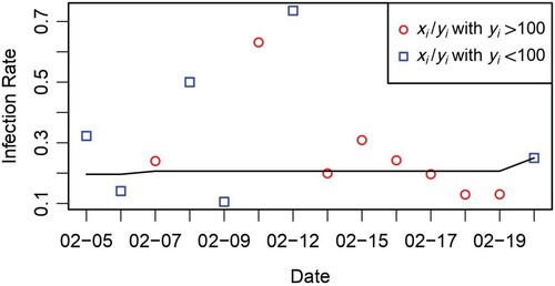
If there is no selection bias, it is a standard current status data problem discussed extensively in the statistical literature, for example, (Sun, 2006). The nonparametric likelihood method can be used directly to estimate $G_i$. The observed likelihood function is (1) $\prod _{i=1}^{14}\frac{y_i!}{x_i!(y_i-x_i)!}{\left(G_i\right)}^{x_i}{(1-G_i)}^{y_i-x_i}.$(1) However, Figure 1 shows that the observed frequency and estimated probability on each day have a large discrepancy, especially in the first week. This demonstrates that the random selection process was violated.

Figure 1. Comparison of the observed detection rates $\{x_i/y_i{\}}_{i=1}^{14}$ and estimated ones if the selection bias is ignored. $x_i$ represents number of patients that were tested positive at day i, and $y_i$ is the total number of tests at day i. Scatter points are the rate of $x_i/y_i$, where red and blue colours differentiate whether $y_i>100$ or not. Black line shows the estimated detection rates $\{G_i{\}}_{i=1}^{14}$.

Next, we provide a novel mixture modelling strategy that fully utilizes the non-random sampling. Before the quarantine, people were unaware of the existence of virus on the Diamond Princess cruise ship. The cruise had shows and dance parties and opened public facilities that attracted large crowds, including fitness clubs, theatres, casinos, bars and buffet-style restaurants. During this period, all passengers and crew members were susceptible to the COVID-19. After the quarantine, people gradually realized the high contagiosity of the virus and began to take actions to avoid the infection. The anti-epidemic measures became stricter as time went on. Passengers with confirmed cases were reported to be taken ashore for treatment. Some individuals even left the cruise in advance. Therefore, it is reasonable to assume some individuals were insusceptible at this stage. Taking the above facts and the incubation period into account, we suppose the detection patterns of the first week and second week of the quarantine period are different. We divide subjects into susceptible and insusceptible individuals and suppose the two weeks have different compositions. All the people in the first week are susceptible, and the proportion of insusceptible individuals in the second week grows.

We assume a cure mixture model (Farewell, 1982) for the detection time ${\xi }_{ij}$. Specifically, the mixture modelling of the cure rate assumes a decomposition of the detection time, (2) ${\xi }_{ij}={\eta }_{ij}{\xi }_{ij}^{\ast }+(1-{\eta }_{ij})\mathrm{\infty },j=1,\dots ,y_i,i=1,\dots ,14,$(2) where ${\xi }_{ij}^{\ast }<\mathrm{\infty }$ denotes the detection time of a susceptible subject, and ${\eta }_{ij}$ indicates, by the value 1 or 0, whether the sampled subject is susceptible or not.

It is worthy notifying that the observed data of most infectious diseases, including COVID-19 on the Diamond Prince cruise ship, are aggregated data. The individual data are unavailable. Therefore, models on specific subjects are impossible to be identified. We have the aggregated data on each testing day. The detection results of each day should follow different patterns, because the anti-epidemic measures became stricter and the insusceptible proportions increased as time went on. Thus, we assume the susceptible proportion and the distribution function of detection time depend only on testing day i. Let $Pr({\eta }_{ij}=1)={\lambda }_i$, the proportion of susceptible patients among tested subjects at day i. At each day i, we suppose that tested individuals are a mixture of a proportion of ${\lambda }_i$ susceptible individuals who eventually get infected and a proportion of $1-{\lambda }_i$ who are not susceptible to COVID-19 and will never get infected. Let $F\left(x\right)$ be the distribution function of detection time of a susceptible subject, that is, ${\xi }_{ij}^{\ast }\sim F\left(x\right)$. Model (2(2) ${\xi }_{ij}={\eta }_{ij}{\xi }_{ij}^{\ast }+(1-{\eta }_{ij})\mathrm{\infty },j=1,\dots ,y_i,i=1,\dots ,14,$(2) ) is equivalent to ${\xi }_{ij}\sim {\lambda }_{i}F\left(x\right)+(1-{\lambda }_i)I(x=\mathrm{\infty }),j=1,\dots ,y_i,i=1,\dots ,14.$For notation simplicity, we write $F_i\doteq F\left(i\right)$. $F_i$ is the probability that a susceptible infected individual can be detected by PCR test on day i. The proposed model is useful since a proportion of tested subjects will never be infected by COVID-19. This model is like survival models with cure rate, which have arisen in many disciplines (e.g. biomedical sciences, economics, sociology, engineering science, etc) and have received much attention (Lu & Ying, 2004; Wang et al., 2020).

Motivated by the priority in choosing symptomatic or high-risk groups, all chosen people in the first week were likely to be infected and detected, and the susceptible probabilities maintained a high level nearly 1. Since symptomatic and vulnerable individuals were tested first and some sick individuals disembarked at the end of first week, it is expected that the proportions of non-susceptible individuals became larger as time went by. In other words, starting from the second week, ${\lambda }_i,i=8,9,\dots ,14$, decrease. We suppose the mixture proportion ${\lambda }_i$ varies across i in the logistic form to add model flexibility. Specifically, we assume ${\lambda }_i=1,1⩽i⩽7$, and (3) ${\lambda }_i=\frac{\exp ({\theta }_1+{\theta }_2(i-7\left)\right)}{1+\exp ({\theta }_1+{\theta }_2(i-7\left)\right)},{\theta }_2<0,i=8,9,\dots ,14,$(3) with unknown parameters ${\theta }_1$ and ${\theta }_2$. It is easy to see that suspectable proportions in the first week are supposed to be the same, and the suspectable probabilities ${\lambda }_i,8⩽i⩽14$ in the second week have a logistic regression form and decrease as i increases. Different forms of ${\lambda }_i$ are designed to account for the data collection difference between the two weeks. Under the proposed model, the true detected number during the quarantine period, N, is $N=\left(\sum _{i=1}^7{y}_i\right)F_{14}+\left(\sum _{i=8}^{14}{\lambda }_i{y}_i\right)F_{14}+(n^{\ast }-n){\lambda }_{14}{F}_{14}.$In summary, we formulate a cure model by assuming that the underlying population on the Diamond Princess cruise ship is a mixture of susceptible and non-susceptible subjects. All susceptible subjects are vulnerable to be infected and detected by COVID-19, while the nonsusceptible ones are never infected and detected. Thus, we model separately the detection distribution for susceptible individuals and the fraction of nonsusceptible ones.

2.2. Estimation

The proposed mixture model uses a nonparametric approach to estimate the detection distribution F and a parametric approach to estimate the suspectable proportion λ. Since $Pr({\delta }_{ij}=1)={\lambda }_i{F}_i$, the conditional expectation of $x_i$ is $\mathbb{E}\left(x_i\right)=y_i{\lambda }_i{F}_i$. The observed data are summarized as $\left\{\right(x_i,y_i);i=1,\dots ,14\}$, which are constituted by $n=\sum _{i=1}^{14}{y}_i$ independent and identically distributed random replications. The observed likelihood is then written as $\begin{array}{rl}{L}_n(F,\theta )& =\prod _{i=1}^{14}\prod _{j=1}^{y_i}{\left({\lambda }_i{F}_i\right)}^{{\delta }_{ij}}{(1-{\lambda }_i{F}_i)}^{1-{\delta }_{ij}}\\ & =\prod _{i=1}^{14}{\left({\lambda }_i{F}_i\right)}^{\sum _{j=1}^{y_i}{\delta }_{ij}}{(1-{\lambda }_i{F}_i)}^{\sum _{j=1}^{y_i}(1-{\delta }_{ij})}\\ & =\prod _{i=1}^{14}{\left({\lambda }_i{F}_i\right)}^{x_i}{(1-{\lambda }_i{F}_i)}^{y_i-x_i}.\end{array}$Suppose ${\lambda }_i>0,F_i>0$. The log-likelihood is $\begin{array}{rl}{\ell }_n(F,\theta )& =\sum _{i=1}^{14}\sum _{j=1}^{y_i}\{{\delta }_{ij}\log ({\lambda }_i{F}_i)+(1-{\delta }_{ij})\log (1-{\lambda }_i{F}_i\left)\right\}\\ & =\sum _{i=1}^{14}\{x_i\log ({\lambda }_i{F}_i)+(y_i-x_i)\log (1-{\lambda }_i{F}_i\left)\right\}.\end{array}$We view F as a piecewise constant non-decreasing nonparametric function that only jumps at $i=1,\dots ,14$. So far we have 16 unknown parameters $F_i,i=1,\dots ,14,{\theta }_1$ and ${\theta }_2$ but only have 14 pairs of observed data. To ensure identifiability, we impose the constraints $F_2=(F_1+F_3)/2$ and $F_{13}=F_{12}$. Then $\begin{array}{rl}{\ell }_n(F,\theta )& =\sum _{i=1,i\ne 2}^7\{x_i\log F_i+(y_i-x_i)\log (1-F_i\left)\right\}\\ & +\{x_2\log ((F_1+F_3)/2)+(y_2-x_2)\log (1-(F_1+F_3)/2\left)\right\}\\ & +\sum _{i=8,i\ne 13}^{14}\{x_i\log ({\lambda }_i{F}_i)+(y_i-x_i)\log (1-{\lambda }_i{F}_i\left)\right\}\\ & +x_{13}\log \left({\lambda }_{13}{F}_{12}\right)+(y_{13}-x_{13})\log (1-{\lambda }_{13}{F}_{12}).\end{array}$The maximum likelihood estimators (MLEs) $({\hat{F}}_i,{\hat{\theta }}_k)$ are derived by maximizing ${\ell }_n(F,\theta )$, that is, $({\hat{F}}_i,{\hat{\theta }}_k)={\text{argmax}}_{F,\theta }{\ell }_n(F,\theta ),1⩽i⩽14,i\ne 2,13,k=1,2.$Then, we can estimate N by $\hat{N}=\left(\sum _{i=1}^7{y}_i\right){\hat{F}}_{14}+\left(\sum _{i=8}^{14}{\hat{\lambda }}_i{y}_i\right){\hat{F}}_{14}+(n^{\ast }-n){\hat{\lambda }}_{14}{\hat{F}}_{14},$where ${\hat{\lambda }}_i=\exp ({\hat{\theta }}_1+{\hat{\theta }}_2(i-7\left)\right)/\{1+\exp ({\hat{\theta }}_1+{\hat{\theta }}_2(i-7)\left)\right\}$ for $i=8,\dots ,14$.

Remark 2.1

We only have 14 days aggregated data, but 28 unknown parameters, ${\lambda }_i$, $F_i$, $i=1,\dots ,14$. To overcome the non-identifiability, we carefully account for the data characteristics, estimate $F_i$ nonparametrically with two constraints, and impose a parametric model on ${\lambda }_i$. Logistic regression is the most common model for the proportion. The logistic model provides an approximation for the susceptible proportion. We set one regression coefficient as negative to describe the decreasing trend. One may also use other parametric models, for example, the probit model. We have fitted the probit model ${\lambda }_i=\mathrm{\Phi }({\theta }_5+{\theta }_{6}i),8⩽i⩽14,{\theta }_6<0$ to the Diamond Princess cruise ship data and found the estimated number of cumulative infection cases was 1072, which is almost the same with the estimated number 1074 using the logistic model. This shows the robustness and rationality of the imposed assumptions. If we impose strict assumptions on $F_i$ and constraints on some ${\lambda }_i$, one may also estimate ${\lambda }_i$ nonparametrically.

Remark 2.2

The two constraints $F_2=(F_1+F_3)/2$ and $F_{13}=F_{12}$ are imposed according to the preliminary data analysis. We can impose other alternative constraints. For example, we assume a Weibull distribution for F which is commonly used in epidemical modelling. Suppose $F_i=F\left(i\right)=1-\exp \{-({\theta }_{4}i{)}^{{\theta }_3}\},i=1,2,\dots ,14.$ Maximum likelihood is used for parameter estimation. Applying this parametric approach to the Diamond Princess cruise data, the estimated total infected number at the end of quarantine is 1036, which is quite close to the estimated number using the proposed nonparametric method. This shows the robustness and rationality of the imposed constraints.

3. Asymptotic results

In this section, we give the large sample properties of the proposed estimators. Write $\begin{array}{rl}\ell (F,\theta )& \doteq \underset{n\to \mathrm{\infty }}{lim}{n}^{-1}{\ell }_n(F,\theta )\\ & =\sum _{i=1}^{14}{p}_i\{{\lambda }_i{F}_i\log ({\lambda }_i{F}_i)+(1-{\lambda }_i{F}_i)\log (1-{\lambda }_i{F}_i\left)\right\}\\ & =\sum _{i=1,i\ne 2}^7{p}_i\{F_i\log F_i+(1-F_i)\log (1-F_i\left)\right\}\\ & +p_2\{\frac{F_1+F_3}{2}\log \frac{F_1+F_3}{2}+\frac{2-(F_1+F_3)}{2}\log \frac{2-(F_1+F_3)}{2}\}\\ & +\sum _{i=8,i\ne 13}^{14}{p}_i\{{\lambda }_i{F}_i\log \left({\lambda }_i{F}_i\right)+(1-{\lambda }_i{F}_i)\log (1-{\lambda }_i{F}_i)\}\\ & +p_{13}\{{\lambda }_{13}{F}_{12}\log \left({\lambda }_{13}{F}_{12}\right)+(1-{\lambda }_{13}{F}_{12})\log (1-{\lambda }_{13}{F}_{12})\},\end{array}$where $p_i=\underset{n\to \mathrm{\infty }}{lim}{y}_i/n$.

For notation simplicity, let $\widehat{\text{β}}=({\widehat{\text{β}}}_1,\dots ,{\widehat{\text{β}}}_{14}{)}^{\mathrm{\top }}=({\hat{F}}_1,{\hat{F}}_3,\dots ,{\hat{F}}_{12},{\hat{F}}_{14},{\hat{\theta }}_1,{\hat{\theta }}_2{)}^{\mathrm{\top }}$. Denote the true value of $\text{β}$ as ${\text{β}}_0=(F_{1,0},F_{3,0},\dots ,F_{12,0},F_{14,0},{\theta }_{1,0},{\theta }_{2,0}{)}^{\mathrm{\top }}$, and denote $\ell (F,\theta )$ as $\ell \left(\text{β}\right)$. The likelihood function $\ell \left(\text{β}\right)$ is differentiable with respect to each component of $\text{β}$. Define $\mathit{V}\left(\text{β}\right)=-{\mathrm{d}}^2\ell \left(\text{β}\right)/\mathrm{d}{\text{β}}^2$, ${\mathbb{R}}_{-}=(-\mathrm{\infty },0)$, where the specific form of $\mathit{V}\left(\text{β}\right)$ is given in the Appendix.

We impose the following regularity conditions.

(C1)	The parameter space $\mathcal{B}$ is a bounded and closed subset of $(0,1{)}^{12}\times \mathbb{R}\times {\mathbb{R}}_{-}$.
(C2)	$\mathit{V}\left({\text{β}}_0\right)$ is a non-singular $14\times 14$ matrix.
(C3)	${\text{β}}_0$ is the unique solution to ${\ell }^{\prime }\left(\text{β}\right)=0$ for $\text{β}\in \mathcal{B}$, where ${\ell }^{\prime }\left(\text{β}\right)=\mathrm{d}\ell \left(\text{β}\right)/\mathrm{d}\text{β}$.

Theorem 3.1

Under the regularity conditions (C1)–(C3), $\widehat{\text{β}}$ converges to ${\text{β}}_0$ almost surely.

Theorem 3.2

Under the regularity conditions (C1)–(C3), $n^{1/2}\{\widehat{\text{β}}-{\text{β}}_0\}$ converges asymptotically to a normal distribution $N(0,\mathit{V}({\text{β}}_0{)}^{-1})$.

Based on the theoretical results for $\widehat{\text{β}}$ established in Theorems 3.1 and 3.2, we can follow the delta method to easily get the asymptotic properties of ${\hat{F}}_2$ and ${\hat{F}}_{13}$.

4. Simulation studies

In this section, we conduct simulation studies to assess the finite sample performance of the proposed method. We generate data to mimic the PCR testing data on Diamond Princess cruise ship. Specifically, suppose the total number of people (include passengers and crew members) on the cruise for quarantine is $n^{\ast }=3711$. There are 14 pairs of observations $\left\{\right(x_i,y_i){\}}_{i=1}^{14}$, where $(y_1,\dots ,y_{14}{)}^{\mathrm{\top }}=(31,71,171,6,57,103,53,221,217,289,504,681,607,52{)}^{\mathrm{\top }}$ is consisted by the number of total tests each day. The susceptible probabilities $\begin{array}{rl}& {\lambda }_i=1,1⩽i⩽7,\\ & {\lambda }_i=\frac{\exp ({\theta }_1+{\theta }_2(i-7\left)\right)}{1+\exp ({\theta }_1+{\theta }_2(i-7\left)\right)},8⩽i⩽14,\end{array}$with ${\theta }_1=-0.518$, ${\theta }_2=-0.232$. Given $y_i$, $x_i$ is generated from Binomial distribution B$(y_i,{\lambda }_i{F}_i)$ with success probability ${\lambda }_i{F}_i$, where $F_i,1⩽i⩽14$ are set as $F=(F_1,\dots ,F_{14}{)}^{\mathrm{\top }}$=(0.208, 0.208, 0.208, 0.208, 0.208, 0.631, 0.696, 0.696, 0.850, 0.900, 0.950, 0.950, 1.000, 1.000)${}^{\mathrm{\top }}$.

Under this configuration, the true number of infections is N = 1042. We simulate 500 datasets and use bootstrap to derive estimated standard errors and confidence intervals of the unknown parameters. 100 bootstrap samples are generated based on the nonparametric mixture model with estimated parameters. The 95% confidence intervals (CI) are derived through normal approximation, where the estimated standard errors are calculated as the standard deviation of bootstrap sample estimators.

Table 2. Simulation results.

Parameter	True	Bias	SD	SE	CP
$F_1$	0.208	$-0.023$	0.036	0.039	95.6
$F_2$	0.208	$-0.012$	0.025	0.025	92.6
$F_3$	0.208	0.001	0.025	0.025	95.6
$F_4$	0.208	0.011	0.034	0.039	98.8
$F_5$	0.208	0.024	0.040	0.043	95.4
$F_6$	0.631	$-0.005$	0.044	0.044	95.4
$F_7$	0.696	$-0.001$	0.053	0.052	93.4
$F_8$	0.696	0.018	0.070	0.064	92.4
$F_9$	0.850	$-0.024$	0.104	0.093	91.0
$F_{10}$	0.900	$-0.019$	0.096	0.093	94.8
$F_{11}$	0.950	$-0.025$	0.089	0.085	94.6
$F_{12}$	0.950	0.002	0.085	0.074	97.2
$F_{13}$	1.000	$-0.048$	0.085	0.074	92.2
$F_{14}$	1.000	$-0.002$	0.011	0.011	95.8
N	1043	13.55	59.62	53.59	96.6
${\theta }_1$	$-0.518$	$-0.007$	0.216	0.225	96.2
${\theta }_2$	$-0.232$	0.008	0.045	0.046	95.6
${\lambda }_8$	0.321	0.001	0.039	0.041	95.8
${\lambda }_9$	0.272	0.003	0.030	0.031	96.2
${\lambda }_{10}$	0.229	0.004	0.024	0.023	96.4
${\lambda }_{11}$	0.191	0.005	0.020	0.018	95.8
${\lambda }_{12}$	0.157	0.005	0.019	0.017	96.0
${\lambda }_{13}$	0.129	0.006	0.019	0.017	95.8
${\lambda }_{14}$	0.105	0.006	0.019	0.018	95.4

Table 1 summarizes the simulation results, where the true parameters, the empirical biases (Bias), the empirical standard deviations (SD), the estimated standard errors (SE) and the empirical coverage probabilities (CP) are given. We can conclude that the empirical biases are negligible, the empirical standard deviations and estimated standard errors match each other quite well, and the empirical coverage probabilities are close to the nominal one 95%.

5. Real data analysis

In this Section, we apply the proposed method to the Diamond Princess cruise data to show its practical utility. We use the time series daily report PCR testing data, including the number of tests and number of patients testing positive each day during the quarantine period, to estimate the distribution of detection time, and the varying proportions of susceptible individuals, along with the total number of infections that can be detected. The data are publicly available, for example, in Table 1 of Mizumoto et al. (2020).

In the real data, 14 pairs of $(x_i,y_i)$ are observed. As stated in Section 2, we impose the constraints $F_2=(F_1+F_3)/2$ and $F_{13}=F_{12}$ to solve the potential identifiability problem. Under the proposed nonparametric mixture modelling framework, the maximum likelihood estimators (MLEs) are derived by maximizing the joint log-likelihood with time series daily report data. The nlm() function in R is employed to estimate $F_i,1⩽i⩽14,i\ne 2,13$, ${\theta }_1$, and ${\theta }_2$. Let ${\hat{F}}_2=({\hat{F}}_1+{\hat{F}}_3)/2$ and ${\hat{F}}_{13}={\hat{F}}_{12}$. The proportion of susceptible individuals incorporated in the PCR test at day i, ${\hat{\lambda }}_i$, can be derived from the logistic regression form with estimated ${\hat{\theta }}_1$ and ${\hat{\theta }}_2$. We use the estimated parameters to simulate bootstrap samples, which include time series daily data of number of tests and confirmed cases. 200 bootstrap samples are generated to estimate the standard errors, and the confidence intervals are based on normal approximation. Table 3 lists the estimators ${\hat{F}}_i,1⩽i⩽14$, ${\hat{\theta }}_i,i=1,2$, $\hat{N}$, ${\hat{\lambda }}_i,8⩽i⩽14$, the corresponding estimated standard errors and confidence intervals. The estimated $F_1$ is about 0.2 and $F_9$ is close to 1 (Table 3), which means that about 20% of susceptible individuals will be detected at the beginning of quarantine. And 9 days later, all the susceptible individuals on the board will be detected.

Table 3. MLEs and the corresponding confidence intervals in real data analysis.

Parameter	Estimate	Standard Error	Confidence Interval
$F_1$	0.208	0.037	(0.136, 0.281)
$F_2$	0.208	0.024	(0.162, 0.255)
$F_3$	0.208	0.024	(0.162, 0.255)
$F_4$	0.208	0.032	(0.145, 0.271)
$F_5$	0.208	0.035	(0.140, 0.276)
$F_6$	0.631	0.045	(0.543, 0.719)
$F_7$	0.696	0.052	(0.587, 0.790)
$F_8$	0.696	0.052	(0.587, 0.790)
$F_9$	1.000	0.090	(0.783, 1.000)
$F_{10}$	1.000	0.079	(0.803, 1.000)
$F_{11}$	1.000	0.063	(0.837, 1.000)
$F_{12}$	1.000	0.053	(0.855, 1.000)
$F_{13}$	1.000	0.053	(0.855, 1.000)
$F_{14}$	1.000	0.010	(0.981, 1.000)
N	1064	40.91	(984, 1144)
${\theta }_1$	−0.476	0.198	(−0.864, −0.089)
${\theta }_2$	−0.231	0.042	(−0.313, −0.149)
${\lambda }_8$	0.330	0.036	(0.259, 0.402)
${\lambda }_9$	0.281	0.027	(0.229, 0.333)
${\lambda }_{10}$	0.237	0.019	(0.200, 0.274)
${\lambda }_{11}$	0.198	0.014	(0.170, 0.226)
${\lambda }_{12}$	0.164	0.013	(0.138, 0.189)
${\lambda }_{13}$	0.134	0.014	(0.107, 0.161)
${\lambda }_{14}$	0.110	0.014	(0.081, 0.138)

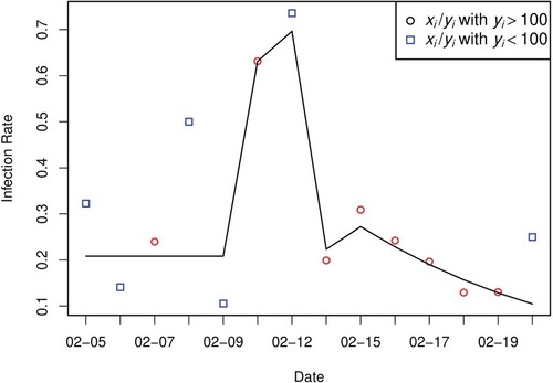
Figure 2 presents the observed detection rates $x_i/y_i$ (scatter points), along with the fitted detection rates ${\lambda }_i{F}_i$ (black solid line). We use different colours and different symbols to demonstrate $x_i/y_i$ with $y_i>100$ or $y_i<100$, respectively. For example, red circles represent scatter points $x_i/y_i$ with $y_i>100$, while blue squares describe scatter points $x_i/y_i$ with $y_i<100$. Figure 2 suggests that the estimated nonparametric distribution $F_i$ and the parametric susceptible proportion ${\lambda }_i$ characterize the pattern of detection quite well. This shows the plausibility of the assumption that ${\lambda }_i$ decreases with i in the logistic regression form.

In contrast to the officially reported 634 individuals with PCR-positive results after the 14 days quarantine, which as of April 27, 2020 had increased to 712 as released by the Johns Hopkins University, we conclude that the estimated total number should be 1064. Zhang et al. (2020) used a completely different method to estimate the reproductive number (R0) of the novel virus in the early stage of the outbreak and estimate the cumulative cases on the ship. They estimated the cumulative cases as 1514 (1384–1656) if the R0 value remained 2.28 as the early stage on the ship. If R0 value was reduced by 25% and 50%, the estimated total number of cumulative cases would be reduced to 1081 (981–1177) and 758 (697–817), respectively. A great deal of the transmission on the ship had occurred before the quarantine when people were even not notified about the virus. As the containment measures became stricter, it is expected that the R0 value reduced. We estimated the total number as 1064 (984–1144), which is almost in accordance with the number when the R0 value was reduced by 25%.

Figure 2. Comparison of the observed detection rates $\{x_i/y_i{\}}_{i=1}^{14}$ and fitted ones based on the proposed nonparametric mixture model. $x_i$ represents number of patients that were tested positive at day i, and $y_i$ is the total number of tests at day i. Scatter points are the rates of $x_i/y_i$, where red and blue colours differentiate whether $y_i>100$ or not. Black line shows the fitted detection rates $\{{\lambda }_i{F}_i{\}}_{i=1}^{14}$.

6. Concluding remarks

In this paper, motivated by the real PCR testing data on the Diamond Princess cruise ship, we propose a novel mixture model to estimate the distribution of detection time among susceptible subjects and the susceptible proportion among tested people each day. As a by-product, the total number that can be detected after the quarantine period is estimated as 1064, which means that 42.5% of infected cases were undetected on the cruise. The estimated number 1064 is larger than the released 712. The discrepancy might be caused by the false-negative result of the PCR test (Kucirka et al., 2020) or the occurrence of infection after the test. Some asymptomatic cases may be missed due to the imperfect sensitivity of the PCR test, and they had the high transmissibility. We conclude that COVID-19 spread in the cruise ship is easier and faster than in open spaces. Strict containment efforts should be scaled up prior to local outbreak.

Like all medical papers, we have to acknowledge the possible weakness in our approach. The COVID-19 data collected on the Diamond Princess cruise were very limited. All information was summarized in Table 1. We assume that each selected individual was tested by PCR only once and assume that the sensitivity of the test was 100%. This might be not true because small proportion of individuals may be tested twice or more, and there may be false positives. Our method should be modified if additional relevant testing information was available. Nevertheless, we believe our approach has at least reduced the possible bias in the data collection process, though our solution may not be a perfect one. We would be happy to read other innovative approaches from other authors in the future. During the outbreak of a pandemic, it would be useful to make quick statistical inference based on very limited information, though, it may not be a very accurate one. Besides, in the second week of the quarantine, the number of symptomatic and asymptomatic patients testing positive was publicly available. However, we did not take these information into consideration. Incorporating such data in statistical modelling warrants future research.

Acknowledgments

The authors thank the Editor, Professor Jun Shao, an Associate Editor and three reviewers for their insightful comments and suggestions that greatly improved the article.

Disclosure statement

No potential conflict of interest was reported by the authors.

Additional information

Funding

This work is partly supported by the National Natural Science Foundation of China [grant numbers 71931004, 11901200, 71971083, and 11971170] and the National Key R&D Program of China [grant numbers 2021YFA1000100, 2021YFA1000101].

Appendix

Proof of Theorem 3.1.

Proof of Theorem 3.1.

Write $\begin{array}{rl}\frac{1}{n}{\ell }_n^{\prime }\left(\text{β}\right)& =\frac{1}{n}\frac{\mathrm{d}{\ell }_n\left(\text{β}\right)}{\mathrm{d}\text{β}}=\frac{1}{n}\sum _{i=1}^{14}\sum _{j=1}^{y_i}\{{\delta }_{ij}\frac{\mathrm{d}\log \left({\lambda }_i{F}_i\right)}{\mathrm{d}\text{β}}+(1-{\delta }_{ij}\left)\frac{\mathrm{d}\log (1-{\lambda }_i{F}_i)}{\mathrm{d}\text{β}}\right\}\\ & \doteq \frac{1}{n}\sum _{i=1}^{14}\sum _{j=1}^{y_i}{\mathit{\zeta }}_{ij}\left(\text{β}\right),\end{array}$where $n=\sum _{i=1}^{14}{y}_i$, ${\mathit{\zeta }}_{ij}\left(\text{β}\right)=\left({\zeta }_{ij}^{\left(1\right)}\right(\text{β}),\dots ,{\zeta }_{ij}^{\left(14\right)}(\text{β}){)}^{\mathrm{\top }}\doteq ({\delta }_{ij}\mathrm{\partial }\log \left({\lambda }_i{F}_i\right)/\mathrm{\partial }{\text{β}}_1+(1-{\delta }_{ij})\mathrm{\partial }\log (1-{\lambda }_i{F}_i)/\mathrm{\partial }{\text{β}}_1,\dots ,{\delta }_{ij}\mathrm{\partial }\log \left({\lambda }_i{F}_i\right)/\mathrm{\partial }{\text{β}}_{14}+(1-{\delta }_{ij})\mathrm{\partial }\log (1-{\lambda }_i{F}_i)/\mathrm{\partial }{\text{β}}_{14}{)}^{\mathrm{\top }}$ is a 14-dimensional vector with $\begin{array}{rl}{\zeta }_{ij}^{\left(1\right)}\left(\text{β}\right)& =I(i=1)(\frac{{\delta }_{ij}}{F_1}-\frac{1-{\delta }_{ij}}{1-F_1})+I(i=2)(\frac{{\delta }_{ij}}{F_1+F_3}-\frac{1-{\delta }_{ij}}{2-F_1-F_3}),\\ {\zeta }_{ij}^{\left(2\right)}\left(\text{β}\right)& =I(i=3)(\frac{{\delta }_{ij}}{F_3}-\frac{1-{\delta }_{ij}}{1-F_3})+I(i=2)(\frac{{\delta }_{ij}}{F_1+F_3}-\frac{1-{\delta }_{ij}}{2-F_1-F_3}),\\ {\zeta }_{ij}^{\left(3\right)}\left(\text{β}\right)& =I(i=4)(\frac{{\delta }_{ij}}{F_4}-\frac{1-{\delta }_{ij}}{1-F_4}),\\ {\zeta }_{ij}^{\left(4\right)}\left(\text{β}\right)& =I(i=5)(\frac{{\delta }_{ij}}{F_5}-\frac{1-{\delta }_{ij}}{1-F_5}),\\ {\zeta }_{ij}^{\left(5\right)}\left(\text{β}\right)& =I(i=6)(\frac{{\delta }_{ij}}{F_6}-\frac{1-{\delta }_{ij}}{1-F_6}),\\ {\zeta }_{ij}^{\left(6\right)}\left(\text{β}\right)& =I(i=7)(\frac{{\delta }_{ij}}{F_7}-\frac{1-{\delta }_{ij}}{1-F_7}),\\ {\zeta }_{ij}^{\left(7\right)}\left(\text{β}\right)& =I(i=8)(\frac{{\delta }_{ij}}{F_8}-\frac{(1-{\delta }_{ij}){\lambda }_i}{1-{\lambda }_i{F}_8}),\end{array}$ $\begin{array}{rl}{\zeta }_{ij}^{\left(8\right)}\left(\text{β}\right)& =I(i=9)(\frac{{\delta }_{ij}}{F_9}-\frac{(1-{\delta }_{ij}){\lambda }_i}{1-{\lambda }_i{F}_9}),\\ {\zeta }_{ij}^{\left(9\right)}\left(\text{β}\right)& =I(i=10)(\frac{{\delta }_{ij}}{F_{10}}-\frac{(1-{\delta }_{ij}){\lambda }_i}{1-{\lambda }_i{F}_{10}}),\\ {\zeta }_{ij}^{\left(10\right)}\left(\text{β}\right)& =I(i=11)(\frac{{\delta }_{ij}}{F_{11}}-\frac{(1-{\delta }_{ij}){\lambda }_i}{1-{\lambda }_i{F}_{11}}),\\ {\zeta }_{ij}^{\left(11\right)}\left(\text{β}\right)& =I(i=12)(\frac{{\delta }_{ij}}{F_{12}}-\frac{(1-{\delta }_{ij}){\lambda }_i}{1-{\lambda }_i{F}_{12}})+I(i=13)(\frac{{\delta }_{ij}}{F_{12}}-\frac{(1-{\delta }_{ij}){\lambda }_i}{1-{\lambda }_i{F}_{12}}),\\ {\zeta }_{ij}^{\left(12\right)}\left(\text{β}\right)& =I(i=14)(\frac{{\delta }_{ij}}{F_{14}}-\frac{(1-{\delta }_{ij}){\lambda }_i}{1-{\lambda }_i{F}_{14}}),\\ {\zeta }_{ij}^{\left(13\right)}\left(\text{β}\right)& =I(i=8,\dots ,14;i\ne 13)\{{\delta }_{ij}(1-{\lambda }_i)-\frac{(1-{\delta }_{ij}){\lambda }_i{F}_i(1-{\lambda }_i)}{1-{\lambda }_i{F}_i}\}\\ & +I(i=13)\{{\delta }_{ij}(1-{\lambda }_i)-\frac{(1-{\delta }_{ij}){\lambda }_i{F}_{12}(1-{\lambda }_i)}{1-{\lambda }_i{F}_{12}}\},\\ {\zeta }_{ij}^{\left(14\right)}\left(\text{β}\right)& =I(i=8,\dots ,14;i\ne 13)\{{\delta }_{ij}(1-{\lambda }_i)(i-7)-\frac{(1-{\delta }_{ij}){\lambda }_i{F}_i(1-{\lambda }_i)(i-7)}{1-{\lambda }_i{F}_i}\}\\ & +I(i=13)\{{\delta }_{ij}(1-{\lambda }_i)(i-7)-\frac{(1-{\delta }_{ij}){\lambda }_i(1-{\lambda }_i)(i-7)F_{12}}{1-{\lambda }_i{F}_{12}}\},\end{array}$where the last two equalities hold since $\mathrm{\partial }{\lambda }_i/\mathrm{\partial }{\theta }_1={\lambda }_i(1-{\lambda }_i)$ and $\mathrm{\partial }{\lambda }_i/\mathrm{\partial }{\theta }_2={\lambda }_i(1-{\lambda }_i)(i-7)$ for $i=8,9,\dots ,14$.

It is easy to show that ${\ell }^{\prime }\left({\text{β}}_0\right)=\mathbf{0}$, where ${\ell }^{\prime }\left(\text{β}\right)=\underset{n\to \mathrm{\infty }}{lim}{n}^{-1}{\ell }_n^{\prime }\left(\text{β}\right)$. According to the regularity condition (C1), $\left\{{\mathit{\zeta }}_{ij}\right(\text{β});\text{β}\in \mathcal{B}\}$ is a Glivenko–Cantelli class (van der Vaart & Wellner, 1996). It follows from the Glivenko–Cantelli theorem (van der Vaart & Wellner, 1996) that (A1) $\underset{\text{β}\in \mathcal{B}}{sup}\Vert n^{-1}{\ell }_n^{\prime }\left(\text{β}\right)-{\ell }^{\prime }\left(\text{β}\right)\Vert \to 0$(A1) almost surely. Note that $\widehat{\text{β}}$ is the maximizer of $n^{-1}{\ell }_n\left(\text{β}\right)$, and $n^{-1}{\ell }_n\left(\text{β}\right)$ is differentiable in terms of $\text{β}$. Hence $n^{-1}{\ell }_n^{\prime }\left(\widehat{\text{β}}\right)=0$. This, combined with (A1(A1) $\underset{\text{β}\in \mathcal{B}}{sup}\Vert n^{-1}{\ell }_n^{\prime }\left(\text{β}\right)-{\ell }^{\prime }\left(\text{β}\right)\Vert \to 0$(A1) ), implies that ${\ell }^{\prime }\left(\widehat{\text{β}}\right)=o_p\left(1\right)$. Then, according to the regularity condition (C3), $\widehat{\text{β}}$ converges to ${\text{β}}_0$ almost surely.

Proof of Theorem 3.1.

Proof of Theorem 3.2.

Expanding the first derivative of $n^{-1/2}{\ell }_n^{\prime }\left(\text{β}\right)$ around the true value ${\text{β}}_0$, we get (A2) $\begin{array}{rl}\mathbf{0}=n^{-1/2}{\ell }_n^{\prime }\left(\widehat{\text{β}}\right)& =n^{-1/2}{\ell }_n^{\prime }\left({\text{β}}_0\right)+n^{-1}{\ell }_n^{″}\left(\widetilde{\text{β}}\right)n^{1/2}(\widehat{\text{β}}-{\text{β}}_0)\\ & =n^{-1/2}{\ell }_n^{\prime }\left({\text{β}}_0\right)+n^{-1}{\ell }_n^{″}\left({\text{β}}_0\right)n^{1/2}(\widehat{\text{β}}-{\text{β}}_0)+o_p\left(1\right),\end{array}$(A2) where $\widetilde{\text{β}}$ lies between $\widehat{\text{β}}$ and ${\text{β}}_0$, and the last equality follows from the continuity of ${\ell }_n^{\prime }\left(\text{β}\right)$. Note that $n^{-1}E\left(x_i\right)\to p_i{\lambda }_i{F}_i$ as $n\to \mathrm{\infty }$, where $p_i=\underset{n\to \mathrm{\infty }}{lim}{y}_i/n$, $i=1,\dots ,14$. According to the regularity condition (C1) and the law of large numbers, $-n^{-1}{\ell }_n^{″}\left({\text{β}}_0\right)\to \mathit{V}\left({\text{β}}_0\right)$, where each element of the matrix $\mathit{V}\left(\text{β}\right)=\left(v_{ij}\right(\text{β}){)}_{1⩽i,j⩽14}$ is given as follows: $\begin{array}{rl}{v}_{11}\left(\text{β}\right)& =-\underset{n\to \mathrm{\infty }}{lim}\frac{1}{n}\frac{{\mathrm{\partial }}^2{\ell }_n(F,\theta )}{\mathrm{\partial }{F}_1^2}=\frac{p_1}{F_1}+\frac{p_1}{(1-F_1)}+\frac{p_2}{2(F_1+F_3)}+\frac{p_2}{2(2-F_1-F_3)},\\ v_{12}\left(\text{β}\right)& =-\underset{n\to \mathrm{\infty }}{lim}\frac{1}{n}\frac{{\mathrm{\partial }}^2{\ell }_n(F,\theta )}{\mathrm{\partial }{F}_1\mathrm{\partial }{F}_3}=\frac{p_2}{2(F_1+F_3)}+\frac{p_2}{2(2-F_1-F_3)},\\ v_{1j}\left(\text{β}\right)& =0,j=3,\dots ,14,\\ v_{21}\left(\text{β}\right)& =v_{12}\left(\text{β}\right),\\ v_{22}\left(\text{β}\right)& =-\underset{n\to \mathrm{\infty }}{lim}\frac{1}{n}\frac{{\mathrm{\partial }}^2{\ell }_n(F,\theta )}{\mathrm{\partial }{F}_3^2}=\frac{p_3}{F_3}+\frac{p_3}{(1-F_3)}+\frac{p_2}{2(F_1+F_3)}+\frac{p_2}{2(2-F_1-F_3)},\\ v_{2j}\left(\text{β}\right)& =0,j=3,\dots ,14,\\ v_{33}\left(\text{β}\right)& =-\underset{n\to \mathrm{\infty }}{lim}\frac{1}{n}\frac{{\mathrm{\partial }}^2{\ell }_n(F,\theta )}{\mathrm{\partial }{F}_4^2}=\frac{p_4}{F_4}+\frac{p_4}{(1-F_4)},\\ v_{3j}\left(\text{β}\right)& =0,j=1,\dots ,14,j\ne 3,\\ v_{44}\left(\text{β}\right)& =-\underset{n\to \mathrm{\infty }}{lim}\frac{1}{n}\frac{{\mathrm{\partial }}^2{\ell }_n(F,\theta )}{\mathrm{\partial }{F}_5^2}=\frac{p_5}{F_5}+\frac{p_5}{(1-F_5)},\\ v_{4j}\left(\text{β}\right)& =0,j=1,\dots ,14,j\ne 4,\\ v_{55}\left(\text{β}\right)& =-\underset{n\to \mathrm{\infty }}{lim}\frac{1}{n}\frac{{\mathrm{\partial }}^2{\ell }_n(F,\theta )}{\mathrm{\partial }{F}_6^2}=\frac{p_6}{F_6}+\frac{p_6}{(1-F_6)},\\ v_{5j}\left(\text{β}\right)& =0,j=1,\dots ,14,j\ne 5,\\ v_{66}\left(\text{β}\right)& =-\underset{n\to \mathrm{\infty }}{lim}\frac{1}{n}\frac{{\mathrm{\partial }}^2{\ell }_n(F,\theta )}{\mathrm{\partial }{F}_7^2}=\frac{p_7}{F_7}+\frac{p_7}{(1-F_7)},\\ v_{6j}\left(\text{β}\right)& =0,j=1,\dots ,14,j\ne 6,\\ v_{7j}\left(\text{β}\right)& =0,j=1,\dots ,14,j\ne 7,13,14,\end{array}$ $\begin{array}{rl}{v}_{77}\left(\text{β}\right)& =-\underset{n\to \mathrm{\infty }}{lim}\frac{1}{n}\frac{{\mathrm{\partial }}^2{\ell }_n(F,\theta )}{\mathrm{\partial }{F}_8^2}=\frac{{\lambda }_8{p}_8}{F_8}+\frac{{\lambda }_8^2{p}_8}{(1-{\lambda }_8{F}_8)},\\ v_{7,13}\left(\text{β}\right)& =-\underset{n\to \mathrm{\infty }}{lim}\frac{1}{n}\frac{{\mathrm{\partial }}^2{\ell }_n(F,\theta )}{\mathrm{\partial }{F}_8\mathrm{\partial }{\theta }_1}=\frac{p_8{\lambda }_8(1-{\lambda }_8)}{1-{\lambda }_8{F}_8},\\ v_{7,14}\left(\text{β}\right)& =-\underset{n\to \mathrm{\infty }}{lim}\frac{1}{n}\frac{{\mathrm{\partial }}^2{\ell }_n(F,\theta )}{\mathrm{\partial }{F}_8\mathrm{\partial }{\theta }_2}=\frac{p_8{\lambda }_8(1-{\lambda }_8)}{1-{\lambda }_8{F}_8},\\ v_{8j}\left(\text{β}\right)& =0,j=1,\dots ,14,j\ne 8,13,14,\\ v_{8,8}\left(\text{β}\right)& =-\underset{n\to \mathrm{\infty }}{lim}\frac{1}{n}\frac{{\mathrm{\partial }}^2{\ell }_n(F,\theta )}{\mathrm{\partial }{F}_9^2}=\frac{{\lambda }_9{p}_9}{F_9}+\frac{{\lambda }_9^2{p}_9}{(1-{\lambda }_9{F}_9)},\\ v_{8,13}\left(\text{β}\right)& =-\underset{n\to \mathrm{\infty }}{lim}\frac{1}{n}\frac{{\mathrm{\partial }}^2{\ell }_n(F,\theta )}{\mathrm{\partial }{F}_9\mathrm{\partial }{\theta }_1}=\frac{p_9{\lambda }_9(1-{\lambda }_9)}{1-{\lambda }_9{F}_9},\\ v_{8,14}\left(\text{β}\right)& =-\underset{n\to \mathrm{\infty }}{lim}\frac{1}{n}\frac{{\mathrm{\partial }}^2{\ell }_n(F,\theta )}{\mathrm{\partial }{F}_9\mathrm{\partial }{\theta }_2}=\frac{2p_9{\lambda }_9(1-{\lambda }_9)}{1-{\lambda }_9{F}_9},\\ v_{9j}\left(\text{β}\right)& =0,j=1,\dots ,14,j\ne 9,13,14,\\ v_{9,9}\left(\text{β}\right)& =-\underset{n\to \mathrm{\infty }}{lim}\frac{1}{n}\frac{{\mathrm{\partial }}^2{\ell }_n(F,\theta )}{\mathrm{\partial }{F}_{10}^2}=\frac{{\lambda }_{10}{p}_{10}}{F_{10}}+\frac{{\lambda }_{10}^2{p}_{10}}{(1-{\lambda }_{10}{F}_{10})},\\ v_{9,13}\left(\text{β}\right)& =-\underset{n\to \mathrm{\infty }}{lim}\frac{1}{n}\frac{{\mathrm{\partial }}^2{\ell }_n(F,\theta )}{\mathrm{\partial }{F}_{10}\mathrm{\partial }{\theta }_1}=\frac{p_{10}{\lambda }_{10}(1-{\lambda }_{10})}{1-{\lambda }_{10}{F}_{10}},\\ v_{9,14}\left(\text{β}\right)& =-\underset{n\to \mathrm{\infty }}{lim}\frac{1}{n}\frac{{\mathrm{\partial }}^2{\ell }_n(F,\theta )}{\mathrm{\partial }{F}_{10}\mathrm{\partial }{\theta }_2}=\frac{3p_{10}{\lambda }_{10}(1-{\lambda }_{10})}{1-{\lambda }_{10}{F}_{10}},\\ v_{10,j}\left(\text{β}\right)& =0,j=1,\dots ,14,j\ne 10,13,14,\\ v_{10,10}\left(\text{β}\right)& =-\underset{n\to \mathrm{\infty }}{lim}\frac{1}{n}\frac{{\mathrm{\partial }}^2{\ell }_n(F,\theta )}{\mathrm{\partial }{F}_{11}^2}=\frac{{\lambda }_{11}{p}_{11}}{F_{11}}+\frac{{\lambda }_{11}^2{p}_{11}}{1-{\lambda }_{11}{F}_{11}},\\ v_{10,13}\left(\text{β}\right)& =-\underset{n\to \mathrm{\infty }}{lim}\frac{1}{n}\frac{{\mathrm{\partial }}^2{\ell }_n(F,\theta )}{\mathrm{\partial }{F}_{11}\mathrm{\partial }{\theta }_1}=\frac{p_{11}{\lambda }_{11}(1-{\lambda }_{11})}{1-{\lambda }_{11}{F}_{11}},\\ v_{10,14}\left(\text{β}\right)& =-\underset{n\to \mathrm{\infty }}{lim}\frac{1}{n}\frac{{\mathrm{\partial }}^2{\ell }_n(F,\theta )}{\mathrm{\partial }{F}_{11}\mathrm{\partial }{\theta }_2}=\frac{4p_{11}{\lambda }_{11}(1-{\lambda }_{11})}{1-{\lambda }_{11}{F}_{11}},\end{array}$ $\begin{array}{rl}{v}_{11,j}\left(\text{β}\right)& =0,j=1,\dots ,14,j\ne 11,13,14,\\ v_{11,11}\left(\text{β}\right)& =-\underset{n\to \mathrm{\infty }}{lim}\frac{1}{n}\frac{{\mathrm{\partial }}^2{\ell }_n(F,\theta )}{\mathrm{\partial }{F}_{12}^2}=\frac{{\lambda }_{12}{p}_{12}}{F_{12}}+\frac{{\lambda }_{12}^2{p}_{12}}{1-{\lambda }_{12}{F}_{12}}+\frac{{\lambda }_{13}{p}_{13}}{F_{12}}+\frac{{\lambda }_{13}^2{p}_{13}}{1-{\lambda }_{13}{F}_{12}},\\ v_{11,13}\left(\text{β}\right)& =-\underset{n\to \mathrm{\infty }}{lim}\frac{1}{n}\frac{{\mathrm{\partial }}^2{\ell }_n(F,\theta )}{\mathrm{\partial }{F}_{12}\mathrm{\partial }{\theta }_1}=\frac{p_{12}{\lambda }_{12}(1-{\lambda }_{12})}{1-{\lambda }_{12}{F}_{12}}+\frac{p_{13}{\lambda }_{13}(1-{\lambda }_{13})}{1-{\lambda }_{13}{F}_{12}},\\ v_{11,14}\left(\text{β}\right)& =-\underset{n\to \mathrm{\infty }}{lim}\frac{1}{n}\frac{{\mathrm{\partial }}^2{\ell }_n(F,\theta )}{\mathrm{\partial }{F}_{12}\mathrm{\partial }{\theta }_2}=\frac{5p_{12}{\lambda }_{12}(1-{\lambda }_{12})}{1-{\lambda }_{12}{F}_{12}}+\frac{6p_{13}{\lambda }_{13}(1-{\lambda }_{13})}{1-{\lambda }_{13}{F}_{12}},\\ v_{12,j}\left(\text{β}\right)& =0,j=1,\dots ,14,j\ne 12,13,14,\\ v_{12,12}\left(\text{β}\right)& =-\underset{n\to \mathrm{\infty }}{lim}\frac{1}{n}\frac{{\mathrm{\partial }}^2{\ell }_n(F,\theta )}{\mathrm{\partial }{F}_{14}^2}=\frac{{\lambda }_{14}{p}_{14}}{F_{14}}+\frac{{\lambda }_{14}^2{p}_{14}}{1-{\lambda }_{14}{F}_{14}},\\ v_{12,13}\left(\text{β}\right)& =-\underset{n\to \mathrm{\infty }}{lim}\frac{1}{n}\frac{{\mathrm{\partial }}^2{\ell }_n(F,\theta )}{\mathrm{\partial }{F}_{14}\mathrm{\partial }{\theta }_1}=\frac{p_{14}{\lambda }_{14}(1-{\lambda }_{14})}{1-{\lambda }_{14}{F}_{14}},\\ v_{12,14}\left(\text{β}\right)& =-\underset{n\to \mathrm{\infty }}{lim}\frac{1}{n}\frac{{\mathrm{\partial }}^2{\ell }_n(F,\theta )}{\mathrm{\partial }{F}_{14}\mathrm{\partial }{\theta }_2}=\frac{7p_{14}{\lambda }_{14}(1-{\lambda }_{14})}{1-{\lambda }_{14}{F}_{14}},\\ v_{13,13}\left(\text{β}\right)& =-\underset{n\to \mathrm{\infty }}{lim}\frac{1}{n}\frac{{\mathrm{\partial }}^2{\ell }_n(F,\theta )}{\mathrm{\partial }{\theta }_1^2}=\sum _{i=8,i\ne 13}^{14}\{\frac{{\lambda }_i{p}_i{F}_i(1-{\lambda }_i{)}^2}{1-{\lambda }_i{F}_i}\}+\frac{{\lambda }_{13}{p}_{13}{F}_{12}(1-{\lambda }_{13}{)}^2}{1-{\lambda }_{13}{F}_{12}},\\ v_{13,14}\left(\text{β}\right)& =-\underset{n\to \mathrm{\infty }}{lim}\frac{1}{n}\frac{{\mathrm{\partial }}^2{\ell }_n(F,\theta )}{\mathrm{\partial }{\theta }_1\mathrm{\partial }{\theta }_2}=\sum _{i=8,i\ne 13}^{14}\{\frac{(i-7){\lambda }_i{p}_i{F}_i(1-{\lambda }_i{)}^2}{1-{\lambda }_i{F}_i}\}+\frac{6{\lambda }_{13}{p}_{13}{F}_{12}(1-{\lambda }_{13}{)}^2}{1-{\lambda }_{13}{F}_{12}},\\ v_{13,j}\left(\text{β}\right)& =v_{j,13}\left(\text{β}\right),j=1,\dots ,14,\\ v_{14,14}\left(\text{β}\right)& =-\underset{n\to \mathrm{\infty }}{lim}\frac{1}{n}\frac{{\mathrm{\partial }}^2{\ell }_n(F,\theta )}{\mathrm{\partial }{\theta }_2^2}=\sum _{i=8,i\ne 13}^{14}\{\frac{(i-7{)}^2{\lambda }_i{p}_i{F}_i(1-{\lambda }_i{)}^2}{1-{\lambda }_i{F}_i}\}+\frac{36{\lambda }_{13}{p}_{13}{F}_{12}(1-{\lambda }_{13}{)}^2}{1-{\lambda }_{13}{F}_{12}},\\ v_{14,j}\left(\text{β}\right)& =v_{j,14}\left(\text{β}\right),j=1,\dots ,14.\end{array}$Write (A3) $\begin{array}{rl}{n}^{-1/2}{\ell }_n^{\prime }\left({\text{β}}_0\right)& =n^{-1/2}\sum _{i=1}^{14}\sum _{j=1}^{y_i}\{{\delta }_{ij}\frac{\mathrm{d}\log \left({\lambda }_i{F}_i\right)}{\mathrm{d}\text{β}}{|}_{\text{β}={\text{β}}_0}+(1-{\delta }_{ij}\left)\frac{\mathrm{d}\log (1-{\lambda }_i{F}_i)}{\mathrm{d}\text{β}}{|}_{\text{β}={\text{β}}_0}\right\}\\ & \doteq n^{-1/2}\sum _{i=1}^{14}\sum _{j=1}^{y_i}{\mathit{\zeta }}_{ij}\left({\text{β}}_0\right),\end{array}$(A3) where $n=\sum _{i=1}^{14}{y}_i$. By the regularity condition C1 and the Central Limit Theorem, $n^{-1/2}{\ell }_n^{\prime }\left({\text{β}}_0\right)$ converges asymptotically to Normal distribution $N(0,\mathbf{\Gamma }({\text{β}}_0\left)\right)$, where $\mathbf{\Gamma }\left({\text{β}}_0\right)=n^{-1}\sum _{i=1}^{14}\sum _{j=1}^{y_i}{\mathit{\zeta }}_{ij}\left({\text{β}}_0\right){\mathit{\zeta }}_{ij}({\text{β}}_0{)}^{\mathrm{\top }}$. According to the properties of the likelihood function, we can easily show that $\mathbf{\Gamma }\left({\text{β}}_0\right)=\mathit{V}\left({\text{β}}_0\right)$. Then, it follows from (A2(A2) $\begin{array}{rl}\mathbf{0}=n^{-1/2}{\ell }_n^{\prime }\left(\widehat{\text{β}}\right)& =n^{-1/2}{\ell }_n^{\prime }\left({\text{β}}_0\right)+n^{-1}{\ell }_n^{″}\left(\widetilde{\text{β}}\right)n^{1/2}(\widehat{\text{β}}-{\text{β}}_0)\\ & =n^{-1/2}{\ell }_n^{\prime }\left({\text{β}}_0\right)+n^{-1}{\ell }_n^{″}\left({\text{β}}_0\right)n^{1/2}(\widehat{\text{β}}-{\text{β}}_0)+o_p\left(1\right),\end{array}$(A2) ) and condition (C2) that $n^{1/2}(\widehat{\text{β}}-{\text{β}}_0)$ converges asymptotically to normal distribution $N(0,\mathit{V}({\text{β}}_0{)}^{-1}\mathbf{\Gamma }\left({\text{β}}_0\right)\mathit{V}\left({\text{β}}_0{)}^{-1}\right)=N(0,\mathit{V}({\text{β}}_0{)}^{-1})$.

References

- Farewell, V. T. (1982). The use of mixture models for the analysis of survival data with long-term survivors. Biometrics, 38(4), 1041–1046. https://doi.org/10.2307/2529885
- Kucirka, L., Lauer, S., Laeyendecker, O., Boon, D., & Lessler, J. (2020). Variation in false-negative rate of reverse transcriptase polymerase chain reaction–based SARS-CoV-2 tests by time since exposure. Annals of Internal Medicine, 173(4), 262–267.
- Lu, W., & Ying, Z. (2004). On semiparametric transformation cure models. Biometrika, 91(2), 331–343. https://doi.org/10.1093/biomet/91.2.331
- Mallapaty, S. (2020). What the cruise-ship outbreaks reveal about covid-19. Nature, 580(18). doi: 10.1038/d41586-020-00885-w.
- Mizumoto, K., Kagaya, K., Zarebski, A., & Chowell, G. (2020). Estimating the asymptomatic proportion of coronavirus disease 2019 (COVID-19) cases on board the diamond princess cruise ship, Yokohama, Japan, 2020. Eurosurveillance, 25(10), 2000180. https://doi.org/10.2807/1560-7917.ES.2020.25.10.2000180
- Sekizuka, T., Itokawa, K., Kageyama, T., Saito, S., Takayama, I., Asanuma, H., Naganori, N., Tanaka, R., Hashino, M., & Takahashi, T., et al. (2020). Haplotype networks of SARS-CoV-2 infections in the diamond princess cruise ship outbreak. Proceedings of the National Academy of Sciences, 117(33), 20198–20201. https://doi.org/10.1073/pnas.2006824117
- Sun, J. (2006). The statistical analysis of interval censored failure time data. Springer.
- van der Vaart, A., & Wellner, J. (1996). Weak convergence and empirical processes: with applications to statistics. Springer.
- Wang, Y., Zhang, J., & Tang, Y. (2020). Semiparametric estimation for accelerated failure time mixture cure model allowing non-curable competing risk. Statistical Theory and Related Fields, 4(1), 97–108. https://doi.org/10.1080/24754269.2019.1600123
- Zhang, S., Diao, M., Yu, W., Pei, L., Lin, Z., & Chen, D. (2020). Estimation of the reproductive number of novel coronavirus (COVID-19) and the probable outbreak size on the diamond princess cruise ship: A data-driven analysis. International Journal of Infectious Diseases, 93, 201–204.