How to implement the ‘one patient, one vote’ principle under the framework of estimand

Abstract

The scientific foundation of a modern clinical trial is randomization – each patient is randomized to a treatment group, and statistical comparisons are made between treatment groups. Because the study units are individual patients, this ‘one patient, one vote’ principle needs to be followed – both in study design and in data analysis. From the physicians' point of view, each patient is equally important, and they need to be treated equally in data analysis. It is critical that statistical analysis should respect design and study design is based on randomization. Hence from both statistical and medical points of view, data analysis needs to follow this ‘one patient, one vote’ principle. Under ICH E9 (R1), five strategies are recommended to establish ‘estimand’. This paper discusses how to implement these strategies using the ‘one patient, one vote’ principle.

Keywords:

• Estimand
• LOCF
• one patient one vote

1. Background

Evaluation of efficacy for a new drug is very difficult because of subjectivity. A patient feels better or not is a subjective feeling, and a physician evaluates how a patient responds to an intervention can also be subjective. Therefore, the most widely accepted scientific, objective way of evaluating drug efficacy is based on statistical hypothesis testing (Ting et al., 2017). The hypothesis testing in a clinical trial is achieved by randomization. A clinical trial randomizes patients into two treatment groups – each patient either receives the test drug treatment or the control treatment (in a placebo-controlled trial, this control group is placebo). A scientific experiment is defined as ‘taking observations under controlled environment’. In a clinical trial, the only ‘control’ would be this ‘randomization’. Hence in a clinical trial, the scientific foundation of study design and data analysis would be randomization. Everything else is human behaviour, which cannot be ‘controlled’. In statistical analysis of clinical data, one basic understanding is that ‘analysis needs to respect design’. Therefore, randomization should be the guiding principle for clinical trial design, data analysis, and result interpretation. In a randomized, controlled clinical trial (RCT) each patient is equally randomized as an individual. In other words, the study unit is a patient, not a visit. On this basis, the statistical emphasis should follow this ‘one patient, one vote’ principle – for both trial design and data analysis.

In the study of public health, two essential professions need to work together – medicine and statistics. In the practices of epidemiology and drug development, physicians and statisticians work together closely. Clear communication is the key to successful collaborations. This paper focuses on the clinical development of new drugs. During the entire clinical development process for a new drug, physicians and statisticians collaborate and communicate in the design, analysis, and report of each clinical trial, as well as plan and execute the entire clinical development strategies. After successful Phase III trials, documents of this new drug are submitted to regulatory agencies. Again, the physicians and statisticians in regulatory agencies work together to evaluate this new drug, and to make approval or rejection decisions – communication is the key.

From a medical point of view, every individual patient is a person. Therefore, in understanding the response of any intervention, each patient should receive the same amount of attention. In clinical trials, participating patients are randomized to the test intervention and the control agent. When studying patient responses to test intervention or control, every patient needs to be weighted equally – ‘one patient, one vote’. Hence this principle is not only important to the statistical profession, it is also a critical medical consideration.

Suppose in a four-week clinical trial with 200 patients, each patient is scheduled to visit the clinic weekly. Such a clinical trial includes five visits – baseline, week 1 visit, week 2, 3, and 4 visits. When studying change from baseline, there would be changes from baseline to visits 1, 2, 3, and 4. These data can be formulated into a 200 by 4 data matrix. In actual clinical trials, patients may miss one or few visits, or they may drop out before completing the study. However, under a designed clinical trial, the analysis unit is a patient, not a visit. There are still 200 patients. Although some visits are missing, the two hundred patients are still available for data analysis. In data analysis of a clinical trial, this ‘one patient, one vote’ principle needs to be respected.

One very important concept in clinical trial applications is the idea of intention to treat (ITT) (ICH E9, 1998). There are two fundamental principles associated with ITT – (1) Report all data and (2) Analyse as randomized. Data analysis following ITT is very critical because under randomized clinical trials, ITT helps preserve α, the Type I error. In practice, one of the confusions is how to interpret ‘report all data’. One interpretation would be to report all visits and another would be to report all patients. However, based on the scientific foundation of a clinical trial – randomization, a clinical trial randomizes patients into the study, not visits. Therefore, the interpretation of ‘report all data’ should be to report all patients. This further strengthens the principle that data analysis should respect ‘one patient, one vote’. ITT and ‘one patient, one vote’ are different principles – in ITT, ‘report all data’ was not specific as ‘report all patients’ or ‘report all visits’. The ‘one patient, one vote’ principle clarifies that the analysis unit is patient, not visit.

2. Treatment comparisons and drug approval

Suppose a drug company develops a pain killer. The first patient took it and the pain reduced. Next, a second patient took it and the pain reduced. After many patients tried this test drug, they all experienced pain reduction. The company documents all of these cases and submits them to the Food and Drug Administration (FDA) for approval. If you are at FDA, can you approve this drug for pain reduction? You cannot. There are at least two reasons why you cannot approve this drug for pain reduction: (1) natural history – the patient's pain would reduce with or without medication (we all have this experience) and (2) placebo effect – if a patient took a placebo pill, but without knowing it, then the patient felt symptom relief. The main challenge is that, drug efficacy, by nature, is subjective. Patient feels better or not is a subjective call.

How can FDA objectively and scientifically approve a drug for its efficacy? So far the best known method is based on statistical hypothesis testing. Under this framework, a null hypothesis says that the efficacy of the study drug is no different from that of a placebo. Unless the drug company can provide sufficient evidence to demonstrate that the test drug is different from placebo, the conclusion would be that the null hypothesis is true. The interpretation of ‘sufficient evidence’ under this setting would be an observed p-value less than alpha (α), the Type I error rate. Here the making of a Type I error can be thought of as ‘approving a placebo’. Hence, instead of saying that ‘FDA approved this drug because it is efficacious’, rather, the more appropriate statement would be ‘FDA approved this drug because the probability that this drug is not efficacious is controlled under α.’ Therefore, in clinical trial applications, it is very critical to protect alpha, or to ensure that under various situations, this error rate is not arbitrarily inflated.

Modern drug development and drug approval started with the Kefauver-Harris Food, Drug & Cosmetics Amendment, which was signed into law by President J. F. Kennedy in 1962. After the Kefauver-Harris Act, FDA reviews and approves drugs based on clinical trial results. In the analysis and interpretation of clinical data, physicians and statisticians work together with close communications.

As discussed above, from a study design point of view, for a four-week clinical trial with the primary time point at the week 4 visit, the pre-specified clinical endpoint would be the change from baseline to week 4 visit using the primary efficacy measurement. However, due to missing data or patient dropout, the week 4 visit data may not always be available (EMA, 2011). Back in the 1960s and 1970s, a workable compromise between following the randomization principles (both ‘one patient, one vote’, and ITT), and practical situation of patient dropout was the ‘last observation’ analysis. That means, if a patient contributes a week 4 visit observation, then that observation is employed as the efficacy endpoint for the given patient. If the week 4 visit is not available, then the last available observation is considered as this patient's efficacy endpoint. Traditionally, the primary analysis is a ‘Last Observation’ analysis, which is also known as LOCF (Shao & Zhong, 2003, 2006). In this implementation, if a patient provided the week 4 visit data, then that data point is considered as the primary data point for analysis. If not, the last available observation is used in the primary analysis. This is a very successful compromise in achieving this ‘one patient, one vote principle’. From the 1960s up to 2008, many drugs were successfully approved based on this last observation analysis. These approved drugs have largely improved health-related quality of patient lives and extended human life expectancy. Note that the last observation analysis satisfies both the ‘one patient, one vote’ principle, and the ITT principle.

The term LOCF is not appropriate because there is no ‘carry forward’. Under this ‘one patient, one vote’ principle, each patient contributes one piece of data, which is the last observation, whether that data happens at the week 4 visit, or not. Some people interpret LOCF as an imputation, that is not appropriate – there is no imputation in the last observation analysis. The idea of imputation is only applicable when week 4 is considered as the parameter of interest. In that case, the week 4 data was ‘carried forward from the last observation’. Later discussion will clarify why the parameter of interest does not necessarily have to be the week 4 observation.

In fact, imputing data in clinical trial is not appropriate. During the drug approval and marketing process, sometimes there is dispute between drug maker and regulatory agency, or patients. These cases may appear during an advisory committee meeting or in the civil/criminal court. Under these circumstances, the best defense the drug maker can be based on is the actually observed data, not any artificially imputed data. In other words, in clinical trial applications, imputed data ‘does not hold water’. Additionally, imputing data may arbitrarily increase degrees of freedom and may also introduce potentially unforeseeable problems. Analysing and reporting only observed data to regulatory agencies would be the most defendable strategy in clinical development of new drugs. Data imputation in clinical trials should not be considered as a good practice. Appropriateness of imputation depends on its assumption (such as missing at random, missing completely at random) and some model behind imputation (like linear regression prediction, mixed effect models). These assumptions are certainly too strong (and not verifiable) in clinical trials, and that is why imputation is not defendable in court. Another point is that some imputation methods (such as regression) use data from other patients to do the imputation for a particular patient, which is inappropriate (violates ‘one patient, one vote’). LOCF would be reasonable in this regard, as it uses patient's own datum for analysis.

Again, before 2008, pharmaceutical companies and biotech industries submitted clinical trial findings using the last observation analysis as the primary analysis. In those years, the most popular supportive analysis was the ‘completer analysis’. In the example of a clinical trial with four weekly visits, the completer analysis is based on the week 4 visit data of all those patients who contribute observations at that visit. The completer analysis is also known as the ‘observed cases’ analysis. Traditionally, it is believed that if the last observation analysis demonstrated statistical significance, and that if the completer analysis also showed a small p-value, together with some other sensitivity, supportive, and secondary analyses, then the drug was considered approvable. Meanwhile, it is well understood that completer analysis does not follow the ITT principle because it does not satisfy the point of ‘report all data’ – patients who do not have the week 4 visit data are excluded from the completer analysis.

Between the 1960s and 2008, most of clinical trials with continuous data in longitudinal analysis were performed using the last observation as the primary analysis, supported by completer analysis. Beginning in the mid to late 1990s, many people criticize the last observation analysis. These criticisms can be summarized into three categories – (1) last observation analysis can be overly conservative; (2) the point estimate is biased; and (3) it underestimates variability. In fact, all of these criticisms came from lack of understanding of last observation analysis.

First, from Figures 1 and 2, it is not reasonable to criticize LOCF for being overly conservative. These two figures look almost identical with the only exception that the first case is a clinical trial of a test drug developed for pain reduction and the second one is for preserving patients' visual acuity. For both figures, the horizontal axis is visit and the vertical axis is response. In pain control, the placebo response is not as strong as the test drug. Hence the upper (blue) curve represents placebo. At visit 10, the pain scale for the placebo patient reduces from 70 to 65. The test drug helps with more pain reduction and that can be summarized in the lower (pink) curve. At visit 10, the test drug treated patient experiences a pain scale at 55, which reflects a 10 point difference between test drug and placebo. Now suppose the placebo patient could not complete the study and drops out after the seventh visit. At visit 7, the pain scale of this placebo patient is 67. In last observation analysis, the comparison between 67 and 55 is 12 points, implying the LOCF analysis is anti-conservative – an actual 10 point difference changed to be a 12 point treatment difference.

Figure 1. Pain reduction – test drug reduces more pain than placebo.

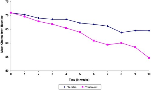
Figure 2. Change in visual acuity – test drug prevents patients from vision decline.

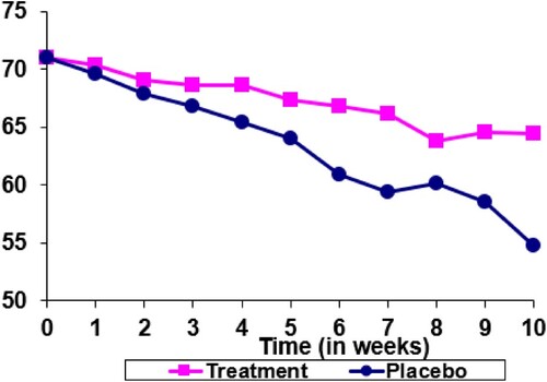
In Figure 2, the test drug is developed to preserve vision. Patients with the eye disease experience vision loss over time. If a patient receives placebo, the visual acuity reduces from 70 to 55 up to the week 10 visit (the blue curve). The test drug helps reduce the decline in vision and the patient treated with test drug experiences a change in visual acuity from 70 to 65 up to week 10 visit (the pink curve). Now that the placebo patient drops out at visit 7 with the last available visual acuity at 60. If both the test drug treated patient and the placebo treated patient complete the 10 week treatment, a treatment difference of 10 (65 – 55) can be observed. However, because of the drop out of the placebo treated patient, the last observation analysis provides a treatment difference of 5 (65 – 60). Now, the LOCF is conservative.

Therefore, to criticize last observation analysis being overly conservative, or possibly anti-conservative, is not appropriate. The performance of LOCF analysis with respect to conservativeness depends on the setting and the background of the specific clinical trial.

Next to look at the second criticism of LOCF – point estimate being biased. Of course if in a four week clinical trial, and the primary parameter is set at the week 4 visit, then the last observation analysis would provide a biased point estimate. However, in clinical practice when a physician makes diagnosis and prescription decisions, how can the drug developer help? The communication tool a drug developer (together with the regulatory agency) uses to guide the prescription practice is the drug label. Hence the question is whether the week 4 visit information, or the last observation analysis, should be provided in the drug label in order to help with prescription considerations.

In medical practice, for a physician to care a patient, one of the most critical steps is to make a correct diagnosis. After the diagnosis is established, the physician would consider a most appropriate treatment to help the patient. At this point, the physician recalls other patients with similar diagnosis and their responses to the prescribed treatments. Then, based on those patients' experiences, the physician makes a prescription decision. This thinking process is about the last observation from previous patients. It has nothing to do with the week 4 visit. Therefore, the drug label should describe patient experiences from the last observation, not from the week 4 visit. In a clinical trial with four weekly visits, the primary parameter that serves the medical purposes should be last observation, not week 4 visit.

When statisticians talk about bias, the term ‘bias’ is the difference between the estimated value, and the parameter of interest. If the drug label uses last observation to describe the clinical trial results, then the parameter of interest in clinical trials should be last observation, not the week 4 visit. The most appropriate unbiased analysis is the last observation or the LOCF analysis. In fact, based on experiences of analysing longitudinal data in clinical trials, it is apparent that the inter-subject variability is higher than the intra-subject variability – differences among patients are much greater than different measurements collected from the same patient. For the purpose of understanding treatment efficacy, analysing data with equal weight across every patient is a lot more meaningful, than to argue which visit to be used (whether last observation or week 4 visit). In other words, the debate of whether the parameter of interest should be week 4 or last observation is relatively unimportant. The critical point is to respect this ‘one patient, one vote’ principle.

Regarding the third criticism of last observation analysis – under estimation of variability, it originated from lack of understanding of LOCF. The fundamental thinking of last observation analysis includes ‘one patient, one vote’ – each patient contributes one piece of information, and ITT – report data from all participating patients. There is no imputation. In the example of a clinical trial with four weekly visits, if the patient drops out after week 2, then the last observation uses the week 2 data for analysis. Note that this is not a ‘carry forward’ analysis. If people think of carrying forward (LOCF), that means the week 3 visit and week 4 visit are all imputed with the week 2 visit values. If this is the case, of course the true variabilities of visit 3 and visit 4 are not represented and hence resulted with an underestimation of variability. However, this is not what the last observation analysis is about. Therefore, this criticism is based on a misunderstanding of last observation analysis. In public health, the concern is patient care. The delivery of patient care is the medical profession. Statistics should provide support to the medical profession and should respect medical practices. It should be noted that the ‘week 4 visit’ dominates data analysis. The objective of applied statistics is to solve real world problems, and there is not much practical foundation of criticizing last observation analysis. In addition to the three criticisms of LOCF as stated above, there could be one more disadvantage of LOCF application – LOCF uses only one data point in a set of longitudinal data. In order to overcome this disadvantage, an sAUC analysis is proposed in the ‘Implementation’ section of this paper.

Beginning in the mid to late 1990s, people criticize the last observation analysis. They also attempted to introduce alternatives. After turning to the new millennium, one recommendation becoming popular was the mixed model with repeated measures (MMRM). The idea of MMRM received more attention in the early years of this century and some drug submission documents applied MMRM as the primary analysis. However, when these drugs were approved, the approval documents used LOCF as the primary analysis. Therefore, in 2008, the Pharmaceutical Research and Manufacturing Association (PhRMA) of US published a paper (Mallinckrodt et al., 2008) to make clear that drug developers preferred to use MMRM. This publication led FDA authors to publish another paper (Siddiqui et al., 2009) in 2009 to agree that MMRM can be acceptable. After 2009, most of the new drug submission documents employed MMRM as the primary analysis.

This shift from last observation analysis to MMRM exposes this analytical model under more close inspections. Based on the 2008 PhRMA paper, MMRM is expressed as a vector and matrix equation $Y_i=X_{i}a+Z_i{b}_i+{ϵ}_i,$where

1. $Y_i$ is a vector of changes from baseline to each visit for subject i,

2. $a$ is a column vector of fixed effects,

3. $X_i$ is a design (incidence) matrix relating the observations of the i-th subject to a,

4. $b_i$ is a column vector of random effects,

5. $Z_i$ is a design (incidence) matrix relating the observations of the i-th subject to $b_i$, and

6. ${ϵ}_i$ is a column vector of random errors.

For the fixed effect, this model includes

Fixed effect treatment,

Fixed effect investigator site,

Fixed categorical effect visit,

Treatment by visit interaction,

Fixed covariate baseline,

and baseline by visit interaction.

The random effect can be expressed as $\mathrm{V}\mathrm{a}\mathrm{r}\left(Y_i\right)=V=\mathrm{V}\mathrm{a}\mathrm{r}(Z_i{b}_i+{ϵ}_i)=\mathrm{V}\mathrm{a}\mathrm{r}\left(Z_i{b}_i\right)+\mathrm{V}\mathrm{a}\mathrm{r}\left({ϵ}_i\right)=Z_{i}G{Z}_i^{\prime }+R_i.$

In data analysis, suppose the clinical trial is a four week study. Then MMRM considers the primary efficacy time point would be the week 4 visit. In other words, treatments are compared with the week 4 visit means (instead of last observation means). MMRM is a specific application of the general linear mixed effect model. That means, if the model deviates from the above specification, then it can still be a linear mixed model, but may not be an MMRM. For example, in the specification of fixed effect, if the visit effect is considered as a continuous predictor, instead of a categorical effect, then this model is no longer MMRM. Such a model would generally be referred to as a random slope model.

Note that given the above specification, the treatment by visit interaction term is an important predictor in the MMRM. Without this interaction term, the model assumption could be too strong – it would be assumed that the treatment difference between test drug and control stays the same across visits. Again, in the example of a clinical trial with four weekly visits, suppose the comparison is a test drug against placebo. Then there would be eight mean responses – each visit with two means (test drug and placebo control) – four visits provide eight observed mean values. Without interaction, that implies the mean differences between test drug and placebo at visit 1 is the same as the treatment difference at visit 2, the same as visit 3, and the same as visit 4. This assumption would be too strong. In practice, a study team designs the clinical trial with four weekly visits because the team believes that the treatment difference in visit 2 could be greater than the difference of visit 1. The difference of visit 3 is greater than that of visit 2 and finally visit 4 provides the largest separation between test drug and placebo. In this case, the interaction term is critical to be included into MMRM because without this term, the assumption would be too strong.

However, it is also this treatment by visit interaction that causes concerns in treatment comparisons. One advantage MMRM claims is that it ‘took all observations into consideration, not simply the last observation’. Without this interaction term, of course all visits are included in the estimate of treatment effect. But if this interaction term is introduced in the model, then the contributions of visits 1, 2, and 3 to the visit 4 estimate become limited. In fact, this interaction term makes the MMRM efficacy estimate more like the week 4 responses. In treatment comparisons, MMRM compares treatment effect at week 4 visit, and it causes the MMRM to become more similar to the completer analysis, and less likely to be the last observation analysis. Clearly, MMRM violates the ‘one patient, one vote’ principle because patients with week 4 visits contribute to treatment comparison much more than those patients without the week 4 visit.

It is known that completer analysis is biased because it violates the ITT principle. If MMRM is closer to a completer analysis, then use of MMRM as primary analysis for drug approval could be problematic. As stated above, MMRM violates the ‘one patient, one vote’ principle. From a drug approval point of view, the scientific foundation is based on the statistical hypothesis testing framework – if the test drug mean is far apart from the placebo mean, so far away that the p-value is less than alpha, then the drug can be approved. The key question is ‘what does this treatment group mean’. In the LOCF analysis, this is the mean of last observation from each patient. This estimator is well understood by both physicians and statisticians. In the completer analysis, this is the mean of the fourth visit. However, when there is missing data, it is not clear what MMRM is estimating.

Completer analysis violates the ITT principle, and MMRM violates ‘one patient, one vote’ principle. Last observation analysis satisfies both principles, and is the only unbiased estimator when that is the parameter to be used in drug label. Also, it is not clear what MMRM is estimating. Given these difficulties associated with MMRM, the International Council for Harmonization (ICH) proposed to revisit this problem about longitudinal data analysis and published a draft guidance document – ICH E9 (R1) in 2017. This guidance (ICH E9 (R1), 2019) was finalized in 2019.

3. ICH E9 (R1)

The objective of ICH E9 (R1) is to combine the analysis population, the efficacy endpoint, and sensitivity analyses into an integrated framework. It also attempts to improve interdisciplinary communication and to be inclusive. This document introduces two new ideas – intercurrent events and estimand. Both need close interdisciplinary communications.

Regarding interdisciplinary communications, there are at least the following three sets of communications in drug development and new drug approval – (1) communications between statisticians and physicians within the sponsor that develops this new drug; (2) communications between statisticians and physicians within the regulatory agency (e.g., FDA); and (3) communications between the sponsor and the agency. In certain situations, another set of communications can also be helpful – communications across various therapeutic areas. This can be considered as the fourth set of communications – it can happen within the sponsor, and can happen within regulatory agencies, or both.

Typically, many difficulties came from the first two sets of communications because the thinking process of a physician and a statistician can be very different. The fundamental task for medical practice is about patient care. Therefore, the training and education of a medical school emphasize on how to understand a patient's condition, and make the best diagnosis, as well as prescribing the best treatment for this patient. On the other hand, a statistician is trained to think of a population. Because it is not feasible to study the entire population, the general practice is to take a sample from the population, and to make inferences about the population using the samples on hand. Consequently, an individual patient only contributes one piece of data from a statistical point of view. Under a continuous distribution, one piece of data has a measure zero – $P[X=x]=0$. Therefore, the major difficulty in communications between physicians and statisticians is that a physician views a patient as an individual, as a single person, while a statistician views each data point as a piece of information. Therefore, in order to clarify this misunderstanding, it is important to remind statisticians that randomization is performed on patients, not visits. In data analysis, the focus should be on patients, not visits.

One important topic that ICH E9 (R1) brought up is the concept of intercurrent events. Actually, this is about missing data or missing visits. Fundamentally speaking, there are only two types of intercurrent events – one type is that the visits or the data are not available (data are missing – patient did not return, lack of efficacy, experiencing adverse events, death, or other reasons); another type is that the data is observed and collected (data are not missing), but cannot be used for the primary clinical efficacy analysis. This second type of intercurrent events is mostly about patients use of alternative treatment (e.g., a rescue medication, a medication prohibited by the protocol, or a subsequent line of therapy). For the second type, statisticians need to work with physicians in order to arrive at a mutual understanding – communication is the key.

As stated at beginning of this section, the objective of ICH E9 (R1) is to combine the analysis population, the efficacy endpoint, and sensitivity analyses into an integrated framework. In fact, the term ‘estimand’ reflects the combination of analysis population, efficacy endpoint, and sensitivity analysis. Regarding estimand, ICH E9 (R1) proposes five strategies:

1. Treatment policy strategy,

2. Composite strategy,

3. Hypothetical strategy,

4. Principal stratum strategy, and

5. While on treatment strategy.

Note that other than (3) (hypothetical strategy), every other strategy follows the ‘one patient, one vote’ principle.

In fact, the treatment policy strategy has been applied in practice before. This used to be thought of as a method of ‘retrieve dropouts’. In the past, for certain diseases, the clinical study protocol would require each patient to return to the clinic for a final visit, regardless whether the patient dropped out, or completed the entire clinical trial duration. On this basis, each patient would contribute a final visit in the trial, and the final analysis can be performed using this primary time point to serve as the efficacy variable. However, even if the protocol is specified for retrieve dropouts, there can still be patients failing to return at the final clinic visit. When this was the case, the typical implementation used to be the last observation analysis.

The composite strategy mostly applies to time to event endpoint or binary endpoint. One example could be found in a long-term cardiovascular clinical trial that the primary efficacy endpoint is time to a major cardiovascular event. A major cardiovascular event can be stroke, myocardial infarction, hospitalization for cardiovascular causes, or death because of cardiovascular-related complications. If a patient did not experience any of the above event up to the protocol specified time of follow-up, the patient is considered censored. This primary efficacy endpoint is an example of a composite endpoint. Of course overall survival, progression free survival, event free survival, and many other time to event endpoints used in oncology studies can all be thought of as examples under the composite strategy. This clearly follows the ‘one patient, one vote’ principle.

The while on treatment strategy is the same as the last observation analysis. As discussed above, this is one of the most useful endpoints used for approval of many very good drugs for about four decades. Clearly, it is ‘one patient, one vote’, and satisfies ITT.

The principal stratum strategy can be thought of as the completer analysis (or the observed cases analysis). This analysis does not satisfy ITT and it can mostly serve as a supportive analysis or sensitivity analysis. However, it follows the ‘one patient, one vote’.

Finally, the hypothetical strategy allows most of the MMRM or other complicate modelling. It does not satisfy the ‘one patient, one vote’ principle, and it is closer to the completer analysis.

Based on this understanding, the ICH E9 (R1) guidance document reflects a basic spirit of being inclusive. It allows both the principal stratum strategy (violates ITT) and hypothetical strategy (violates ‘one patient, one vote’) to be acceptable. In clinical trial applications, for the purpose of protecting alpha, in specifying the primary endpoint, there can only be one single primary model for data analysis. If more than one model is specified as primary, then the alpha can no longer be preserved. Therefore, a reasonable recommendation could be that the primary estimand is the while on treatment strategy. Then consider the principal stratum or hypothetical strategy as supportive. In this ICH E9 (R1) guidance, the basic philosophy that primary efficacy analysis needs to follow both the ‘one patient, one vote’ and the ITT principle should be relatively clear.

4. Implementation

In the treatment policy strategy and the while on treatment strategy, the implementation of ‘one patient, one vote’ can be straightforward – the last observation or LOCF analysis would be appropriate. However, there is more flexibility for the while on treatment strategy. Using this strategy, there are at least three additional ways to take advantage of data collected before the last visit – use of slope, average over time, and standardized area under curve (sAUC, Ting et al., 2021). Details of these three additional ways of implementing while on treatment strategy are covered in this section.

If the project team is willing to assume that the responses over time follow a straight line, then a simple linear regression can be applied to summarize responses of each patient. The linear regression provides an intercept estimate and a slope estimate for the corresponding patient, and the mean slope of each treatment group can be calculated. For statistical comparison of treatment groups, a two sample t test or an ANCOVA model can be applied to analyse the slopes obtained from each patient. Note that from the general linear mixed models view point, one application is known as the random slope model. In actual data analysis, the use of this random slope model may not be appropriate because the treatment comparisons obtained from that general model may not reflect this ‘one patient, one vote’ principle. The reason is that in estimating treatment means, the parameter estimate $\hat{\theta }$ is calculated based on matrix operations – $\hat{\theta }=(X^{\mathrm{\top }}X{)}^{-1}{X}^{\mathrm{\top }}Y$. In this operation, when the number of observations from each patient is different, the ‘mean slope’ calculated can be different from the two-step procedure described above (obtain individual slope using simple regression first, then perform t-test or ANCOVA). The recommended way of analysis of slopes is the two-step method, instead of the linear mixed (or random slope) model approach, in order to achieve ‘one patient, one vote’.

The second alternative of implementing while on treatment strategy using all of the observations is the simple mean over time. Suppose there are three post baseline time points denoted as $t_1$, $t_2$, and $t_3$. At each time point there is a response observation Y. Denote these observations as $Y_1$, $Y_2$, and $Y_3$, correspondingly. Let the baseline value be $Y_0$, and the mean over time is simply $\overline{Y}=(Y_1+Y_2+Y_3)/3$. The estimator of interest is mean change from baseline or that the primary endpoint is $\overline{Y}-Y_0$. Because this simple mean estimator is easy to understand, and easy to interpret, it has been used in practical applications.

Finally, a third way of data analysis under while on treatment strategy is the sAUC approach. Area under the curve (AUC) is a very popular method in summarizing measurements observed over time. Again, suppose there are three time points denoted as time $t_1$, $t_2$, and $t_3$. At each time point there is a response observation Y, and denote these observations as $Y_1$, $Y_2$, and $Y_3$, correspondingly. Plot these six points such that time is on the x-axis and response is on the y-axis. Then the four points ($t_1$, 0), ($t_1$, $Y_1$), ($t_2$, $Y_2$), and ($t_2$, 0), formulate a trapezoid. The area under $Y_1$ and $Y_2$ between time $t_1$ and $t_2$ can be calculated as $(t_2-t_1)\times (Y_1+Y_2)/2$. Similarly, the area under y values between time $t_2$ and $t_3$ can be computed as $(t_3-t_2)\times (Y_2+Y_3)/2$. Add these two trapezoidal areas to get the area under the curve over these three time points ($t_1$, $t_2$, and $t_3$).

For example, if a test drug is developed to lower systolic blood pressure (SBP), then a Phase II or III clinical trial would have to be designed with an objective to compare the test drug against the placebo control. Suppose this is a four-week study, and SBP is measured during weekly outpatient visits. The hypothesis is to test whether the primary variable (the primary endpoint) is statistically significant. In this example, five SBP measures are observed from each patient – week 0 (SBP taken before randomization, or the baseline measurement), weeks 1, 2, 3, and 4. After end of the study, an AUC can be calculated for each patient – if a patient completes all four weeks, then the AUC for this patient is computed by adding areas between weeks 0 and 1, between weeks 1 and 2, between weeks 2 and 3, and finally between weeks 3 and 4. Sum of these four trapezoidal areas provides the AUC for the given patient.

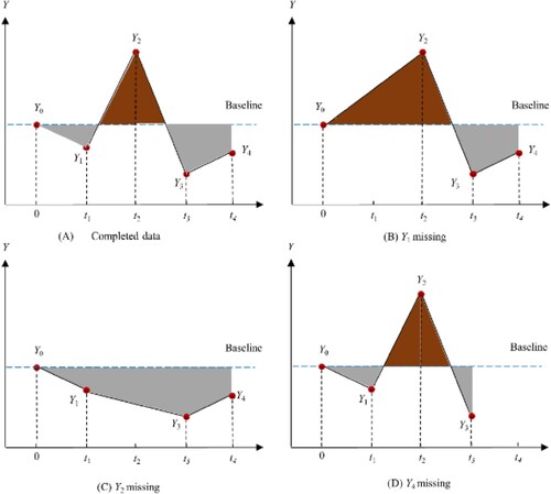
The standardized area under curve (sAUC) is obtained from dividing the AUC (as calculated from above) by total time used in the computation of this AUC, and then subtracting the baseline measure. In Figure 3, panel (A), if the AUC is calculated using all observations taken from time points 0, $t_1$, $t_2$, $t_3$, and $t_4$, the AUC is calculated from time 0 to $t_1$, from $t_1$ to $t_2$, from $t_2$ to $t_3$, and from $t_3$ to $t_4$. After obtaining this AUC, divide it by $t_4$ (time $t_4$ – time 0), minus the time 0 (baseline) measurement ($Y_0$). Then this value becomes the sAUC value for that patient.

Figure 3. Standardized area under the curve (sAUC).

In pharmacokinetics (PK) applications, one of the important parameters is AUC. The reason that PK analysis does not need to go through the standardization process (divide by total time and subtract from baseline) is that duration of PK data collection is usually short (one or two days), and these data are obtained under intensively supervised environments. On the other hand, longitudinal data observed from clinical trials treating chronic diseases take at least a few weeks, sometimes up to several months or even several years, and, generally, participants are out-patients. Such is a loosely controlled environment. On this basis, the standardization process can be very helpful.

The interpretation of sAUC can be thought of as the ‘average change in the primary endpoint from baseline experienced by the patient.’ This interpretation can be easily understood by both statisticians and non-statisticians. From Figure 3, the baseline value ($Y_0$) is the horizontal dotted line. sAUC is the shaded area divided by time – hence the average change experienced by the patient. Note that if the patient's efficacy response is decreased, then the sAUC is a negative value. Otherwise, it is positive. From Figure 1, the difference between the areas with dark colour and areas with light colour divided by time can be thought of as the sAUC. In panel (A) of Figure 3, the sAUC reflects average change from baseline, up to time $t_4$, without missing data. If $Y_1$ is missing, then panel (B) provides a larger positive value than panel (A). However, if $Y_2$ is missing, then the average change becomes negative, as shown in panel (C). Finally, when $Y_4$ is missing in panel (D), the average change takes a positive value.

There is only one key assumption to call sAUC as the average change over time: changes between any two consecutively observed values are linear. In most practical applications, this assumption can easily be satisfied. In other words, sAUC is a relatively robust estimate of average change over time for each patient, for the duration while this patient is staying in the given clinical trial whether there is any missing value or not.

For data analysis of a trial with stratified randomization, the well-established statistical model [3] used for analysis of LOCF data can directly be applied for analysing slopes, simple mean over time and sAUC $Y_{ijk}=\mu +{\tau }_i+{\gamma }_j+\text{β}{X}_{ijk}+{ϵ}_{ijk},$where

1. $Y_{ijk}$ is the sAUC from the k-th subject treated by the i-th treatment of the j-th stratum;

2. $\mu$ is the overall mean;

3. ${\tau }_i$ is the effect from the i-th treatment group;

4. ${\gamma }_j$ is the stratification factor effect from the j-th stratum;

5. $\text{β}$ is the slope estimate associated with the baseline covariate;

6. $X_{ijk}$ is the baseline value from the k-th subject treated by the i-th treatement of the j-th stratum;

7. ${ϵ}_{ijk}$ is the residual associated with the k-th subject within the i-th treatment group from the j-th stratum.

The above model is known as the analysis of covariance (ANCOVA). The key assumption in this model is that ${ϵ}_{ijk}$ is independently and identically distributed with mean 0 and variance ${\sigma }^2$. From practical experiences of most continuous data collected from clinical trials, this assumption can be satisfied. Furthermore, this model has been used for drug approval successfully over decades of drug development and regulation. Note that this ANCOVA model is not only applicable under the while on treatment strategy including LOCF, slope, average over time, and sAUC, but also applicable to the treatment policy strategy (last observation analysis), as well as the principal stratum strategy.

5. Discussion

It is well known that ‘data analysis needs to respect statistical design’. In clinical trial design, the fundamental scientific justification comes from randomization. Unit of randomization is patient, not visit. Therefore, in data analysis, the ‘one patient, one vote’ principle should be closely followed. Another key principle – ITT, is also originated from randomization. Therefore, the primary analysis of efficacy in a clinical trial needs to follow both the ‘one patient, one vote’, and the ITT principle. The last observation, or LOCF analysis following both principles, has been used for drug approval between the late 1960s and 2008, very successfully.

In both clinical practice and clinical trials, experiences demonstrate that the inter-subject variability is greater than the intra-subject variability. This is the case regardless how tight the inclusion/exclusion criteria are specified in the protocol. Therefore, in data analysis, understanding and management of inter-subject variability are more important. On this basis, this ‘one patient, one vote’ principle is important. Relatively speaking, the intra-subject variability as compared with the inter-subject variability is much less after that the degree of freedom is considered. If statisticians are concerned about the intra-subject variability, they can apply the slope analysis, average over time, or sAUC. From this point of view, the argument of last observation vs week 4 visit is not really significant. However, this ‘one patient, one vote’ principle is one of the scientific pillars of clinical trials, of drug development and of drug approval. Statisticians must pay attention to this fundamental thinking – without randomization, there is no clinical trial.

In public health, close communications between physicians and statisticians are critical. This is especially true in the clinical development and regulatory review of new drugs. Such communications happen within the sponsoring organization (mostly pharmaceutical companies and biotech industry), within regulatory agencies, and between the sponsor and agency. Over the years, the medical profession emphasized, and re-emphasized that the ‘one patient, one vote’ principle is very important. It takes the statistical profession to pay attention to this view. In other words, the ‘one patient, one vote’ principle is critically important from both the statistical and the medical professions.

This ‘one patient, one vote’ principle has also been reflected in pharmacokinetics (PK) data analysis. In PK studies, drug concentration data are collected over time. This can also be viewed as longitudinal data. However, in analysis of PK data, the PK experts summarize each individual's data (over time) into PK parameters – Cmax, Tmax, AUC, T1/2, Kel, …. PK analysis strictly follows this ‘one patient, one vote’ principle.

Data imputation (Rubin, 2008) could be a useful tool in statistical applications other than clinical development or regulatory review of new drugs. In the approval process of a new drug, there can be controversial issues about drug efficacy and drug safety. From a pharmaceutical company point of view, in defending their scientific foundation, observed data is the best tool. In the defense of issues associated with the study drug, the use of any imputed data puts the drug maker on a soft footing. Arguments based on imputed data cannot provide a solid scientific foundation. In clinical development of new drugs, the best strategy is not to perform any data imputation.

One reason that ICH has to draft and publish the E9 (R1) guidance document is that in the new drug submission and review process, there was confusion about whether MMRM violates the ‘one patient, one vote’ principle. This guidance recognized that for modelling approaches failing to respect the ‘one patient, one vote’ principle, it can only be thought of as ‘hypothetical’. Furthermore, the introduction of intercurrent event in ICH E9 (R1) is attempting to encourage more interdisciplinary communications.

In longitudinal data analysis with continuous response variables, the most useful strategy would be the while on treatment strategy. Historical records are very clear – most of drugs with longitudinal continuous efficacy endpoints have been approved using this strategy for almost four decades before 2009. Additionally, this strategy allows most flexibility – last observation analysis, slope analysis, average over time, and sAUC are all applicable to this strategy. The while on treatment strategy is scientifically sound because it respects both the ITT principle, and the ‘one patient, one vote’ principle. In certain situations when retrieve dropout is sensible, the treatment policy strategy can also be useful. Again, the appropriate implementation of treatment policy strategy would also be the last observation analysis.

For primary analysis of efficacy in clinical trials, the reasonable and scientifically justified strategies include while on treatment strategy, treatment policy strategy, and composite strategy. The principle stratum strategy and hypothetical strategy can be very useful as sensitivity analysis or supportive analysis. The main concern of using the principle stratum strategy as primary analysis is that it violates the ITT principle. The concern of using the hypothetical strategy as primary analysis is that it violates the ‘one patient, one vote’ strategy.

Disclosure statement

No potential conflict of interest was reported by the author(s).

References

- EMA (2011). Guideline on missing data in confirmatory clinical trials. European Medicine Agency. Retrieved from https://www.ema.europa.eu/en/documents/scientific-guideline/guideline-missing-data-confirmatory-clinical-trialsen.pdf
- ICH E9 (1998). Statistical principles for clinical trials. Retrieved from https://database.ich.org/sites/default/files/E9Guideline.pdf
- ICH E9 (R1) (2019). Addendum on estimands and sensitivity analysis in clinical trials to the guideline on statistical principles for clinical trials. Retrieved from https://database.ich.org/sites/default/files/E9-R1S/tep4Guideline20191203.pdf16
- Mallinckrodt, C. H., Lane, P. W., Schnell, D., Peng, Y., & Mancuso, J. P. (2008). Recommendations for the primary analysis of continuous endpoints in longitudinal clinical trials. Drug Information Journal, 42(4), 303–319. https://doi.org/10.1177/009286150804200402
- Rubin, D. B. (2008). Multiple imputation after 18+ years (with discussion). Journal of the American Statistical Association, 91(434), 473–489. https://doi.org/10.1080/01621459.1996.10476908
- Shao, J., & Zhong, B. (2003). Last observation carry-forward and last observation analysis. Statistics in Medicine, 22(15), 2429–2441. https://doi.org/10.1002/(ISSN)1097-0258
- Shao, J., & Zhong, B. (2006). On the treatment effect in clinical trials with dropout. Journal of Biopharmaceutical Statistics, 16(1), 25–33. https://doi.org/10.1080/10543400500406488
- Siddiqui, O., Hung, H. M. J., & O'Neill, R. (2009). MMRM vs LOCF: A comprehensive comparison based on simulation study and 25 NDA datasets. Journal of Biopharmaceutical Statistics, 19(2), 227–246. https://doi.org/10.1080/10543400802609797
- Ting, N., Chen, D., Ho, S., & Capppelleri, J. (2017). Phase II clinical development of new drugs. Springer.
- Ting, N., Huang, L., Deng, Q., & Capppelleri, J. (2021). Average response over time as estimand: An alternative implementation of the while on treatment strategy. Statistics in Biosciences, 13, 479–494. https://doi.org/10.1007/s12561-021-09301-x