Regression models of Pearson correlation coefficient

Abstract

We propose two simple regression models of Pearson correlation coefficient of two normal responses or binary responses to assess the effect of covariates of interest. Likelihood-based inference is established to estimate the regression coefficients, upon which bootstrap-based method is used to test the significance of covariates of interest. Simulation studies show the effectiveness of the method in terms of type-I error control, power performance in moderate sample size and robustness with respect to model mis-specification. We illustrate the application of the proposed method to some real data concerning health measurements.

Keywords:

• Binary responses
• bivariate normal responses
• Pearson correlation coefficient
• regression

1. Introduction

Most regression models have been developed to describe the relationship between the expected value of response(s) and a number of covariates (predictors). In some situations, it is desired to understand the influence of covariates on the strength of Pearson correlation between two responses. For example, in some psychological study, it is of interest to understand the impact of age and/or sex on the association between physical functionality and mental functionality of the elder (Thomas et al., 2016).

One traditional measure for such association is the partial correlation coefficient, i.e., the correlation coefficient of two responses after removing the covariate effect (Anderson, 2003). However, its inference depends on the normality assumption and it misses the connection to the actual values of the covariates which is supposed to have different effects on the association. In terms of the rank-based counterpart, Liu et al. (2018) proposed covariate-adjusted partial Spearman's rank correlation using probability scale residuals, which is particularly useful for ordinal responses.

Another method is to use a conditional approach to assess the correlation at different levels of the covariates. Bartlett (1993) proposed to model the Fish z-transformed correlation by a polynomial regression of a single covariate z. His model builds a linear regression up on paired observations of $(z_k,r(z_k\left)\right)$, $k=1,\dots ,K$, where $r\left(z_k\right)$ is the sample correlation coefficient of two responses at $z_k$ over K distinct levels of z. One clear drawback of this method is that it requires repeated measures of responses at $z_k$, which would lead to the demand of a large total sample size and even larger when multiple covariates are included. Other studies along this direction include Yu and Dunn (1982) and Paul (1989). Wilding et al. (2011) proposed a model to relate a transformed correlation coefficient of two normal responses ($y_1$ and $y_2$) with a linear combination of covariates ($z_1,\dots ,z_p$) through the probit link, i.e., $(1+\rho )/2=\mathrm{\Phi }({\gamma }_0+{\gamma }_1{z}_1+\cdots +{\gamma }_p{z}_p)$, where $\rho =\mathrm{c}\mathrm{o}\mathrm{r}\mathrm{r}(y_1,y_2)$ and Φ is the distribution function of the standard normal variable. (Restricted maximum likelihood corrected LRT is used to test the significance of covariates.) We point out that the linear transformed correlation $(1+\rho )/2$ guarantees the range for a distribution function. However, it can lose efficiency when ρ is known positive (since it can be modelled directly without transformation).

All the aforementioned methods consider the continuous responses. In many situations, there are only binary responses available, e.g., after dichotomization. In this paper, we propose two simple regression models of Pearson correlation coefficient of two normal responses and two binary responses (Section 2). Specifically, when the correlation coefficient is known positive, the logistic link function is used and when the correlation coefficient is arbitrary in $(-1,1)$, the hyperbolic tangent (or Fisher z-transformation) link function is used. Likelihood-based inference is developed to estimate the regression coefficients (Section 3). We demonstrate the performance of the proposed method by simulation in Section 4 and illustrate the applications in great detail to a real data concerning physical functionality and mental functionality of the elder (Section 5). We defer the technical details in Appendix.

2. Model

Let $(y_1,y_2)$ be a pair of responses of a subject with correlation coefficient $\rho =\mathrm{c}\mathrm{o}\mathrm{r}\mathrm{r}(y_1,y_2)$. Let $x_1,\dots ,x_p$ denote p associated covariates of the paired responses, which follow a joint distribution $f(x_1,\dots ,x_p)$. Consider modelling ρ as a monotonic function of the linear combination of these covariates through (1) $\rho =h\left({\mathbf{x}}^{\mathrm{\top }}\text{β}\right),$(1) where $\mathbf{x}=(1,x_1,\dots ,x_p{)}^{\mathrm{\top }}$ and $\text{β}=({\text{β}}_0,{\text{β}}_1,\dots ,{\text{β}}_p{)}^{\mathrm{\top }}$. When $\rho >0$, we use the logistic function $h\left(x\right)=(1+{\mathrm{e}}^{-\mathrm{x}}{)}^{-1}$, referred by link 1. When $-1<\rho <1$, we use the hyperbolic tangent function $h\left(x\right)=\tanh \left(x\right)=({\mathrm{e}}^{2\mathrm{x}}-1)/({\mathrm{e}}^{2\mathrm{x}}+1)$, referred by link 2. We adopt these two commonly used link functions to map the real line to intervals $(0,1)$ and $(-1,1)$, respectively, as they are analytically simple. Other links can also be used, e.g., the probit link for $\rho >0$. When the correlation is known positive, the logistic function is preferred as it is more efficient for estimation and easy for interpretation. Let $h^{\prime }$ and $h^{″}$ denote the first and second derivatives of h, respectively. Our goal is to assess model (1(1) $\rho =h\left({\mathbf{x}}^{\mathrm{\top }}\text{β}\right),$(1) ).

2.1. Bivariate normal responses

Assume that $y_1$ and $y_2$ follow a bivariate normal distribution with marginal distributions $N({\mu }_1,{\sigma }_1^2)$ and $N({\mu }_2,{\sigma }_2^2)$, respectively. For j = 1, 2, we further model the expected value of $y_j$ by a linear regression, i.e., $\mathrm{E}(y_j\mid \mathbf{x})={\mu }_j={\mathbf{x}}^{\mathrm{\top }}{\mathit{\gamma }}_j$ where ${\mathit{\gamma }}_j=({\gamma }_0,{\gamma }_1,\dots ,{\gamma }_p{)}^{\mathrm{\top }}$. Denote $\mathit{\eta }=({\mathit{\gamma }}_1^{\mathrm{\top }},{\mathit{\gamma }}_2^{\mathrm{\top }},{\sigma }_1^2,{\sigma }_2^2{)}^{\mathrm{\top }}$ as the collection of all nuisance parameters.

The log-likelihood function is (2) $\ell (\text{β},\mathit{\eta })=-\log \left(2\text{π}\right)-\frac{T_1}{2(1-{\rho }^2)}+\frac{\rho T_2}{1-{\rho }^2}-\frac{\log (1-{\rho }^2)}{2},$(2) where (3) $T_1={\left(\frac{y_1-{\mu }_1}{{\sigma }_1}\right)}^2+{\left(\frac{y_2-{\mu }_2}{{\sigma }_2}\right)}^2,T_2=\frac{(y_1-{\mu }_1)(y_2-{\mu }_2)}{{\sigma }_1{\sigma }_2},$(3) $\rho =h\left({\mathbf{x}}^{\mathrm{\top }}\text{β}\right)$, and ${\mu }_j={\mathbf{x}}^{\mathrm{\top }}{\mathit{\gamma }}_j$. The first and second derivatives of ℓ with respect to $\text{β}$ are, respectively (4) $\mathit{s}(\text{β},\mathit{\eta })=\left\{a\right(\rho )T_1+b(\rho )T_2+c(\rho \left)\right\}\mathbf{x},H(\text{β},\mathit{\eta })=\left\{u\right(\rho )T_1+v(\rho )T_2+w(\rho \left)\right\}\mathbf{x}{\mathbf{x}}^{\mathrm{\top }},$(4) where a, b, c, u, v and w are given in Table 1. By the fact that $\mathrm{E}(T_1\mid \mathbf{x})=2$ and $\mathrm{E}(T_2\mid \mathbf{x})=\rho$, we have $\mathrm{E}\left(\mathit{s}\right)=\mathbf{0}$, where $\mathbf{0}$ is the zero vector.

Table 1. Some functions under two link functions.

	Link 1	Link 2
$h\left(x\right)$	$(1+{\mathrm{e}}^{-\mathrm{x}}{)}^{-1}$	$\tanh \left(x\right)$
$h^{\prime }\left(x\right)$	$h\left(x\right)\{1-h(x\left)\right\}$	$\{1+h(x\left)\right\}\{1-h(x\left)\right\}$
$h^{″}\left(x\right)$	$h\left(x\right)\{1-h(x\left)\right\}\{1-2h(x\left)\right\}$	$-2h\left(x\right)\{1+h(x\left)\right\}\{1-h(x\left)\right\}$
a	$-{\displaystyle \frac{{\rho }^2}{(1-\rho )(1+\rho {)}^2}}$	${\displaystyle \frac{-\rho }{(1-\rho )(1+\rho )}}$
b	${\displaystyle \frac{(1+{\rho }^2)\rho }{(1-\rho )(1+\rho {)}^2}}$	${\displaystyle \frac{(1+{\rho }^2)}{(1-\rho )(1+\rho )}}$
c	${\displaystyle \frac{{\rho }^2}{1+\rho }}$	ρ
u	${\displaystyle \frac{-{\rho }^2(2-\rho +{\rho }^2)}{(1-\rho )(1+\rho {)}^3}}$	${\displaystyle \frac{-(1+{\rho }^2)}{(1-\rho )(1+\rho )}}$
v	$-{\displaystyle \frac{\rho (-1+\rho -5{\rho }^2+{\rho }^3)}{(1-\rho )(1+\rho {)}^3}}$	${\displaystyle \frac{4\rho }{(1-\rho )(1+\rho )}}$
w	${\displaystyle \frac{{\rho }^2(1-\rho )(2+\rho )}{(1+\rho {)}^2}}$	$(1+\rho )(1-\rho )$

2.2. Bivariate binary responses

Assume that both $y_1$ and $y_2$ are binary responses. Let $\mathrm{E}\left(y_1\right)=p_1$ and $\mathrm{E}\left(y_2\right)=p_2$. For a, b = 0, 1, let $I_{ab}=I(y_1=a,y_2=b)$, where $I(\cdot )$ is the indicator function, and $p_{ab}=\mathrm{E}\left(I_{ab}\right)=\mathrm{P}(y_1=a,y_2=b)$. Clearly, $p_{00}+p_{01}+p_{10}+p_{11}=1$. By definition, we have $p_1=p_{11}+p_{10},p_2=p_{11}+p_{01},\rho =\frac{p_{11}-p_1{p}_2}{\sqrt{p_1(1-p_1)p_2(1-p_2)}}.$ Inversely, given $p_1$, $p_2$ and ρ, we can obtain (5) $p_{11}=p_1{p}_2+\rho \sqrt{p_1(1-p_1)p_2(1-p_2)},p_{10}=p_1-p_{11},p_{01}=p_2-p_{11}.$(5) For j = 1, 2, we further model the expected value of $y_j$ by a logistic regression through $p_j=\{1+\exp (-{\mathbf{x}}^{\mathrm{\top }}{\mathit{\gamma }}_j){\}}^{-1}$, where ${\mathit{\gamma }}_j$ is as defined in Section 2.1. Denote $\mathit{\eta }=({\mathit{\gamma }}_1^{\mathrm{\top }},{\mathit{\gamma }}_2^{\mathrm{\top }}{)}^{\mathrm{\top }}$. (Through (1(1) $\rho =h\left({\mathbf{x}}^{\mathrm{\top }}\text{β}\right),$(1) ) and (5(5) $p_{11}=p_1{p}_2+\rho \sqrt{p_1(1-p_1)p_2(1-p_2)},p_{10}=p_1-p_{11},p_{01}=p_2-p_{11}.$(5) ), $p_{ab}$ is a function of $(\text{β},\mathit{\eta })$.)

By (5(5) $p_{11}=p_1{p}_2+\rho \sqrt{p_1(1-p_1)p_2(1-p_2)},p_{10}=p_1-p_{11},p_{01}=p_2-p_{11}.$(5) ), the log-likelihood is $\ell (\text{β},\mathit{\eta })=\sum _{a,b=0,1}{I}_{ab}\log p_{ab}=\sum _{a,b=0,1}{I}_{ab}\log (c_{ab}+d_{ab}\rho ),$ where $\begin{array}{rl}{c}_{11}& =p_1{p}_2,d_{11}=\sqrt{p_1(1-p_1)p_2(1-p_2)},\\ c_{10}& =p_1(1-p_2),d_{10}=-d_{11},\\ c_{01}& =p_2(1-p_1),d_{01}=-d_{11},\\ c_{00}& =(1-p_1)(1-p_2),d_{00}=d_{11}.\end{array}$ Then, the first and second derivatives of ℓ with respect to $\text{β}$ are, respectively (6) $\mathit{s}(\text{β},\mathit{\eta })=\sum _{a,b=0,1}{I}_{ab}{e}_{ab}\left(\rho \right)\mathbf{x},H(\text{β},\mathit{\eta })=\sum _{a,b=0,1}{I}_{ab}{f}_{ab}\left(\rho \right)\mathbf{x}{\mathbf{x}}^{\mathrm{\top }},$(6) where $e_{ab}\left(\rho \right)=\frac{d_{ab}{h}^{\prime }\left({\mathbf{x}}^{\mathrm{\top }}\text{β}\right)}{c_{ab}+d_{ab}\rho },f_{ab}\left(\rho \right)=\frac{-d_{ab}^2{h}^{\prime 2}\left({\mathbf{x}}^{\mathrm{\top }}\text{β}\right)+d_{ab}(c_{ab}+d_{ab}\rho )h^{″}\left({\mathbf{x}}^{\mathrm{\top }}\text{β}\right)}{(c_{ab}+d_{ab}\rho {)}^2}.$ The detailed expressions of $e_{ab}$ and $f_{ab}$ under the two models of h are given in Appendix. When $\mathrm{E}(I_{ab}\mid \mathbf{x})=p_{ab}$, we have $\mathrm{E}\left(\mathit{s}\right)=\mathbf{0}$.

3. Inference

Let $\left\{\right(y_1,y_2,x_1,\dots ,x_p):i=1,\dots ,n\}$ denote independent samples of $(y_1,y_2,x_1,\dots ,x_p)$ of size n. For $i=1,\dots ,n$ and j = 1, 2, denote ${\mathbf{x}}_i=(1,x_{i1},\dots ,x_{ip}{)}^{\mathrm{\top }}$, ${\mathbf{y}}_j=(y_{1j},\dots ,y_{nj}{)}^{\mathrm{\top }}$, $\overline{\mathbf{x}}=n^{-1}\sum _{i=1}^n{\mathbf{x}}_i$ and $X_{n\times p}=({\mathbf{x}}_1,\dots ,{\mathbf{x}}_n{)}^{\mathrm{\top }}$.

The gradient (first derivative) and the Hessian matrix (second derivative) of the log-likelihood over n independent samples with respect to $\text{β}$ are $\mathit{s}(\text{β},\mathit{\eta })=\sum _{i=1}^n{\mathit{s}}_i(\text{β},\mathit{\eta })$ and $H(\text{β},\mathit{\eta })=\sum _{i=1}^n{H}_i(\text{β},\mathit{\eta })$, respectively, where ${\mathit{s}}_i(\text{β},\mathit{\eta })$ and $H_i(\text{β},\mathit{\eta })$ are obtained by replacing $(y_1,y_2,\mathbf{x})$ in (4(4) $\mathit{s}(\text{β},\mathit{\eta })=\left\{a\right(\rho )T_1+b(\rho )T_2+c(\rho \left)\right\}\mathbf{x},H(\text{β},\mathit{\eta })=\left\{u\right(\rho )T_1+v(\rho )T_2+w(\rho \left)\right\}\mathbf{x}{\mathbf{x}}^{\mathrm{\top }},$(4) ) or (6(6) $\mathit{s}(\text{β},\mathit{\eta })=\sum _{a,b=0,1}{I}_{ab}{e}_{ab}\left(\rho \right)\mathbf{x},H(\text{β},\mathit{\eta })=\sum _{a,b=0,1}{I}_{ab}{f}_{ab}\left(\rho \right)\mathbf{x}{\mathbf{x}}^{\mathrm{\top }},$(6) ) by $(y_{i1},y_{i2},{\mathbf{x}}_i)$ for the ith subject.

In addition, let $G_i(\text{β},\mathit{\eta })={\mathrm{\partial }}^2{\ell }_i/\mathrm{\partial }\text{β}\mathrm{\partial }{\mathit{\eta }}^{\mathrm{\top }}$. Denote $\mathrm{\Theta }=\mathrm{E}\left(H_i\right)$ and $\mathbf{J}=\mathrm{E}\left(G_i\right)$, where the expectation is taken with respect to the joint distribution of $(y_{i1},y_{i2},{\mathbf{x}}_i)$. Let $\mathbf{I}=\mathrm{E}\left\{{\mathit{s}}_i\right(\text{β},\mathit{\eta }\left){\mathit{s}}_i^{\mathrm{\top }}\right(\text{β},\mathit{\eta }\left)\right\}$ denote the Fisher information matrix with respect to $\text{β}$. It is noted that unlike the usual regression of the mean value of response, the regularity condition does not hold for the model (1(1) $\rho =h\left({\mathbf{x}}^{\mathrm{\top }}\text{β}\right),$(1) ) (Tsiatis, 2006, Theorem 3.2). (It can be easily verified that $\mathbf{I}\ne -\mathrm{\Theta }$.)

Let $\hat{\mathit{\eta }}$ be the maximum likelihood estimate (MLE) of $\mathit{\eta }$ obtained from the marginal models. For instance, the marginal MLEs of the nuisance parameters under the bivariate normal response case are ${\hat{\mathit{\gamma }}}_j=(X^{\mathrm{\top }}X{)}^{-1}{X}^{\mathrm{\top }}{\mathbf{y}}_j$, ${\hat{\sigma }}_j^2=n^{-1}\sum _{i=1}^n(y_{ji}-{\hat{\mu }}_{ji}{)}^2$, where ${\hat{\mu }}_{ji}={\mathbf{x}}_i^{\mathrm{\top }}{\hat{\mathit{\gamma }}}_j$. By large sample theory, we have $\hat{\mathit{\eta }}\stackrel{p}{\to }\mathit{\eta }$ and $\sqrt{n}(\hat{\mathit{\eta }}-\mathit{\eta })\stackrel{d}{\to }N(\mathbf{0},{\mathrm{\Sigma }}_{\eta })$, where ${\mathrm{\Sigma }}_{\eta }$ is the covariance matrix.

Next, we estimate $\text{β}$ by using the Newton–Raphson method through iterating (7) ${\text{β}}^{(r+1)}={\text{β}}^{\left(r\right)}-H^{-1}({\text{β}}^{\left(r\right)},\hat{\mathit{\eta }})\mathit{s}({\text{β}}^{\left(r\right)},\hat{\mathit{\eta }}),$(7) where ${\text{β}}^{\left(r\right)}$ is the estimate of $\text{β}$ at the rth iteration. The convergence of Newton–Raphson method depends on the initial point and the negative definitiveness of the Hessian matrix, which guarantees the (unique) global maximizer of the log-likelihood function. The initial estimate ${\text{β}}^{\left(1\right)}$ can be chosen such that $h\left({\overline{\mathbf{x}}}^{\mathrm{\top }}{\text{β}}^{\left(1\right)}\right)$ is in the range of ρ. However, the Hessian matrix involves the plug-in estimators of the nuisance parameters. It is not trivial to show its negative definitiveness theoretically. Nevertheless, numerical study shows the condition holds with all eigenvalues being negative. Denote the root of the Newton–Raphson method by $\widehat{\text{β}}$.

Theorem 3.1

Suppose that the conditions of Lemma A.1 for the bivariate normal responses or those of Lemma A.2 for the bivariate binary responses hold. $($Lemmas A.1 and A.2 are given in Appendix.$)$ Suppose the iteration (7(7) ${\text{β}}^{(r+1)}={\text{β}}^{\left(r\right)}-H^{-1}({\text{β}}^{\left(r\right)},\hat{\mathit{\eta }})\mathit{s}({\text{β}}^{\left(r\right)},\hat{\mathit{\eta }}),$(7) ) converges. (i) $\widehat{\text{β}}$ is a consistent estimator of $\text{β}$, i.e., $\widehat{\text{β}}\stackrel{p}{\to }\text{β}$, and (ii) $\sqrt{n}(\widehat{\text{β}}-\text{β})\stackrel{d}{\to }N(\mathbf{0},\mathrm{\Sigma })$, where Σ is the covariance matrix given in the proof.

The significance of the overall model is assessed by testing the hypothesis $H_0:{\text{β}}_1=\cdots ={\text{β}}_p=0$. Denote the Wald statistic $W={\widehat{\text{β}}}_{-0}^{\mathrm{\top }}{\widehat{\mathrm{c}\mathrm{o}\mathrm{v}}}^{-1}\left({\widehat{\text{β}}}_{-0}\right){\widehat{\text{β}}}_{-0}$, where ${\widehat{\text{β}}}_{-0}=({\widehat{\text{β}}}_1,\dots ,{\widehat{\text{β}}}_p{)}^{\mathrm{\top }}$ and $\widehat{\mathrm{c}\mathrm{o}\mathrm{v}}\left({\widehat{\text{β}}}_{-0}\right)$ is the estimate of the covariance of ${\widehat{\text{β}}}_{-0}$. By Theorem 3.1, under the null hypothesis, W follows a chi-square distribution of degrees of freedom p asymptotically. The significance of individual covariate $x_j$ ($j=1,\dots ,p$) is assessed by testing the hypothesis $H_{0j}:{\text{β}}_j=0$ using the statistic $w_j={\widehat{\text{β}}}_j/\widehat{\mathrm{s}\mathrm{e}}\left({\widehat{\text{β}}}_j\right)$, where $\widehat{\mathrm{s}\mathrm{e}}\left({\widehat{\text{β}}}_j\right)$ is the estimate of the standard deviation of ${\widehat{\text{β}}}_j$, which is the square root of the $(j,j)$th element of $\widehat{\mathrm{c}\mathrm{o}\mathrm{v}}\left({\widehat{\text{β}}}_{-0}\right)$. The null distribution of $w_j$ is asymptotically standard normal. Since the exact expression of Σ is rather complicated, we use bootstrap to estimate it in practice.

4. Simulation study

We conduct simulations to examine the performance of the proposed model for making inference in estimation and testing.

4.1. Setup

Unlike possible large numbers of covariates for the mean model, a small number of relevant covariates are usually adequate for modelling the correlation coefficient. Consider the number of covariates p to be two and three, respectively. Set the sample size n to be 100, 200, 400 and 1000, respectively.

For bivariate normal responses, set the marginal variances ${\sigma }_1^2={\sigma }_2^2=1$. For both bivariate normal responses and bivariate binary responses, we set both ${\mathit{\gamma }}_1$ and ${\mathit{\gamma }}_2$ to be a vector of p + 1 zeros for the marginal mean models. It simplifies the data generation without simplifying the estimation procedure. Let $x_1,\dots ,x_p$ be independent uniform random variables in (0,1).

For the correlation coefficient model, set ${\text{β}}_0=0.25$. Under the nonnull model, set ${\text{β}}_1$,…,${\text{β}}_p$ under two link functions as in Table 2, where only the first covariate is significant. Under the null model, simply set all ${\text{β}}_1,\dots ,{\text{β}}_p$ to be zeros. We set $(0.25,0,\dots ,0)$ as the initial values for $\text{β}$ under both link functions.

Table 2. Specifications of ${\text{β}}_1,\dots ,{\text{β}}_p$ under p = 2, 3 and two link functions.

	$({\text{β}}_1,{\text{β}}_2)$	$({\text{β}}_1,{\text{β}}_2,{\text{β}}_3)$
Link 1	$(1,0)$	$(1,0,0)$
Link 2	$(-1,0)$	$(-1,0,0)$

Throughout, we set the significant level to be 0.05 for both the global test and individual test, and set the number of replications, B, to be 1000.

4.2. Results

First, denote the empirical root of mean square error of $\widehat{\text{β}}$ by $\mathrm{E}\mathrm{R}\mathrm{M}\mathrm{S}\mathrm{E}=B^{-1}\sum _{b=1}^B\left\{\sum _{j=0}^p\right({\widehat{\text{β}}}_j^{\left(b\right)}-{\text{β}}_j{)}^2{\}}^{1/2}$, where ${\widehat{\text{β}}}^{\left(b\right)}$ is the estimate of $\text{β}$ in the bth replication. It measures the performance of the estimation in terms of magnitude. Second, denote the directional consistency rate (CR) by $\mathrm{C}\mathrm{R}=B^{-1}\sum _{b=1}^B\left\{n^{-1}\sum _{i=1}^{n}I\right({\hat{\rho }}_i^{\left(b\right)}{\rho }_i^{\left(b\right)}>0\left)\right\}$, where ${\rho }_i^{\left(b\right)}$ is the true correlation coefficient in the bth replication and ${\hat{\rho }}_i^{\left(b\right)}=h\left({\mathbf{x}}_i^{\mathrm{\top }}{\widehat{\text{β}}}^{\left(b\right)}\right)$. It measures the performance of estimation in terms of sign direction.

Table 3 presents the type-I error of the global test and individual tests under the null model. It is seen that the proposed resampling test controls the type-I error well at the nominal level.

Table 3. Type-I errors (in %) of the global test (for the model significance) and individual test (for the significance of the covariates) under two types of responses, two link functions and various sample sizes.

			p = 2			p = 3
Response	Link	n	Global	${\text{β}}_1$	${\text{β}}_2$	Global	${\text{β}}_1$	${\text{β}}_2$	${\text{β}}_3$
Normal	1	100	2.5	2.6	2.3	1.6	2.6	2.1	2.4
		200	4.5	5.1	3.9	3.7	4.2	3.0	3.9
		400	5.5	4.3	5.0	4.1	3.8	3.8	5.8
		1000	6.0	4.4	5.4	5.8	5.1	5.3	5.3
	2	100	5.6	4.3	5.2	6.6	5.2	5.3	4.7
		200	5.7	3.9	6.3	7.5	6.0	6.3	5.3
		400	6.1	6.1	5.5	5.5	5.1	3.7	5.1
		1000	5.7	4.6	4.6	4.5	4.0	5.0	4.7
Binary	1	100	2.6	2.5	2.5	4.6	3.5	3.5	4.4
		200	0.1	0.8	1.0	0.1	0.5	0.6	0.4
		400	1.1	2.2	2.1	0.3	1.8	2.9	1.4
		1000	5.5	5.2	6.1	4.4	3.7	5.8	4.7
	2	100	0.6	1.1	1.2	0.5	0.9	0.8	0.7
		200	3.7	3.3	3.9	3.3	4.1	5.0	3.7
		400	4.9	5.1	4.0	4.9	4.8	5.1	6.3
		1000	5.1	4.6	4.6	5.6	5.5	4.7	6.1

Columns 4–5 and 9–10 of Table 4 present the ERMSE and CR under the nonnull model considered in Section 4.1. It is seen that as the sample size increases the ERMSE decreases while the CR increases as expected. The CR ranges from 85% to 100% indicating that the proposed model yields a good fit in the sign direction of the correlation coefficient. Columns 7–9 and 12–15 of Table 4 present the powers of the global test and individual tests of the covariates. It is seen that both the global test and the individual test for the significant covariate (i.e., $x_1$) gain power as the sample size increases as desired. The rejection rates for the insignificant covariates (i.e., $x_2$ and $x_3$) are close to the nominal level as desired. We note that the power performance depends on the actual model. In general, we see the proposed method works well under moderate sample size.

Table 4. ERMSE, CR and testing power of β's of models considered in Table 1 with various sample sizes.

			p = 2					p = 3
					Power					Power
Model	Link	n	RMSE	CR(%)	Global	${\text{β}}_1$	${\text{β}}_2$	RMSE	CR(%)	Global	${\text{β}}_1$	${\text{β}}_2$	${\text{β}}_3$
Normal	1	100	1.149	100	15.0	18.7	7.8	1.296	100	14.5	18.6	13.5	13.2
		200	0.848	100	36.2	43.5	6.0	1.039	100	29.6	40.8	7.9	8.0
		400	0.619	100	69.4	75.8	6.3	0.737	100	63.2	77.1	5.4	5.8
		1000	0.373	100	98.6	99.3	4.8	0.447	100	97.4	99.0	4.3	5.1
	2	100	0.583	87.1	69.0	77.4	4.7	0.74	85.1	60.0	68.4	4.6	3.3
		200	0.401	90.5	95.5	97.5	5.4	0.493	89.1	94.0	97.3	4.6	4.8
		400	0.274	93.5	100	100	5.3	0.336	92.3	100	100	5.7	5.1
		1000	0.165	96.0	100	100	5.9	0.207	95.3	100	100	5.1	4.6
Binary	1	100	2.924	100	6.0	7.0	4.7	3.529	100	10.5	10.1	8.7	8.8
		200	1.766	100	2.9	5.7	1.8	2.319	100	2.8	6.3	2.0	1.3
		400	1.066	100	7.0	16.5	1.5	1.337	100	3.1	13.8	1.2	1.2
		1000	0.620	100	52.5	68.8	3.8	0.772	100	38.9	69.3	3.3	2.9
	2	100	0.696	86.2	20.8	40.7	1.6	0.871	83.9	4.7	26.1	0.7	0.6
		200	0.443	89.8	90.4	94.8	3.8	0.556	88.4	80.5	94.4	4.8	4.7
		400	0.308	93	99.7	99.7	4.7	0.367	91.7	99.6	100	4.4	4.6
		1000	0.196	95.5	99.9	99.9	5.1	0.235	94.8	100	100	5.0	5.0

4.3. Sensitivity analysis

We adopt the simulation model from Wilding et al. (2011) for bivariate normal responses, where $y_1\sim N(1+2x_1,1)$, $y_2\sim N(1.5+1.2x_1,1)$ and their correlation coefficient is given by $\rho (y_1,y_2)=2\mathrm{\Phi }(0.5+{\text{β}}_1{x}_1)-1$ with $x_1$ being a uniform random variable in $(0,1)$. Consider ${\text{β}}_1$ to be 0, 0.5 and 1, respectively, to represent the null case and two nonnull cases. Set n to be 30, 60 and 150, respectively.

We compute the rejection rate for testing the significance of $x_1$ using the proposed method with link 2 in comparison with Wilding et al. (2011)'s method by which the model is correctly specified. This serves as a sensitivity analysis under model mis-specification. Table 5 reports the rejection rates under the considered cases. It is seen that under the null case when ${\text{β}}_1=0$ the proposed method controls the type-I error well. Under the nonnull cases when ${\text{β}}_1=0.5$ and 1 the proposed method is less powerful than Wilding et al.'s method when the sample size is 30 and becomes comparable in power when the sample size gets larger ($⩾60$).

Table 5. Rejection rates (in %) of Wilding et al. (2011)'s method and the proposed method for testing the significance of the covariate.

n	${\text{β}}_1$	Wilding et al.	Proposed
30	0	6.1	4.4
	0.5	10.6	7.2
	1	31.5	13.6
60	0	5.2	4.8
	0.5	17.2	17.1
	1	56.2	53.6
150	0	5.3	6.1
	0.5	43.2	41.8
	1	95.3	95.5

5. Real data application

Our data are taken from the survey of National Health Measurement Study in 2005–2006 (Fryback, 2009). It collects responses to health-related quality of life questionnaires and health status questions through Short Form SF-36 questionnaires from 3844 older adults in the continental United States (1641 males and 2203 females).

5.1. Bivariate normal responses

First, we illustrate the application of the proposed model to the bivariate normal responses case. The SF-36 items were aggregated into eight health concepts, which were further summarized into the physical component summary (PCS) and the mental component summary (MCS), both in the range of $(0,100)$ with higher scores indicating better physical and mental health functions, respectively [28]. Several medical studies showed that the PCS declined significantly with age, but that the MCS did not change with age (Kim, 2016; Ware Jr et al., 1994). To continue along these lines, we applied the proposed method to further investigate the effect of gender and marital status. We used the Fisher z-transformation (i.e., tanh link) to accommodate negative value of correlation. The estimate model for the correlation between PCS and age is found to be $\tanh \left(\rho \right(\mathrm{P}\mathrm{C}\mathrm{S},\mathrm{a}\mathrm{g}\mathrm{e}\left)\right)=-0.203-0.145\times \mathrm{M}\mathrm{A}\mathrm{R}\mathrm{R}\mathrm{I}\mathrm{E}\mathrm{D}+0.018\times \mathrm{S}\mathrm{E}\mathrm{X},$ where MARRIED is 1 if married or living with a partner and 0 otherwise, and SEX is 1 if female and 0 if male. The corresponding p-values for marital status and gender are $<0.001$ and 0.592, respectively, indicating strong significance of marriage and insignificance of gender. The negative coefficient of MARRIED implies that the status of being married or living with a partner aggravates the declination of PCS with age ($-0.283$ for people married or living with a partner and $-0.209$ for people living by themselves). In other words, the people who are married or living with a partner have relatively lower physical functionality than the people who live by themselves when they age in general. On the other hand, our model concurred with the conclusion of insignificant correlation between MCS and age. In addition, neither gender nor marital status has significant effect on this correlation. (The details are omitted.)

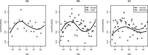
Moreover, we applied the proposed model to study the age effect on the correlation of PCS and MCS. (Throughout this section the observations of age are standardized, denoted by AGE${}^{\ast }$, before fitting the model as covariate.) Insignificant result is found and supported by the visual inspection of the correlations over 20 age intervals determined by the percentiles (Figure 1(a)). This result is different from the finding of Wilding et al. (2011), who showed a nonlinear downward trend of the correlation coefficient over age based on the 2003–2004 Health Outcome Survey data. When we further include gender and marital status as covariates, there is no significant gender effect either (p-value 0.312) as also seen in Figure 1(b). However, there appears a very mild effect of marital status (p-value 0.236) in the way that the status of being married or living with a partner slightly reduces the correlation from otherwise slight positive to the level of near zero (Figure 1(c)). (The fitted model is $\tanh \left(\rho \right(\mathrm{P}\mathrm{C}\mathrm{S},\mathrm{M}\mathrm{C}\mathrm{S}\left)\right)=0.148-0.016\times {\mathrm{A}\mathrm{G}\mathrm{E}}^{\ast }-0.063\times \mathrm{M}\mathrm{A}\mathrm{R}\mathrm{R}\mathrm{I}\mathrm{E}\mathrm{D}-0.052\times \mathrm{S}\mathrm{E}\mathrm{X}$.)

Figure 1. (a) Correlation of PCS and MCS over 20 age groups, (b) correlation of PCS and MCS over 20 age groups with different genders, (c) correlation of PCS and MCS over 20 age groups with different marital status.

5.2. Bivariate binary responses

Second, we applied the proposed method to model the correlation of two binary indicators of stroke (STR) and diabetes (DIA) using the covariates of age, gender and marital status. Since the correlation is known positive, the logistic link is used. The estimated model which includes the second-order age effect is $\begin{array}{rl}\mathrm{l}\mathrm{o}\mathrm{g}\mathrm{i}\mathrm{s}\mathrm{t}\mathrm{i}\mathrm{c}\left(\rho \right(\mathrm{S}\mathrm{T}\mathrm{R},\mathrm{D}\mathrm{I}\mathrm{A}\left)\right)=& -2.050-1.352\times {\mathrm{A}\mathrm{G}\mathrm{E}}^{\ast }-0.090\times {\mathrm{A}\mathrm{G}\mathrm{E}}^{\ast 2}\\ & +0.938\times \mathrm{M}\mathrm{A}\mathrm{R}\mathrm{R}\mathrm{I}\mathrm{E}\mathrm{D}+0.270\times \mathrm{S}\mathrm{E}\mathrm{X}\end{array}$ with strong significance of the linear age effect (p-value $<0.001$) 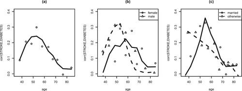and marriage effect (p-value 0.028) and insignificance of the second-order term of age (p-value 0.786) and gender effect (p-value 0.675). It is seen from Figure 2(a) that the correlation exhibits a parabola shape in age where the largest value (about 0.25) occurs around age 55 and then starts to decline afterwards. This indicates that the association of stroke and diabetes is strongly age dependent. The diabetes becomes a less significant risk factor to stroke after a certain age, e.g., 70 (Kim, 2016). The status of married or living with a partner contributes significantly to the positive correlation (0.145 for married vs 0.106 for otherwise) especially for people who are more than 50 years old (Figure 2(c)), which could be explained by the evidence of low physical functionality found before.

Figure 2. (a) Correlation of STROKE and DIABETES over 10 age groups, (b) correlation of STROKE and DIABETES over 10 age groups with different genders, (c) correlation of STROKE and DIABETES over 10 age groups with different marital status.

6. Concluding remarks

We propose two simple regression models of Pearson correlation coefficient of two continuous responses or two binary responses. Likelihood-based inference is developed to estimate the model and test the significance of covariates. Our method for the binary response case is new to the literature and is useful for analysing data when outcomes are observed in binary form (such as yes or no) as seen in many psychological and sociological studies. The proposed method is easy to implement and computationally affordable. (The Newton–Raphson iteration converges in a few steps.) We have made R package available upon request.

It is noted that for the binary response case, the correlation ρ actually has a restricted range given by $max\{-{\psi }_1{\psi }_2,-({\psi }_1{\psi }_2{)}^{-1}\}⩽\rho ⩽min\{{\psi }_1{\psi }_2^{-1},{\psi }_2{\psi }_1^{-1}\}$, where ${\psi }_1=\sqrt{p_1/(1-p_1)}$ and ${\psi }_2=\sqrt{p_2/(1-p_2)}$ (Qaqish, 2003). A more precise model than the Fisher z-transformation is warranted to further improve the efficiency.

The limitation of the present paper is that the proposed method does not handle the case of mixed responses, i.e., one continuous response and one binary response, or more generally an ordinal response categorized from a latent variable, such as ‘mild’, ‘moderate’, ‘severe’. Regression model of correlation involving latent variable(s) is worth investigation. We will report the result in a separate work.

Disclosure statement

All authors declare no conflict of interest.

Data availability statement

The data that support the findings of this study are available from the corresponding author upon request.

Appendix. Technical details

A.1. Details of $e_{ab}$ and $f_{ab}$

The expressions of $e_{ab}$ and $f_{ab}$ under two link functions of h are, respectively $e_{ab}\left(\rho \right)=\{\begin{array}{ll}{\displaystyle \frac{d_{ab}\rho (1-\rho )}{c_{ab}+d_{ab}\rho },}& \mathrm{l}\mathrm{i}\mathrm{n}\mathrm{k}1,\\ {\displaystyle \frac{d_{ab}(1+\rho )(1-\rho )}{c_{ab}+d_{ab}\rho },}& \mathrm{l}\mathrm{i}\mathrm{n}\mathrm{k}2,\end{array}$ and $f_{ab}\left(\rho \right)=\{\begin{array}{ll}{\displaystyle \frac{\{-d_{ab}^2+d_{ab}(c_{ab}+d_{ab}\rho )(1-2\rho \left)\right\}{\rho }^2(1-\rho {)}^2}{(c_{ab}+d_{ab}\rho {)}^2},}& \mathrm{l}\mathrm{i}\mathrm{n}\mathrm{k}1,\\ {\displaystyle \frac{\{-d_{ab}^2-d_{ab}(c_{ab}+d_{ab}\rho \left)2\rho \right\}(1+\rho {)}^2(1-\rho {)}^2}{(c_{ab}+d_{ab}\rho {)}^2},}& \mathrm{l}\mathrm{i}\mathrm{n}\mathrm{k}2.\end{array}$

A.2. Lemmas

Lemma A.1

Assume that under the bivariate normal response model in Section 2.1, there exist constants $c_1$, $c_2$, $c_3$, and $c_4$ such that $0<c_1⩽|\rho |⩽c_2<1$, $0⩽|{\hat{\mu }}_j|<c_3$, $|{\hat{\sigma }}_j|⩾c_4>0$ for j = 1, 2. Then, (i) $n^{-1}\sum _{i=1}^n{H}_i({\text{β}}^{\ast },\hat{\mathit{\eta }})\stackrel{p}{⟶}\mathrm{\Theta }$, and (ii) $n^{-1}\sum _{i=1}^n{G}_i(\text{β},{\mathit{\eta }}^{\ast })\stackrel{p}{⟶}\mathbf{J}$.

Proof.

Note that we cannot apply the weak law of large number as ${\ell }_i({\text{β}}^{\ast },\hat{\mathit{\eta }})$s and ${\ell }_i(\text{β},{\mathit{\eta }}^{\ast })$s are neither independent nor identically distributed.

(i) Let ${\hat{T}}_{1i}=(\frac{y_{1i}-{\hat{\mu }}_{1i}}{{\hat{\sigma }}_1}{)}^2+(\frac{y_{2i}-{\hat{\mu }}_{2i}}{{\hat{\sigma }}_2}{)}^2$ and ${\hat{T}}_{2i}=\frac{(y_{1i}-{\hat{\mu }}_{1i})(y_{2i}-{\hat{\mu }}_{2i})}{{\hat{\sigma }}_1{\hat{\sigma }}_2}$. First, by the assumptions of $0⩽|{\hat{\mu }}_j|<c_3$ and $|{\hat{\sigma }}_j|⩾c_4>0$ for j = 1, 2, we have $\begin{array}{rl}\left|{\hat{T}}_{1i}\right|& =|{\left(\frac{y_{1i}-{\hat{\mu }}_1}{{\hat{\sigma }}_1}\right)}^2+{\left(\frac{y_{2i}-{\hat{\mu }}_2}{{\hat{\sigma }}_2}\right)}^2|⩽\frac{y_{1i}^2+c_3^2+2c_3|y_{1i}|}{c_4^2}+\frac{y_{2i}^2+c_3^2+2c_3|y_{2i}|}{c_4^2};\\ \left|{\hat{T}}_{2i}\right|& =\left|\frac{(y_{1i}-{\hat{\mu }}_1)(y_{2i}-{\hat{\mu }}_2)}{{\hat{\sigma }}_1{\hat{\sigma }}_2}\right|⩽\frac{(|y_{1i}|+c_3)(|y_{2i}|+c_3)}{c_4^2}.\end{array}$ Second, by the assumption of $0<c_1⩽|\rho |⩽c_2<1$, there exists a positive constant $M_1$ such that $|u\left(\rho \right)|$, $|v\left(\rho \right)|$, and $|w\left(\rho \right)|$ are all bounded by $M_1$. Since $H_i(\text{β},\hat{\mathit{\eta }})=\left\{u\right({\rho }_i){\hat{T}}_{1i}+v({\rho }_i){\hat{T}}_{2i}+w({\rho }_i\left)\right\}{\mathbf{x}}_i{\mathbf{x}}_i^{\mathrm{\top }}$, then, there exists a function $g(\mathbf{x},y)$ such that $\parallel H_i(\text{β},\hat{\mathit{\eta }})\parallel ⩽g({\mathbf{x}}_i,y_i)$ and $\mathrm{E}\left\{g\right({\mathbf{x}}_i,y_i\left)\right\}⩽\mathrm{\infty }$, where $\parallel \cdot \parallel$ is the Euclidean norm (i.e., $\parallel A\parallel =\left\{\mathrm{t}\mathrm{r}\right(A{A}^{\mathrm{\top }}){\}}^{1/2}$). Clearly, $H_i(\text{β},\mathit{\eta })$ is continuous in $({\text{β}}^{\mathrm{\top }},{\mathit{\eta }}^{\mathrm{\top }}{)}^{\mathrm{\top }}$.

By Lemma 2.4 of Newey and McFadden (1994), we have $\underset{\text{β},\mathit{\eta }}{sup}\Vert n^{-1}\sum _{i=1}^n{H}_i(\text{β},\mathit{\eta })-\mathrm{\Theta }\Vert \stackrel{p}{⟶}0$. Since ${\text{β}}^{\ast }\stackrel{p}{⟶}\text{β}$ (because $\widehat{\text{β}}\stackrel{p}{⟶}\text{β}$ and ${\text{β}}^{\ast }$ is between $\text{β}$ and $\widehat{\text{β}}$), $\hat{\mathit{\eta }}\stackrel{p}{⟶}\mathit{\eta }$ and Θ is continuous in $({\text{β}}^{\mathrm{\top }},{\mathit{\eta }}^{\mathrm{\top }}{)}^{\mathrm{\top }}$, by Tsiatis (2006, Section 3.2), the result of (i) follows.

(ii) By (2(2) $\ell (\text{β},\mathit{\eta })=-\log \left(2\text{π}\right)-\frac{T_1}{2(1-{\rho }^2)}+\frac{\rho T_2}{1-{\rho }^2}-\frac{\log (1-{\rho }^2)}{2},$(2) ) and (3(3) $T_1={\left(\frac{y_1-{\mu }_1}{{\sigma }_1}\right)}^2+{\left(\frac{y_2-{\mu }_2}{{\sigma }_2}\right)}^2,T_2=\frac{(y_1-{\mu }_1)(y_2-{\mu }_2)}{{\sigma }_1{\sigma }_2},$(3) ), we have $\begin{array}{rl}\frac{\mathrm{\partial }{T}_{1i}}{\mathrm{\partial }{\mathit{\gamma }}_1^{\mathrm{\top }}}& =-\frac{2(y_{1i}-{\mu }_1)}{{\sigma }_1^2}{\mathbf{x}}_i^{\mathrm{\top }},\frac{\mathrm{\partial }{T}_{2i}}{\mathrm{\partial }{\mathit{\gamma }}_1^{\mathrm{\top }}}=-\frac{y_{2i}-{\mu }_2}{{\sigma }_1{\sigma }_2}{\mathbf{x}}_i^{\mathrm{\top }},\\ \frac{\mathrm{\partial }{T}_{1i}}{\mathrm{\partial }{\mathit{\gamma }}_2^{\mathrm{\top }}}& =-\frac{2(y_{2i}-{\mu }_2)}{{\sigma }_2^2}{\mathbf{x}}_i^{\mathrm{\top }},\frac{\mathrm{\partial }{T}_{2i}}{\mathrm{\partial }{\mathit{\gamma }}_2^{\mathrm{\top }}}=-\frac{y_{1i}-{\mu }_1}{{\sigma }_1{\sigma }_2}{\mathbf{x}}_i^{\mathrm{\top }},\\ \frac{\mathrm{\partial }{T}_{1i}}{\mathrm{\partial }{\sigma }_1^2}& =-\frac{(y_{1i}-{\mu }_1{)}^2}{{\sigma }_1^4},\frac{\mathrm{\partial }{T}_{2i}}{\mathrm{\partial }{\sigma }_1^2}=-\frac{(y_{1i}-{\mu }_1)(y_{2i}-{\mu }_2)}{2{\sigma }_1^3{\sigma }_2},\\ \frac{\mathrm{\partial }{T}_{1i}}{\mathrm{\partial }{\sigma }_2^2}& =-\frac{(y_{2i}-{\mu }_2{)}^2}{{\sigma }_2^4},\frac{\mathrm{\partial }{T}_{2i}}{\mathrm{\partial }{\sigma }_2^2}=-\frac{(y_{1i}-{\mu }_1)(y_{2i}-{\mu }_2)}{2{\sigma }_1{\sigma }_2^3},\end{array}$ and $\begin{array}{rl}\frac{{\mathrm{\partial }}^2{\ell }_i(\text{β},\mathit{\eta })}{\mathrm{\partial }\text{β}\mathrm{\partial }{\mathit{\gamma }}_1^{\mathrm{\top }}}& =\{-a(\rho )\frac{2(y_{1i}-{\mu }_1)}{{\sigma }_1^2}-b(\rho \left)\frac{y_{2i}-{\mu }_2}{{\sigma }_1{\sigma }_2}\right\}{\mathbf{x}}_i{\mathbf{x}}_i^{\mathrm{\top }},\\ \frac{{\mathrm{\partial }}^2{\ell }_i(\text{β},\mathit{\eta })}{\mathrm{\partial }\text{β}\mathrm{\partial }{\mathit{\gamma }}_2^{\mathrm{\top }}}& =\left\{a\right(\rho )\frac{2(y_{2i}-{\mu }_2)}{{\sigma }_2^2}-b(\rho \left)\frac{y_{1i}-{\mu }_1}{{\sigma }_1{\sigma }_2}\right\}{\mathbf{x}}_i{\mathbf{x}}_i^{\mathrm{\top }},\\ \frac{{\mathrm{\partial }}^2{\ell }_i(\text{β},\mathit{\eta })}{\mathrm{\partial }\text{β}\mathrm{\partial }{\sigma }_1^2}& =\left\{a\right(\rho )\frac{(y_{1i}-{\mu }_1{)}^2}{{\sigma }_1^4}-b(\rho \left)\frac{(y_{1i}-{\mu }_1)(y_{2i}-{\mu }_2)}{2{\sigma }_1^3{\sigma }_2}\right\}{\mathbf{x}}_i,\\ \frac{{\mathrm{\partial }}^2{\ell }_i(\text{β},\mathit{\eta })}{\mathrm{\partial }\text{β}\mathrm{\partial }{\sigma }_2^2}& =\{-a(\rho )\frac{(y_{2i}-{\mu }_2{)}^2}{{\sigma }_2^4}-b(\rho \left)\frac{(y_{1i}-{\mu }_1)(y_{2i}-{\mu }_2)}{2{\sigma }_1{\sigma }_2^3}\right\}{\mathbf{x}}_i.\end{array}$ By the assumptions, we can find a function $k(\mathbf{x},y)$ such that $\Vert D_i(\text{β},\mathit{\eta })\Vert ⩽k({\mathbf{x}}_i,y_i)$ and $\mathrm{E}\left\{|k\right({\mathbf{x}}_i,y_i\left)|\right\}<\mathrm{\infty }$. And $D_i(\text{β},\mathit{\eta })$ is continuous in $({\text{β}}^{\mathrm{\top }},{\mathit{\eta }}^{\mathrm{\top }}{)}^{\mathrm{\top }}$. Using the similar argument as in the proof for (i), by Lemma 2.4 of Newey and McFadden (1994) $\underset{\text{β},\mathit{\eta }}{sup}\Vert n^{-1}\sum _{i=1}^n{G}_i(\text{β},\mathit{\eta })-\mathbf{J}\Vert \stackrel{p}{⟶}0$. Since ${\mathit{\eta }}^{\ast }\stackrel{p}{⟶}\mathit{\eta }$ and $\mathbf{J}$ is continuous in $({\text{β}}^{\mathrm{\top }},{\mathit{\eta }}^{\mathrm{\top }}{)}^{\mathrm{\top }}$, the result of (ii) follows.

Lemma A.2

Assume that under the bivariate Bernoulli response model in Section 2.2 there exist constants $d_1,\dots ,d_6$ such that $|h^{\prime }\left({\mathbf{x}}^{\mathrm{\top }}\text{β}\right)|⩽d_1$, $|h^{″}\left({\mathbf{x}}^{\mathrm{\top }}\text{β}\right)|⩽d_2$ for all $\mathbf{x}$, $0<d_3<p_j<d_4<1$, for j = 1, 2, $0<d_5<|\rho |<d_6<1$. Then, (i) $n^{-1}\sum _{i=1}^n{H}_i({\text{β}}^{\ast },\hat{\mathit{\eta }})\stackrel{p}{⟶}\mathrm{\Theta }$, and (ii) $n^{-1}\sum _{i=1}^n{G}_i(\text{β},{\mathit{\eta }}^{\ast })\stackrel{p}{⟶}\mathbf{J}$.

Proof.

(i) By the assumptions, there exists $M_2$ such that $|f_{iab}(\text{β},\mathit{\eta })|⩽M_2$ for all a, b = 0, 1 and $i=1,\dots ,n$. Then, there exists a function $g(\mathbf{x},y)$ such that $\Vert H_i(\text{β},\hat{\mathit{\eta }})\Vert ⩽g_1({\mathbf{x}}_i,y_i)$ and $\mathrm{E}\left\{g_1\right({\mathbf{x}}_i,y_i\left)\right\}⩽\mathrm{\infty }$. Clearly, $H_i(\text{β},\mathit{\eta })$ is continuous in $({\text{β}}^{\mathrm{\top }},{\mathit{\eta }}^{\mathrm{\top }}{)}^{\mathrm{\top }}$. By Lemma 2.4 of Newey and McFadden (1994), $\underset{\text{β},\mathit{\eta }}{sup}\Vert n^{-1}\sum _{i=1}^n{H}_i(\text{β},\mathit{\eta })-\mathrm{\Theta }\Vert \stackrel{p}{⟶}0$.

Since ${\text{β}}^{\ast }\stackrel{p}{⟶}\text{β}$, $\hat{\mathit{\eta }}\stackrel{p}{⟶}\mathit{\eta }$ and Θ is continuous in $({\text{β}}^{\mathrm{\top }},{\mathit{\eta }}^{\mathrm{\top }}{)}^{\mathrm{\top }}$, by Tsiatis (2006) Section 3.2, the result of (i) follows.

(ii) Observe that $\begin{array}{rl}{G}_i(\text{β},\mathit{\eta })& =\sum _{a,b=0,1}{I}_{iab}\frac{\mathrm{\partial }{e}_{iab}(\text{β},\mathit{\eta })}{\mathrm{\partial }{\mathit{\eta }}^{\mathrm{\top }}}{\mathbf{x}}_i\\ & =\sum _{a,b=0,1}{I}_{iab}\frac{\frac{\mathrm{\partial }{d}_{iab}}{\mathrm{\partial }{\mathit{\eta }}^{\mathrm{\top }}}(c_{iab}+d_{iab}{\rho }_i)-(\frac{\mathrm{\partial }{c}_{iab}}{\mathrm{\partial }{\mathit{\eta }}^{\mathrm{\top }}}-\frac{\mathrm{\partial }{d}_{iab}}{\mathrm{\partial }{\mathit{\eta }}^{\mathrm{\top }}}{\rho }_i)d_{iab}}{(c_{iab}+d_{iab}{\rho }_i{)}^2}{h}^{\prime }\left({\mathbf{x}}_i^{\mathrm{\top }}\text{β}\right){\mathbf{x}}_i.\end{array}$ By the logistic model defined in Section 2.2, $\mathrm{\partial }{p}_{ji}/\mathrm{\partial }{\mathit{\eta }}_j^{\mathrm{\top }}=p_j(1-p_j){\mathbf{x}}_i^{\mathrm{\top }}$. The expressions of $\mathrm{\partial }{d}_{iab}/\mathrm{\partial }{\mathit{\eta }}^{\mathrm{\top }}$ and $\mathrm{\partial }{c}_{iab}/\mathrm{\partial }{\mathit{\eta }}^{\mathrm{\top }}$ are obtained as follows. $\begin{array}{rl}\frac{\mathrm{\partial }{d}_{i11}}{\mathrm{\partial }{\mathit{\eta }}_j^{\mathrm{\top }}}& ={\left\{p_{1i}\right(1-p_{1i}\left)p_{2i}\right(1-p_{2i}\left)\right\}}^{1/2}(\frac{1}{2}-p_{ji}){\mathbf{x}}_i^{\mathrm{\top }},j=1,2;\\ \frac{\mathrm{\partial }{d}_{i10}}{\mathrm{\partial }{\mathit{\eta }}_j^{\mathrm{\top }}}& =\frac{\mathrm{\partial }{d}_{i01}}{\mathrm{\partial }{\mathit{\eta }}_j^{\mathrm{\top }}}=-\frac{\mathrm{\partial }{d}_{i11}}{\mathrm{\partial }{\mathit{\eta }}_j^{\mathrm{\top }}},\frac{\mathrm{\partial }{d}_{i00}}{\mathrm{\partial }{\mathit{\eta }}_j^{\mathrm{\top }}}=\frac{\mathrm{\partial }{d}_{i11}}{\mathrm{\partial }{\mathit{\eta }}_j^{\mathrm{\top }}},j=1,2;\\ \frac{\mathrm{\partial }{c}_{i11}}{\mathrm{\partial }{\mathit{\eta }}_j^{\mathrm{\top }}}& =p_{1i}{p}_{2i}(1-p_{ji}){\mathbf{x}}_i^{\mathrm{\top }},j=1,2;\\ \frac{\mathrm{\partial }{c}_{i10}}{\mathrm{\partial }{\mathit{\eta }}_1^{\mathrm{\top }}}& =\frac{\mathrm{\partial }{p}_{1i}}{\mathrm{\partial }{\mathit{\eta }}_1^{\mathrm{\top }}}-p_{2i}\frac{\mathrm{\partial }{p}_{1i}}{\mathrm{\partial }{\mathit{\eta }}_1^{\mathrm{\top }}}=p_{1i}(1-p_{1i})(1-p_{2i}){\mathbf{x}}_i^{\mathrm{\top }};\\ \frac{\mathrm{\partial }{c}_{i10}}{\mathrm{\partial }{\mathit{\eta }}_2^{\mathrm{\top }}}& =-p_{1i}\frac{\mathrm{\partial }{p}_{2i}}{\mathrm{\partial }{\mathit{\eta }}_2^{\mathrm{\top }}}=-p_{1i}{p}_{2i}(1-p_{2i}){\mathbf{x}}_i^{\mathrm{\top }};\\ \frac{\mathrm{\partial }{c}_{i01}}{\mathrm{\partial }{\mathit{\eta }}_1^{\mathrm{\top }}}& =-p_{2i}\frac{\mathrm{\partial }{p}_{1i}}{\mathrm{\partial }{\mathit{\eta }}_1^{\mathrm{\top }}}=-p_{2i}{p}_{1i}(1-p_{1i}){\mathbf{x}}_i^{\mathrm{\top }};\\ \frac{\mathrm{\partial }{c}_{i01}}{\mathrm{\partial }{\mathit{\eta }}_2^{\mathrm{\top }}}& =\frac{\mathrm{\partial }{p}_{2i}}{\mathrm{\partial }{\mathit{\eta }}_2^{\mathrm{\top }}}-p_{1i}\frac{\mathrm{\partial }{p}_{2i}}{\mathrm{\partial }{\mathit{\eta }}_2^{\mathrm{\top }}}=p_{2i}(1-p_{2i})(1-p_{1i}){\mathbf{x}}_i^{\mathrm{\top }};\\ \frac{\mathrm{\partial }{c}_{i00}}{\mathrm{\partial }{\mathit{\eta }}_j^{\mathrm{\top }}}& =-p_{ji}(1-p_{1i})(1-p_{2i}){\mathbf{x}}_i^{\mathrm{\top }},j=1,2.\end{array}$ By the assumptions, we can find a function $\omega (x,y)$ such that $\Vert G_i(\text{β},\mathit{\eta })\Vert ⩽\omega ({\mathbf{x}}_i,y_i)$ and $\mathrm{E}\left\{\omega \right({\mathbf{x}}_i,y_i\left)\right\}<\mathrm{\infty }$. And, $G_i(\text{β},\mathit{\eta })$ is continuous in $({\text{β}}^{\mathrm{\top }},{\mathit{\eta }}^{\mathrm{\top }}{)}^{\mathrm{\top }}$. Using the similar argument as in the proof for (i), by Lemma 2.4 of Newey and McFadden (1994) $\underset{\text{β},\mathit{\eta }}{sup}\Vert n^{-1}\sum _{i=1}^n{G}_i(\text{β},\mathit{\eta })-\mathbf{J}\Vert \stackrel{p}{⟶}0$. Since ${\mathit{\eta }}^{\ast }\stackrel{p}{\to }\mathit{\eta }$ in probability and $\mathbf{J}$ is continuous in $({\text{β}}^{\mathrm{\top }},{\mathit{\eta }}^{\mathrm{\top }}{)}^{\mathrm{\top }}$, the result of (ii) follows.

A.3. Proof of Theorem 3.1

By the standard theory of regression, we have $\sqrt{n}(\hat{\mathit{\eta }}-\mathit{\eta })\to N(0,{\mathrm{\Sigma }}_{\eta })$.

By the fact that $\widehat{\text{β}}$ solves $\mathit{s}(\text{β},\hat{\mathit{\eta }})=\mathbf{0}$, expand $\mathit{s}(\widehat{\text{β}},\hat{\mathit{\eta }})$ (with respect to $\text{β}$) around $\text{β}$ as (A1) $0=\mathit{s}(\widehat{\text{β}},\hat{\mathit{\eta }})=\mathit{s}(\text{β},\hat{\mathit{\eta }})+\sum _{i=1}^n{H}_i({\text{β}}^{\ast },\hat{\mathit{\eta }})(\widehat{\text{β}}-\text{β}),$(A1) where ${\text{β}}^{\ast }$ is between $\widehat{\text{β}}$ and $\text{β}$ component-wise.

Second, expand $\mathit{s}(\text{β},\hat{\mathit{\eta }})$ (with respect to $\mathit{\eta }$) around $\mathit{\eta }$ as (A2) $\mathit{s}(\text{β},\hat{\mathit{\eta }})=\sum _{i=1}^n{\mathit{s}}_i(\text{β},\hat{\mathit{\eta }})=\sum _{i=1}^n{\mathit{s}}_i(\text{β},\mathit{\eta })+\sum _{i=1}^n{G}_i(\text{β},{\mathit{\eta }}^{\ast })(\hat{\mathit{\eta }}-\mathit{\eta }),$(A2) where ${\mathit{\eta }}^{\ast }$ is between $\hat{\mathit{\eta }}$ and $\mathit{\eta }$ component-wise.

Combining (A1(A1) $0=\mathit{s}(\widehat{\text{β}},\hat{\mathit{\eta }})=\mathit{s}(\text{β},\hat{\mathit{\eta }})+\sum _{i=1}^n{H}_i({\text{β}}^{\ast },\hat{\mathit{\eta }})(\widehat{\text{β}}-\text{β}),$(A1) ) and (A2(A2) $\mathit{s}(\text{β},\hat{\mathit{\eta }})=\sum _{i=1}^n{\mathit{s}}_i(\text{β},\hat{\mathit{\eta }})=\sum _{i=1}^n{\mathit{s}}_i(\text{β},\mathit{\eta })+\sum _{i=1}^n{G}_i(\text{β},{\mathit{\eta }}^{\ast })(\hat{\mathit{\eta }}-\mathit{\eta }),$(A2) ), $\sqrt{n}(\widehat{\text{β}}-\text{β})$ is expressed as (A3) $-\sqrt{n}{\left\{\frac{1}{n}\sum _{i=1}^n{H}_i\right({\text{β}}^{\ast },\hat{\mathit{\eta }}\left)\right\}}^{-1}\left[\frac{1}{n}\sum _{i=1}^n{\mathit{s}}_i\right(\text{β},\mathit{\eta })+\left\{\frac{1}{n}\sum _{i=1}^n{G}_i\right(\text{β},{\mathit{\eta }}^{\ast }\left)\right\}(\hat{\mathit{\eta }}-\mathit{\eta }\left)\right].$(A3) By Lemma A.1 for the bivariate normal response case or Lemma A.2 for the bivariate Bernoulli response case, (A4) $\frac{1}{n}\sum _{i=1}^n{H}_i({\text{β}}^{\ast },\hat{\mathit{\eta }})\stackrel{p}{⟶}\mathrm{\Theta }\mathrm{a}\mathrm{n}\mathrm{d}\frac{1}{n}\sum _{i=1}^n{G}_i(\text{β},{\mathit{\eta }}^{\ast })\stackrel{p}{⟶}\mathbf{J}.$(A4) And by the central limit theorem, $n^{-1/2}\sum _{i=1}^n{\mathit{s}}_i(\text{β},\mathit{\eta })\stackrel{d}{⟶}N(\mathbf{0},\mathbf{I})$. Then, by Slusky theorem, (A5) $-{\left\{\frac{1}{n}\sum _{i=1}^n{H}_i\right({\text{β}}^{\ast },\hat{\mathit{\eta }}\left)\right\}}^{-1}\frac{1}{\sqrt{n}}\sum _{i=1}^n{\mathit{s}}_i(\text{β},\mathit{\eta })\stackrel{d}{⟶}N(\mathbf{0},{\mathrm{\Theta }}^{-1}\mathbf{I}{\mathrm{\Theta }}^{-1}),$(A5) and (A6) $-{\left\{\frac{1}{n}\sum _{i=1}^n{H}_i\right({\text{β}}^{\ast },\hat{\mathit{\eta }}\left)\right\}}^{-1}\left\{\frac{1}{n}\sum _{i=1}^n{G}_i\right(\text{β},{\mathit{\eta }}^{\ast }\left)\right\}\sqrt{n}(\hat{\mathit{\eta }}-\mathit{\eta })\stackrel{d}{⟶}N(\mathbf{0},{\mathrm{\Theta }}^{-1}\mathbf{J}{\mathrm{\Sigma }}_{\eta }{\mathbf{J}}^{\mathrm{\top }}{\mathrm{\Theta }}^{-1}).$(A6) Combining (A3(A3) $-\sqrt{n}{\left\{\frac{1}{n}\sum _{i=1}^n{H}_i\right({\text{β}}^{\ast },\hat{\mathit{\eta }}\left)\right\}}^{-1}\left[\frac{1}{n}\sum _{i=1}^n{\mathit{s}}_i\right(\text{β},\mathit{\eta })+\left\{\frac{1}{n}\sum _{i=1}^n{G}_i\right(\text{β},{\mathit{\eta }}^{\ast }\left)\right\}(\hat{\mathit{\eta }}-\mathit{\eta }\left)\right].$(A3) ), (A5(A5) $-{\left\{\frac{1}{n}\sum _{i=1}^n{H}_i\right({\text{β}}^{\ast },\hat{\mathit{\eta }}\left)\right\}}^{-1}\frac{1}{\sqrt{n}}\sum _{i=1}^n{\mathit{s}}_i(\text{β},\mathit{\eta })\stackrel{d}{⟶}N(\mathbf{0},{\mathrm{\Theta }}^{-1}\mathbf{I}{\mathrm{\Theta }}^{-1}),$(A5) ), and (A6(A6) $-{\left\{\frac{1}{n}\sum _{i=1}^n{H}_i\right({\text{β}}^{\ast },\hat{\mathit{\eta }}\left)\right\}}^{-1}\left\{\frac{1}{n}\sum _{i=1}^n{G}_i\right(\text{β},{\mathit{\eta }}^{\ast }\left)\right\}\sqrt{n}(\hat{\mathit{\eta }}-\mathit{\eta })\stackrel{d}{⟶}N(\mathbf{0},{\mathrm{\Theta }}^{-1}\mathbf{J}{\mathrm{\Sigma }}_{\eta }{\mathbf{J}}^{\mathrm{\top }}{\mathrm{\Theta }}^{-1}).$(A6) ), $\sqrt{n}(\widehat{\text{β}}-\text{β})$ is asymptotically normal with zero mean vector and covariance matrix given by $\mathrm{\Sigma }={\mathrm{\Theta }}^{-1}\mathbf{I}{\mathrm{\Theta }}^{-1}+{\mathrm{\Theta }}^{-1}\mathbf{J}{\mathrm{\Sigma }}_{\eta }{\mathbf{J}}^{\mathrm{\top }}{\mathrm{\Theta }}^{-1}+\mathrm{c}\mathrm{o}\mathrm{v}\{\mathrm{L}\mathrm{H}\mathrm{S}\mathrm{o}\mathrm{f}\left(\mathrm{A}5\right),\mathrm{L}\mathrm{H}\mathrm{S}\mathrm{o}\mathrm{f}\left(\mathrm{A}6\right)\}.$

References

- Anderson, T. (2003). An introduction to statistical multivariate analysis. 3rd ed. Wiley.
- Bartlett, R. F. (1993). Linear modelling of Pearson's product moment correlation coefficient: An application of Fisher's z-transformation. Journal of the Royal Statistical Society: Series D, 42(1), 45–53.
- Fryback, D. G. (2009). United States National Health Measurement Study, 2005-2006. Inter-University Consortium for Political and Social Research.
- Kim, D. (2016). Correlation between physical function, cognitive function, and health-related quality of life in elderly persons. Journal of Physical Therapy Science, 28(6), 1844–1848. https://doi.org/10.1589/jpts.28.1844
- Liu, Q., Li, C., Wanga, V., & Shepherd, B. E. (2018). Covariate-adjusted Spearman rank correlation with probability-scale residuals. Biometrics, 74(2), 595–605. https://doi.org/10.1111/biom.v74.2
- Newey, W. K., & McFadden, D. (1994). Large sample estimation and hypothesis testing. Handbook of Econometrics, 4, 2111–2245. https://doi.org/10.1016/S1573-4412(05)80005-4
- Paul, S. (1989). Test for the equality of several correlation coefficients. Canadian Journal of Statistics, 17(2), 217–227. https://doi.org/10.2307/3314850
- Qaqish, B. F. (2003). A family of multivariate binary distributions for simulating correlated binary variables with specified marginal means and correlations. Biometrika, 90(2), 455–463. https://doi.org/10.1093/biomet/90.2.455
- Thomas, P., Jolanda, L., Antonius, J. M. d. C., Joris, P. J. S., & Rudi, G. J. W. (2016). Impact of physical and mental health on life satisfaction in old age: A population based observational study. BMC Geriatrics, 16(1), 194. https://doi.org/10.1186/s12877-016-0365-4
- Tsiatis, A. A. (2006). Semiparametric theory and missing data. Springer.
- Ware Jr, J. E., Kosinski, M., & Keller, S. D. (1994). SF-36 physical and mental summary scales: A user's manual. The Health Institute, New England Medical Center.
- Wilding, G. E., Cai, X., Hutson, A., & Yu, Z. (2011). A linear model-based test for the heterogeneity of conditional correlations. Journal of Applied Statistics, 38(10), 2355–2366. https://doi.org/10.1080/02664763.2011.559201
- Yu, M., & Dunn, O. (1982). Robust tests for the equality of two correlation coefficients: A monte carlo study. Educational and Psychological Measurement, 42(4), 987–1004. https://doi.org/10.1177/001316448204200407