On the MLE of the Waring distribution

Abstract

The two-parameter Waring is an important heavy-tailed discrete distribution, which extends the famous Yule-Simon distribution and provides more flexibility when modelling the data. The commonly used EFF (Expectation-First Frequency) for parameter estimation can only be applied when the first moment exists, and it only uses the information of the expectation and the first frequency, which is not as efficient as the maximum likelihood estimator (MLE). However, the MLE may not exist for some sample data. We apply the profile method to the log-likelihood function and derive the necessary and sufficient conditions for the existence of the MLE of the Waring parameters. We use extensive simulation studies to compare the MLE and EFF methods, and the goodness-of-fit comparison with the Yule-Simon distribution. We also apply the Waring distribution to fit an insurance data.

Keywords:

• Maximum likelihood estimator
• heavy-tailed discrete distribution
• Waring distribution

1. Introduction

The power-law distributions are a class of heavy-tailed univariate distributions that describe a quantity whose probability decreases as a power of its magnitude, which is widely used in social science, network science and so on. Two commonly used discrete examples are Zipf distribution and Yule-Simon distribution (or Yule distribution). Zipf law is found by the linguist Zipf when studying the words in a linguistic corpus, in which the frequency of a certain word is proportional to $r^{-d}$, where r is the corresponding rank and d is some positive value. The Yule-Simon distribution is a highly skewed discrete probability distribution with very long upper tails, named after Udny Yule and Herbert Simon–winner of the 1978 Nobel Prize in economics, with distribution function $P(X=k)=\frac{\alpha \mathrm{\Gamma }\left(k\right)\mathrm{\Gamma }(\alpha +1)}{\mathrm{\Gamma }(\alpha +k+1)},\alpha >0,k=1,2,3,\dots ,$where $\mathrm{\Gamma }(\cdot )$ is the Gamma function, and α is the parameter. Yule (1925) proposed the distribution first, applying it to model the number of species in the biological genera. Simon (1955) rediscovered the ‘Yule’ distribution later, using it to examine city populations, income distributions, and word frequency in publications (Mills, 2017). In Price (1965, 1976), Price, a famous American scientist, found that the number of citations of the literature follows the Yule distribution, when linking the published literature with his cited literature to form a directed network of scientific and technological literature. It is a cumulative advantage distribution based on the mechanism of ‘success breeds success’.

The two-parameter Waring distribution is a generalization of the Yule-Simon distribution, which provides more flexibility than the commonly used one-parameter Zipf distribution, Yule-Simon distribution, negative binomial distribution, etc. The Waring distribution can describe a wide variety of phenomena in actuarial science, network science, library and information science, such as number of shares purchased by each customer, number of traffic accidents, number of nodes in the internet connections, and frequency of authors who publish a certain number of paper (Huete-Morales & Marmolejo-Martín, 2020; Panaretos & Xekalaki, 1986; Seal, 1952; Xekalaki, 1983). The distribution function of $X\sim W(\alpha ,\text{β})$ is given by (1) $P(X=k)=\alpha \cdot \frac{\mathrm{\Gamma }(\text{β}+k-1)}{\mathrm{\Gamma }\left(\text{β}\right)}\cdot \frac{\mathrm{\Gamma }(\alpha +\text{β})}{\mathrm{\Gamma }(\alpha +\text{β}+k)},\alpha >0,\text{β}>0,k=1,2,3,\dots ,$(1) where $\alpha ,\text{β}$ are the parameters of the Waring distribution. It is easy to prove that the Waring distribution is a heavy-tailed distribution, with a polynomial tail of order $\alpha +1$. We can also derive that $E\left(X\right)=1+\frac{\text{β}}{\alpha -1}$ if $\alpha >1$, and $\mathrm{v}\mathrm{a}\mathrm{r}\left(X\right)=\frac{\alpha \text{β}(\alpha +\text{β}-1)}{(\alpha -1{)}^2(\alpha -2)}$ if $\alpha >2$. The Yule-Simon distribution is a special case of the Waring distribution with $\text{β}=1$.

The parameter estimation is extremely important to make a statistical inference. Garcia (2011) provided a fixed-point algorithm to estimate the Yule-Simon distribution parameter. For the Waring distribution, a commonly used method is the EFF (Expectation-First Frequency), which is essentially the method of moments. More specifically, the EFF method uses the sample mean $\overline{X}$ to estimate $E\left(X\right)=1+\frac{\text{β}}{\alpha -1}$ and the empirical first frequency $\hat{P}(X=1)$ to estimate $P(X=1)=\frac{\alpha }{\alpha +\text{β}}$, leading to $\hat{\alpha }=\frac{\hat{P}(X=1)\cdot (\overline{X}-1)}{\hat{P}(X=1)\cdot \overline{X}-1},\widehat{\text{β}}=\frac{\{1-\hat{P}(X=1\left)\right\}\cdot (\overline{X}-1)}{\hat{P}(X=1)\cdot \overline{X}-1}.$The EFF method has two drawbacks: first, it restricts that $\alpha >1$, which can not be used when the first moment does not exist; second, it only uses the information of $P(X=1)$ and $E\left(X\right)$, which loses information of the data. Xekalaki (1985) proposed a factorial moment estimation for the bivariate generalized Waring distribution, which also suffers from these drawbacks.

In the current literature, researchers also considered the maximum likelihood estimator (MLE) of the Waring parameters. However, they usually directly applied the optimization algorithm to the log-likelihood function, without verifying the existence of the MLE (Rivas & Campos, 2021). As we all know, MLE does not exist in all cases. In fact, for some sample data, the MLE of Waring parameters exists, while for some sample data, it does not exist. For example, in the insurance share data analysed in Section 4, the MLE of the Waring parameters does not exist for the groups with central ages 17.5, 22.5 and 67.5; for each group, the age length equals 5. If we do not know whether MLE exists and we calculate it, then it is questionable to show the credibility of MLE. Based on this consideration, the existence of MLE will be investigated in this paper. More specifically, we apply the profile method to the log-likelihood function, deriving the necessary and sufficient conditions for the existence of the MLE of the Waring parameters. When the largest value in the observed sample is small, we also verify our theory by exactly solving the estimating equation system. Furthermore, we get two byproducts during the proof of the main result. The first one is our Lemma 2.3, which provides an alternative way to prove the existence of MLE for two parameters, while the conventional proof includes a complicated calculation of the Hessian matrix. The second one is our Lemma 2.4, which provides a comparison method for two increasing and concave functions. These results may play a role in other applications.

Through extensive simulation studies, we find that when the sample size is as small as n = 100, both MLE and EFF yield relatively poor estimates. When $n\ge 200$, MLE always results in much smaller biases than EFF; the relative bias of MLE decreases from 6%-7% when n = 200 to around 1% when n = 1000, while that of EFF is still around 10% even when n = 1000 for $\alpha \le 1.2$. The relative standard errors from MLE are comparable with those from EFF for medium-sized samples (n = 200 and 400), but smaller for n = 1000. Overall, the MLE method results better performance than the EFF method when $\alpha /\text{β}$ is not large or the sample size is large enough. The performance of EFF is relatively better when $\alpha /\text{β}$ is large, say $\alpha /\text{β}\ge 2$. Our explanation is that, since $P(X=1)=\frac{\alpha }{\alpha +\text{β}}=\frac{\alpha /\text{β}}{\alpha /\text{β}+1}$, if $\alpha /\text{β}$ is large, then $P(X=1)$ is close to 1, and thus EFF includes relatively more information than the case with small $\alpha /\text{β}$. We also compare the Waring distribution and Yule-Simon distribution in terms of goodness-of-fit to the data, and we find that the Waring distribution fits the data similar to the Yule-Simon distribution when $\text{β}=1$, and much better when β departs from 1.

The rest of the paper is organized as follows. Section 2 presents the main result based on the profile method. Section 3 gives some numerical studies to show the advantage of MLE over the EFF method, and that of Waring distribution over the Yule-Simon distribution. The real insurance data analysis is presented in Section 4. All technical details are deferred to the Appendix.

2. Maximum likelihood estimator of the Waring parameters

For the two-parameter Waring distribution, we have $\begin{array}{rl}P(X=1)& =\alpha \cdot \frac{\mathrm{\Gamma }\left(\text{β}\right)}{\mathrm{\Gamma }\left(\text{β}\right)}\cdot \frac{\mathrm{\Gamma }(\alpha +\text{β})}{\mathrm{\Gamma }(\alpha +\text{β}+1)}=\frac{\alpha }{\alpha +\text{β}},\\ P(X=k)& =\alpha \cdot \frac{\mathrm{\Gamma }(\text{β}+k-1)}{\mathrm{\Gamma }\left(\text{β}\right)}\cdot \frac{\mathrm{\Gamma }(\alpha +\text{β})}{\mathrm{\Gamma }(\alpha +\text{β}+k)}\\ & =\alpha \cdot \frac{\text{β}(\text{β}+1)(\text{β}+2)\cdots (\text{β}+k-2)}{(\alpha +\text{β})(\alpha +\text{β}+1)\cdots (\alpha +\text{β}+k-1)},k=2,3,\dots .\end{array}$Suppose that $x_1,\dots ,x_n$ is a random sample from the Waring distribution $W(\alpha ,\text{β})$, and let $m=max\{x_1,\dots ,x_n\}$ be the largest observe value, $n_k$ be the number of observations equal to k, $k=1,\dots ,m$, and $\sum _{k=1}^m{n}_k=n$. Based on the data $\{x_1,\dots ,x_n\}$, we can easily derive the likelihood function as $\begin{array}{rl}& L_n(\alpha ,\text{β})\\ & ={\left(\frac{\alpha }{\alpha +\text{β}}\right)}^{n_1}\prod _{k=2}^m{\left\{\frac{\alpha \text{β}(\text{β}+1)\cdots (\text{β}+k-2)}{(\alpha +\text{β})(\alpha +\text{β}+1)\cdots (\alpha +\text{β}+k-1)}\right\}}^{n_k}\\ & ={\left(\frac{\alpha }{\alpha +\text{β}}\right)}^n{\left(\frac{\text{β}}{\alpha +\text{β}+1}\right)}^{\sum _{s=2}^m{n}_s}{\left(\frac{\text{β}+1}{\alpha +\text{β}+2}\right)}^{\sum _{s=3}^m{n}_s}\cdots {\left(\frac{\text{β}+m-2}{\alpha +\text{β}+m-1}\right)}^{n_m}.\end{array}$Then the log-likelihood is (2) $\begin{array}{rl}& {\ell }_n(\alpha ,\text{β})\\ & =\log L_n(\alpha ,\text{β})\\ & =n\{\log \alpha -\log (\alpha +\text{β}\left)\right\}+\sum _{s=2}^m{n}_s\{\log \text{β}-\log (\alpha +\text{β}+1\left)\right\}\\ & +\sum _{s=3}^m{n}_s\{\log (\text{β}+1)-\log (\alpha +\text{β}+2\left)\right\}+\cdots \\ & +n_m\{\log (\text{β}+m-2)-\log (\alpha +\text{β}+m-1\left)\right\}.\end{array}$(2) Taking partial derivatives with respect to α and β leads to the following maximum likelihood equations (3) $\begin{array}{rl}& \frac{1}{n}\cdot \frac{\mathrm{\partial }{\ell }_n(\alpha ,\text{β})}{\mathrm{\partial }\alpha }\\ & =\frac{1}{\alpha }-(\frac{1}{\alpha +\text{β}}+\frac{\sum _{s=2}^m{p}_s}{\alpha +\text{β}+1}+\frac{\sum _{s=3}^m{p}_s}{\alpha +\text{β}+2}+\cdots +\frac{p_m}{\alpha +\text{β}+m-1})=0,\end{array}$(3) (4) $\begin{array}{rl}& \frac{1}{n}\cdot \frac{\mathrm{\partial }{\ell }_n(\alpha ,\text{β})}{\mathrm{\partial }\text{β}}\\ & =-(\frac{1}{\alpha +\text{β}}+\frac{\sum _{s=2}^m{p}_s}{\alpha +\text{β}+1}+\frac{\sum _{s=3}^m{p}_s}{\alpha +\text{β}+2}+\cdots +\frac{p_m}{\alpha +\text{β}+m-1})\\ & +(\frac{\sum _{s=2}^m{p}_s}{\text{β}}+\frac{\sum _{s=3}^m{p}_s}{\text{β}+1}+\cdots +\frac{p_m}{\text{β}+m-2})=0,\end{array}$(4) where $p_k=n_k/n$ with $p_m>0$.

We first consider Equation (3(3) $\begin{array}{rl}& \frac{1}{n}\cdot \frac{\mathrm{\partial }{\ell }_n(\alpha ,\text{β})}{\mathrm{\partial }\alpha }\\ & =\frac{1}{\alpha }-(\frac{1}{\alpha +\text{β}}+\frac{\sum _{s=2}^m{p}_s}{\alpha +\text{β}+1}+\frac{\sum _{s=3}^m{p}_s}{\alpha +\text{β}+2}+\cdots +\frac{p_m}{\alpha +\text{β}+m-1})=0,\end{array}$(3) ), which can be treated as the conditional maximum likelihood equation of α given a positive β. When m = 1, that is, all the observed values equal to 1, since $\frac{1}{n}\cdot \frac{\mathrm{\partial }{\ell }_n(\alpha ,\text{β})}{\mathrm{\partial }\alpha }=\frac{1}{\alpha }-\frac{1}{\alpha +\text{β}}=\frac{\text{β}}{\alpha +\text{β}}>0$, thus there is no solution to the likelihood equation. We focus on the situation where $m\ge 2$.

In the following, we first consider the conditional maximum likelihood Equation (3(3) $\begin{array}{rl}& \frac{1}{n}\cdot \frac{\mathrm{\partial }{\ell }_n(\alpha ,\text{β})}{\mathrm{\partial }\alpha }\\ & =\frac{1}{\alpha }-(\frac{1}{\alpha +\text{β}}+\frac{\sum _{s=2}^m{p}_s}{\alpha +\text{β}+1}+\frac{\sum _{s=3}^m{p}_s}{\alpha +\text{β}+2}+\cdots +\frac{p_m}{\alpha +\text{β}+m-1})=0,\end{array}$(3) ) given any positive β, which can be regarded as a generalization of the Yule-Simon distribution, and we prove that those results for Yule-Simon distribution ($\text{β}=1$) also hold for any $\text{β}>0$. More specifically, given a positive β, we denote the conditional MLE of α as $\alpha \left(\text{β}\right)$. According to (3(3) $\begin{array}{rl}& \frac{1}{n}\cdot \frac{\mathrm{\partial }{\ell }_n(\alpha ,\text{β})}{\mathrm{\partial }\alpha }\\ & =\frac{1}{\alpha }-(\frac{1}{\alpha +\text{β}}+\frac{\sum _{s=2}^m{p}_s}{\alpha +\text{β}+1}+\frac{\sum _{s=3}^m{p}_s}{\alpha +\text{β}+2}+\cdots +\frac{p_m}{\alpha +\text{β}+m-1})=0,\end{array}$(3) ), $\alpha \left(\text{β}\right)$ satisfies (5) $\alpha \left(\text{β}\right)=\frac{1}{\frac{1}{\alpha \left(\text{β}\right)+\text{β}}+\frac{\sum _{s=2}^m{p}_s}{\alpha \left(\text{β}\right)+\text{β}+1}+\frac{\sum _{s=3}^m{p}_s}{\alpha \left(\text{β}\right)+\text{β}+2}+\cdots +\frac{p_m}{\alpha \left(\text{β}\right)+\text{β}+m-1}}.$(5) For notational ease, we define (6) $\begin{array}{rl}{\eta }_1& =\sum _{t=2}^m\sum _{s=t}^m{p}_s=\sum _{t=2}^m(t-1)p_t,{\eta }_2=\sum _{t=2}^{m}t\sum _{s=t}^m{p}_s=\sum _{t=2}^m\frac{(t-1)(t+2)}{2}{p}_t,\\ {\eta }_3& =\sum _{t=2}^m{t}^2\sum _{s=t}^m{p}_s=\sum _{t=2}^m\frac{(t-1)(2t^2+5t+6)}{2}{p}_t,\end{array}$(6) and present the properties of $\alpha \left(\text{β}\right)$ in the following Proposition 2.1.

Proposition 2.1

Let $\alpha \left(\text{β}\right)$ be defined as in (5(5) $\alpha \left(\text{β}\right)=\frac{1}{\frac{1}{\alpha \left(\text{β}\right)+\text{β}}+\frac{\sum _{s=2}^m{p}_s}{\alpha \left(\text{β}\right)+\text{β}+1}+\frac{\sum _{s=3}^m{p}_s}{\alpha \left(\text{β}\right)+\text{β}+2}+\cdots +\frac{p_m}{\alpha \left(\text{β}\right)+\text{β}+m-1}}.$(5) ). We have the following properties.

1. Property 1. If $\text{β}\to 0$, we have $\alpha \left(\text{β}\right)\to 0$.

2. Property 2. If $\text{β}\to \mathrm{\infty }$, we have $\alpha \left(\text{β}\right)=\frac{1}{{\eta }_1}\cdot \text{β}+\frac{{\eta }_2-{\eta }_1}{{\eta }_1(1+{\eta }_1)}+\frac{{\eta }_2^2-{\eta }_1{\eta }_3-{\eta }_1+2{\eta }_2-{\eta }_3}{(1+{\eta }_1{)}^3}\cdot \frac{1}{\text{β}}+O\left(\frac{1}{{\text{β}}^2}\right).$

3. Property 3. $\alpha \left(\text{β}\right)$ is an increasing and concave function of β.

4. Property 4. The first derivative ${\alpha }^{\mathrm{\prime }}\left(\text{β}\right)\to \mathrm{\infty }$ if $\text{β}\to 0$, and ${\alpha }^{\mathrm{\prime }}\left(\text{β}\right)\to \frac{1}{{\eta }_1}$ if $\text{β}\to \mathrm{\infty }$.

5. Property 5. When $\text{β}>0$, the number of solutions to $\alpha \left(\text{β}\right)=Z\left(\text{β}\right)$ is finite, where $Z\left(\text{β}\right)$ is any polynomial or fractional function of β.

Next we discuss the existence of MLE of $(\alpha ,\text{β})$. By (3(3) $\begin{array}{rl}& \frac{1}{n}\cdot \frac{\mathrm{\partial }{\ell }_n(\alpha ,\text{β})}{\mathrm{\partial }\alpha }\\ & =\frac{1}{\alpha }-(\frac{1}{\alpha +\text{β}}+\frac{\sum _{s=2}^m{p}_s}{\alpha +\text{β}+1}+\frac{\sum _{s=3}^m{p}_s}{\alpha +\text{β}+2}+\cdots +\frac{p_m}{\alpha +\text{β}+m-1})=0,\end{array}$(3) ), we have (7) $\frac{1}{\alpha \left(\text{β}\right)+\text{β}}+\frac{\sum _{s=2}^m{p}_s}{\alpha \left(\text{β}\right)+\text{β}+1}+\frac{\sum _{s=3}^m{p}_s}{\alpha \left(\text{β}\right)+\text{β}+2}+\cdots +\frac{p_m}{\alpha \left(\text{β}\right)+\text{β}+m-1}=\frac{1}{\alpha \left(\text{β}\right)}.$(7) By (4(4) $\begin{array}{rl}& \frac{1}{n}\cdot \frac{\mathrm{\partial }{\ell }_n(\alpha ,\text{β})}{\mathrm{\partial }\text{β}}\\ & =-(\frac{1}{\alpha +\text{β}}+\frac{\sum _{s=2}^m{p}_s}{\alpha +\text{β}+1}+\frac{\sum _{s=3}^m{p}_s}{\alpha +\text{β}+2}+\cdots +\frac{p_m}{\alpha +\text{β}+m-1})\\ & +(\frac{\sum _{s=2}^m{p}_s}{\text{β}}+\frac{\sum _{s=3}^m{p}_s}{\text{β}+1}+\cdots +\frac{p_m}{\text{β}+m-2})=0,\end{array}$(4) ), we have $\begin{array}{rl}& \frac{1}{\alpha \left(\text{β}\right)+\text{β}}+\frac{\sum _{s=2}^m{p}_s}{\alpha \left(\text{β}\right)+\text{β}+1}+\frac{\sum _{s=3}^m{p}_s}{\alpha \left(\text{β}\right)+\text{β}+2}+\cdots +\frac{p_m}{\alpha \left(\text{β}\right)+\text{β}+m-1}\\ & =\frac{\sum _{s=2}^m{p}_s}{\text{β}}+\frac{\sum _{s=3}^m{p}_s}{\text{β}+1}+\cdots +\frac{p_m}{\text{β}+m-2}.\end{array}$Let (8) $h\left(\text{β}\right)=\frac{1}{\frac{\sum _{s=2}^m{p}_s}{\text{β}}+\frac{\sum _{s=3}^m{p}_s}{\text{β}+1}+\cdots +\frac{p_m}{\text{β}+m-2}}.$(8) If the curves $y=h\left(\text{β}\right)$ and $y=\alpha \left(\text{β}\right)$ intersect at some $\text{β}>0$, we have solution to the equation system (3(3) $\begin{array}{rl}& \frac{1}{n}\cdot \frac{\mathrm{\partial }{\ell }_n(\alpha ,\text{β})}{\mathrm{\partial }\alpha }\\ & =\frac{1}{\alpha }-(\frac{1}{\alpha +\text{β}}+\frac{\sum _{s=2}^m{p}_s}{\alpha +\text{β}+1}+\frac{\sum _{s=3}^m{p}_s}{\alpha +\text{β}+2}+\cdots +\frac{p_m}{\alpha +\text{β}+m-1})=0,\end{array}$(3) )–(4(4) $\begin{array}{rl}& \frac{1}{n}\cdot \frac{\mathrm{\partial }{\ell }_n(\alpha ,\text{β})}{\mathrm{\partial }\text{β}}\\ & =-(\frac{1}{\alpha +\text{β}}+\frac{\sum _{s=2}^m{p}_s}{\alpha +\text{β}+1}+\frac{\sum _{s=3}^m{p}_s}{\alpha +\text{β}+2}+\cdots +\frac{p_m}{\alpha +\text{β}+m-1})\\ & +(\frac{\sum _{s=2}^m{p}_s}{\text{β}}+\frac{\sum _{s=3}^m{p}_s}{\text{β}+1}+\cdots +\frac{p_m}{\text{β}+m-2})=0,\end{array}$(4) ). Later we prove that the intersection is unique and is the MLE of the Waring distribution.

To discuss whether $y=h\left(\text{β}\right)$ and $y=\alpha \left(\text{β}\right)$ intersect at some $\text{β}>0$, we first present the properties of $h\left(\text{β}\right)$ in the following proposition.

Proposition 2.2

Let $h\left(\text{β}\right)$ be defined as in (8(8) $h\left(\text{β}\right)=\frac{1}{\frac{\sum _{s=2}^m{p}_s}{\text{β}}+\frac{\sum _{s=3}^m{p}_s}{\text{β}+1}+\cdots +\frac{p_m}{\text{β}+m-2}}.$(8) ), we have the following properties.

1. Property 1*. If $\text{β}\to 0$, we have $h\left(\text{β}\right)\to 0$.

2. Property 2*. If $\text{β}\to \mathrm{\infty }$, we have $h\left(\text{β}\right)=\frac{1}{{\eta }_1}\cdot \text{β}+\frac{{\eta }_2-2{\eta }_1}{{\eta }_1^2}+\frac{{\eta }_2^2-{\eta }_1{\eta }_3}{{\eta }_1^3}\cdot \frac{1}{\text{β}}+O\left(\frac{1}{{\text{β}}^2}\right).$

3. Property 3*. $h\left(\text{β}\right)$ is an increasing and concave function of β.

4. Property 4*. The first derivative $h^{\mathrm{\prime }}\left(\text{β}\right)\to \frac{1}{\sum _{s=2}^m{p}_s}$ if $\text{β}\to 0$, and $h^{\mathrm{\prime }}\left(\text{β}\right)\to \frac{1}{{\eta }_1}$ if $\text{β}\to \mathrm{\infty }$.

5. Property 5*. When $\text{β}>0$, the number of solutions to $h\left(\text{β}\right)=Z\left(\text{β}\right)$ is finite, where $Z\left(\text{β}\right)$ is any polynomial or fractional function of β.

Based on Properties 1 and 4 of Proposition 2.1 and 1* and 4* of Proposition 2.2, it is easy to derive that $\alpha \left(\text{β}\right)>h\left(\text{β}\right)$ when β is small. Therefore, if we can prove that $\alpha \left(\text{β}\right)<h\left(\text{β}\right)$ for some large β, due to the continuity of the two functions, there must exist solution to the equation systems (3(3) $\begin{array}{rl}& \frac{1}{n}\cdot \frac{\mathrm{\partial }{\ell }_n(\alpha ,\text{β})}{\mathrm{\partial }\alpha }\\ & =\frac{1}{\alpha }-(\frac{1}{\alpha +\text{β}}+\frac{\sum _{s=2}^m{p}_s}{\alpha +\text{β}+1}+\frac{\sum _{s=3}^m{p}_s}{\alpha +\text{β}+2}+\cdots +\frac{p_m}{\alpha +\text{β}+m-1})=0,\end{array}$(3) )–(4(4) $\begin{array}{rl}& \frac{1}{n}\cdot \frac{\mathrm{\partial }{\ell }_n(\alpha ,\text{β})}{\mathrm{\partial }\text{β}}\\ & =-(\frac{1}{\alpha +\text{β}}+\frac{\sum _{s=2}^m{p}_s}{\alpha +\text{β}+1}+\frac{\sum _{s=3}^m{p}_s}{\alpha +\text{β}+2}+\cdots +\frac{p_m}{\alpha +\text{β}+m-1})\\ & +(\frac{\sum _{s=2}^m{p}_s}{\text{β}}+\frac{\sum _{s=3}^m{p}_s}{\text{β}+1}+\cdots +\frac{p_m}{\text{β}+m-2})=0,\end{array}$(4) ). This is the key idea to check the existence of the MLE.

Before presenting the main result, we first give two important lemmas.

Lemma 2.3

For the log-likelihood function ${\ell }_n(\alpha ,\text{β})$, assume that for any β, ${\ell }_n\left(\alpha \right(\text{β}),\text{β})=\underset{\alpha }{max}{\ell }_n(\alpha ,\text{β})$, and there exists ${\text{β}}_1$ such that

$\mathrm{\partial }{\ell }_n(\alpha ,\text{β})/\mathrm{\partial }\text{β}{|}_{\alpha =\alpha \left({\text{β}}_1\right),\text{β}={\text{β}}_1}=0$, $\mathrm{\partial }{\ell }_n(\alpha ,\text{β})/\mathrm{\partial }\text{β}{|}_{\alpha =\alpha \left(\text{β}\right)}>0$ for $\text{β}<{\text{β}}_1$ and

$\mathrm{\partial }{\ell }_n(\alpha ,\text{β})/\mathrm{\partial }\text{β}{|}_{\alpha =\alpha \left(\text{β}\right)}<0$ for $\text{β}>{\text{β}}_1$. Then we have ${\ell }_n\left(\alpha \right({\text{β}}_1),{\text{β}}_1)=\underset{\alpha ,\text{β}}{max}{\ell }_n(\alpha ,\text{β})$.

Lemma 2.3 provides an alternative to the proof of MLE based on the profile method, which is simpler than the conventional proof that includes complicated calculation of the Hessian matrix.

Lemma 2.4

Assume that $t_1\left(x\right)$ and $t_2\left(x\right)$ are increasing and concave functions for x>0, the curves $y=t_1\left(x\right)$ and $y=t_2\left(x\right)$ only intersect finite times, and the number of solutions to $t_i\left(x\right)=Z\left(x\right)$ is finite for both i = 1, 2, where $Z\left(x\right)$ is any polynomial or fractional function of x. Further assume that

1. $t_1\left(a\right)=t_2\left(a\right)$ for some a;

2. there exists some ${\delta }^{\ast }>0$ such that $t_1\left(x\right)>t_2\left(x\right)$ for $x\in (a,a+{\delta }^{\ast })$;

3. $\underset{x\to \mathrm{\infty }}{lim}\frac{t_1\left(x\right)}{x}=\underset{x\to \mathrm{\infty }}{lim}\frac{t_2\left(x\right)}{x}=c^{\ast }>0$;

4. there exists ${\delta }_4^{\ast }$ such that $t_1\left(x\right)>t_2\left(x\right)$ for $x\in ({\delta }_4^{\ast },\mathrm{\infty })$.

Then, we have $t_1\left(x\right)\ge t_2\left(x\right)$ for all $x\in (a,\mathrm{\infty })$.

Lemma 2.4 provides a general method to compare two increasing and concave functions, without requiring the explicit form of the functions, which not only simplifies the comparison of $\alpha \left(\text{β}\right)$ and $h\left(\text{β}\right)$, but also has its own value in other applications.

Based on Propositions 2.1–2.2, Lemmas 2.3–2.4, we summarize the existence of MLE in the following Theorem 2.5.

Theorem 2.5

Suppose that $\{x_1,\dots ,x_n\}$ is a random sample from the Waring distribution $W(\alpha ,\text{β})$, and $m=max\{x_1,\dots ,x_n\}$. Let $p_k=n_k/n$ be the proportion of $\{x_i=k\}$ with $p_m>0$. Let ${\alpha }_{\mathrm{i}\mathrm{n}\mathrm{t}\mathrm{e}\mathrm{r}\mathrm{c}\mathrm{e}\mathrm{p}\mathrm{t}}=\frac{{\eta }_2-{\eta }_1}{{\eta }_1(1+{\eta }_1)},h_{\mathrm{i}\mathrm{n}\mathrm{t}\mathrm{e}\mathrm{r}\mathrm{c}\mathrm{e}\mathrm{p}\mathrm{t}}=\frac{{\eta }_2-2{\eta }_1}{{\eta }_1^2}.$

1. If ${\alpha }_{\mathrm{i}\mathrm{n}\mathrm{t}\mathrm{e}\mathrm{r}\mathrm{c}\mathrm{e}\mathrm{p}\mathrm{t}}<h_{\mathrm{i}\mathrm{n}\mathrm{t}\mathrm{e}\mathrm{r}\mathrm{c}\mathrm{e}\mathrm{p}\mathrm{t}}$, then the MLE of $(\alpha ,\text{β})$ exists.

2. If ${\alpha }_{\mathrm{i}\mathrm{n}\mathrm{t}\mathrm{e}\mathrm{r}\mathrm{c}\mathrm{e}\mathrm{p}\mathrm{t}}>h_{\mathrm{i}\mathrm{n}\mathrm{t}\mathrm{e}\mathrm{r}\mathrm{c}\mathrm{e}\mathrm{p}\mathrm{t}}$, then the MLE of $(\alpha ,\text{β})$ does not exist.

3. If ${\alpha }_{\mathrm{i}\mathrm{n}\mathrm{t}\mathrm{e}\mathrm{r}\mathrm{c}\mathrm{e}\mathrm{p}\mathrm{t}}=h_{\mathrm{i}\mathrm{n}\mathrm{t}\mathrm{e}\mathrm{r}\mathrm{c}\mathrm{e}\mathrm{p}\mathrm{t}}$, or equivalently, ${\eta }_1^2+2{\eta }_1-{\eta }_2=0$, we denote $d_{\alpha }=\frac{{\eta }_2^2-{\eta }_1{\eta }_3-{\eta }_1+2{\eta }_2-{\eta }_3}{(1+{\eta }_1{)}^3}$ and $d_h=\frac{{\eta }_2^2-{\eta }_1{\eta }_3}{{\eta }_1^3}$. The MLE exists if $d_{\alpha }<d_h$ and doesn't exist if $d_{\alpha }>d_h$.

To derive the necessary and sufficient conditions of MLE existence, we start form the conditional MLE of α for a given β, because it is easier to discuss the possible solutions by intersection of two curves determined by the estimating equations. Numerically, since we only have two parameters to estimate, thus it is quite efficient to solve that by the ‘optim’ function in R.

Remark 2.1

Unlike the existing literature which directly applied the optimization algorithm to the log-likelihood function, without verifying the existence of the MLE (Huete-Morales & Marmolejo-Martín, 2020; Rivas & Campos, 2021), we present the necessary and sufficient conditions for the existence of the MLE of the Waring parameters, which is the first attempt. It is easy to see that the sign of ${\alpha }_{\mathrm{i}\mathrm{n}\mathrm{t}\mathrm{e}\mathrm{r}\mathrm{c}\mathrm{e}\mathrm{p}\mathrm{t}}-h_{\mathrm{i}\mathrm{n}\mathrm{t}\mathrm{e}\mathrm{r}\mathrm{c}\mathrm{e}\mathrm{p}\mathrm{t}}$ is equal to the sign of $A(p_2,\dots ,p_m)={\eta }_1^2+2{\eta }_1-{\eta }_2.$For m = 2, we have $A(p_2,\dots ,p_m)=p_2^2=(n_2/n{)}^2>0$, and thus the MLE of $(\alpha ,\text{β})$ does not exist. For $m\ge 3$, it depends, and we can check the sign of $A(p_2,\dots ,p_m)=\{p_2+2p_3+\cdots +(m-1)p_m{\}}^2-\{p_3+3p_4+\cdots +\frac{(m-1)(m-2)}{2}{p}_m\}$for a general m. For m = 2, 3, we also carefully check the existence of real-valued solution to the equation system (3(3) $\begin{array}{rl}& \frac{1}{n}\cdot \frac{\mathrm{\partial }{\ell }_n(\alpha ,\text{β})}{\mathrm{\partial }\alpha }\\ & =\frac{1}{\alpha }-(\frac{1}{\alpha +\text{β}}+\frac{\sum _{s=2}^m{p}_s}{\alpha +\text{β}+1}+\frac{\sum _{s=3}^m{p}_s}{\alpha +\text{β}+2}+\cdots +\frac{p_m}{\alpha +\text{β}+m-1})=0,\end{array}$(3) )–(4(4) $\begin{array}{rl}& \frac{1}{n}\cdot \frac{\mathrm{\partial }{\ell }_n(\alpha ,\text{β})}{\mathrm{\partial }\text{β}}\\ & =-(\frac{1}{\alpha +\text{β}}+\frac{\sum _{s=2}^m{p}_s}{\alpha +\text{β}+1}+\frac{\sum _{s=3}^m{p}_s}{\alpha +\text{β}+2}+\cdots +\frac{p_m}{\alpha +\text{β}+m-1})\\ & +(\frac{\sum _{s=2}^m{p}_s}{\text{β}}+\frac{\sum _{s=3}^m{p}_s}{\text{β}+1}+\cdots +\frac{p_m}{\text{β}+m-2})=0,\end{array}$(4) ), and find that the sign of ${\alpha }_{\mathrm{i}\mathrm{n}\mathrm{t}\mathrm{e}\mathrm{r}\mathrm{c}\mathrm{e}\mathrm{p}\mathrm{t}}-h_{\mathrm{i}\mathrm{n}\mathrm{t}\mathrm{e}\mathrm{r}\mathrm{c}\mathrm{e}\mathrm{p}\mathrm{t}}$ indeed determines the existence of MLE. The readers can refer to the authors for checking details.

One more comment on Theorem 2.5 is as follows. If ${\alpha }_{\mathrm{i}\mathrm{n}\mathrm{t}\mathrm{e}\mathrm{r}\mathrm{c}\mathrm{e}\mathrm{p}\mathrm{t}}<h_{\mathrm{i}\mathrm{n}\mathrm{t}\mathrm{e}\mathrm{r}\mathrm{c}\mathrm{e}\mathrm{p}\mathrm{t}}$, or ${\alpha }_{\mathrm{i}\mathrm{n}\mathrm{t}\mathrm{e}\mathrm{r}\mathrm{c}\mathrm{e}\mathrm{p}\mathrm{t}}=h_{\mathrm{i}\mathrm{n}\mathrm{t}\mathrm{e}\mathrm{r}\mathrm{c}\mathrm{e}\mathrm{p}\mathrm{t}}$ with $d_{\alpha }<d_h$, the MLE of the Waring parameters is a finite vector. Then the Waring distribution fits the data better than the Yule-Simon distribution, if the estimated β departs from 1, and similarly if the estimated β is close to 1. If ${\alpha }_{\mathrm{i}\mathrm{n}\mathrm{t}\mathrm{e}\mathrm{r}\mathrm{c}\mathrm{e}\mathrm{p}\mathrm{t}}>h_{\mathrm{i}\mathrm{n}\mathrm{t}\mathrm{e}\mathrm{r}\mathrm{c}\mathrm{e}\mathrm{p}\mathrm{t}}$, or ${\alpha }_{\mathrm{i}\mathrm{n}\mathrm{t}\mathrm{e}\mathrm{r}\mathrm{c}\mathrm{e}\mathrm{p}\mathrm{t}}=h_{\mathrm{i}\mathrm{n}\mathrm{t}\mathrm{e}\mathrm{r}\mathrm{c}\mathrm{e}\mathrm{p}\mathrm{t}}$ with $d_{\alpha }>d_h$, the likelihood function will be maximized at the boundary region, i.e., infinity. Therefore, if we directly apply the optimization algorithm to the likelihood function, the MLE may be far from the true parameters; for example, in the real data application, we get that MLE $\hat{\alpha }=1,687,133.2,\widehat{\text{β}}=675,078.4$ for the group with central age 67.5 (age from 65 to 70), where in fact that the MLE does not exist. In such cases, we can use the EFF method if the EFF estimates are in reasonable scales, and the Waring distribution will still fit the data better than the Yule-Simon distribution.

3. Simulation studies

3.1. Comparison of MLE and EFF

In this section, we give some numerical studies to compare the MLE and the EFF method in the Waring parameter estimation.

The Waring distributed observations are generated by the function rWARING in the R package gamlss.dist. We need mention that in the function rWARING, the parameters is $\{\mu ,\sigma \}$, and the probability mass function is given by $P(X=k)=\frac{(1+\sigma )\mathrm{\Gamma }(k+\frac{\mu }{\sigma })\mathrm{\Gamma }\left(\frac{\mu +\sigma +1}{\sigma }\right)}{\sigma \mathrm{\Gamma }(k+\frac{\mu +1}{\sigma }+2)\mathrm{\Gamma }\left(\frac{\mu }{\sigma }\right)},k=0,1,2,\dots ,\mu >0,\sigma >0.$Comparing the above probability mass function to (1(1) $P(X=k)=\alpha \cdot \frac{\mathrm{\Gamma }(\text{β}+k-1)}{\mathrm{\Gamma }\left(\text{β}\right)}\cdot \frac{\mathrm{\Gamma }(\alpha +\text{β})}{\mathrm{\Gamma }(\alpha +\text{β}+k)},\alpha >0,\text{β}>0,k=1,2,3,\dots ,$(1) ), we can find that we need to add 1 to the generated values from rWARING, and the relationship between the parameters is $\alpha =1+1/\sigma$ and $\text{β}=\mu /\sigma$. Thus rWARING automatically restricts $\alpha >1$ and the EFF estimator exists. We consider 20 combinations of $(\alpha ,\text{β})$, where $\alpha =2,1.5,1.2,1.1,1.05$ and $\text{β}=0.5,1,1.5,2$, with sample sizes n = 100, 200, 400 and 1000. We generate 500 replicates for each case.

Probably due to the parameter specification and restricted data-generating process of the function rWARING, we find that ${\alpha }_{\mathrm{i}\mathrm{n}\mathrm{t}\mathrm{e}\mathrm{r}\mathrm{c}\mathrm{e}\mathrm{p}\mathrm{t}}<h_{\mathrm{i}\mathrm{n}\mathrm{t}\mathrm{e}\mathrm{r}\mathrm{c}\mathrm{e}\mathrm{p}\mathrm{t}}$ is satisfied in all cases, except two replicates in the case $\alpha =2,\text{β}=0.5$ with small sample size n = 100. By Remark 2.1, ${\alpha }_{\mathrm{i}\mathrm{n}\mathrm{t}\mathrm{e}\mathrm{r}\mathrm{c}\mathrm{e}\mathrm{p}\mathrm{t}}<h_{\mathrm{i}\mathrm{n}\mathrm{t}\mathrm{e}\mathrm{r}\mathrm{c}\mathrm{e}\mathrm{p}\mathrm{t}}$ is equivalent to (9) $\{p_2+2p_3+\cdots +(m-1)p_m{\}}^2<p_3+3p_4+\cdots +\frac{(m-1)(m-2)}{2}{p}_m.$(9) It is easy to see that $\begin{array}{rl}\{p_2+2p_3+\cdots +(m-1)p_m{\}}^2& ={\left\{\sum _{k=1}^m\right(k-1\left)p_k\right\}}^2=\left\{E_n\right(X)-1{\}}^2,\\ p_3+3p_4+\cdots +\frac{(m-1)(m-2)}{2}{p}_m& =\sum _{k=1}^m\frac{(k-1)(k-2)}{2}{p}_k\\ & =\frac{1}{2}{E}_n\left(X^2\right)-\frac{3}{2}{E}_n\left(X\right)+1,\end{array}$where $E_n$ means the empirical distribution. When $1<\alpha \le 2$, $E\left(X\right)$ exists while $E\left(X^2\right)$ diverges. Thus (9(9) $\{p_2+2p_3+\cdots +(m-1)p_m{\}}^2<p_3+3p_4+\cdots +\frac{(m-1)(m-2)}{2}{p}_m.$(9) ) is very likely to hold, and the MLE exists. However, in real applications, it is possible that ${\alpha }_{\mathrm{i}\mathrm{n}\mathrm{t}\mathrm{e}\mathrm{r}\mathrm{c}\mathrm{e}\mathrm{p}\mathrm{t}}>h_{\mathrm{i}\mathrm{n}\mathrm{t}\mathrm{e}\mathrm{r}\mathrm{c}\mathrm{e}\mathrm{p}\mathrm{t}}$ (Section 4).

As mentioned immediately after Theorem 2.5, we use the ‘optim’ function to solve the MLE after verifying its existence. We tried four methods to initialize the parameters: (i) small values, $({\alpha }^{\left(0\right)},{\text{β}}^{\left(0\right)})=(1.1,0.1)$; (ii) large values, $({\alpha }^{\left(0\right)},{\text{β}}^{\left(0\right)})=(2.5,3)$; (iii) true values of the parameters plus a random perturbation $N(0,{0.2}^2)$, but restrict that ${\alpha }^{\left(0\right)}\ge 1.1$ and ${\text{β}}^{\left(0\right)}\ge 0.1$; (iv) the EFF method. Extensive numerical studies show that these four initializing methods yield almost the same results, which indicates that the optimization is not sensitive to the initial values. Therefore, we use the EFF estimator for initialization if EFF produces positive estimates, otherwise, we set the initial values as $({\alpha }^{\left(0\right)},{\text{β}}^{\left(0\right)})=(1.1,0.1)$.

Among all the cases, the EFF method results in negative estimates only in one replicate in the case $\alpha =2,\text{β}=0.5$ with small sample size n = 100; in another replicate, the denominator $\hat{P}(X=1)\cdot \overline{X}-1$ is exactly 0, so the estimator does not exist; these two replicates are deleted for fair comparison. Since the parameters are in different scales, especially the parameter β, the maximal value is four times of the minimal one. Thus for fair comparison, we report the rBias (relative bias, defined as the bias divided by the true value of the parameter) and rStd (relative standard errors, defined as the standard error divided by the true value of the parameter) in Tables 1 and 2. We find that, when the sample size is as small as n = 100, both MLE and EFF yield relatively poor estimates, with standard errors being larger than or close to 50% of the true value of the parameter, which indicates that it is challenging to accurately estimate the parameters with small sample sizes. Therefore, we focus on the comparison of MLE and EFF for $n\ge 200$. First, MLE always results in much smaller biases than EFF. Though the rBias of EFF decreases when the sample size increases, it increases when the true α decreases, and it is still around 10% even when n = 1000 for $\alpha \le 1.2$; the rBias of MLE decreases from 6%–7% to around 1% when n increases from 200 to 1000, regardless of the true α. Second, MLE results in comparable rStd with EFF for medium-sized sample (n = 200 and 400), but smaller rStd for n = 1000. Overall, the MLE method results better performance than the EFF method when $\alpha /\text{β}$ is not large or the sample size is large enough. The performance of EFF is relatively better when $\alpha /\text{β}$ is large, e.g., $\alpha /\text{β}\ge 2$. Our explanation is that, since $P(X=1)=\frac{\alpha }{\alpha +\text{β}}=\frac{\alpha /\text{β}}{\alpha /\text{β}+1}$, if $\alpha /\text{β}$ is large, then $P(X=1)$ is close to 1. Thus EFF includes relatively more information than the case with small $\alpha /\text{β}$.

Table 1. Relative biases and relative standard errors of estimated parameters, for $\text{β}=0.5$ and 1.

			$\text{β}=0.5$				$\text{β}=1$
			rBias (%)		rStd (%)		rBias (%)		rStd (%)
	n	method	α	β	α	β	α	β	α	β
$\alpha =2$	100	EFF	63.0	69.1	230.3	271.3	41.9	46.9	137.3	157.6
		MLE	63.0	67.1	309.8	274.9	41.9	48.4	180.4	194.1
	200	EFF	24.5	25.6	69.7	85.2	15.0	15.4	34.3	41.8
		MLE	18.2	19.5	57.7	68.2	11.6	12.7	35.8	43.7
	400	EFF	9.5	9.0	25.0	29.5	6.8	6.4	19.8	24.8
		MLE	6.2	5.9	24.3	28.9	4.4	4.3	19.3	24.3
	1000	EFF	3.7	3.3	14.6	18.1	2.9	3.0	12.5	15.6
		MLE	1.6	1.4	13.5	17.2	1.5	1.6	11.4	14.6
$\alpha =1.5$	100	EFF	37.3	40.3	64.7	78.1	27.4	31.4	48.1	62.4
		MLE	26.3	30.4	66.4	79.8	18.4	23.5	50.9	64.5
	200	EFF	19.0	19.2	30.7	38.2	14.5	14.8	24.7	33.4
		MLE	10.2	11.0	32.3	39.6	7.1	8.0	25.1	33.1
	400	EFF	10.3	9.8	18.5	23.3	8.2	7.8	15.8	21.0
		MLE	4.0	3.7	17.8	22.6	2.9	2.7	15.0	20.4
	1000	EFF	5.6	5.5	12.2	15.2	4.5	4.3	10.7	13.1
		MLE	1.3	1.2	10.4	13.6	0.9	0.7	8.9	11.8
$\alpha =1.2$	100	EFF	33.9	36.7	41.6	54.8	27.4	30.9	31.5	45.6
		MLE	16.8	20.4	45.0	57.0	12.4	16.8	34.8	47.1
	200	EFF	21.2	21.1	22.8	30.7	18.2	18.8	19.3	27.5
		MLE	6.9	7.3	24.4	31.4	5.5	6.5	20.2	27.6
	400	EFF	14.3	13.8	15.0	20.4	12.6	12.3	13.2	18.7
		MLE	2.9	2.6	14.7	19.7	2.5	2.4	12.8	18.2
	1000	EFF	9.8	9.8	10.4	13.6	8.7	8.5	9.2	11.9
		MLE	1.0	1.0	8.9	12.1	0.7	0.6	7.7	10.6
$\alpha =1.1$	100	EFF	34.6	36.7	35.4	46.8	29.6	33.2	28.5	42.5
		MLE	14.3	17.4	40.0	50.4	11.3	15.6	32.4	45.1
	200	EFF	23.5	23.2	20.6	28.8	20.8	21.3	17.7	26.2
		MLE	6.0	6.4	22.7	29.7	4.9	5.8	19.1	26.5
	400	EFF	17.0	16.3	13.7	19.2	15.4	15.0	12.1	17.9
		MLE	2.6	2.2	13.9	18.7	2.2	2.0	12.1	17.6
	1000	EFF	12.7	12.6	9.5	12.7	11.7	11.4	8.4	11.3
		MLE	1.0	0.9	8.4	11.5	0.7	0.5	7.3	10.3
$\alpha =1.05$	100	EFF	35.7	37.8	33.3	45.1	31.0	34.5	27.1	41.3
		MLE	13.4	16.5	37.6	48.5	10.5	14.6	30.9	43.0
	200	EFF	25.0	24.6	19.3	27.7	22.5	22.9	16.7	25.4
		MLE	5.7	6.0	21.7	28.5	4.6	5.4	18.3	25.6
	400	EFF	18.8	18.1	12.9	18.4	17.3	16.9	11.5	17.6
		MLE	2.5	2.0	13.3	18.1	2.1	2.0	11.8	17.3
	1000	EFF	14.6	14.6	8.9	12.4	13.6	13.4	7.9	11.1
		MLE	1.0	0.9	8.1	11.3	0.7	0.6	7.2	10.3

Table 2. Relative biases and relative standard errors of estimated parameters, for $\text{β}=1.5$ and 2.

			$\text{β}=1.5$				$\text{β}=2$
			rBias (%)		rStd (%)		rBias (%)		rStd (%)
	n	method	α	β	α	β	α	β	α	β
$\alpha =2$	100	EFF	35.3	41.6	96.7	119.1	42.8	51.5	223.7	260.9
		MLE	35.5	43.6	144.4	169.4	39.1	48.3	259.9	299.2
	200	EFF	13.7	14.8	34.3	44.4	12.8	14.2	32.0	42.2
		MLE	10.3	11.7	32.6	40.8	9.7	11.3	30.6	39.2
	400	EFF	6.3	6.3	19.1	25.2	6.1	6.4	18.4	24.7
		MLE	4.1	4.3	18.4	24.1	4.0	4.3	17.6	23.3
	1000	EFF	2.5	2.4	11.6	14.6	2.5	2.5	11.7	15.0
		MLE	1.3	1.2	10.5	13.5	1.3	1.3	10.3	13.3
$\alpha =1.5$	100	EFF	24.9	29.4	44.2	59.7	24.7	30.5	44.5	64.2
		MLE	16.6	22.0	47.2	61.7	15.9	21.6	43.0	57.1
	200	EFF	13.2	13.9	22.7	31.1	12.8	13.9	22.1	31.3
		MLE	6.5	7.7	23.0	30.8	6.3	7.6	22.5	30.4
	400	EFF	7.8	7.8	15.1	20.7	7.3	7.3	14.3	19.6
		MLE	2.9	3.1	14.3	19.8	2.7	2.8	13.4	18.7
	1000	EFF	4.2	4.2	10.4	13.3	4.0	3.9	10.2	13.4
		MLE	1.0	0.9	8.6	11.6	0.8	0.7	8.4	11.5
$\alpha =1.2$	100	EFF	26.0	30.1	30.7	45.9	25.3	30.4	30.5	48.0
		MLE	11.4	16.0	33.1	45.6	11.0	15.9	31.8	44.5
	200	EFF	17.1	17.7	18.3	27.0	16.6	17.7	17.8	27.8
		MLE	4.9	6.0	19.3	27.0	4.8	6.0	18.5	26.6
	400	EFF	11.9	11.7	12.4	17.6	11.6	11.9	12.0	17.8
		MLE	2.2	2.2	11.8	17.0	2.3	2.5	11.5	17.0
	1000	EFF	8.4	8.3	8.9	12.1	8.3	8.3	8.6	12.0
		MLE	0.7	0.6	7.5	10.7	0.7	0.7	7.2	10.6
$\alpha =1.1$	100	EFF	28.1	32.3	27.3	43.4	27.4	32.8	26.2	43.3
		MLE	10.2	14.7	30.3	42.8	10.1	15.2	29.2	42.4
	200	EFF	19.7	20.3	16.5	25.8	19.4	20.9	16.2	26.8
		MLE	4.4	5.3	17.9	25.7	4.5	5.9	17.4	25.6
	400	EFF	14.7	14.5	11.3	16.7	14.5	14.7	11.0	17.1
		MLE	2.0	2.0	11.1	16.4	2.1	2.3	10.9	16.6
	1000	EFF	11.3	11.1	8.0	11.4	11.2	11.1	7.6	11.1
		MLE	0.6	0.5	7.1	10.3	0.6	0.6	6.8	10.1
$\alpha =1.05$	100	EFF	29.4	33.5	25.0	41.1	29.3	35.7	25.6	44.0
		MLE	9.6	14.1	28.8	41.4	9.8	15.1	28.2	41.2
	200	EFF	21.5	22.2	15.7	25.1	21.4	23.3	15.6	27.2
		MLE	4.2	5.2	17.3	24.9	4.4	5.8	16.9	25.3
	400	EFF	16.7	16.7	10.7	16.5	16.5	17.0	10.4	16.9
		MLE	2.0	2.1	10.9	16.2	2.1	2.4	10.7	16.5
	1000	EFF	13.4	13.3	7.5	11.1	13.3	13.2	7.0	10.7
		MLE	0.7	0.6	6.9	10.2	0.6	0.6	6.6	10.0

3.2. Goodness-of-fit comparison with Yule-Simon distribution

In this section, we compare the Waring distribution and the Yule-Simon distribution, in terms of goodness-of-fit to the data.

We fix $\alpha =1.5$, and generate data from the Waring distribution with $\text{β}=1,1.5,2$; data is generated from the function rWARING as in Section 3.1. When $\text{β}=1$, it is exactly the Yule-Simon distribution, and when β departs from 1, the Yule-Simon assumption is violated. We consider 500 replicates with sample sizes n = 100, 200, 400, 1000. To initialize the optimization for the MLE of the Yule-Simon parameter α, we use the first frequency $P(X=1)=\frac{\alpha }{\alpha +1}$, that is, $\tilde{\alpha }=\frac{\hat{P}(X=1)}{1-\hat{P}(X=1)}$. Figure 1 presents the box-plots of the likelihood ratio statistics $T_n=2\left\{{\ell }_n\right(\hat{\alpha },\widehat{\text{β}})-{\ell }_n^{\ast }({\hat{\alpha }}^{\ast }\left)\right\},$where ${\ell }_n(\hat{\alpha },\widehat{\text{β}})$ is the log-likelihood function of the Waring fitting evaluated at the MLE $(\hat{\alpha },\widehat{\text{β}})$, and ${\ell }_n^{\ast }\left({\hat{\alpha }}^{\ast }\right)$ is the log-likelihood function of the Yule-Simon fitting evaluated at the MLE ${\hat{\alpha }}^{\ast }$. If the true β equals 1, the Yule-Simon distribution is correct, so it is easy to prove that $T_n\sim {\chi }_1^2$; if the true β departs from 1, the Yule-Simon distribution is not correct, so $T_n$ will be large. The box-plots in Figure 1 confirm that the Waring distribution fits the data similar to the Yule-Simon distribution when $\text{β}=1$, and much better when β departs from 1. We further report the proportion of replicates that the Yule-Simon distribution is rejected at nominal level 0.05, in Table 3.

Figure 1. Box-plots of $T_n$ corresponding to $\text{β}=1$ (first row), 1.5 (second row), and 2 (third row), respectively, where the dashed line indicates the critical value 3.84, and the number at the right side of the figure is the proportion that $T_n>3.84$. In the last piece, all $T_n$'s are much larger than 3.84, and thus the dashed line and the rejection proportion are not shown in the figure.

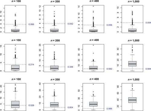
Table 3. Proportion of replicates that the Yule-Simon distribution is rejected at nominal level 0.05.

	n = 100	n = 200	n = 400	n = 1000
$\text{β}=1$	0.066	0.042	0.056	0.054
$\text{β}=1.5$	0.214	0.348	0.582	0.944
$\text{β}=2$	0.528	0.804	0.986	1.000

4. Real data application

Seal (1947, 1952) provided data on insurance shares for 12 different age periods. The original data is about male lives assured in a British life office, maintained for administrative purposes. The analysed data is a random subset, and every tenth names in this list were included until the total of 2000 was reached. The lives sampled are scheduled according to the year of birth and the number of policies in force. The group is represented by the central age.

Seal (1952) fitted the data using the discrete Pareto, with probability mass function $P(X=k)=k^{-d}/\zeta \left(d\right),k=1,2,3,\dots ,d>1,$where $\zeta \left(d\right)$ is a normalization constant, and the parameter d is estimated by the MLE. Here we apply the Waring distribution to fit the data. For the age periods centred at 17.5 and 22.5, the maximal number of shares is 2. The EFF method leads to negative parameter estimates, while the MLE is proved not to exist as in Remark 2.1. We focus on the rest 10 groups, with central ages from 27.5 to 72.5. Among these 10 groups, for the group with central age 67.5, we have n = 45 and $n_1=33,n_2=7,n_3=4,n_4=1$, and it is easy to verify that (9(9) $\{p_2+2p_3+\cdots +(m-1)p_m{\}}^2<p_3+3p_4+\cdots +\frac{(m-1)(m-2)}{2}{p}_m.$(9) ) does not hold. Thus the MLE does not exist. If we directly apply the optimization algorithm, we get $\hat{\alpha }=1,687,133.2,\widehat{\text{β}}=675,078.4$, which is meaningless. However, if we use the EFF method, we get $\hat{\alpha }=11,\widehat{\text{β}}=4$, and the resulted fitting is reasonably good. Thus, we need to be careful in using the MLE. Table 4 summarizes the comparison of the actual distribution with discrete Pareto law fitting, Waring fitting with EFF and MLE, we find that the Waring distribution fits the data slightly better than the discrete Pareto law.

Table 4. Comparison of actual distribution (A) with discrete Pareto law fitting (P), Waring fitting with EFF (E) and MLE (M).

Central age	27.5				32.5				37.5				42.5				47.5
j	P	E	M	A	P	E	M	A	P	E	M	A	P	E	M	A	P	E	M	A
1	101.9	101	100.8	101	242.7	241	241.2	241	285.3	283	283.8	283	305.2	307	306.6	307	235.9	233	233.6	233
2	6.8	8.5	8.7	8	22.3	24.6	24.4	26	28.6	30.9	30.3	35	35.5	33.8	33.4	31	28.8	31.9	31.4	35
3	1.4	1.2	1.2	2	5.5	5.8	5.8	3	7.5	8	7.9	4	10.1	10	10.1	12	8.4	9.2	9.1	4
4	0.5	0.2	0.2	0	2	1.9	2	3	2.9	2.9	2.9	2	4.1	4.2	4.3	6	3.5	3.6	3.6	5
5	0.2	0.1	0	0	0.9	0.8	0.8	0	1.4	1.3	1.3	0	2.1	2.1	2.2	0	1.8	1.7	1.7	3
6	0.1	0	0	0	0.5	0.4	0.4	2	0.8	0.7	0.7	2	1.2	1.2	1.3	1	1	0.9	0.9	0
7	0.1	0	0	0	0.3	0.2	0.2	0	0.4	0.4	0.4	0	0.7	0.7	0.8	2	0.6	0.5	0.5	1
8	0	0	0	0	0.2	0.1	0.1	0	0.3	0.2	0.2	1	0.5	0.5	0.5	0	0.4	0.3	0.3	0
9	0	0	0	0	0.1	0.1	0.1	0	0.2	0.1	0.1	1	0.3	0.3	0.4	0	0.3	0.2	0.2	0
10	0	0	0	0	0.1	0	0	0	0.1	0.1	0.1	0	0.2	0.2	0.3	0	0.2	0.1	0.1	0
11	0	0	0	0	0.1	0	0	0	0.1	0.1	0.1	0	0.2	0.2	0.2	2	0.2	0.1	0.1	0
12	0	0	0	0	0	0	0	0	0.1	0	0	0	0.1	0.1	0.2	0	0.1	0.1	0.1	0
13	0	0	0	0	0	0	0	0	0.1	0	0	0	0.1	0.1	0.1	0	0.1	0.1	0.1	1
14	0	0	0	0	0	0	0	0	0	0	0	0	0.1	0.1	0.1	0	0.1	0	0	0
15	0	0	0	0	0	0	0	0	0	0	0	0	0.1	0.1	0.1	0	0.1	0	0	0
16	0	0	0	0	0	0	0	0	0	0	0	0	0.1	0.1	0.1	0	0.1	0	0	0
17	0	0	0	0	0	0	0	0	0	0	0	0	0	0	0.1	0	0	0	0	0
18	0	0	0	0	0	0	0	0	0	0	0	0	0	0	0.1	0	0	0	0	0
Totals	111	111	110.9	111	274.7	274.9	275	275	327.8	327.7	327.8	328	360.6	360.7	360.9	361	281.6	281.7	281.7	282
Central age	52.5				57.5				62.5				67.5				72.5
j	P	E	M	A	P	E	M	A	P	E	M	A	P	E	M	A	P	E	M	A
1	199.3	200	200	200	110.8	108	107.7	108	72	69	69.5	69	35.1	33	/	33	27.4	26	24.9	26
2	24.7	24.1	23.6	24	16.6	20.1	20.1	20	6.3	7.1	7.1	10	5.5	8.3	/	7	5.2	6.9	7.7	5
3	7.3	7.3	7.3	7	5.5	6.3	6.4	5	1.5	2.2	2.1	1	1.9	2.4	/	4	2	2.5	2.9	4
4	3	3.1	3.2	2	2.5	2.6	2.6	2	0.6	1	0.9	0	0.9	0.8	/	1	1	1.1	1.2	1
5	1.6	1.6	1.6	0	1.4	1.2	1.3	4	0.3	0.5	0.5	0	0.5	0.3	/	0	0.6	0.6	0.6	2
6	0.9	0.9	1	3	0.8	0.7	0.7	0	0.1	0.3	0.3	0	0.3	0.1	/	0	0.4	0.3	0.3	0
7	0.6	0.6	0.6	1	0.5	0.4	0.4	0	0.1	0.2	0.2	0	0.2	0.1	/	0	0.3	0.2	0.2	0
8	0.4	0.4	0.4	1	0.4	0.2	0.2	1	0	0.1	0.1	0	0.1	0	/	0	0.2	0.1	0.1	0
9	0.3	0.3	0.3	0	0.3	0.2	0.2	0	0	0.1	0.1	0	0.1	0	/	0	0.1	0.1	0.1	0
10	0.2	0.2	0.2	1	0.2	0.1	0.1	0	0	0.1	0.1	0	0.1	0	/	0	0.1	0	0	0
11	0.1	0.1	0.2	0	0.2	0.1	0.1	0	0	0.1	0	0	0.1	0	/	0	0.1	0	0	0
12	0.1	0.1	0.1	0	0.1	0.1	0.1	0	0	0	0	0	0	0	/	0	0.1	0	0	0
13	0.1	0.1	0.1	0	0.1	0	0	0	0	0	0	0	0	0	/	0	0.1	0	0	0
14	0.1	0.1	0.1	0	0.1	0	0	0	0	0	0	0	0	0	/	0	0	0	0	0
15	0.1	0	0.1	0	0.1	0	0	0	0	0	0	0	0	0	/	0	0	0	0	0
16	0	0	0	0	0.1	0	0	0	0	0	0	0	0	0	/	0	0	0	0	0
17	0	0	0	0	0	0	0	0	0	0	0	0	0	0	/	0	0	0	0	0
18	0	0	0	0	0	0	0	0	0	0	0	1	0	0	/	0	0	0	0	0
Totals	238.8	238.9	238.8	239	139.7	140	139.9	140	80.9	80.7	80.9	81	44.8	45	/	45	37.6	37.8	38	38

5. Discussion

To fit a given data set by the Waring distribution, we need to verify the existence condition of the MLE of the Waring parameters before we use the MLE. If the existence condition is not satisfied, it means that the likelihood is maximized at the boundary, i.e., infinity. Therefore, if we directly apply the optimization algorithm to the likelihood function, the MLE may be far from the true parameters; see for example, we get MLE $\hat{\alpha }=1,687,133.2,\widehat{\text{β}}=675,078.4$ for the group with central age 67.5, where in fact that the MLE does not exist. In such cases, we can use the EFF method if the EFF estimates are in reasonable scales. Based on the simulation studies and the real data analysis, we find that, when the sample size is small or the maximum observed value is small, the MLE is less likely to exist, and when the sample size is big and the maximum observed value is large, the MLE is more likely to exist. Nevertheless, we need verify the existence condition for the MLE.

Acknowledgements

The authors would like to thank two anonymous reviewers, an associate editor and the editor for constructive comments and helpful suggestions.

Disclosure statement

No potential conflict of interest was reported by the author(s).

Additional information

Funding

This work is partially supported by National Natural Science Foundation of China [Grant Numbers 11671096, 11690013, 11731011, 11871376] and Natural Science Foundation of Shanghai [Grant Number 21ZR1420700].

Appendices

The appendix contains some useful lemmas and technical proofs.

Appendix 1. Some useful lemmas

Lemma A.1

Define $g\left(x\right)=\frac{1}{\frac{1}{a_{1}x+b_1}+\cdots +\frac{1}{a_{k}x+b_k}},x>0,$where $a_1,\dots ,a_k$ are positive and $b_1,\dots ,b_k$ are nonnegative. Then $g\left(x\right)$ is an increasing and concave function.

Proof.

It is easy to derive that $\begin{array}{rl}{g}^{\mathrm{\prime }}\left(x\right)& =g^2\left(x\right)\{\frac{a_1}{(a_{1}x+b_1{)}^2}+\cdots +\frac{a_k}{(a_{k}x+b_k{)}^2}\}>0,\\ g^{\mathrm{\prime }\mathrm{\prime }}\left(x\right)& =2g^3\left(x\right)[{\{\frac{a_1}{(a_{1}x+b_1{)}^2}+\cdots +\frac{a_k}{(a_{k}x+b_k{)}^2}\}}^2\\ & -(\frac{1}{a_{1}x+b_1}+\cdots +\frac{1}{a_{k}x+b_k})\{\frac{a_1^2}{(a_{1}x+b_1{)}^3}+\cdots +\frac{a_k^2}{(a_{k}x+b_k{)}^3}\}]\\ & =-\sum _{1\le i<j\le k}\frac{1}{(a_{i}x+b_i)(a_{j}x+b_j)}{(\frac{1}{a_{i}x+b_i}-\frac{1}{a_{j}x+b_j})}^2<0.\text{■}\end{array}$

Lemma A.2

When $x\to \mathrm{\infty }$, we have $\begin{array}{rl}& \frac{x^m+a_1{x}^{m-1}+a_2{x}^{m-2}+\cdots }{b_1{x}^{m-1}+b_2{x}^{m-2}+b_3{x}^{m-3}+\cdots }\\ & =\frac{1}{b_1}x+\frac{a_1{b}_1-b_2}{b_1^2}+\frac{a_2{b}_1^2-b_1{b}_3-a_1{b}_1{b}_2+b_2^2}{b_1^3}\cdot \frac{1}{x}+O\left(\frac{1}{x^2}\right).\end{array}$

Proof.

Assume that $\frac{x^m+a_1{x}^{m-1}+a_2{x}^{m-2}+\cdots }{b_1{x}^{m-1}+b_2{x}^{m-2}+b_3{x}^{m-3}+\cdots }=\frac{1}{b_1}x+c+d\cdot \frac{1}{x}+O\left(\frac{1}{x^2}\right).$Then $\begin{array}{rl}& x^m+a_1{x}^{m-1}+a_2{x}^{m-2}+\cdots \\ & =(b_1{x}^{m-1}+b_2{x}^{m-2}+b_3{x}^{m-3}+\cdots )\cdot (\frac{1}{b_1}x+c+d\cdot \frac{1}{x}+\cdots )\\ & =x^m+(b_{1}c+\frac{b_2}{b_1})x^{m-1}+(b_{1}d+b_{2}c+\frac{b_3}{b_1})x^{m-2}+\cdots ,\end{array}$which indicates that: (i) $b_{1}c+b_2/b_1=a_1$, and then $c=\frac{a_1{b}_1-b_2}{b_1^2}$; (ii) $b_{1}d+b_{2}c+\frac{b_3}{b_1}=a_2$, and then $d=\frac{a_2{b}_1^2-b_1{b}_3-a_1{b}_1{b}_2+b_2^2}{b_1^3}$. The proof is completed.

Appendix 2. Technical Proofs

Appendix 2.1. Proof of Lemmas 2.3–2.4

Proof

Proof of Lemma 2.3

Since for any β, ${\ell }_n\left(\alpha \right(\text{β}),\text{β})=\underset{\alpha }{max}{\ell }_n(\alpha ,\text{β})$. Thus, to prove ${\ell }_n\left(\alpha \right({\text{β}}_1),{\text{β}}_1)=\underset{\alpha ,\text{β}}{max}{\ell }_n(\alpha ,\text{β})$, we only need prove that ${\text{β}}_1$ maximizes ${\ell }_n\left(\alpha \right(\text{β}),\text{β})$. Therefore, we only need prove that $\mathrm{\partial }{\ell }_n\left(\alpha \right(\text{β}),\text{β})/\mathrm{\partial }\text{β}{|}_{\text{β}={\text{β}}_1}=0$, $\mathrm{\partial }{\ell }_n\left(\alpha \right(\text{β}),\text{β})/\mathrm{\partial }\text{β}>0$ for $\text{β}<{\text{β}}_1$ and $\mathrm{\partial }{\ell }_n\left(\alpha \right(\text{β}),\text{β})/\mathrm{\partial }\text{β}<0$ for $\text{β}>{\text{β}}_1$.

Consider the following decomposition, $\begin{array}{rl}& \frac{{\ell }_n\left(\alpha \right(\text{β}+\mathrm{\Delta }\text{β}),\text{β}+\mathrm{\Delta }\text{β})-{\ell }_n\left(\alpha \right(\text{β}),\text{β})}{\mathrm{\Delta }\text{β}}\\ & =\frac{{\ell }_n\left(\alpha \right(\text{β}+\mathrm{\Delta }\text{β}),\text{β}+\mathrm{\Delta }\text{β})-{\ell }_n\left(\alpha \right(\text{β}),\text{β}+\mathrm{\Delta }\text{β})}{\mathrm{\Delta }\text{β}}+\frac{{\ell }_n\left(\alpha \right(\text{β}),\text{β}+\mathrm{\Delta }\text{β})-{\ell }_n\left(\alpha \right(\text{β}),\text{β})}{\mathrm{\Delta }\text{β}}\\ & \to {\{\frac{\mathrm{\partial }{\ell }_n(\alpha ,\text{β})}{\mathrm{\partial }\alpha }\cdot \frac{\mathrm{\partial }\alpha \left(\text{β}\right)}{\mathrm{\partial }\text{β}}+\frac{\mathrm{\partial }\ell (\alpha ,\text{β})}{\mathrm{\partial }\text{β}}\}|}_{\alpha =\alpha \left(\text{β}\right)},\end{array}$where $\frac{\mathrm{\partial }{\ell }_n(\alpha ,\text{β})}{\mathrm{\partial }\alpha }{|}_{\alpha =\alpha \left(\text{β}\right)}=0$, and thus $\frac{\mathrm{\partial }\ell (\alpha ,\text{β})}{\mathrm{\partial }\text{β}}{|}_{\alpha =\alpha \left(\text{β}\right)}$ totally determines the sign of $\frac{\mathrm{\partial }\ell \left(\alpha \right(\text{β}),\text{β})}{\mathrm{\partial }\text{β}}$. The proof is completed.

Proof

Proof of Lemma 2.4

We use the method of contradiction. If the conclusion is not correct, then there exists $x_1>a$ such that $t_1\left(x_1\right)=t_2\left(x_1\right)$, $t_1\left(x\right)>t_2\left(x\right)$ for $x<x_1$ and $t_1\left(x\right)<t_2\left(x\right)$ for $x\in (x_1,x_1+{\delta }_0)$ for some ${\delta }_0>0$. By assumption (D), the curves $y=t_1\left(x\right)$ and $y=t_2\left(x\right)$ will intersect again after $(x_1,t_1(x_1\left)\right)$, i.e., there exists $x_2>x_1$ such that $t_1\left(x_2\right)=t_2\left(x_2\right)$, $t_1\left(x\right)<t_2\left(x\right)$ for $x\in (x_1,x_2)$ and $t_1\left(x\right)>t_2\left(x\right)$ for $x>x_2$ (suppose that there exists only one such $x_2$, otherwise, we consider the largest intersection). According to assumption (D), take one point $x_{\ast }\in ({\delta }_4^{\ast },\mathrm{\infty })$ (which is of course greater than $x_2$), use $(x_2,t(x_2\left)\right)$ as the starting point, and then take a ray interpolating $(x_{\ast },t_1(x_{\ast }\left)\right)$. Let $x_{\ast }$ diverge to infinity so that the point $(x_{\ast },t_1(x_{\ast }\left)\right)$ moves along the curve $y=t_1\left(x\right)$. Since $t_1\left(x\right)$ is increasing and concave, the ray interpolating $(x_{\ast },t_1(x_{\ast }\left)\right)$ tilts down around the start point $(x_2,t(x_2\left)\right)$. By assumption (C), when $x_{\ast }\to \mathrm{\infty }$, the slope of the ray $\frac{t_1\left(x_{\ast }\right)-t_1\left(x_2\right)}{x_{\ast }-x_2}\to c^{\ast }.$Thus the limit of the ray is a ray with start point $(x_2,t_1(x_2\left)\right)$ and slope $c^{\ast }$, denoted as L, and the curve $y=t_1\left(x\right)$ is above L.

Note that the start point of the ray L, $(x_2,t(x_2\left)\right)$, is on the curve $y=t_2\left(x\right)$. By assumption (D), there exists an $x^{\ast }$, which satisfies that, the curve $y=t_2\left(x\right)$ intersects L at $(x^{\ast },t_2(x^{\ast }\left)\right)$ and $y=t_2\left(x\right)$ lies below L for $x\in (x^{\ast },x^{\ast }+{\delta }_5^{\ast })$ with some positive ${\delta }_5^{\ast }$. Without loss of generality, we assume that $x_2$ is such point, that is, $y=t_2\left(x\right)$ lies below L for $x\in (x_2,x_2+{\delta }_5^{\ast })$.

Through the intersection $(x_2,t_1(x_2\left)\right)$, we make tangent line of the curve $y=t_2\left(x\right)$. If the tangent line coincides with the ray, then take another point $x^{\ast \ast }\in (x_2,x_2+{\delta }_5^{\ast })$, and make another tangent line of the curve $y=t_2\left(x\right)$ through the point $(x^{\ast \ast },t_2(x^{\ast \ast }\left)\right)$. Since $y=t_2\left(x\right)$ is increasing and concave, if the tangent line (of $y=t_2\left(x\right)$) through $(x_2,t_1(x_2\left)\right)$ coincides with the ray L, the tangent line through $(x^{\ast \ast },t_2(x^{\ast \ast }\left)\right)$ does not coincide with L. Note that the curve $y=t_1\left(x\right)$ is above L, while $y=t_2\left(x\right)$ is below the tangent line (a concave curve is always below its tangent line) which is below the ray L (the one which does not coincide with L must be below L according to the above discussion). Therefore, $\underset{x\to \mathrm{\infty }}{lim}\frac{t_1\left(x\right)}{x}\ne \underset{x\to \mathrm{\infty }}{lim}\frac{t_2\left(x\right)}{x}$, which contradicts with assumption (C).

To summary, no such $x_1>a$ exists that $t_1\left(x_1\right)=t_2\left(x_1\right)$, $t_1\left(x\right)>t_2\left(x\right)$ for $x<x_1$ and $t_1\left(x\right)<t_2\left(x\right)$ for $x\in (x_1,x_1+{\delta }_0)$ for some ${\delta }_0>0$. We conclude that, $t_1\left(x\right)\ge t_2\left(x\right)$ for $x\in (a,\mathrm{\infty })$. The proof of Lemma 2.4 is completed.

Appendix 2.2. Proof of Propositions 2.1–2.2

Proof

Proof of Propositions 2.1

Proof of Property 1. If $\text{β}\to 0$, we have $g_1(\alpha ,\text{β})\to \frac{1}{\frac{1}{\alpha }+\frac{\sum _{s=2}^m{p}_s}{\alpha +1}+\frac{\sum _{s=3}^m{p}_s}{\alpha +2}+\cdots +\frac{p_m}{\alpha +m-1}}\to 0,$when $\alpha \to 0$. Therefore, when $\text{β}\to 0$, the intersection of $y=g_1(\alpha ,\text{β})$ and $y=\alpha$ converges to the origin of coordinates.

Proof of Property 2. If $\text{β}\to \mathrm{\infty }$, then for any $\alpha >0$, we have $g_1(\alpha ,\text{β})\to \mathrm{\infty }$. Thus, if $\text{β}\to \mathrm{\infty }$, then $\alpha \left(\text{β}\right)\to \mathrm{\infty }$ because $\left(\alpha \right(\text{β}),\text{β})$ is the intersection. We have $\begin{array}{rl}\alpha \left(\text{β}\right)& =\frac{1}{\frac{1}{\alpha \left(\text{β}\right)+\text{β}}+\frac{\sum _{s=2}^m{p}_s}{\alpha \left(\text{β}\right)+\text{β}+1}+\frac{\sum _{s=3}^m{p}_s}{\alpha \left(\text{β}\right)+\text{β}+2}+\cdots +\frac{p_m}{\alpha \left(\text{β}\right)+\text{β}+m-1}}\\ & =\frac{\left\{\alpha \right(\text{β})+\text{β}{\}}^m+a_1\cdot \{\alpha \left(\text{β}\right)+\text{β}{\}}^{m-1}+a_2\cdot \left\{\alpha \right(\text{β})+\text{β}{\}}^{m-2}+\cdots }{b_1\cdot \left\{\alpha \right(\text{β})+\text{β}{\}}^{m-1}+b_2\cdot \{\alpha \left(\text{β}\right)+\text{β}{\}}^{m-2}+b_3\cdot \left\{\alpha \right(\text{β})+\text{β}{\}}^{m-3}+\cdots },\end{array}$where $\begin{array}{rl}{a}_1& =\frac{m(m-1)}{2},a_2=\frac{1}{24}m(m-1)(m-2)(3m-1),b_1=1+{\eta }_1,\\ b_2& =\frac{m(m-1)}{2}(1+{\eta }_1)+{\eta }_1-{\eta }_2,\\ b_3& =\frac{m(m-1)(m-2)(3m-1)}{24}+\frac{m(m-1)(3m^2-7m+14)+24}{24}{\eta }_1\\ & -\{\frac{m(m-1)}{2}+2\}{\eta }_2+{\eta }_3.\end{array}$Based on Lemma A.2, tedious calculation yields $\alpha \left(\text{β}\right)=\frac{1}{1+{\eta }_1}\left\{\alpha \right(\text{β})+\text{β}\}+c_{\alpha }^{\mathrm{\prime }}+\frac{d_{\alpha }}{\alpha \left(\text{β}\right)+\text{β}}+\cdots ,$where $c_{\alpha }^{\mathrm{\prime }}=\frac{{\eta }_2-{\eta }_1}{(1+{\eta }_1{)}^2},d_{\alpha }=\frac{{\eta }_2^2-{\eta }_1{\eta }_3-{\eta }_1+2{\eta }_2-{\eta }_3}{(1+{\eta }_1{)}^3}.$Simple algebra yields $\alpha \left(\text{β}\right)=\frac{1}{{\eta }_1}\text{β}+\frac{c_{\alpha }^{\mathrm{\prime }}(1+{\eta }_1)}{{\eta }_1}+\frac{1+{\eta }_1}{{\eta }_1}\frac{d_{\alpha }}{\alpha \left(\text{β}\right)+\text{β}}+\cdots =\frac{1}{{\eta }_1}\text{β}+c_{\alpha }+\frac{d_{\alpha }}{\text{β}}+O\left(1/{\text{β}}^2\right),$where $c_{\alpha }=\frac{c_{\alpha }^{\mathrm{\prime }}(1+{\eta }_1)}{{\eta }_1}=\frac{{\eta }_2-{\eta }_1}{{\eta }_1(1+{\eta }_1)}$.

Proof of Property 3. Since (A1) $\frac{1}{\alpha \left(\text{β}\right)}=\frac{1}{\alpha \left(\text{β}\right)+\text{β}}+\frac{\sum _{s=2}^m{p}_s}{\alpha \left(\text{β}\right)+\text{β}+1}+\cdots +\frac{p_m}{\alpha \left(\text{β}\right)+\text{β}+m-1},$(A1) taking derivative with respect to β on both sides of (A1(A1) $\frac{1}{\alpha \left(\text{β}\right)}=\frac{1}{\alpha \left(\text{β}\right)+\text{β}}+\frac{\sum _{s=2}^m{p}_s}{\alpha \left(\text{β}\right)+\text{β}+1}+\cdots +\frac{p_m}{\alpha \left(\text{β}\right)+\text{β}+m-1},$(A1) ), we have ${\alpha }^{\mathrm{\prime }}\left(\text{β}\right)={\alpha }^2\left(\text{β}\right)[\frac{{\alpha }^{\mathrm{\prime }}\left(\text{β}\right)+1}{\left\{\alpha \right(\text{β})+\text{β}{\}}^2}+\frac{\left\{{\alpha }^{\mathrm{\prime }}\right(\text{β})+1\}\sum _{s=2}^m{p}_s}{\left\{\alpha \right(\text{β})+\text{β}+1{\}}^2}+\cdots +\frac{\left\{{\alpha }^{\mathrm{\prime }}\right(\text{β})+1\}{p}_m}{\left\{\alpha \right(\text{β})+\text{β}+m-1{\}}^2}].$Simple algebra leads to ${\alpha }^{\mathrm{\prime }}\left(\text{β}\right)=\frac{u\left(\text{β}\right)}{1-u\left(\text{β}\right)},$where (A2) $u\left(\text{β}\right)=\frac{\frac{1}{\left\{\alpha \right(\text{β})+\text{β}{\}}^2}+\frac{\sum _{s=2}^m{p}_s}{\left\{\alpha \right(\text{β})+\text{β}+1{\}}^2}+\cdots +\frac{p_m}{\left\{\alpha \right(\text{β})+\text{β}+m-1{\}}^2}}{{\{\frac{1}{\alpha \left(\text{β}\right)+\text{β}}+\frac{\sum _{s=2}^m{p}_s}{\alpha \left(\text{β}\right)+\text{β}+1}+\cdots +\frac{p_m}{\alpha \left(\text{β}\right)+\text{β}+m-1}\}}^2}>0.$(A2) Furthermore, since $\begin{array}{rl}& {\{\frac{1}{\alpha \left(\text{β}\right)+\text{β}}+\frac{\sum _{s=2}^m{p}_s}{\alpha \left(\text{β}\right)+\text{β}+1}+\cdots +\frac{p_m}{\alpha \left(\text{β}\right)+\text{β}+m-1}\}}^2\\ & =\sum _{i=1}^m\left[\frac{\sum _{s=i}{p}_s}{\alpha \left(\text{β}\right)+\text{β}+i-1}\left\{\sum _{j=1}^m\frac{\sum _{s=j}^m{p}_s}{\alpha \left(\text{β}\right)+\text{β}+j-1}\right\}\right]\\ & >\sum _{i=1}^m\left\{\frac{\sum _{s=i}{p}_s}{\alpha \left(\text{β}\right)+\text{β}+i-1}\frac{1}{\alpha \left(\text{β}\right)+\text{β}}\right\}>\sum _{i=1}^m\frac{\sum _{s=i}{p}_s}{\left\{\alpha \right(\text{β})+\text{β}+i-1{\}}^2},\end{array}$which indicates that $u\left(\text{β}\right)<1$. Therefore, ${\alpha }^{\mathrm{\prime }}\left(\text{β}\right)>0$.

Taking derivative with respect to β twice on both sides of (A1(A1) $\frac{1}{\alpha \left(\text{β}\right)}=\frac{1}{\alpha \left(\text{β}\right)+\text{β}}+\frac{\sum _{s=2}^m{p}_s}{\alpha \left(\text{β}\right)+\text{β}+1}+\cdots +\frac{p_m}{\alpha \left(\text{β}\right)+\text{β}+m-1},$(A1) ), we have $\begin{array}{rl}& {\alpha }^{\mathrm{\prime }\mathrm{\prime }}\left(\text{β}\right)\\ & =2{\alpha }^3\left(\text{β}\right)({[\frac{{\alpha }^{\mathrm{\prime }}\left(\text{β}\right)+1}{\left\{\alpha \right(\text{β})+\text{β}{\}}^2}+\frac{\left\{{\alpha }^{\mathrm{\prime }}\right(\text{β})+1\}\sum _{s=2}^m{p}_s}{\left\{\alpha \right(\text{β})+\text{β}+1{\}}^2}+\cdots +\frac{\left\{{\alpha }^{\mathrm{\prime }}\right(\text{β})+1\}{p}_m}{\left\{\alpha \right(\text{β})+\text{β}+m-1{\}}^2}]}^2\\ & -\{\frac{1}{\alpha \left(\text{β}\right)+\text{β}}+\frac{\sum _{s=2}^m{p}_s}{\alpha \left(\text{β}\right)+\text{β}+1}+\frac{\sum _{s=3}^m{p}_s}{\alpha \left(\text{β}\right)+\text{β}+2}+\cdots +\frac{p_m}{\alpha \left(\text{β}\right)+\text{β}+m-1}\}\\ & \times [\frac{\left\{{\alpha }^{\mathrm{\prime }}\right(\text{β})+1{\}}^2}{\left\{\alpha \right(\text{β})+\text{β}{\}}^3}+\frac{\left\{{\alpha }^{\mathrm{\prime }}\right(\text{β})+1{\}}^2\sum _{s=2}^m{p}_s}{\left\{\alpha \right(\text{β})+\text{β}+1{\}}^3}+\cdots +\frac{\left\{{\alpha }^{\mathrm{\prime }}\right(\text{β})+1{\}}^2{p}_m}{\left\{\alpha \right(\text{β})+\text{β}+m-1{\}}^3}])\\ & =-2{\alpha }^3\left(\text{β}\right)\left\{{\alpha }^{\mathrm{\prime }}\right(\text{β})+1{\}}^2\\ & \times \left[\sum _{0\le i<j\le m-1}\frac{\sum _{s=i+1}^m{p}_s\sum _{s=j+1}^m{p}_s}{\left\{\alpha \right(\text{β})+\text{β}+i\}\left\{\alpha \right(\text{β})+\text{β}+j\}}{\{\frac{1}{\alpha \left(\text{β}\right)+\text{β}+i}-\frac{1}{\alpha \left(\text{β}\right)+\text{β}+j}\}}^2\right]\\ & <0.\end{array}$

Proof of Property 4. If $\text{β}\to 0$, then $\alpha \left(\text{β}\right)\to 0$, and thus (A2(A2) $u\left(\text{β}\right)=\frac{\frac{1}{\left\{\alpha \right(\text{β})+\text{β}{\}}^2}+\frac{\sum _{s=2}^m{p}_s}{\left\{\alpha \right(\text{β})+\text{β}+1{\}}^2}+\cdots +\frac{p_m}{\left\{\alpha \right(\text{β})+\text{β}+m-1{\}}^2}}{{\{\frac{1}{\alpha \left(\text{β}\right)+\text{β}}+\frac{\sum _{s=2}^m{p}_s}{\alpha \left(\text{β}\right)+\text{β}+1}+\cdots +\frac{p_m}{\alpha \left(\text{β}\right)+\text{β}+m-1}\}}^2}>0.$(A2) ) indicates that $u\left(\text{β}\right)\to 1$; therefore ${\alpha }^{\mathrm{\prime }}\left(\text{β}\right)\to \mathrm{\infty }$. If $\text{β}\to \mathrm{\infty }$, then $\alpha \left(\text{β}\right)\to \mathrm{\infty }$, and thus (A2(A2) $u\left(\text{β}\right)=\frac{\frac{1}{\left\{\alpha \right(\text{β})+\text{β}{\}}^2}+\frac{\sum _{s=2}^m{p}_s}{\left\{\alpha \right(\text{β})+\text{β}+1{\}}^2}+\cdots +\frac{p_m}{\left\{\alpha \right(\text{β})+\text{β}+m-1{\}}^2}}{{\{\frac{1}{\alpha \left(\text{β}\right)+\text{β}}+\frac{\sum _{s=2}^m{p}_s}{\alpha \left(\text{β}\right)+\text{β}+1}+\cdots +\frac{p_m}{\alpha \left(\text{β}\right)+\text{β}+m-1}\}}^2}>0.$(A2) ) indicates that $u\left(\text{β}\right)\to \frac{1}{1+\sum _{t=2}^m\sum _{s=t}^m{p}_s}$; therefore ${\alpha }^{\mathrm{\prime }}\left(\text{β}\right)\to \frac{1}{\sum _{t=2}^m\sum _{s=t}^m{p}_s}$.

Proof of Property 5. According to (3(3) $\begin{array}{rl}& \frac{1}{n}\cdot \frac{\mathrm{\partial }{\ell }_n(\alpha ,\text{β})}{\mathrm{\partial }\alpha }\\ & =\frac{1}{\alpha }-(\frac{1}{\alpha +\text{β}}+\frac{\sum _{s=2}^m{p}_s}{\alpha +\text{β}+1}+\frac{\sum _{s=3}^m{p}_s}{\alpha +\text{β}+2}+\cdots +\frac{p_m}{\alpha +\text{β}+m-1})=0,\end{array}$(3) ), the conditional maximum likelihood equation of α can be rewritten as $\frac{\alpha }{\alpha +\text{β}}+\frac{\alpha \sum _{s=2}^m{p}_s}{\alpha +\text{β}+1}+\frac{\alpha \sum _{s=3}^m{p}_s}{\alpha +\text{β}+2}+\cdots +\frac{\alpha p_m}{\alpha +\text{β}+m-1}=1.$Let $f\left(\alpha \right)=\frac{\alpha }{\alpha +\text{β}}+\frac{\alpha \sum _{s=2}^m{p}_s}{\alpha +\text{β}+1}+\frac{\alpha \sum _{s=3}^m{p}_s}{\alpha +\text{β}+2}+\cdots +\frac{\alpha p_m}{\alpha +\text{β}+m-1},$and then $f\left(\alpha \right)$ is an increasing function of α. Since $f\left(\alpha \right(\text{β}\left)\right)=1$, then x is less than, equal to or greater than $\alpha \left(\text{β}\right)$ which is equivalent to that $f\left(x\right)$ is less than, equal to or greater than 1. Therefore, $\alpha \left(\text{β}\right)=Z\left(\text{β}\right)$ is equivalent to $f\left(Z\right(\text{β}\left)\right)=1$. Since $Z\left(\text{β}\right)$ is a polynomial or fractional function of β, then $f\left(Z\right(\text{β}\left)\right)=\frac{Z\left(\text{β}\right)}{Z\left(\text{β}\right)+\text{β}}+\frac{Z\left(\text{β}\right)\sum _{s=2}^m{p}_s}{Z\left(\text{β}\right)+\text{β}+1}+\frac{Z\left(\text{β}\right)\sum _{s=3}^m{p}_s}{Z\left(\text{β}\right)+\text{β}+2}+\cdots +\frac{Z\left(\text{β}\right)p_m}{Z\left(\text{β}\right)+\text{β}+m-1}=1$is a high-ordered polynomial equation, which has finite number of solutions.

Proof

Proof of Proposition 2.2

The proofs of Properties 1* and 5* are similar to the proofs of Properties 1 and 5 in Proposition 2.1, respectively, and Property 3* follows from Lemma A.1. In the following, we present the proofs of Properties 2* and 4*.

Proof of Property 2*. By Lemma A.2, it is easy to obtain $h\left(\text{β}\right)=\frac{{\text{β}}^{m-1}+a_1{\text{β}}^{m-2}+a_2{\text{β}}^{m-3}+\cdots }{b_1{\text{β}}^{m-2}+b_2{\text{β}}^{m-3}+b_3{\text{β}}^{m-4}+\cdots },$where $\begin{array}{rl}{a}_1& =\frac{(m-1)(m-2)}{2},a_2=\frac{(m-1)(m-2)(m-3)(3m-4)}{24},b_1={\eta }_1,\\ b_2& =\frac{(m-2)(m-1)+4}{2}{\eta }_1-{\eta }_2,\\ b_3& =\frac{(m-2)(m-1)(3m^2-13m+36)+96}{24}{\eta }_1-\frac{m^2-3m+10}{2}{\eta }_2+{\eta }_3.\end{array}$Therefore, we have $h\left(\text{β}\right)=\frac{1}{{\eta }_1}\text{β}+c_h+d_h\frac{1}{\text{β}}+O\left(1/{\text{β}}^2\right),$where $\begin{array}{rl}{c}_h& =\frac{a_1{b}_1-b_2}{b_1^2}=\frac{{\eta }_2-2{\eta }_1}{{\eta }_1^2},\\ d_h& =\frac{a_2{b}_1^2-b_1{b}_3-a_1{b}_1{b}_2+b_2^2}{b_1^3}=\frac{{\eta }_2^2-{\eta }_1{\eta }_3}{{\eta }_1^3}.\end{array}$Proof of Property 4*. It is easy to derive that $\begin{array}{rl}{h}^{\mathrm{\prime }}\left(\text{β}\right)& =\frac{\frac{\sum _{s=2}{p}_s}{{\text{β}}^2}+\frac{\sum _{s=3}{p}_s}{(\text{β}+1{)}^2}+\cdots +\frac{p_m}{(\text{β}+m-2{)}^2}}{(\frac{\sum _{s=2}{p}_s}{\text{β}}+\frac{\sum _{s=3}{p}_s}{\text{β}+1}+\cdots +\frac{p_m}{\text{β}+m-2})}\\ & =\frac{\left(\sum _{t=2}^m\sum _{s=t}^m{p}_s\right){\text{β}}^{2(m-1)}+\cdots +\left(\sum _{s=2}^m{p}_s\right)\left\{\right(m-2)!{\}}^2}{(\sum _{t=2}^m\sum _{s=t}^m{p}_s{)}^2{\text{β}}^{2(m-1)}+\cdots +(\sum _{s=2}^m{p}_s{)}^2\left\{\right(m-2)!{\}}^2},\end{array}$and we have $\begin{array}{rl}{h}^{\mathrm{\prime }}\left(\text{β}\right)& \to \frac{\left(\sum _{s=2}^m{p}_s\right)\left\{\right(m-2)!{\}}^2}{\left(\sum _{s=2}^m{p}_s{)}^2\right\{(m-2)!{\}}^2}=\frac{1}{\sum _{s=2}^m{p}_s},\mathrm{w}\mathrm{h}\mathrm{e}\mathrm{n}\text{β}\to 0,\\ h^{\mathrm{\prime }}\left(\text{β}\right)& \to \frac{\sum _{t=2}^m\sum _{s=t}^m{p}_s}{(\sum _{t=2}^m\sum _{s=t}^m{p}_s{)}^2}=\frac{1}{\sum _{t=2}^m\sum _{s=t}^m{p}_s}=\frac{1}{{\eta }_1},\mathrm{w}\mathrm{h}\mathrm{e}\mathrm{n}\text{β}\to \mathrm{\infty }.\end{array}$

Appendix 2.3. Proof of Theorem 2.5

By Properties 1, 4 of $\alpha \left(\text{β}\right)$ and 1*, 4* of $h\left(\text{β}\right)$, when $\text{β}\to 0$, $h\left(\text{β}\right)\to 0$ and $\alpha \left(\text{β}\right)\to 0$; however, $h^{\mathrm{\prime }}\left(\text{β}\right)\to \frac{1}{\sum _{s=2}^m{p}_s}$ while ${\alpha }^{\mathrm{\prime }}\left(\text{β}\right)\to \mathrm{\infty }$. Thus, there exists ${\delta }_1>0$, such that $\alpha \left(\text{β}\right)>h\left(\text{β}\right)$ for $\text{β}\in (0,{\delta }_1)$.

By Property 2 of $\alpha \left(\text{β}\right)$ and 2* of $h\left(\text{β}\right)$, when $\text{β}\to \mathrm{\infty }$, $\begin{array}{rl}h\left(\text{β}\right)& =\frac{1}{{\eta }_1}\cdot \text{β}+\frac{{\eta }_2-2{\eta }_1}{{\eta }_1^2}+\frac{{\eta }_2^2-{\eta }_1{\eta }_3}{{\eta }_1^3}\cdot \frac{1}{\text{β}}+O\left(\frac{1}{{\text{β}}^2}\right),\\ \alpha \left(\text{β}\right)& =\frac{1}{{\eta }_1}\cdot \text{β}+\frac{{\eta }_2-{\eta }_1}{{\eta }_1(1+{\eta }_1)}+\frac{{\eta }_2^2-{\eta }_1{\eta }_3-{\eta }_1+2{\eta }_2-{\eta }_3}{(1+{\eta }_1{)}^3}\cdot \frac{1}{\text{β}}+O\left(\frac{1}{{\text{β}}^2}\right).\end{array}$We first discuss the situation $\frac{{\eta }_2-2{\eta }_1}{{\eta }_1^2}\ne \frac{{\eta }_2-{\eta }_1}{{\eta }_1(1+{\eta }_1)}$. We have, there exists ${\delta }_2>0$, such that for $\text{β}\in ({\delta }_2,\mathrm{\infty })$, (A3) $\begin{array}{r}\{\begin{array}{ll}\alpha \left(\text{β}\right)<h\left(\text{β}\right),& {\displaystyle \mathrm{i}\mathrm{f}\frac{{\eta }_2-{\eta }_1}{{\eta }_1(1+{\eta }_1)}<\frac{{\eta }_2-2{\eta }_1}{{\eta }_1^2},}\\ \alpha \left(\text{β}\right)>h\left(\text{β}\right),& {\displaystyle \mathrm{i}\mathrm{f}\frac{{\eta }_2-{\eta }_1}{{\eta }_1(1+{\eta }_1)}>\frac{{\eta }_2-2{\eta }_1}{{\eta }_1^2}.}\end{array}\end{array}$(A3) In case of $\frac{{\eta }_2-2{\eta }_1}{{\eta }_1^2}=\frac{{\eta }_2-{\eta }_1}{{\eta }_1(1+{\eta }_1)}$, that is, ${\eta }_2={\eta }_1^2+2{\eta }_1$, we need compare $d_{\alpha }=\frac{{\eta }_2^2-{\eta }_1{\eta }_3-{\eta }_1+2{\eta }_2-{\eta }_3}{(1+{\eta }_1{)}^3}$ and $d_h=\frac{{\eta }_2^2-{\eta }_1{\eta }_3}{{\eta }_1^3}$. If $d_{\alpha }>d_h$, $\alpha \left(\text{β}\right)>h\left(\text{β}\right)$ and if $d_{\alpha }<d_h$, $\alpha \left(\text{β}\right)<h\left(\text{β}\right)$.

Therefore, if (A4) $\frac{{\eta }_2-{\eta }_1}{{\eta }_1(1+{\eta }_1)}<\frac{{\eta }_2-2{\eta }_1}{{\eta }_1^2},\mathrm{o}\mathrm{r}\frac{{\eta }_2-{\eta }_1}{{\eta }_1(1+{\eta }_1)}=\frac{{\eta }_2-2{\eta }_1}{{\eta }_1^2},d_{\alpha }<d_h,$(A4) there must exist an intersection for the curves $y=h\left(\text{β}\right)$ and $y=\alpha \left(\text{β}\right)$. Part (II) of Theorem 2.5 follows directly from Lemma 2.4. Thus we only need prove part (I). In the following, we assume that (A4(A4) $\frac{{\eta }_2-{\eta }_1}{{\eta }_1(1+{\eta }_1)}<\frac{{\eta }_2-2{\eta }_1}{{\eta }_1^2},\mathrm{o}\mathrm{r}\frac{{\eta }_2-{\eta }_1}{{\eta }_1(1+{\eta }_1)}=\frac{{\eta }_2-2{\eta }_1}{{\eta }_1^2},d_{\alpha }<d_h,$(A4) ) holds so that $y=h\left(\text{β}\right)$ and $y=\alpha \left(\text{β}\right)$ intersect at least once at some positive β.

Suppose that $y=h\left(\text{β}\right)$ and $y=\alpha \left(\text{β}\right)$ intersect firstly at $({\text{β}}_1,{\alpha }_1)$, where ${\alpha }_1=h\left({\text{β}}_1\right)=\alpha \left({\text{β}}_1\right)$, and then $\alpha \left(\text{β}\right)>h\left(\text{β}\right)$ for $\text{β}\in (0,{\text{β}}_1)$. By Property 5 of $\alpha \left(\text{β}\right)$ in Proposition 2.1 the curves $y=h\left(\text{β}\right)$ and $y=\alpha \left(\text{β}\right)$ only intersect finite times. Therefore, there exists ${\delta }_3>{\text{β}}_1$ such that $y=\alpha \left(\text{β}\right)$ and $y=h\left(\text{β}\right)$ do not intersect for $\text{β}\in ({\text{β}}_1,{\delta }_3)$. If for $\text{β}\in ({\text{β}}_1,{\delta }_3)$, the curve $y=\alpha \left(\text{β}\right)$ is above $y=h\left(\text{β}\right)$. Then, due to (A4(A4) $\frac{{\eta }_2-{\eta }_1}{{\eta }_1(1+{\eta }_1)}<\frac{{\eta }_2-2{\eta }_1}{{\eta }_1^2},\mathrm{o}\mathrm{r}\frac{{\eta }_2-{\eta }_1}{{\eta }_1(1+{\eta }_1)}=\frac{{\eta }_2-2{\eta }_1}{{\eta }_1^2},d_{\alpha }<d_h,$(A4) ), the curve $y=\alpha \left(\text{β}\right)$ will finally be below the curve $y=h\left(\text{β}\right)$. Thus the two curves will intersect again. However, because the number of intersections is finite, it cannot be always the case that the curve $y=\alpha \left(\text{β}\right)$ lies above $y=h\left(\text{β}\right)$ after the intersection, i.e., there exists an intersection that $y=\alpha \left(\text{β}\right)$ lies below $y=h\left(\text{β}\right)$ after that intersection. Without loss of generality, we assume that (A5) $y=\alpha \left(\text{β}\right)\text{lies below}y=h\left(\text{β}\right)\text{after the first intersection}({\text{β}}_1,{\alpha }_1).$(A5) Next, we prove that $\left(\alpha \right({\text{β}}_1),{\text{β}}_1)$ is the maximizer of the log-likelihood function ${\ell }_n(\alpha ,\text{β})$. Since $\alpha \left(\text{β}\right)$ is the conditional maximum likelihood estimator of α, i.e., $\underset{\alpha ,\text{β}>0}{max}{\ell }_n(\alpha ,\text{β})=\underset{\text{β}>0}{max}{\ell }_n\left(\alpha \right(\text{β}),\text{β}),$We only need prove that $\text{β}={\text{β}}_1$ is a maximizer of ${\ell }_n\left(\alpha \right(\text{β}),\text{β})$.

Since $\left(\alpha \right({\text{β}}_1),{\text{β}}_1)$ is a solution to the equation system (3(3) $\begin{array}{rl}& \frac{1}{n}\cdot \frac{\mathrm{\partial }{\ell }_n(\alpha ,\text{β})}{\mathrm{\partial }\alpha }\\ & =\frac{1}{\alpha }-(\frac{1}{\alpha +\text{β}}+\frac{\sum _{s=2}^m{p}_s}{\alpha +\text{β}+1}+\frac{\sum _{s=3}^m{p}_s}{\alpha +\text{β}+2}+\cdots +\frac{p_m}{\alpha +\text{β}+m-1})=0,\end{array}$(3) )–(4(4) $\begin{array}{rl}& \frac{1}{n}\cdot \frac{\mathrm{\partial }{\ell }_n(\alpha ,\text{β})}{\mathrm{\partial }\text{β}}\\ & =-(\frac{1}{\alpha +\text{β}}+\frac{\sum _{s=2}^m{p}_s}{\alpha +\text{β}+1}+\frac{\sum _{s=3}^m{p}_s}{\alpha +\text{β}+2}+\cdots +\frac{p_m}{\alpha +\text{β}+m-1})\\ & +(\frac{\sum _{s=2}^m{p}_s}{\text{β}}+\frac{\sum _{s=3}^m{p}_s}{\text{β}+1}+\cdots +\frac{p_m}{\text{β}+m-2})=0,\end{array}$(4) ), then $\begin{array}{rl}& \frac{1}{n}\cdot {\frac{\mathrm{\partial }{\ell }_n(\alpha ,\text{β})}{\mathrm{\partial }\alpha }|}_{\alpha =\alpha \left({\text{β}}_1\right),\text{β}={\text{β}}_1}\\ & =\frac{1}{\alpha \left({\text{β}}_1\right)}-(\frac{1}{\alpha \left({\text{β}}_1\right)+{\text{β}}_1}+\frac{\sum _{s=2}^m{p}_s}{\alpha \left({\text{β}}_1\right)+{\text{β}}_1+1}+\frac{\sum _{s=3}^m{p}_s}{\alpha \left({\text{β}}_1\right)+{\text{β}}_1+2}+\cdots +\frac{p_m}{\alpha \left({\text{β}}_1\right)+{\text{β}}_1+m-1})\\ & =0,\\ & \frac{1}{n}\cdot {\frac{\mathrm{\partial }{\ell }_n(\alpha ,\text{β})}{\mathrm{\partial }\text{β}}|}_{\alpha =\alpha \left({\text{β}}_1\right),\text{β}={\text{β}}_1}\\ & =-\frac{1}{\alpha \left({\text{β}}_1\right)}+(\frac{\sum _{s=2}^m{p}_s}{{\text{β}}_1}+\frac{\sum _{s=3}^m{p}_s}{{\text{β}}_1+1}+\cdots +\frac{p_m}{{\text{β}}_1+m-2})\\ & =0.\end{array}$To prove that $\text{β}={\text{β}}_1$ maximizes ${\ell }_n\left(\alpha \right(\text{β}),\text{β})$, by Lemma 2.3, we only need prove that $\frac{\mathrm{\partial }{\ell }_n(\alpha ,\text{β})}{\mathrm{\partial }\text{β}}{|}_{\alpha =\alpha \left(\text{β}\right)}$ is greater than zero for $\text{β}\in (0,{\text{β}}_1)$ and smaller than zero if $\text{β}\in ({\text{β}}_1,\mathrm{\infty })$.

We first consider $\text{β}\in (0,{\text{β}}_1)$. When $\text{β}\in (0,{\text{β}}_1)$, we have $\alpha \left(\text{β}\right)>h\left(\text{β}\right)$. Therefore, (A6) $\frac{1}{n}\cdot {\frac{\mathrm{\partial }{\ell }_n(\alpha ,\text{β})}{\mathrm{\partial }\text{β}}|}_{\alpha =\alpha \left(\text{β}\right)}=-\frac{1}{\alpha \left(\text{β}\right)}+(\frac{\sum _{s=2}^m{p}_s}{\text{β}}+\frac{\sum _{s=3}^m{p}_s}{\text{β}+1}+\cdots +\frac{p_m}{\text{β}+m-2})>0.$(A6) We next consider $\text{β}\in ({\text{β}}_1,\mathrm{\infty })$. By (A5(A5) $y=\alpha \left(\text{β}\right)\text{lies below}y=h\left(\text{β}\right)\text{after the first intersection}({\text{β}}_1,{\alpha }_1).$(A5) ), $\alpha \left(\text{β}\right)<h\left(\text{β}\right)$ if $\text{β}\in ({\text{β}}_1,{\delta }_3)$. Then, by Lemma 2.4, $y=\alpha \left(\text{β}\right)$ can't be above $y=h\left(\text{β}\right)$ at any $\text{β}>{\text{β}}_1$, i.e., $\alpha \left(\text{β}\right)\le h\left(\text{β}\right)$ for all $\text{β}>{\text{β}}_1$. Therefore, (A7) $\frac{1}{n}\cdot {\frac{\mathrm{\partial }{\ell }_n(\alpha ,\text{β})}{\mathrm{\partial }\text{β}}|}_{\alpha =\alpha \left(\text{β}\right)}=-\frac{1}{\alpha \left(\text{β}\right)}+(\frac{\sum _{s=2}^m{p}_s}{\text{β}}+\frac{\sum _{s=3}^m{p}_s}{\text{β}+1}+\cdots +\frac{p_m}{\text{β}+m-2})<0.$(A7) The proof is completed. We see that the overall proof depends on the fact that $\begin{array}{rl}& \mathrm{i}\mathrm{f}\alpha \left(\text{β}\right)>h\left(\text{β}\right),\mathrm{t}\mathrm{h}\mathrm{e}\mathrm{n}\frac{\mathrm{\partial }{\ell }_n\left(\alpha \right(\text{β}),\text{β})}{\mathrm{\partial }\text{β}}>0,\mathrm{a}\mathrm{n}\mathrm{d}\mathrm{t}\mathrm{h}\mathrm{u}\mathrm{s}{\ell }_n\left(\alpha \right(\text{β}),\text{β})\text{increases with}\text{β};\\ & \mathrm{i}\mathrm{f}\alpha \left(\text{β}\right)<h\left(\text{β}\right),\mathrm{t}\mathrm{h}\mathrm{e}\mathrm{n}\frac{\mathrm{\partial }{\ell }_n\left(\alpha \right(\text{β}),\text{β})}{\mathrm{\partial }\text{β}}<0,\mathrm{a}\mathrm{n}\mathrm{d}\mathrm{t}\mathrm{h}\mathrm{u}\mathrm{s}{\ell }_n\left(\alpha \right(\text{β}),\text{β})\text{decreases with}\text{β}.\end{array}$

References

- Garcia, J. M. (2011). A fixed-point algorithm to estimate the Yule–Simon distribution parameter. Applied Mathematics and Computation, 217(21), 8560–8566. https://doi.org/10.1016/j.amc.2011.03.092
- Huete-Morales, M. D., & Marmolejo-Martín, J. A. (2020). The Waring distribution as a low-frequency prediction model: A study of organic livestock farms in Andalusia. Mathematics, 8(11), 2025. https://doi.org/10.3390/math8112025
- Mills, T. (2017). A statistical biography of george udny yule: A loafer of the world. Cambridge Scholars Press.
- Panaretos, J., & Xekalaki, E. (1986). The stuttering generalized waring distribution. Statistics and Probability Letters, 4(6), 313–318. https://doi.org/10.1016/0167-7152(86)90051-9
- Price, D. (1965). Network of scientific papers. Science, 149(3683), 510–515. https://doi.org/10.1126/science.149.3683.510
- Price, D. (1976). A general theory of bibliometric and other cumulative advantage processes. Journal of the American Society for Information Science, 27(5), 292–306. https://doi.org/10.1002/(ISSN)1097-4571
- Rivas, L., & Campos, F. (2021). Zero inflated Waring distribution. Communications in Statistics – Simulation and Computation, to appear. https://doi.org/10.1080/03610918.2021.1944638
- Seal, H. L. (1947). A probability distribution of deaths at age x when policies are counted instead of lives. Scandinavian Actuarial Journal, 1947, 118–43. https://doi.org/10.1080/03461238.1947.10419647
- Seal, H. L. (1952). The maximum likelihood fitting of the discrete Pareto law. Journal of the Institute of Actuaries, 78(1), 115–121. https://doi.org/10.1017/S0020268100052501
- Simon, H. A. (1955). On a class of skew distribution functions. Biometrika, 42(3–4), 425–440. https://doi.org/10.1093/biomet/42.3-4.425
- Xekalaki, E. (1983). The univariate generalized Waring distribution in relation to accident theory: Proneness, spells or contagion? Biometrics, 39(4), 887–895. https://doi.org/10.2307/2531324
- Xekalaki, E. (1985). Factorial moment estimation for the bivariate generalized Waring distribution. Statistical Papers, 26(1), 115–129. https://doi.org/10.1007/BF02932525
- Yule, G. U. (1925). A mathematical theory of evolution, based on the conclusions of Dr. J. C. Willis, F.R.S. Philosophical Transactions of the Royal Society B, 213, 21–87.