MLE with datasets from populations having shared parameters

Abstract

We consider maximum likelihood estimation with two or more datasets sampled from different populations with shared parameters. Although more datasets with shared parameters can increase statistical accuracy, this paper shows how to handle heterogeneity among different populations for correctness of estimation and inference. Asymptotic distributions of maximum likelihood estimators are derived under either regular cases where regularity conditions are satisfied or some non-regular situations. A bootstrap variance estimator for assessing performance of estimators and/or making large sample inference is also introduced and evaluated in a simulation study.

Keywords:

• Accuracy
• asymptotic relative efficiency
• bootstrap
• population heterogeneity
• regularity conditions

1. Introduction

With advanced technologies in data collection and storage, in modern statistical analyses we often have multiple datasets as independent samples from different populations having shared parameters. Typically, one of these multiple datasets is primary with carefully collected data from a population of interest. The other datasets are from external sources, such as data from other studies, administrative records and publicly available information from internet.

On one hand, the fact that populations share common parameters provides a great opportunity for increasing statistical accuracy by utilizing multiple datasets instead of a single dataset. On the other hand, because of the difference in data collection, study purpose and/or time of investigation, heterogeneity often exists among populations so that we cannot simply combine all datasets into a single large dataset to run analysis, but must develop or modify statistical methodology to correctly utilize multiple datasets. The research on analysis with multiple datasets fits into a general framework of data integration (Kim et al., 2021; Lohr & Raghunathan, 2017; Merkouris, 2004; Rao, 2021; Yang & Kim, 2020; Zhang et al., 2017; Zieschang, 1990).

In this article, we study maximum likelihood estimation (MLE) for independent datasets with parametric populations sharing some (not necessarily all) parameters. For simplicity of presentation, we focus on the case of two independent datasets. The main idea and result can be extended to multiple datasets. Our research can also be extended to semi-parametric estimation, such as empirical likelihood or Cox regression for survival data.

Throughout, we consider two independent random samples. One random sample of size n, resulting a dataset $\{X_1,\dots ,X_n\}$, is sampled from a parametric population with probability density $f(x,\theta ,\varphi )$ (for either continuous or discrete x), where f is a known function and θ and ϕ are unknown parameter vectors. Another random sample of size m, resulting a dataset $\{Y_1,\dots ,Y_m\}$, is sampled from a population with probability density $g(y,\theta ,\phi )$, where g is a known function and θ and φ are unknown parameter vectors. Note that $X_i$ and $Y_j$ can be vectors. The shared parameter θ can be either the main parameter vector of interest or a nuisance parameter vector, and ϕ and φ are other parameter vectors in two populations.

Let ϑ denote the vector with θ, ϕ, and φ as sub-vectors. In Section 2, we derive the maximum likelihood estimator (MLE) of ϑ based on two datasets, which is expected to be asymptotically more efficient than each MLE based on a single dataset, since more data are used for estimating the shared parameter θ, a component of ϑ. The asymptotic normality of MLE of ϑ is established when densities f and g satisfy regularity conditions that are typically assumed for MLE. Applications to location-scale problems are discussed in Section 3, where we also present a situation in which f or g does not satisfy the regularity conditions. Section 4 contains an example in which regularity conditions do not hold and MLE is not asymptotically normal. The common mean of a discrete data problem is considered in Section 5. Section 6 is devoted to the scenario where an additional uncertainty exists in the second population density g. To handle the situation where asymptotic normality of the MLE of ϑ is not available, we introduce a bootstrap variance estimator in Section 7 and provide some simulation results to examine finite sample performances.

2. MLEs with two datasets

The following are regularity conditions for probability density $p(x,\vartheta )$ (with a fixed ϑ) of a continuous or discrete random variable/vector X, typically assumed for MLEs in parametric populations (Shao, 2003).

(R1)	For every x in the range of X, $p(x,\vartheta )$ is twice continuously differentiable with respect to ϑ in an open set of the Euclidean space with a fixed dimension.
(R2)	$\frac{\mathrm{\partial }}{\mathrm{\partial }\vartheta }\int p(x,\vartheta )\mathrm{d}x=\int \frac{\mathrm{\partial }}{\mathrm{\partial }\vartheta }p(x,\vartheta )\mathrm{d}x$ and $\frac{\mathrm{\partial }}{\mathrm{\partial }\vartheta }\int \frac{\mathrm{\partial }}{\mathrm{\partial }\vartheta }p(x,\vartheta )\mathrm{d}x=\int \frac{{\mathrm{\partial }}^2}{\mathrm{\partial }\vartheta \mathrm{\partial }{\vartheta }^{\mathrm{\top }}}p(x,\vartheta )\mathrm{d}x$, where $C^{\mathrm{\top }}$ denotes the transpose of a vector or matrix C and the integral should be replaced by an appropriate summation when X is discrete.
(R3)	The Fisher information matrix $-E\{\frac{{\mathrm{\partial }}^2}{\mathrm{\partial }\vartheta \mathrm{\partial }{\vartheta }^{\mathrm{\top }}}\log p(X,\vartheta \left)\right\}$ exists and is positive definite,
(R4)	For any given ϑ, there exists a positive number $c_{\vartheta }$ and a positive function $h_{\vartheta }$ such that $E\left\{h_{\vartheta }\right(X\left)\right\}<\mathrm{\infty }$ and $\underset{\gamma :\Vert \gamma -\vartheta \Vert <c_{\vartheta }}{sup}\Vert \frac{{\mathrm{\partial }}^2\log p(x,\gamma )}{\mathrm{\partial }\gamma \mathrm{\partial }{\gamma }^{\mathrm{\top }}}\Vert \le h_{\vartheta }\left(x\right)$ for all x in the range of X, where $\Vert A\Vert =\sqrt{\text{trace}\left(A^{\mathrm{\top }}A\right)}$ for any matrix A.

In this section, we assume that both f and g satisfy regularity conditions (R1) –(R4). When some regularity conditions are not satisfied, we have to deal with the problem case by case. See, for example, the problem of normal and Laplace distributions in Section 3.2 and the problem of two truncation distributions in Section 4.

The log likelihood function of ϑ is $\ell \left(\vartheta \right)=\sum _{i=1}^n\log f(X_i,\theta ,\varphi )+\sum _{j=1}^m\log g(Y_j,\theta ,\phi )$ and the score function is $s\left(\vartheta \right)=\frac{\mathrm{\partial }\ell \left(\vartheta \right)}{\mathrm{\partial }\vartheta }=\left(\begin{array}{c}{\displaystyle \sum _{i=1}^n\frac{\mathrm{\partial }\log f(X_i,\theta ,\varphi )}{\mathrm{\partial }\theta }+\sum _{j=1}^m\frac{\mathrm{\partial }\log g(Y_j,\theta ,\phi )}{\mathrm{\partial }\theta }}\\ {\displaystyle \sum _{i=1}^n\frac{\mathrm{\partial }\log f(X_i,\theta ,\varphi )}{\mathrm{\partial }\varphi }}\\ {\displaystyle \sum _{j=1}^m\frac{\mathrm{\partial }\log g(Y_j,\theta ,\phi )}{\mathrm{\partial }\phi }}\end{array}\right).$ If $\hat{\vartheta }$ is a solution to the score equation $s\left(\vartheta \right)=0$, then we call $\hat{\vartheta }$ an MLE of ϑ, although traditionally an MLE is defined as a maximizer of $\ell \left(\vartheta \right)$ over the range of ϑ and $\hat{\vartheta }$ satisfying $s\left(\hat{\vartheta }\right)=0$ may not be a maximizer.

A solution to the score equation often does not have an explicit form, even when each MLE of a single population has an explicit solution.

Under regularity conditions (R1)-(R4), $E\left\{s\right(\vartheta \left)\right\}=0$ and $\mathrm{V}\mathrm{a}\mathrm{r}\left\{s\right(\vartheta \left)\right\}=-E\left\{\frac{\mathrm{\partial }s\left(\vartheta \right)}{\mathrm{\partial }{\vartheta }^{\mathrm{\top }}}\right\}=n\mathcal{I}\left(\vartheta \right)$ is the Fisher information matrix of information contained in two samples. Let $\begin{array}{r}{\mathcal{I}}_{\theta \theta }(\theta ,\varphi )=-E\left\{\frac{{\mathrm{\partial }}^2\log f(X_i,\theta ,\varphi )}{\mathrm{\partial }\theta \mathrm{\partial }{\theta }^{\mathrm{\top }}}\right\},{\mathcal{I}}_{\theta \theta }(\theta ,\phi )=-E\left\{\frac{{\mathrm{\partial }}^2\log g(Y_j,\theta ,\phi )}{\mathrm{\partial }\theta \mathrm{\partial }{\theta }^{\mathrm{\top }}}\right\},\\ {\mathcal{I}}_{\theta \varphi }(\theta ,\varphi )=-E\left\{\frac{{\mathrm{\partial }}^2\log f(X_i,\theta ,\varphi )}{\mathrm{\partial }\theta \mathrm{\partial }{\varphi }^{\mathrm{\top }}}\right\},{\mathcal{I}}_{\theta \phi }(\theta ,\phi )=-E\left\{\frac{{\mathrm{\partial }}^2\log g(Y_j,\theta ,\phi )}{\mathrm{\partial }\theta \mathrm{\partial }{\phi }^{\mathrm{\top }}}\right\},\\ {\mathcal{I}}_{\varphi \varphi }(\theta ,\varphi )=-E\left\{\frac{{\mathrm{\partial }}^2\log f(X_i,\theta ,\varphi )}{\mathrm{\partial }\varphi \mathrm{\partial }{\varphi }^{\mathrm{\top }}}\right\},{\mathcal{I}}_{\phi \phi }(\theta ,\phi )=-E\left\{\frac{{\mathrm{\partial }}^2\log g(Y_j,\theta ,\phi )}{\mathrm{\partial }\phi \mathrm{\partial }{\phi }^{\mathrm{\top }}}\right\}.\end{array}$ Then $\mathcal{I}\left(\vartheta \right)=\left(\begin{array}{ccc}{\mathcal{I}}_{\theta \theta }(\theta ,\varphi )+a{\mathcal{I}}_{\theta \theta }(\theta ,\phi )& {\mathcal{I}}_{\theta \varphi }(\theta ,\varphi )& a{\mathcal{I}}_{\theta \phi }(\theta ,\phi )\\ {\mathcal{I}}_{\theta \varphi }(\theta ,\varphi {)}^{\mathrm{\top }}& {\mathcal{I}}_{\varphi \varphi }(\theta ,\varphi )& 0\\ a{\mathcal{I}}_{\theta \phi }(\theta ,\phi {)}^{\mathrm{\top }}& 0& a{\mathcal{I}}_{\phi \phi }(\theta ,\phi )\end{array}\right)$ is positive definite, where $a=m/n$ and without loss of generality we assume that m = an for a fixed a>0. It can be seen that $\mathcal{I}\left(\vartheta \right)$ is increasing in a in the sense that $A\ge B$ for two non-negative definite matrices A and B if and only if A−B is non-negative definite.

Using the standard argument in asymptotic theory, e.g., Theorem 4.17 in Shao (2003), we obtain the following result.

Theorem 2.1

Assume (R1) –(R4) and that m = an with a remaining fixed as n increases. Then, with probability tending to 1 as $n\to \mathrm{\infty }$, there exists $\hat{\vartheta }$ (depending on n) such that $P\left\{s\right(\hat{\vartheta })=0\}\to 1$ and (1) $\sqrt{n}(\hat{\vartheta }-\vartheta )⟹dN(0,\{\mathcal{I}\left(\vartheta \right){\}}^{-1}),$(1) where $⟹d$ denotes convergence in distribution and $N(C,D)$ is the normal distribution with mean C and covariance matrix D.

The asymptotic result (1(1) $\sqrt{n}(\hat{\vartheta }-\vartheta )⟹dN(0,\{\mathcal{I}\left(\vartheta \right){\}}^{-1}),$(1) ) enables us to assess performance of $\hat{\vartheta }$ and to carry out large sample statistical inference on parameter ϑ or any of its components θ, ϕ, and φ. When some of regularity conditions (R1) –(R4) are not satisfied, however, we may apply the bootstrap method (see Section 3.2 and Section 7 for the normal and Laplace problem) or directly derive the asymptotic distribution of $\hat{\vartheta }$ (see Section 4 for the problem of two truncation distributions).

3. Application to location-Scale problems

An application of our general result in Section 2 is to the case where $f(x,\theta ,\varphi )=\frac{1}{\sigma }f\left(\frac{x-\mu }{\sigma }\right)$ and $g(y,\theta ,\phi )=\frac{1}{\tau }g\left(\frac{x-\nu }{\tau }\right)$ for two continuous probability density functions f and g on real line, i.e., both populations are in location-scale families. We have several scenarios.

1. Two location-scale families sharing the same location and scale parameters: $\mu =\nu$, $\sigma =\tau$, $\theta =(\mu ,\sigma {)}^{\mathrm{\top }}$, and both ϕ and φ are constants.

2. Two location-scale families sharing the same location parameter but having different scale parameters: $\mu =\nu$, $\theta =\mu$, $\varphi =\sigma$, and $\phi =\tau$.

3. Two location-scale families sharing the same scale parameter but having different location parameters: $\sigma =\tau$, $\theta =\sigma$, $\varphi =\mu$, and $\phi =\nu$.

Under any location-scale problem, it is often true that ${\mathcal{I}}_{\theta \varphi }(\theta ,\varphi )=0$ and ${\mathcal{I}}_{\theta \phi }(\theta ,\phi )=0$ and, hence, the inverse of $\mathcal{I}\left(\vartheta \right)$ can be easily obtained. For example, if both f and g are continuously differentiable functions symmetric about 0, then it follows from Example 3.9 in Shao (2003) that both ${\mathcal{I}}_{\theta \varphi }(\theta ,\varphi )$ and ${\mathcal{I}}_{\theta \phi }(\theta ,\phi )$ varnish.

In the following we consider a special case in details.

3.1. Normal and Laplace densities with a single scale parameter

Suppose that $f(x,\theta )=\frac{1}{\sqrt{2\text{π}}\theta }{\mathrm{e}}^{-x^2/\left(2{\theta }^2\right)}$, $x\in (-\mathrm{\infty },\mathrm{\infty })$, which is the normal distribution $N(0,{\theta }^2)$, and that $g(y,\theta )=\frac{1}{2\theta }{\mathrm{e}}^{-|y|/\theta }$, $y\in (-\mathrm{\infty },\mathrm{\infty })$, which is the Laplace distribution (also called double exponential distribution) with mean zero and standard deviation $\sqrt{2}\theta$. The two densities share the common scale parameter $\theta >0$.

The MLEs of θ based on data from f and g, respectively, are ${\hat{\theta }}_N=\sqrt{\frac{1}{n}\sum _{i=1}^n{X}_i^2}\text{and}{\hat{\theta }}_E=\frac{1}{m}\sum _{j=1}^m|Y_j|.$ In this particular case, we can obtain an explicit form of the MLE $\hat{\theta }$ of θ based on all data from two samples. The log likelihood based on two samples is $\ell \left(\theta \right)=-\sum _{i=1}^n\frac{X_i^2}{2{\theta }^2}-\sum _{j=1}^m\frac{|Y_j|}{\theta }-\log \left\{\right(2\text{π}{)}^{n/2}{2}^m{\theta }^{n+m}\}.$ The score function is $s\left(\theta \right)=\frac{1}{{\theta }^3}\sum _{i=1}^n{X}_i^2+\frac{1}{{\theta }^2}\sum _{j=1}^m|Y_j|-\frac{n+m}{\theta }.$ Setting $s\left(\theta \right)=0$ and using the form of MLE from each sample, we obtain that ${\theta }^2-\left(\frac{m{\hat{\theta }}_E}{n+m}\right)\theta -\left(\frac{n{\hat{\theta }}_N^2}{n+m}\right)=0.$ Since $\theta >0$ and only one root is positive, we obtain that the MLE of θ is (2) $\hat{\theta }=\frac{1}{2}\{\frac{a{\hat{\theta }}_E}{a+1}+\sqrt{{\left(\frac{a{\hat{\theta }}_E}{a+1}\right)}^2+\frac{4{\hat{\theta }}_N^2}{a+1}}\},\text{where }a=m/n.$(2) Note that $\hat{\theta }$ is a nonlinear function of ${\hat{\theta }}_N$ and ${\hat{\theta }}_E$. In general, the MLE of the shared parameter based on two datasets is not a simple function of separate MLEs based on each single dataset.

To derive the asymptotic distribution of $\hat{\theta }$, we can use the general result (1(1) $\sqrt{n}(\hat{\vartheta }-\vartheta )⟹dN(0,\{\mathcal{I}\left(\vartheta \right){\}}^{-1}),$(1) ), because regularity conditions (R1) –(R4) are satisfied for f and g. Since $\hat{\theta }$ has an explicit form, we can also simply derive it. Because $X_i$'s and $Y_j$'s are independent and $a=m/n$, $\sqrt{n}\left(\begin{array}{c}{\hat{\theta }}_N-\theta \\ \sqrt{a}{\hat{\theta }}_E-\sqrt{a}\theta \end{array}\right)⟹dN(0,\left(\begin{array}{cc}{\theta }^2/2& 0\\ 0& {\theta }^2\end{array}\right)).$ Define $g(t,s)=\frac{1}{2}\{\frac{\sqrt{a}s}{a+1}+\sqrt{\frac{a{s}^2}{(a+1{)}^2}+\frac{4t^2}{a+1}}\}.$ Then, $g({\hat{\theta }}_N,\sqrt{a}{\hat{\theta }}_E)=\hat{\theta }\text{and}g(\theta ,\sqrt{a}\theta )=\theta .$ Hence, by the delta method, e.g., Theorem 1.12 in Shao (2003), $\sqrt{n}(\hat{\theta }-\theta )⟹dN(0,\mathrm{\nabla }{g}^{\mathrm{\top }}\left(\begin{array}{cc}{\theta }^2/2& 0\\ 0& {\theta }^2\end{array}\right)\mathrm{\nabla }g),$ where $\mathrm{\nabla }g$ is the derivative vector of g at $(t,s)=(\theta ,\sqrt{a}\theta )$, i.e., $\begin{array}{rl}\frac{\mathrm{\partial }g}{\mathrm{\partial }t}& =\frac{2t}{a+1}/\sqrt{\frac{a{s}^2}{(a+1{)}^2}+\frac{4t^2}{a+1}},\\ \frac{\mathrm{\partial }g}{\mathrm{\partial }s}& =\frac{1}{2}\{\frac{\sqrt{a}}{a+1}+\frac{as}{(a+1{)}^2}/\sqrt{\frac{a{s}^2}{(a+1{)}^2}+\frac{4t^2}{a+1}}\},\\ \mathrm{\nabla }g& ={(\frac{2}{a+2},\frac{\sqrt{a}}{a+2})}^{\mathrm{\top }}.\end{array}$ This leads to the following result.

Corollary 3.1

Assume that m = an with a remaining fixed as n increases. Then, as $n\to \mathrm{\infty }$, $\sqrt{n}(\hat{\theta }-\theta )⟹dN(0,\frac{{\theta }^2}{a+2}).$

The asymptotic relative efficiency of ${\hat{\theta }}_N$ with respect to $\hat{\theta }$ is $2/(a+2)$, which is decreasing in a and bounded between 0 and 1. The asymptotic relative efficiency of ${\hat{\theta }}_E$ with respect to $\hat{\theta }$ is $a/(a+2)$, which is increasing in a and bounded between 0 and 1.

3.2. Normal and Laplace densities with shared scale and location parameters

Consider a more general case where f and g share a scale parameter and a location parameter. That is, $f(x,\theta ,\mu )=\frac{1}{\sqrt{2\text{π}}\theta }{\mathrm{e}}^{-(x-\mu {)}^2/(2{\theta }^2)}$, $x\in (-\mathrm{\infty },\mathrm{\infty })$, which is the normal distribution $N(\mu ,{\theta }^2)$, and $g(y,\theta ,\mu )=\frac{1}{2\theta }{\mathrm{e}}^{-|y-\mu |/\theta }$, $y\in (-\mathrm{\infty },\mathrm{\infty })$, which is the Laplace distribution with mean µ and standard deviation $\sqrt{2}\theta$. Note that regularity conditions (R1) –(R4) are not satisfied for g, since g is not always differentiable in µ.

For parameter vector $\vartheta =(\mu ,\theta {)}^{\mathrm{\top }}$, the log likelihood is $\ell \left(\vartheta \right)=-\sum _{i=1}^n\frac{(X_i-\mu {)}^2}{2{\theta }^2}-\sum _{j=1}^m\frac{|Y_j-\mu |}{\theta }-\log \left\{\right(2\text{π}{)}^{n/2}{2}^m{\theta }^{n+m}\}.$ Although $\ell \left(\vartheta \right)$ is not always differentiable in µ, it is concave in µ and, hence, the MLE $\hat{\mu }$ of µ exists though it does not have an explicit form. The MLE of θ is given by (2(2) $\hat{\theta }=\frac{1}{2}\{\frac{a{\hat{\theta }}_E}{a+1}+\sqrt{{\left(\frac{a{\hat{\theta }}_E}{a+1}\right)}^2+\frac{4{\hat{\theta }}_N^2}{a+1}}\},\text{where }a=m/n.$(2) ) with ${\hat{\theta }}_N$ and ${\hat{\theta }}_E$ replaced by, respectively, $\sqrt{\frac{1}{n}\sum _{i=1}^n(X_i-\hat{\mu }{)}^2}\text{and}\frac{1}{m}\sum _{j=1}^m|Y_j-\hat{\mu }|.$ The asymptotic distribution of $\hat{\vartheta }=(\hat{\mu },\hat{\theta }{)}^{\mathrm{\top }}$ cannot be obtained from (1(1) $\sqrt{n}(\hat{\vartheta }-\vartheta )⟹dN(0,\{\mathcal{I}\left(\vartheta \right){\}}^{-1}),$(1) ), since g does not satisfy conditions (R1) –(R4). For assessing performance of $\hat{\vartheta }$ and/or making inference, we recommend a bootstrap method, which is discussed in Section 7 and studied by simulation.

4. Application to two truncation distributions

Let $f(x,\theta )$ and $g(y,\theta )$ be positive density functions on the interval $(0,\theta )$ and zero outside $(0,\theta )$, where $\theta >0$ is an unknown scale parameter common for both populations, and f and g are known when θ is known. The likelihood is $\prod _{i=1}^{n}f(X_i,\theta )I_{\{X_i<\theta \}}\prod _{j=1}^{m}g(Y_j,\theta )I_{\{Y_j<\theta \}}=\left\{\prod _{i=1}^{n}f\right(X_i,\theta \left)\prod _{j=1}^{m}g\right(Y_j,\theta \left)\right\}{I}_{\{X_{\left(n\right)}<\theta \}}{I}_{\{Y_{\left(m\right)}<\theta \}},$ where $I_A$ is the indicator of event A, $X_{\left(n\right)}=max(X_1,\dots ,X_n)$ and $Y_{\left(m\right)}=max(Y_1,\dots ,Y_m)$. This likelihood is not always differentiable in θ, but it can be seen that the MLE of θ is $\hat{\theta }=max(X_{\left(n\right)},Y_{\left(m\right)})$, a maximizer of the likelihood.

This is an example in which regularity conditions (R1) –(R4) in Section 2 are not satisfied so that result (1(1) $\sqrt{n}(\hat{\vartheta }-\vartheta )⟹dN(0,\{\mathcal{I}\left(\vartheta \right){\}}^{-1}),$(1) ) does not hold. The MLE $\hat{\theta }$ is not even asymptotically normal. In the following we directly derive the asymptotic distribution of $\hat{\theta }$.

It follows from the result in Example 2.34 of Shao (2003), the independence of $X_i$'s and $Y_j$'s, and m = an that $n\left(\begin{array}{c}\theta -X_{\left(n\right)}\\ \theta -Y_{\left(m\right)}\end{array}\right)⟹d\left(\begin{array}{c}{\displaystyle \frac{{ϵ}_1}{f(\theta ,\theta )}}\\ {\displaystyle \frac{{ϵ}_2}{ag(\theta ,\theta )}}\end{array}\right),$ where ${ϵ}_1$ and ${ϵ}_2$ are independent random variables with the same exponential distribution having density ${\mathrm{e}}^{-x}$, x>0. Because $min\left\{n\right(\theta -X_{\left(n\right)}),n(\theta -Y_{\left(m\right)}\left)\right\}=n\{\theta -max(X_{\left(n\right)},Y_{\left(m\right)}\left)\right\}=n(\theta -\hat{\theta }),$ we obtain that $n(\theta -\hat{\theta })⟹dmin\{\frac{{ϵ}_1}{f(\theta ,\theta )},\frac{{ϵ}_2}{ag(\theta ,\theta )}\}.$ From the independence of ${ϵ}_1$ and ${ϵ}_2$, for any t>0, $\begin{array}{rl}P\{min\{\frac{{ϵ}_1}{f(\theta ,\theta )},\frac{{ϵ}_2}{ag(\theta ,\theta )}\}>t\}& =P\{\frac{{ϵ}_1}{f(\theta ,\theta )}>t\}P\{\frac{{ϵ}_2}{ag(\theta ,\theta )}>t\}\\ & =\exp \{-t\{f(\theta ,\theta )+ag(\theta ,\theta )\left\}\right\}.\end{array}$ This leads to the following result.

Theorem 4.1

Under the assumed conditions on f and g in this section, $n(\theta -\hat{\theta })⟹dE(\theta ,a),$ where $E(\theta ,a)$ is the exponential distribution with scale parameter $1/\left\{f\right(\theta ,\theta )+ag(\theta ,\theta \left)\right\}$.

Inference on θ can be made using this asymptotic result.

The asymptotic relative efficiency of the MLE $X_{\left(n\right)}$ based on the first dataset with respect to the MLE $\hat{\theta }$ based on two datasets is $\{1+ag(\theta ,\theta \left)/f\right(\theta ,\theta ){\}}^{-2}$, which is increasing in a and bounded between 0 and 1. The asymptotic relative efficiency of the MLE $Y_{\left(m\right)}$ based on the second dataset with respect to the MLE $\hat{\theta }$ based on two datasets is $\{1+a^{-1}f(\theta ,\theta \left)/g\right(\theta ,\theta ){\}}^{-2}$, which is decreasing in a and bounded between 0 and 1.

5. Application to Poisson and binomial samples

Here we consider a discrete data problem, where $X_i$ has the Poisson distribution with mean θ, $Y_j$ is binary with $P(Y_j=1)=\theta$, and $\theta \in (0,1)$ is the shared parameter. Let $\overline{X}$ be the sample mean of $X_i$'s and $\overline{Y}$ be the sample mean of $Y_j$'s. The score function based on two samples is $s\left(\theta \right)=n(\frac{\overline{X}}{\theta }-1+\frac{a\overline{Y}}{\theta }-\frac{1-a\overline{Y}}{1-\theta }),\text{where }a=m/n.$ Setting $s\left(\theta \right)=0$, we obtain the score equation ${\theta }^2-(1+a+\overline{X})\theta +\overline{X}+a\overline{Y}=0.$ Since the score equation is a quadratic equation, it has two solutions if and only if $(1+a+\overline{X}{)}^2-4(\overline{X}+a\overline{Y})>0.$ By the law of large numbers, as $n\to \mathrm{\infty }$, both $\overline{X}$ and $\overline{Y}$ converge to θ almost surely and $(1+a+\overline{X}{)}^2-4(\overline{X}+a\overline{Y})\to (1+a+\theta {)}^2-4(1+a)\theta =(1+a-\theta {)}^2>0$ almost surely. This shows that, with probability tending to 1 as $n\to \mathrm{\infty }$, the score equation has two real solutions, $\{1+a+\overline{X}\pm \sqrt{(1+a+\overline{X}{)}^2-4(\overline{X}+a\overline{Y})}\}/2.$ The solution with + sign in front of the squared root is always larger than 1, out of the range $(0,1)$ for θ in this problem. Hence, we conclude that the MLE of θ is $\hat{\theta }=min\{1,\frac{1+a+\overline{X}-\sqrt{{(1+a+\overline{X})}^2-4(\overline{X}+a\overline{Y})}}{2}\}.$ The minimum is taken because $0<\theta <1$. Again, the MLE $\hat{\theta }$ is a nonlinear function of the separate MLEs, $\overline{X}$ and $\overline{Y}$.

The asymptotic distribution of $\hat{\theta }$ can be derived using the delta-method, but because regularity conditions (R1) –(R4) are satisfied, it is a corollary of Theorem 2.1 in Section 2.

Corollary 5.1

Under the Poisson and binary assumptions for two datasets and m = an, as $n\to \mathrm{\infty }$, $\sqrt{n}(\hat{\theta }-\theta )⟹dN(0,\frac{\theta (1-\theta )}{1-\theta +a}).$

The asymptotic relative efficiency of the MLE $\overline{X}$ based on the first dataset with respect to the MLE $\hat{\theta }$ based on two datasets is $(1-\theta )/(1-\theta +a)$, which is decreasing in a and bounded between 0 and 1. The asymptotic relative efficiency of the MLE $\overline{Y}$ based on the second dataset with respect to the MLE $\hat{\theta }$ based on two datasets is $a/(1-\theta +a)$, which is increasing in a and bounded between 0 and 1.

6. MLEs with two samples and an additional uncertainty

In this section, we consider a scenario in which the first sample is obtained under a controlled study so that we know the form of probability density $f(x,\theta ,\varphi )$, but the form of $g(y,\theta ,\phi )$ for the second sample has an additional uncertainty, because the second sample may be obtained through a past study and/or public records. We assume that the additional uncertainty comes from an unknown parameter ζ taking two possible values, 0 and 1, i.e., the probability density of the second sample is $g(y,\theta ,\phi ,\zeta )$, where $\zeta =0$ or 1 and g is still a known density when θ, φ, and ζ are known.

How do we derive the MLE of $\vartheta =({\theta }^{\mathrm{\top }},{\varphi }^{\mathrm{\top }},{\phi }^{\mathrm{\top }}{)}^{\mathrm{\top }}$? If ζ is known, then the MLE can be obtained using the method in Section 2. Since ζ takes only two values, if $\hat{\zeta }$ is a consistent estimator of ζ, i.e., (3) $\underset{n\to \mathrm{\infty }}{lim}P(\hat{\zeta }=\zeta )=1,$(3) then we obtain the MLE of ϑ as $\hat{\vartheta }=\{\begin{array}{ll}\hat{\vartheta }\left(0\right),& \hat{\zeta }=0,\\ \hat{\vartheta }\left(1\right),& \hat{\zeta }=1,\end{array}$ where $\hat{\vartheta }\left(0\right)$ and $\hat{\vartheta }\left(1\right)$ are MLEs under $\zeta =0$ and $\zeta =1$, respectively.

A suggested consistent estimator of ζ is the MLE of ζ based on the second sample, $Y_j$'s. Let $\hat{\theta }\left(\zeta \right)$ and $\hat{\phi }\left(\zeta \right)$ be the MLEs of θ and φ, respectively, based on $Y_j$'s, when the value of ζ is fixed. Then the MLE of ζ is $\hat{\zeta }=\{\begin{array}{ll}0,& {\displaystyle \prod _{j=1}^{m}g(Y_j,\hat{\theta }(0),\hat{\phi }(0),0)\ge \prod _{j=1}^{m}g(Y_j,\hat{\theta }(1),\hat{\phi }(1),1)},\\ 1,& {\displaystyle \prod _{j=1}^{m}g(Y_j,\hat{\theta }(0),\hat{\phi }(0),0)<\prod _{j=1}^{m}g(Y_j,\hat{\theta }(1),\hat{\phi }(1),1)}.\end{array}$ The following result gives the asymptotic distribution of the MLE $\hat{\vartheta }$.

Theorem 6.1

If (3(3) $\underset{n\to \mathrm{\infty }}{lim}P(\hat{\zeta }=\zeta )=1,$(3) ) holds and regularity conditions (R1) –(R4) are satisfied when $\zeta =0$ or 1, and if $m=an$ with a remaining fixed as n increases, then $\sqrt{n}(\hat{\vartheta }-\vartheta )⟹dN(0,\left\{\mathcal{I}\right(\vartheta ,\zeta ){\}}^{-1}),$ where $\mathcal{I}(\vartheta ,\zeta )$ is the Fisher information as defined in Section 2 under the true value of ζ.

Condition (3(3) $\underset{n\to \mathrm{\infty }}{lim}P(\hat{\zeta }=\zeta )=1,$(3) ) has to be checked for each particular problem. The following is an example.

Suppose that $f(x,\theta )$ is the density of $N(0,{\theta }^2)$, $g(y,\theta ,0)$ is the same normal density for $N(0,{\theta }^2)$ but $g(y,\theta ,1)$ is the Laplace distribution with zero mean and standard deviation $\sqrt{2}\theta$ given in Section 3.1. In other words, sample one is from the main study whereas sample two is from an external source in which the data may follow the same distribution as sample one but may deviate from sample one. The parameters ϕ and φ are constant (non-existing).

In this example, when $\hat{\zeta }=0$, we can simply combine the two samples and the MLE of θ is $\sqrt{(\sum _{i=1}^n{X}_i^2+\sum _{j=1}^m{Y}_j^2)/(n+m)}$; on the other hand, when $\hat{\zeta }=1$, the MLE of θ is given by (2(2) $\hat{\theta }=\frac{1}{2}\{\frac{a{\hat{\theta }}_E}{a+1}+\sqrt{{\left(\frac{a{\hat{\theta }}_E}{a+1}\right)}^2+\frac{4{\hat{\theta }}_N^2}{a+1}}\},\text{where }a=m/n.$(2) ). To check (3(3) $\underset{n\to \mathrm{\infty }}{lim}P(\hat{\zeta }=\zeta )=1,$(3) ), note that $\hat{\theta }\left(0\right)=\sqrt{\frac{1}{m}\sum _{j=1}^m{Y}_j^2}\text{and}\hat{\theta }\left(1\right)=\frac{1}{m}\sum _{j=1}^m|Y_j|.$ Then, $\log \left\{\prod _{j=1}^{m}g\right(\hat{\theta }\left(0\right),0\left)\right\}=-\frac{m}{2}-m\log \hat{\theta }\left(0\right)-\frac{m\log \left(2\text{π}\right)}{2}$ and $\log \left\{\prod _{j=1}^{m}g\right(\hat{\theta }\left(1\right),1\left)\right\}=-m-m\log \hat{\theta }\left(1\right)-m\log 2.$ When $\zeta =0$, $\hat{\theta }\left(0\right)⟹p\theta$ and $\hat{\theta }\left(1\right)⟹p(2/\text{π}{)}^{1/2}\theta$, where $⟹p$ denotes convergence in probability as $n\to \mathrm{\infty }$. Hence $\frac{1}{m}\log \left\{\prod _{j=1}^{m}g\right(\hat{\theta }\left(0\right),0\left)\right\}-\frac{1}{m}\log \left\{\prod _{j=1}^{m}g\right(\hat{\theta }\left(1\right),1\left)\right\}⟹p\frac{1}{2}+\log \frac{2}{\text{π}}>0,$ which implies that $P(\hat{\zeta }=0)\to 1$. On the other hand, when $\zeta =1$, $\hat{\theta }\left(0\right)⟹p\sqrt{2}\theta$, $\hat{\theta }\left(1\right)⟹p\theta$, and $\frac{1}{m}\log \left\{\prod _{j=1}^{m}g\right(\hat{\theta }\left(0\right),0\left)\right\}-\frac{1}{m}\log \left\{\prod _{j=1}^{m}g\right(\hat{\theta }\left(1\right),1\left)\right\}⟹p\frac{1}{2}-\frac{\log \text{π}}{2}<0,$ which implies that $P(\hat{\zeta }=1)\to 1$. This shows that (3(3) $\underset{n\to \mathrm{\infty }}{lim}P(\hat{\zeta }=\zeta )=1,$(3) ) always holds in this example.

Still in this example, the results here and in Section 3.1 indicate that $\sqrt{n}(\hat{\theta }-\theta )⟹d\{\begin{array}{ll}N(0,\frac{{\theta }^2}{2a+2}),& \zeta =0,\\ N(0,\frac{{\theta }^2}{a+2}),& \zeta =1.\end{array}$ The result can obviously be extended to the situation where the second sample is from a population that is one of k populations with $k\ge 3$.

7. Bootstrap variance estimation

In situations where regularity conditions (R1) –(R4) are not satisfied for f or g, the asymptotic distribution of MLE $\hat{\vartheta }$ may not be available, either it does not exist or it is not established. Here, we introduce a bootstrap variance estimator which can be used for assessing performance of $\hat{\vartheta }$ or making large sample inference. A description about the general bootstrap methodology can be found, for example, in Efron and Tibshirani (1993) and Shao (2003).

Let $\{X_1^{\ast b},\dots ,X_n^{\ast b}\}$ and $\{Y_1^{\ast b},\dots ,Y_m^{\ast b}\}$ be two independent simple random samples with replacement from $\{X_1,\dots ,X_n\}$ and $\{Y_1,\dots ,Y_m\}$, respectively, and let ${\hat{\vartheta }}^{\ast b}$ be the MLE of ϑ based on dataset $\{X_1^{\ast b},\dots ,X_n^{\ast b},Y_1^{\ast b},\dots ,Y_m^{\ast b}\}$. If we independently repeat this for $b=1,\dots ,B$, where B is called the bootstrap replication size and is typically large, then the bootstrap variance estimator for $\hat{\vartheta }$ is the sample covariance matrix of ${\hat{\vartheta }}^{\ast b}$, $b=1,\dots ,B$.

We carry out a simulation study to examine the performance of this bootstrap variance estimator in the normal-Laplace problem considered in Section 3.2. At the same time, we also check the performance of MLE $(\hat{\mu },\hat{\theta })$ based on two datasets, $X_i$'s and $Y_i$'s, and compare it with $(\overline{X},{\hat{\theta }}_X)$ and $(\tilde{Y},{\hat{\theta }}_Y)$, which are the MLEs based on the single dataset of $X_i$'s and single dataset of $Y_i$'s, respectively, where $\overline{X}=$ sample mean of $X_i$'s, $\tilde{Y}$ = sample median of $Y_j$'s, ${\hat{\theta }}_X=\left\{\sum _{i=1}^n\right(X_i-\overline{X}{)}^2/n{\}}^{1/2}$, and ${\hat{\theta }}_Y=\sum _{i=1}^m|Y_i-\tilde{Y}|/m$. The bootstrap is applied to obtain $\widehat{\mathrm{S}\mathrm{D}}$ for the standard deviation (SD) of any fixed point estimator.

The simulation results with 1000 replications are shown in Table 1. A summary is given as follows.

1. The MLE's, $\hat{\mu }$, $\overline{X}$, and $\tilde{Y}$, all have almost no bias as estimators of µ ($=1$ in simulation). In terms of the SD, The MLE $\hat{\mu }$ is the best among the three. The sample median based on $Y_j$'s is substantially worse than the other two, although asymptotically it is as efficient as the sample mean $\overline{X}$ of $X_i$'s.

2. The MLE $\hat{\theta }$ of θ does not have a negligible bias, although its performance is acceptable with sample size n + m = 200 and its SD is slightly smaller than the SD of ${\hat{\theta }}_X$. The large bias of the MLE $\hat{\theta }$ mainly comes from the large bias of the MLE ${\hat{\theta }}_Y$ for the Laplace dataset, as it has large bias and SD.

3. The bootstrap SD estimator $\widehat{\mathrm{S}\mathrm{D}}$ performs very well for all estimators (see the rows under “SD by simulation” and “mean of $\widehat{\mathrm{S}\mathrm{D}}$ by simulation” in Table 1), even when the point estimator has non-negligible bias.

Table 1. Results from 1000 simulations for the normal-Laplace problem with location $\mu =1$ and scale $\theta =1$ (n = m = 100, SD = standard deviation, $(\hat{\mu },\hat{\theta })=$ the MLE of $(\mu ,\theta )$ based on $X_i$'s and $Y_i$'s, $(\overline{X},{\hat{\theta }}_X)=$ the MLE of $(\mu ,\theta )$ based on $X_i$'s, $(\tilde{Y},{\hat{\theta }}_Y)=$ the MLE of $(\mu ,\theta )$ based on $Y_j$'s, and $\widehat{\mathrm{S}\mathrm{D}}$ is by bootstrap with B = 500).

	$\hat{\mu }$	$\overline{X}$	$\tilde{Y}$	$\hat{\theta }$	${\hat{\theta }}_X$	${\hat{\theta }}_Y$
Mean by simulation	1.0024	1.0012	1.0034	1.1397	0.9956	1.3979
SD by simulation	0.0856	0.0969	0.1579	0.0675	0.0721	0.1367
Mean of $\widehat{\mathrm{S}\mathrm{D}}$ by simulation	0.0863	0.0996	0.1593	0.0668	0.0687	0.1378
SD of $\widehat{\mathrm{S}\mathrm{D}}$	0.0124	0.0079	0.0376	0.0069	0.0094	0.0194

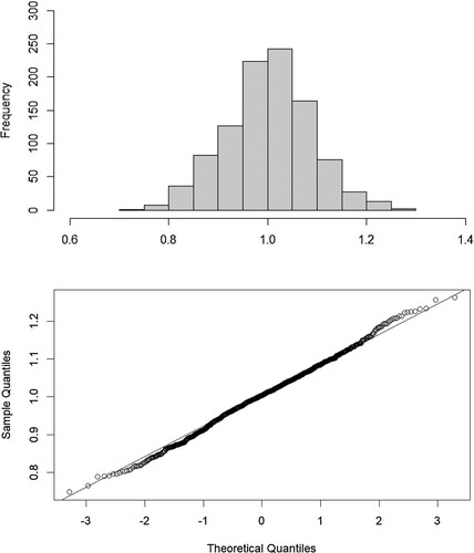
The histogram of 1000 values of $\hat{\mu }$ from simulation is shown in Figure 1, together with a Q–Q plot. The result suggests $\hat{\mu }$ is asymptotically normal, although such a theoretical result has not been established.

Figure 1. Histogram and Q–Q plot of 1000 simulated values of $\hat{\mu }$.

Acknowledgments

The authors would like to thank two anonymous referees for helpful comments and suggestions.

Disclosure statement

No potential conflict of interest was reported by the author(s).

Additional information

Funding

Jun Shao's research was partially supported by the National Natural Science Foundation of China [Grant Number 11831008] and the U.S. National Science Foundation [Grant Number DMS-1914411].

References

- Efron, B., & Tibshirani, R. J. (1993). An introduction to the bootstrap. New York: Chapman and Halll/CRC.
- Kim, H. J., Wang, Z., & Kim, J. K (2021). Survey data integration for regression analysis using model calibration. arXiv 2107.06448.
- Lohr, S. L., & Raghunathan, T. E. (2017). Combining survey data with other data sources. Statistical Science, 32(2), 293–312. https://doi.org/10.1214/16-STS584
- Merkouris, T. (2004). Combining independent regression estimators from multiple surveys. Journal of the American Statistical Association, 99(468), 1131–1139. https://doi.org/10.1198/016214504000000601
- Rao, J. N. K. (2021). On making valid inferences by integrating data from surveys and other sources. Sankhya B, 83(1), 242–272. https://doi.org/10.1007/s13571-020-00227-w
- Shao, J. (2003). Mathematical statistics. 2nd ed. Springer.
- Yang, S., & Kim, J. K. (2020). Statistical data integration in survey sampling: A review. Japanese Journal of Statistics and Data Science, 3(2), 625–650. https://doi.org/10.1007/s42081-020-00093-w
- Zhang, Y., Ouyang, Z., & Zhao, H. (2017). A statistical framework for data integration through graphical models with application to cancer genomics. The Annals of Applied Statistics, 11(1), 161–184. https://doi.org/10.1214/16-AOAS998
- Zieschang, K. D. (1990). Sample weighting methods and estimation of totals in the consumer expenditure survey. Journal of the American Statistical Association, 85(412), 986–1001. https://doi.org/10.1080/01621459.1990.10474969