Bayesian autoregressive adaptive refined descriptive sampling algorithm in the Monte Carlo simulation

Abstract

This paper deals with the Monte Carlo Simulation in a Bayesian framework. It shows the importance of the use of Monte Carlo experiments through refined descriptive sampling within the autoregressive model $X_t=\rho X_{t-1}+Y_t$, where $0<\rho <1$ and the errors $Y_t$ are independent random variables following an exponential distribution of parameter θ. To achieve this, a Bayesian Autoregressive Adaptive Refined Descriptive Sampling (B2ARDS) algorithm is proposed to estimate the parameters ρ and θ of such a model by a Bayesian method. We have used the same prior as the one already used by some authors, and computed their properties when the Normality error assumption is released to an exponential distribution. The results show that B2ARDS algorithm provides accurate and efficient point estimates.

Keywords:

• Monte Carlo simulation
• refined descriptive sampling methods
• variance reduction
• autoregressive process
• Bayesian estimation

1. Introduction

Time series are often used to model data in different areas of life. We can think of economic forecasts, the evolution of a biological system, time-stamped data from social media, E-commerce and sensor systems. The AutoRegressive (AR) model is the most widely used class of time series models, and particularly the first order AutoRegressive process denoted as AR(1).

On the other hand, the use of Bayesian inference has developed rapidly over the last decade in several fields including medicine (Ashby, 2006), genetics (Beaumont & Rannala, 2004), bioinformatics (Corander, 2006), econometrics (Geweke, 1999), etc.

Several works related to time series models have been treated by the Bayesian approach. Box et al. (1976), Monahan (1984) and Marriot and Smith (1992) discussed the Bayesian approach to analyse the AR models. Diaz and Farah (1981) devoted their work to a Bayesian technique for computing posterior analysis of an AR process in any arbitrary order. Amaral Turkmann (1990) considered a Bayesian study of an AR(1) model with exponential white noise based on a noninformative prior. Ghosh and Heo (2003) introduced a comparative study to some selected noninformative priors for the AR(1) model. Pereira and Amaral-Turkman (2004) developed a Bayesian analysis of a threshold AR model with exponential white noise.

Several Bayesian methods for estimating autoregressive parameters have been proposed by different authors; for instance, Albert and Chib (1993) and Barnett et al. (1996) proposed a Bayesian method via Gibbs sampling to estimate the parameters in an AR model. Ibazizen and Fellag (2003) proposed a Bayesian estimation of an AR(1) process with exponential white noise by using a noninformative prior, whereas Suparman and Rusiman (2018) proposed a hierarchical Bayesian estimation for stationary AR models using a reversible jump MCMC algorithm. However, Kumar and Agiwal (2019) proposed a Bayesian estimation for a full shifted Panel AR(1) time series model.

Bayesian inference is based on the posterior distribution, which can be interpreted as the result of the combination of two information sources: the information provided by the parameter which is contained in the prior distribution, and the information provided by the data which formalizes the likelihood function through the use of a given statistical model.

Posterior inference can be undertaken by applying classical Monte Carlo (MC) methods, which provide iterative algorithms that can generate approximate samples from the posterior distribution. These methods fall into two categories: the Markov Chain Monte Carlo (MCMC) methods such as Metropolis-Hastings and Gibbs algorithms (Smith & Robert, 1993), and the Monte Carlo (MC) method also known as Simple Random Sampling (SRS), for instance, Quasi Monte Carlo (Keller et al., 2008), Latin hypercube sampling (LHS) (Loh, 1996; Mckay et al., 1979; Stein, 1987), Descriptive Sampling (DS) (Saliby, 1990) as well as Refined Descriptive Sampling (RDS) (Tari & Dahmani, 2006). In the non-Bayesian estimation, the SRS is a widely used method in MC simulation. But unfortunately, the sampling method generates estimation errors, so it is not accurate enough. However, the RDS method (Aloui et al., 2015) has shown its effectiveness for several models and in various fields. For instance, in the field of medicine, Ourbih-Tari and Azzal (2017) proposed an RDS algorithm for a nonparametric estimation of the survival function using Kaplan Meier and Fleming Harrington estimators in a case study. In the field of engineering, Baghdali-Ourbih et al. (2017) have estimated the performance measures of the aggregate quarry of Bejaia city in Algeria, using a discrete-event simulation model. In the field of M/G/1 queuing models, M/M/1 retrial queues and M/G/1 retrial queues, simulation results using RDS outperform those obtained using the MC method (Idjis et al., 2017; Ourbih-Tari et al., 2017; Tamiti et al., 2018). Also, a comparison between RDS and LHS carried out on M/G/1 queues showed the efficiency of RDS over LHS (Boubalou et al., 2019). Since it is important to choose a sampling scheme that allows for a better parameter estimate while keeping the number of repetitions to a minimum, the RDS method is chosen for further work.

This paper will therefore explore the RDS method in a Bayesian sense by considering the AR(1) model, which has already been studied by Amaral Turkmann (1990) and, later on, by Ibazizen and Fellag (2003). For this purpose, we assume the noninformative prior given in Ibazizen and Fellag (2003) for the AR(1) process with exponential white noise. Then, we develop an algorithm for the estimation of AR(1) model parameters in a Bayesian context by using the most accurate sampling method as the RDS method. The proposed algorithm is called Bayesian Autoregressive Adaptive Refined Descriptive Sampling (B2ARDS).

Some details of the RDS method are given in Section 2. Then, in Section 3, the methodology from Bayesian perspective is explained. Section 4 is concerned with the Bayesian estimates of the AR(1) model parameters and their variances using the RDS method through the B2ARDS algorithm. Section 5 presents simulation experiments performed by using the R Package and corresponding results are summarized in Tables 1 and 2, and Figures 1 and 2. Finally, Section 6 concludes this paper.

Figure 1. Sequences of $\widehat{{\rho }_j}$ estimates for different true values of ρ. (a) $\rho =0.1$. (b) $\rho =0.3$. (c) $\rho =0.6$.

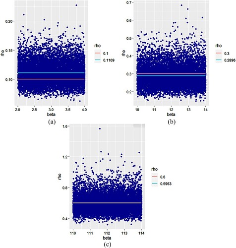
Figure 2. Sequences of $\widehat{{\theta }_j}$ estimates for $\theta =2.5$ and different values of ρ. (a) $\rho =0.1$. (b) $\rho =0.3$. (c) $\rho =0.6$.

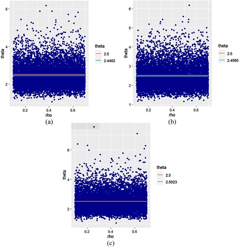
Table 1. Subsets of prime numbers size for a Gumbel distribution with mean $E\left(X\right)=0.577$, $p_1=7$, $p_2=11$ and $p_3=13$.

$\mathit{i}$	$r_i^1$	$x_i^1$	$\mathit{i}$	$r_i^2$	$x_i^2$	$\mathit{i}$	$r_i^3$	$x_i^3$
1	0.071	$-0$.970	1	0.045	$-1.129$	1	0.038	$-1.181$
2	0.214	$-0$.432	2	0.136	$-0$.689	2	0.115	$-0$.770
3	0.357	$-0$.029	3	0.227	$-0$.393	3	0.192	$-0$.501
4	0.500	0.367	4	0.318	$-0$.136	4	0.269	$-0$.272
5	0.643	0.817	5	0.409	0.112	5	0.346	$-0$.059
6	0.786	1.422	6	0.500	0.367	6	0.423	0.151
7	0.929	2.602	7	0.591	0.642	7	0.500	0.367
	${\hat{\theta }}_1$	0.539	8	0.682	0.960	8	0.577	0.601
			9	0.773	1.355	9	0.654	0.856
			10	0.864	1.920	10	0.731	1.159
			11	0.955	3.068	11	0.808	1.544
				${\hat{\theta }}_2$	0.553	12	0.885	2.099
						13	0.962	3.239
							${\hat{\theta }}_3$	0.556

Table 2. The observed mean of a Gumbel distribution using three regular subsets of prime number size.

j	1	2	3	Overall mean ($T_{\mathrm{R}\mathrm{D}\mathrm{S}}$)
${\hat{\theta }}_j$	0.539	0.553	0.556	0.551

2. The use of RDS

DS is known to have two problems. From a theoretical perspective, DS can be biased. More practically, its strict operation requires a prior knowledge of the required sample size. Based on this, RDS has been proposed to make DS safe, efficient and convenient. RDS makes DS safe by reducing substantially the risk of sampling bias, efficient by producing estimates with lower variances and convenient by removing the need to determine in advance the sample size. Not only this, but RDS beats DS in several comparisons and such is the case, on a flow shop system (Tari & Dahmani, 2005a) and a production system (Tari & Dahmani, 2005b). So, RDS is the preferred method when it comes to performing MC simulation.

2.1. Description of the method

RDS is based on a block of sub-samples of randomly generated prime number sizes, so it distributes RDS sample values from sub-samples at the request of the simulation. We stop the process of the generation of sample values when the simulation terminates, say when m prime numbers $p_j,$ $j=1,2,\dots ,m$, have been used, which derives m sub-runs.

The choice of primes in the RDS method as sub-sample sizes is motivated by the definition of primes since we must avoid integers having multiples, whether they are even or odd numbers. Indeed, if the underlying frequency is different from the sampling frequency (the product of primes) or a multiple of it, then the bias of the estimates will be insignificant as demonstrated in Tari and Dahmani (2006). This should ensure that the method reduces the sampling bias.

Remark: In the case of $\mathit{M}$ replicated simulation runs, the RDS method will distribute $\mathit{M}$ blocks defined by $m_1,m_2,\dots ,m_M$ primes which are not the same for all replicated simulation runs.

2.2. RDS sample values

Formally, in an RDS run defined by a sample of size $n=\sum _{j=1}^m{p}_j$, the sample values drawn from the input real-valued random variable X having F as the cumulative distribution are given by the following formulas: (1) $x_i^j=F^{-1}\left(R_i^j\right)\mathrm{f}\mathrm{o}\mathrm{r}i=1,2,\dots ,p_j\mathrm{a}\mathrm{n}\mathrm{d}j=1,2,\dots ,m,$(1) where for any $j=1,2,\dots ,m,$ the values of each sub-sample $(R_i^j,i=1,2,\dots ,p_j)$ are randomly selected without replacement from the regular numbers of the following sub-set (2) $(r_i^j=\frac{(i-0.5)}{p_j},i=1,2,\dots ,p_j)$(2) and such $r_i^j$ is the midpoint of the $p_j$ subintervals in which the interval $[0,1]$ is subdivided. The primes $p_j,j=1,2,\dots ,m$, are randomly generated between 7 and a given value fixed by the user.

2.3. The estimator of RDS

The j-th sub-run generating $p_j$ values of the input random variable X leads to the following estimate of the parameter θ (3) ${\hat{\theta }}_j=\frac{1}{p_j}\sum _{i=1}^{p_j}h\left(x_i^j\right).$(3) Therefore, in a given run, the use of refined descriptive sample of size $n=\sum _{j=1}^m{p}_j$ leads to the following sampling estimate of θ defined by the average of those estimates observed on different sub-runs: (4) $T_{\mathrm{R}\mathrm{D}\mathrm{S}}=\frac{1}{n}\sum _{j=1}^m\sum _{i=1}^{p_j}h\left(x_i^j\right),$(4) where h is the simulation function.

2.4. Example

We illustrate the method by taking the Gumbel distribution and the prime numbers $p_1=7$, $p_2=11$ and $p_3=13$. The values of the variable are simulated by the formula $x_i=-\ln (-\ln (r_i\left)\right)$, $i=1,2,\dots ,p_j$ and $j=1,2,\dots ,m$. When m = 3, the obtained sub-sets and sub-samples are given in Table 1 using the formulas (2(2) $(r_i^j=\frac{(i-0.5)}{p_j},i=1,2,\dots ,p_j)$(2) ) and (1(1) $x_i^j=F^{-1}\left(R_i^j\right)\mathrm{f}\mathrm{o}\mathrm{r}i=1,2,\dots ,p_j\mathrm{a}\mathrm{n}\mathrm{d}j=1,2,\dots ,m,$(1) ), respectively, together with the observed mean $\left({\hat{\theta }}_j\right)$ in each sub-run using the formula (3(3) ${\hat{\theta }}_j=\frac{1}{p_j}\sum _{i=1}^{p_j}h\left(x_i^j\right).$(3) ), while the overall mean computed at the end of the run is given in Table 2 using the formula (4(4) $T_{\mathrm{R}\mathrm{D}\mathrm{S}}=\frac{1}{n}\sum _{j=1}^m\sum _{i=1}^{p_j}h\left(x_i^j\right),$(4) ).

3. Monte Carlo methods from a Bayesian perspective

We consider a random vector Y having a probability density function $f(y\mid \theta )$, where θ is a vector of unknown parameters. The Bayesian statistic considers θ as a random vector of density $\pi \left(\theta \right)$ called prior law of θ.

In a Bayesian sense, any inference is based on the computation of the posterior distribution which is the conditional distribution of the random vector θ knowing y and is denoted by its probability density $\pi (\theta \mid y)$. Bayesian estimator of the parameter θ is constructed from the posterior distribution $\pi (\theta \mid y)$ by minimizing an appropriate loss function. Most Bayesian estimators have the form of $E_{\pi }\left[h\right(\theta \left)\right]$, where $E_{\pi }$ denotes the mathematical expectation of the posterior distribution $\pi (\theta \mid y)$.

A major difficulty in an estimation by the Bayesian approach, is the explicit computation of the posterior distribution as soon as the number of parameters exceeds two. Also computing $E_{\pi }\left[h\right(\theta \left)\right]$ can be very difficult even if the law is known. Thus, several approximation methods such as the MC and MCMC methods are proposed in the literature. The latter allows for the estimation of moments of any order of random variables, too complex to be studied analytically, using iterative generation algorithms.

The Monte Carlo method is a numerical method of solving problems using random numbers. It is one of the most popular mathematical tools with a very wide scope, like differential equation integration, fluid mechanics equations, financial mathematics, particles transport and matrix inversion.

In a Bayesian sense, the Monte Carlo method consists in estimating $I_h=E_{\pi }\left[h\right(\theta \left)\right]=\underset{\theta }{\int }h\left(\theta \right)\pi (\theta \mid y)\mathrm{d}\theta$by ${\hat{I}}_h=\frac{1}{n}\underset{i=1}{\sum ^n}h\left({\theta }_i\right),$where ${\theta }_1,{\theta }_2,\dots ,{\theta }_n$ are independent and identically distributed i.i.d. random variables according to $\pi (\theta \mid y)$. The strong law of large numbers ensures that ${\hat{I}}_h$ converges almost surely to $I_h$ when $\mathit{n}$ tends to infinity.

4. The use of RDS for the simulation of the proposed model

4.1. Presentation of the model

Consider the first order autoregressive process defined by (5) $X_t=\rho X_{t-1}+Y_t,t=\dots ,-1,0,1,\dots ,$(5) where $0<\rho <1$ and the $Y_t$'s are i.i.d. random variables with the exponential distribution exp$\left(\theta \right)$ of parameter θ having a density $f\left(y\right)=\theta \exp (-\theta y)I_{(0,\mathrm{\infty })}\left(y\right),\theta >0.$$X_1$ is assumed to be distributed according to exp$\left(\right(1-\rho \left)\theta \right)$ such that the process is mean stationary.

The likelihood function based on the observations $x=\{x_1,x_2,\dots ,x_n\}$ is $f(x\mid \theta ,\rho )=(1-\rho ){\theta }^n{\mathrm{e}}^{-\theta (n\overline{x}-\rho S)}{I}_A\left(x\right),$where $A=\{x:x_1>0,x_t-\rho x_{t-1}\ge 0,t=2,\dots ,n\},n\overline{x}=\underset{i=1}{\sum ^n}{x}_t$and (6) $S=n\overline{x}-(x_n-x_1).$(6) The Maximum Likelihood Estimators (MLE) of ρ and θ are introduced by Andel (1988) , respectively as follows: (7) $\begin{array}{rl}& {\rho }_0=min(1,\frac{x_2}{x_1},\dots ,\frac{x_n}{x_1}),\end{array}$(7) (8) $\begin{array}{rl}& {\theta }_0=\frac{n}{n\overline{x}-{\rho }_{0}S}.\end{array}$(8) The model given by (5(5) $X_t=\rho X_{t-1}+Y_t,t=\dots ,-1,0,1,\dots ,$(5) ) was processed using a Bayesian approach by Amaral Turkmann (1990). The author's study is based on a noninformative prior defined as follows: (9) $\pi (\theta ,\rho )\propto \frac{1}{\theta (1-\rho )}{I}_{[0,\mathrm{\infty }]\times [0,1)}(\theta ,\rho ).$(9) The author derived the Bayes estimators of the independent parameters ρ and θ as follows: ${\rho }^B=\frac{{\rho }_0}{n-2}(\frac{n-1}{1-r^{n-1}}-\frac{1}{1-r}),$and ${\theta }^B=\frac{n-1}{n\overline{x}r}\frac{1-r^n}{1-r^{n-1}},$where $r=1-{\rho }_0\left(\frac{S}{n\overline{x}}\right)$ such that 0<r<1.

Ibazizen and Fellag (2003) proposed a Bayesian analysis of the model (5(5) $X_t=\rho X_{t-1}+Y_t,t=\dots ,-1,0,1,\dots ,$(5) ) by using a more general noninformative prior defined by (10) $\pi (\theta ,\rho ,\text{β})\propto \frac{1}{\theta }\frac{{\rho }^{\text{β}-1}}{1-\rho }{I}_{[0,\mathrm{\infty }]\times [0,1)}(\theta ,\rho ),\text{β}>0$(10) which includes the formula (9(9) $\pi (\theta ,\rho )\propto \frac{1}{\theta (1-\rho )}{I}_{[0,\mathrm{\infty }]\times [0,1)}(\theta ,\rho ).$(9) ) as a special case ($\text{β}=1$). For θ, the prior (7) is proportional to the scale parameter $1/\theta$ and for ρ, it is a special case of the beta distribution.

The authors have derived Bayesian estimators given below, but their formulas are complicated for computation. So, simulation experiments were carried out and the obtained results were compared to the MLE. $\begin{array}{rl}{\hat{\rho }}_B\left(\text{β}\right)& =\frac{{}_2{F}_1(\text{β}+1,n,\text{β}+2;1-r){\rho }_0\text{β}}{{}_2{F}_1(\text{β},n,\text{β}+1;1-r)(\text{β}+1)},\\ {\hat{\theta }}_B\left(\text{β}\right)& =\frac{{}_2{F}_1(\text{β},n+1,\text{β}+1;1-r)}{\overline{x}{}_2{F}_1(\text{β},n,\text{β}+1;1-r)},\end{array}$where $\begin{array}{rl}{}_2{F}_1(a,b,c;x)& =\underset{m=0}{\sum ^{\mathrm{\infty }}}\frac{(a,m)(b,m)x^m}{(c,m)m!}\\ & ={\int }_0^1\frac{u^{a-1}(1-u{)}^{c-a-1}(1-xu{)}^{-b}}{\mathcal{B}(a,c-a)}\mathrm{d}u\mathrm{f}\mathrm{o}\mathrm{r}|x|<1\end{array}$is the Gauss hypergeometric function of parameters $(\mathit{a},\mathit{b},\mathit{c})$.

We note that to compute the latter, the Pochhammer coefficients $(t,m)$ for t = a, b and c are defined as follows $(t,m)=\mathrm{\Gamma }(t+m)/\mathrm{\Gamma }\left(t\right)\mathrm{f}\mathrm{o}\mathrm{r}m⩾1\mathrm{a}\mathrm{n}\mathrm{d}(t,0)=1,$where Γ and $\mathcal{B}$ represent symbols of the usual functions Gamma and Beta, respectively.

This paper focuses on the Bayesian estimation of ρ and θ using the most accurate RDS method to generate numbers for the simulation, where the prior distribution of ρ and θ is the one given in (10(10) $\pi (\theta ,\rho ,\text{β})\propto \frac{1}{\theta }\frac{{\rho }^{\text{β}-1}}{1-\rho }{I}_{[0,\mathrm{\infty }]\times [0,1)}(\theta ,\rho ),\text{β}>0$(10) ) because it is the most general noninformative prior.

4.2. Bayesian estimation of ρ and θ using the RDS method

Suppose that our data consists of the first $\mathit{n}$ observations $x=(x_1,x_2,\dots ,x_n)$.

By using the prior in (10(10) $\pi (\theta ,\rho ,\text{β})\propto \frac{1}{\theta }\frac{{\rho }^{\text{β}-1}}{1-\rho }{I}_{[0,\mathrm{\infty }]\times [0,1)}(\theta ,\rho ),\text{β}>0$(10) ) and the Bayes theorem, we get the following posterior: (11) $\pi (\theta ,\rho \mid x)=\frac{{\rho }^{\text{β}-1}{\theta }^{n-1}{\mathrm{e}}^{-\theta (n\overline{x}-\rho S)}{I}_{(0,\mathrm{\infty })\times [0,{\rho }_0]}(\theta ,\rho )}{\mathrm{\Gamma }\left(n\right){\int }_0^{{\rho }_0}{\rho }^{\text{β}-1}(n\overline{x}-\rho S{)}^{-n}\mathrm{d}\rho },$(11) which is proportional to (12) ${\rho }^{\text{β}-1}{\theta }^{n-1}{\mathrm{e}}^{-\theta (n\overline{x}-\rho S)}{I}_{(0,\mathrm{\infty })\times [0,{\rho }_0]}(\theta ,\rho ).$(12) Knowing that the parameters ρ and θ are independent, the conditional posterior distributions of ρ and θ are respectively (13) $F\left(\rho \right)=\pi (\rho \mid x,\theta )\propto {\rho }^{\text{β}-1}{\mathrm{e}}^{\theta \rho S}$(13) and (14) $H\left(\theta \right)=\pi (\theta \mid x,\rho )\propto {\theta }^{n-1}{\mathrm{e}}^{-\theta (n\overline{x}-\rho S)}.$(14) The use of RDS method requires the computation of the inverse cumulative distribution functions $F^{-1}$ and $H^{-1}$, so we put $\begin{array}{rl}& R_1=F\left(\rho \right)={\rho }^{\text{β}-1}{\mathrm{e}}^{\theta \rho S},\\ & R_2=H\left(\theta \right)={\theta }^{n-1}{\mathrm{e}}^{-\theta (n\overline{x}-\rho S)}.\end{array}$The inversion method leads to the following ρ and θ values of the conditional posterior distributions which will be used for the generation of observations: (15) $\rho =F^{-1}\left(R_1\right)=\frac{1}{\theta S}\ln \left(\frac{R_1}{{\rho }^{\text{β}-1}}\right)$(15) and (16) $\theta =H^{-1}\left(R_2\right)=\frac{1}{n\overline{x}-\rho S}\ln \left(\frac{{\theta }^{n-1}}{R_2}\right),$(16) where the variables $R_1$ and $R_2$ following $\mathcal{U}[0,1]$ are generated using the RDS algorithm given in subsection 4.3 (see Appendix 1 for the generation of the ρ values and Appendix 2 for the generation of the θ values).

4.3. Adaptive RDS algorithm to AR(1) model from the Bayesian perspective by using the R language

In this section, we present a new Bayesian Adaptive AR(1) RDS (B2ARDS) algorithm to estimate the parameters of the model given in (2).

Data structure

For each input random variable, we define a record with the following structure.

N: an integer defining the number of replications.

n: an integer defining the sample size.

p: a prime number defining the size of the sub-sample.

P: an array of generated primes.

r: an array $[1,\dots ,p]$ of real numbers containing the sub-set of regular numbers.

R: an array of mixed values of $\mathit{r}$.

$x_i,i=1,\dots ,n$: simulated observations from the AR(1) model.

ρ: an array $[1,\dots ,p]$ containing the generated RDS sub-sample values, issued from the ρ distribution.

θ: an array $[1,\dots ,p]$ containing the generated RDS sub-sample values, issued from the θ distribution.

Algorithm

1. Initialization for the experiment of N replicated runs.

2. Initialization of the run defined by the sample size n.

3. Simulate samples of n observations $x_1,x_2,\dots ,x_n$ from the model $\left(5\right)$ by using the command : $>x=\mathrm{a}\mathrm{r}\mathrm{i}\mathrm{m}\mathrm{a}.\mathrm{s}\mathrm{i}\mathrm{m}\left(\mathrm{l}\mathrm{i}\mathrm{s}\mathrm{t}\right(ar=\rho ),n,\mathrm{i}\mathrm{n}\mathrm{n}\mathrm{o}\mathrm{v}=r\mathrm{e}\mathrm{x}\mathrm{p}(n,\mathrm{r}\mathrm{a}\mathrm{t}\mathrm{e}=\theta \left)\right).$

4. Compute the values $\overline{x}$ and S, using formula (6(6) $S=n\overline{x}-(x_n-x_1).$(6) ) and $n\overline{x}-\rho S$.

5. Before each simulation run, generate a vector of prime numbers smaller than the sample size n and store them in a vector P.

6. Randomize the vector P.

7. Compute the sum of primes successively and stop when the sum is $⩾n$ and collect the number of primes m.

8. Initialization of the sub-run defined by the prime p.

9. For each prime number $p_j$, $j=1,\dots ,m$, we do the following sub-run.

   	(f1)	Compute the regular numbers $r_i,i=1,\dots ,p_j$ using the formula (2(2) $(r_i^j=\frac{(i-0.5)}{p_j},i=1,2,\dots ,p_j)$(2) ) and store them in an array r.
   	(f2)	Randomize the $r_i$ by the command: $>R=\mathrm{s}\mathrm{a}\mathrm{m}\mathrm{p}\mathrm{l}\mathrm{e}\left(r\right)$ and store them in an array R.
   	(f3)	Generate the observations ${\rho }_i=F^{-1}\left(R_i\right)$ and ${\theta }_i=H^{-1}\left(R_i\right)$, $i=1,\dots ,p_j$ and store them respectively in arrays ρ and θ.
   	(f4)	Compute the simulation estimates $\widehat{{\rho }_j}$ and $\widehat{{\theta }_j}$ in the j-th sub-run such that $\widehat{{\rho }_j}=\frac{1}{p_j}\underset{i=1}{\sum ^{p_j}}{\rho }_i,\widehat{{\theta }_j}=\frac{1}{p_j}\underset{i=1}{\sum ^{p_j}}{\theta }_i.$

10. Compute the final RDS estimates of ρ and θ using the output sample of size $\sum _{j=1}^m{p}_j$ respectively as

    ${\hat{\rho }}_{\mathrm{R}\mathrm{D}\mathrm{S}}=\frac{\underset{j=1}{\sum ^m}{p}_j\widehat{{\rho }_j}}{\underset{j=1}{\sum ^m}{p}_j},{\hat{\theta }}_{\mathrm{R}\mathrm{D}\mathrm{S}}=\frac{\underset{j=1}{\sum ^m}{p}_j\widehat{{\theta }_j}}{\underset{j=1}{\sum ^m}{p}_j}.$

5. Results and discussion

5.1. Simulation study

In the following, we present a simulation study using the R language. We generate samples of n observations $x_1,x_2,\dots ,x_n$ from the AR(1) model given in $\left(5\right)$ which provides the values of $\overline{x}$, S and $n\overline{x}-\rho S$. Three simulation experiments were carried out with different sample sizes such as $n=20,30,40$ for each selected ρ value such as 0.1, 0.3, 0.6, respectively. The proposed B2ARDS algorithm is used to compute the RDS estimates $\hat{\rho }$ and $\hat{\theta }$ together with their variances. Note that, in the estimation of ρ, different values of β are taken from one experiment to another in order to study the effect of varying β on the Bayesian estimates $\hat{\rho }$ and $\hat{\theta }$. A summary of results is given in Tables 1 and 2, together with ${\rho }_0$ and ${\theta }_0$, computed using formulas (7(7) $\begin{array}{rl}& {\rho }_0=min(1,\frac{x_2}{x_1},\dots ,\frac{x_n}{x_1}),\end{array}$(7) ) and (8(8) $\begin{array}{rl}& {\theta }_0=\frac{n}{n\overline{x}-{\rho }_{0}S}.\end{array}$(8) ), respectively (see Appendix 3 for details).

At the end of the simulation, we collect the sequences of $\widehat{{\rho }_j}$ and $\widehat{{\theta }_j}$ estimates resulting from step $\left(f_4\right)$ of the proposed algorithm. For N=10,000 replications, sequences of $\widehat{{\rho }_j}$ estimates for initial values of $\rho =0.1,0.3,0.6$ are represented in Figure 1 while Figure 2 represents sequences of $\widehat{{\theta }_j}$ estimates for the same ρ values as in Figure 1.

5.2. Interpretation of tables

According to the simulation results given in Tables 3 and 4, we have very small variances (given in parentheses). So, we can say that the sequences of RDS values ${\rho }_i$ and ${\theta }_i$, generated by the proposed B2ARDS algorithm are homogeneous. Also, in each case ${\hat{\rho }}_{\mathrm{R}\mathrm{D}\mathrm{S}}$ is too close to the true value of ρ while, for some values of β, ${\hat{\rho }}_{\mathrm{R}\mathrm{D}\mathrm{S}}$ is closer to the true value than ${\rho }_0$. It can be seen in Figure 1 that when ρ is close to 0, the best values of ${\hat{\rho }}_{\mathrm{R}\mathrm{D}\mathrm{S}}$ are obtained when $\text{β}\in [2.5,16]$; while, when ρ is close to 1, the best values of ${\hat{\rho }}_{\mathrm{R}\mathrm{D}\mathrm{S}}$ are obtained for high values of β ($\text{β}\in [50,111]$). So, there are some values for ρ and β for which the resulting Bayesian estimate is ideal in accuracy.

Table 3. The simulated estimator ${\hat{\rho }}_{\mathrm{R}\mathrm{D}\mathrm{S}}$ and its variance for $\theta =2.5$ and for various values of ρ, n and β. Variances in parentheses.

$\rho =0.1$
		${\hat{\rho }}_{\mathrm{R}\mathrm{D}\mathrm{S}}$
n	${\rho }_0$	$\text{β}=2$	$\text{β}=2.5$	$\text{β}=3$	$\text{β}=3.5$
20	0.1067	0.0798 (0.0032)	0.1188 (0.0009)	0.1886 (0.0021)	0.2284 (0.0032)
30	0.1075	0.0445 (0.00008)	0.0812 (0.0002)	0.1144 (0.0005)	0.1499 (0.0009)
40	0.1062	0.0306 (0.00002)	0.0581 (0.00009)	0.0846 (0.0002)	0.1107 (0.0003)
$\rho =0.3$
		${\hat{\rho }}_{\mathrm{R}\mathrm{D}\mathrm{S}}$
n	${\rho }_0$	$\text{β}=7.5$	$\text{β}=8$	$\text{β}=8.5$	$\text{β}=9$
20	0.3035	0.2815 (0.0078)	0.3047 (0.0084)	0.3009 (0.0056)	0.3232 (0.0063)
n	${\rho }_0$	$\text{β}=10.5$	$\text{β}=11$	$\text{β}=11.5$	$\text{β}=12$
30	0.3030	0.2633 (0.0030)	0.2736 (0.0032)	0.2947 (0.0034)	0.3034 (0.0036)
n	${\rho }_0$	$\text{β}=15$	$\text{β}=15.5$	$\text{β}=16.0$	$\text{β}=16.5$
40	0.3080	0.2926 (0.0026)	0.3006 (0.0026)	0.3125 (0.0028)	0.3236 (0.0031)
$\rho =0.6$
		${\hat{\rho }}_{\mathrm{R}\mathrm{D}\mathrm{S}}$
n	${\rho }_0$	$\text{β}=50$	$\text{β}=50.5$	$\text{β}=55$	$\text{β}=55.5$
20	0.6435	0.5980(0.0559)	0.6017 (0.0516)	0.6191 (0.0487)	0.6365 (0.0423)
n	${\rho }_0$	$\text{β}=75.5$	$\text{β}=80$	$\text{β}=80.5$	$\text{β}=85.5$
30	0.6204	0.5600 (0.0199)	0.5960 (0.0051)	0.6057 (0.0209)	0.6283 (0.0201)
n	${\rho }_0$	$\text{β}=110$	$\text{β}=110.5$	$\text{β}=111$	$\text{β}=111.5$
40	0.6136	0.6002 (0.0124)	0.6009 (0.0127)	0.6014 (0.0123)	0.6013 (0.0121)

Table 4. The simulated estimator ${\hat{\theta }}_{\mathrm{R}\mathrm{D}\mathrm{S}}$ and its variance for $\theta =2.5$ and for different values of ρ and n. Variances are given in parentheses.

n	ρ	${\theta }_0$	${\hat{\theta }}_{\mathrm{R}\mathrm{D}\mathrm{S}}$
20	0.1	2.5252	2.4405 (0.3438)
	0.3	2.5216	2.4534 (0.3347)
	0.6	2.5140	2.4970 (0.3742)
30	0.1	2.5063	2.3841 (0.2141)
	0.3	2.5551	2.4140 (0.2073)
	0.6	2.5840	2.4293 (0.2189)
40	0.1	2.4949	2.3522 (0.1453)
	0.3	2.6455	2.3609 (0.1588)
	0.6	2.4982	2.3906 (0.1608)

For ${\hat{\theta }}_{\mathrm{R}\mathrm{D}\mathrm{S}}^B$, the results in Table 4 and Figure 2 also prove that, for each case, the Bayesian estimate of θ is very close to the true value of θ and for some cases (n=20 and $\rho =0.6$), it is a better estimate than ${\theta }_0$. We notice here that the best values of ${\hat{\theta }}_{\mathrm{R}\mathrm{D}\mathrm{S}}^B$ are obtained when ρ is close to 1.

5.3. Interpretation of figures

In each figure, the red line represents the true value of the parameter, while the green line represents the value of the resulting ${\hat{\rho }}_{\mathrm{R}\mathrm{D}\mathrm{S}}$ and ${\hat{\theta }}_{\mathrm{R}\mathrm{D}\mathrm{S}}$ estimators for the j-th sub-run. We notice that the points which represent the estimates $\widehat{{\rho }_j}$ and $\widehat{{\theta }_j}$ are concentrated in a given band for all figures and nearly all points are concentrated around their mean, which represents in a Bayesian sense the resulting ${\hat{\rho }}_{\mathrm{R}\mathrm{D}\mathrm{S}}$ and ${\hat{\theta }}_{\mathrm{R}\mathrm{D}\mathrm{S}}$ estimators of the parameters ρ and θ, respectively. We can see from all figures that the resulting estimate is not only very close to the true value of the parameter in each case, but it coincides with it in some cases (Figure 1 (c) and Figure 2 (c)).

6. Conclusion

The proposed algorithm B2ARDS has allowed us to generate refined descriptive samples from input random variables for Bayesian estimation of AR(1) parameter in Monte Carlo simulation using the R software. As a consequence and apart from its already proved efficiency in the classical sense, we argue that the RDS method performs well even in a Bayesian context and allows the estimation of the AR(1) parameter using the Bayesian approach.

Disclosure statement

No potential conflict of interest was reported by the author(s).

Appendices

Appendix 1 Computation of the ρ values

According to formula (13(13) $F\left(\rho \right)=\pi (\rho \mid x,\theta )\propto {\rho }^{\text{β}-1}{\mathrm{e}}^{\theta \rho S}$(13) ), we have $\pi (\rho \mid x,\theta )\propto {\rho }^{\text{β}-1}{\mathrm{e}}^{\theta \rho S}.$By applying the inversion method, we get $F^{-1}\left(R_1\right)=inf\{\rho :F(\rho )\ge R_1\}$ where $R_1\sim \mathcal{U}[0,1]$.

We put $R_1=F\left(\rho \right)={\rho }^{\text{β}-1}{\mathrm{e}}^{\theta \rho S}$, such that $R_1\sim \mathcal{U}[0,1]$.

Then $\begin{array}{rl}\ln R_1& =\ln \left({\rho }^{\text{β}-1}{\mathrm{e}}^{\theta \rho S}\right)\\ & =\ln \left({\rho }^{\text{β}-1}\right)+\ln \left({\mathrm{e}}^{\theta \rho S}\right)\\ & =\ln \left({\rho }^{\text{β}-1}\right)+\theta \rho S\end{array}$and $\theta \rho S=\ln R_1-\ln \left({\rho }^{\text{β}-1}\right)=\ln \left(\frac{R_1}{{\rho }^{\text{β}-1}}\right),$where $\rho =F^{-1}\left(R_1\right)=\frac{1}{\theta S}\ln \left(\frac{R_1}{{\rho }^{\text{β}-1}}\right).$

Appendix 2

Computation of the θ values

According to formula (14(14) $H\left(\theta \right)=\pi (\theta \mid x,\rho )\propto {\theta }^{n-1}{\mathrm{e}}^{-\theta (n\overline{x}-\rho S)}.$(14) ), we have $\pi (\theta \mid x,\rho )\propto {\theta }^{n-1}{\mathrm{e}}^{-\theta (n\overline{x}-\rho S)}.$We put $R_2=H\left(\theta \right)={\theta }^{n-1}{\mathrm{e}}^{-\theta (n\overline{x}-\rho S)}$, such that $R_2\sim \mathcal{U}[0,1]$.

Then $\begin{array}{rl}\ln R_2& =\ln \left({\theta }^{n-1}{\mathrm{e}}^{-\theta (n\overline{x}-\rho S)}\right)\\ & =\ln \left({\theta }^{n-1}\right)+\ln \left({\mathrm{e}}^{-\theta (n\overline{x}-\rho S)}\right)\\ & =\ln \left({\theta }^{n-1}\right)-\theta (n\overline{x}-\rho S)\end{array}$and $\theta (n\overline{x}-\rho S)=\ln \left({\theta }^{n-1}\right)-\ln R_2=\ln \left(\frac{{\theta }^{n-1}}{R_2}\right),$where $\theta =\frac{1}{n\overline{x}-\rho S}\ln \left(\frac{{\theta }^{n-1}}{R_2}\right),$so $\theta =H^{-1}\left(R_2\right)=\frac{1}{n\overline{x}-\rho S}\ln \left(\frac{{\theta }^{n-1}}{R_2}\right).$

Appendix 3

Computation of the MLE ${\rho }_0$ and ${\theta }_0$ by using the R language

We used the following programme to compute the MLE ${\rho }_0$ and ${\theta }_0$.

Program

$>n=30$;   $\rho =0.6$;    $\theta =2.5$

$>x=\mathrm{a}\mathrm{r}\mathrm{i}\mathrm{m}\mathrm{a}.\mathrm{s}\mathrm{i}\mathrm{m}\left(\mathrm{l}\mathrm{i}\mathrm{s}\mathrm{t}\right(ar=\rho ),n,\mathrm{i}\mathrm{n}\mathrm{n}\mathrm{o}\mathrm{v}=r\mathrm{e}\mathrm{x}\mathrm{p}(n,\mathrm{r}\mathrm{a}\mathrm{t}\mathrm{e}=\theta \left)\right)$

$>mx=\mathrm{m}\mathrm{e}\mathrm{a}\mathrm{n}\left(x\right)$

$>S=n\ast mx-\left(x\right[n]-x[1\left]\right)$

$>\mathrm{f}\mathrm{o}\mathrm{r}(i\mathrm{i}\mathrm{n}2:n)s\left[i\right]=x\left[i\right]/x[i-1]$

$>s$

$>\rho =min(1,s)$

$>\rho$

$>\theta =n/(n\ast mx-\rho \ast S)$

$>\theta$

References

- Albert, J. H., & Chib, S. (1993). Bayes inference via Gibbs sampling of autoregressive time series subject to Markov mean and variance shifts. Journal of Business
- Aloui, A., Zioui, A., Ourbih-Tari, M., & Alioui, A. (2015). A general purpose module using refined descriptive sampling for installation in simulation systems. Computational Statistics, 30(2), 477–490. https://doi.org/10.1007/s00180-014-0545-7
- Amaral Turkmann, M. A. (1990). Bayesian analysis of an autoregressive process with exponential white noise. Statistics, 21(4), 601–608. https://doi.org/10.1080/02331889008802270
- Andel, J. (1988). On AR(1) processes with exponential white noise. Communications in Statistics - Theory and Methods, 17(5), 1481–1495. http://doi.org/10.1080/03610928808829693
- Ashby, D. (2006). Bayesian statistics in medicine: A 25 year review. Statistics in Medicine, 25(21), 3589–3631. https://doi.org/10.1002/sim.v25:21
- Baghdali-Ourbih, L., Ourbih-Tari, M., & Dahmani, A. (2017). Implementing refined descriptive sampling into three phase discrete-event simulation models. Communications in Statistics : Simulation and Computation. Taylor and Francis, 46(5), 4035–4049. https://doi.org/10.1080/03610918.2015.1085557
- Barnett, G., Koln, R., & Sheather, S. (1996). Bayesian estimation of an autoregressive model using Markov chain Monte Carlo. Journal of Econometrics, 74(2), 237–254. https://doi.org/10.1016/0304-4076(95)01744-5
- Beaumont, M. A., & Rannala, B. (2004). The Bayesian revolution in genetics. Nature Reviews Genetics, 5(4), 251–261. https://doi.org/10.1038/nrg1318
- Boubalou, M., Ourbih-Tari, M., Aloui, A., & Zioui, A. (2019). Comparing M/G/1 queue estimators in Monte Carlo simulation through the tested generator getRDS and the proposed getLHS using variance reduction. Monte Carlo Methods and Applications, 25(2), 177–186. https://doi.org/10.1515/mcma-2019-2033
- Box, G., Jinkins, G., & Reinsel, G. (1976). Time series analysis: Forecasting and control. John Wiley and Sons.
- Corander, J. (2006). Is there a real Bayesian revolution in pattern recognition for bioinformatics. Current Bioinformatics, 1(2), 161–165. https://doi.org/10.2174/157489306777011932
- Diaz, J., & Farah, J. (1981). Bayesian identification of autoregressive processes. In Proceedings of the S.L, 22nd NBER-NSF. Seminar on Bayesian inference in econometrics.
- Geweke, J. (1999). Using simulation methods for Bayesian econometric models. Inference, Development, and Communication Econometric Reviews, 18(1), 1–126. https://doi.org/10.1080/07474939908800428
- Ghosh, M., & Heo, J. (2003). Default Bayesian priors for regression models with first-order autoregressive residuals. Journal of Time Series Analysis, 24(3), 269–282. https://doi.org/10.1111/jtsa.2003.24.issue-3
- Ibazizen, M., & Fellag, H. (2003). Bayesian estimation of an AR(1) process with exponential white noise. Journal of Theoretical and Applied Statistics, 37(5), 365–372. https://doi.org/10.1080/0233188031000078042
- Idjis, K., Ourbih-Tari, M., & Baghdali-Ourbih, L. (2017). Variance reduction in M/M/1 retrial queues using refined descriptive sampling. Communications in Statistics – Simulation and Computation, 46(6), 5002–5020. https://doi.org/10.1080/03610918.2016.1140778
- Keller, A., Heinrich, S., & Niederreiter, H. (2008). Monte Carlo and quasi Monte Carlo methods. Springer.
- Kumar, J., & Agiwal, V. (2019). Bayesian estimation for fully shifted panel AR(1) time series model. Thai Journal of Mathematics, 17, 167–183. https://thaijmath.in.cmu.ac.th
- Loh, W. L. (1996). On latin hypercube sampling. Annals of Statistics, 24(5), 2058–2080. https://doi.org/10.1214/aos/1069362310
- Marriot, J., & Smith, A. (1992). Reparametrization aspects of numerical Bayesian methods for autoregressive moving average models. Journal of Time Series Analysis, 13(4), 307–331. https://doi.org/10.1111/j.1467-9892.1992.tb00111.x
- Mckay, M. D., Conover, W. J., & Beckman, R. J. (1979). A comparison of three methods for selecting values of input variables in the analysis of output from a computer code. Technometrics, 21(2), 239–245. https://doi.org/10.2307/1268522
- Monahan, J. (1984). Fully Bayesian analysis of ARMA time series models. Journal of Econometrics, 21(3), 307–331. https://doi.org/10.1016/0304-4076(83)90048-9
- Ourbih-Tari, M., & Azzal, M. (2017). Survival function estimation with non parametric adaptative refined descriptive sampling algorithm : A case study. Communication in Statistics-Theory and Methods, 46(12), 5840–5850. https://doi.org/10.1080/03610926.2015.1065328
- Ourbih-Tari, M., Zioui, A., & Aloui, A. (2017). Variance reduction in the simulation of a stationary M/G/1 queuing system using refined descriptive sampling. Communication in Statistics-Simulation and Computation, 46(5), 3504–3515. https://doi.org/10.1080/03610918.2015.1096374
- Pereira, I., & Amaral-Turkman, M. A. (2004). Bayesian prediction in threshold autoregressive models with exponential white noise. sociedad De Estadistica E Investigacion Operativa, 13(1), 45–64. https://doi.org/10.1007/BF02603000
- Saliby, E. (1990). Descriptive sampling: A better approach to Monte Carlo simulation. Journal of the Operational Research Society, 41(12), 1133–1142. https://doi.org/10.1057/jors.1990.180
- Smith, A. F. M., & Robert, G. O. (1993). Bayesian computation via the Gibbs sampler and related Markov chain Monte Carlo methods. Journal of the Royal Statistical Society, 5(5), 3–23. https://doi.org/10.1111/j.2517-6161.1993.tbo1466.X
- Stein, M. (1987). Large sample properties of simulations using latin hypercube sampling. Technometrics, 29(2), 143–151. https://doi.org/10.1080/00401706.1987.10488205
- Suparman, S., & Rusiman, M. S. (2018). Hierarchical Bayesian estimation for stationary autoregressive models using reversible jump MCMC algorithm. International Journal of Engineering
- Tamiti, A., Ourbih-Tari, M., Aloui, A., & Idjis, K. (2018). The use of variance reduction, relative error and bias in testing the performance of M/G/1 retrial queues estimators in Monte Carlo simulation. Monte Carlo Methods and Applications, 24(3), 165–178. https://doi.org/10.1515/mcma-2018-0015
- Tari, M., & Dahmani, A. (2005a). Flowshop simulator using different sampling methods. Operational Research, 5(2), 261–272. https://doi.org/10.1007/BF02944312
- Tari, M., & Dahmani, A. (2005b). The three phase discrete event simulation using some sampling methods. International Journal of Applied Mathematics and Statistics, 3(5), 37–48.
- Tari, M., & Dahmani, A. (2006). Refined descriptive sampling: A better approach to Monte Carlo simulation. Simulation Modelling: Practice and Theory, 14(2), 143–160. https://doi.org/10.1016/j.simpat.2005.04.001