Dimension reduction with expectation of conditional difference measure

Abstract

In this article, we introduce a flexible model-free approach to sufficient dimension reduction analysis using the expectation of conditional difference measure. Without any strict conditions, such as linearity condition or constant covariance condition, the method estimates the central subspace exhaustively and efficiently under linear or nonlinear relationships between response and predictors. The method is especially meaningful when the response is categorical. We also studied the $\sqrt{n}$-consistency and asymptotic normality of the estimate. The efficacy of our method is demonstrated through both simulations and a real data analysis.

Keywords:

• Central subspace
• expectation of conditional difference measure
• sufficient dimension reduction

1. Introduction

With the increase of dimensionality, the volume of the space increases so fast that the available data become sparse (Bellman, 1961). The sparsity is a problem to many statistical methods since not enough data is available to do model fitting or make inference. Because of the situations discussed above, many classical models derived from oversimplified assumptions and nonparametric methods are no longer reliable. Therefore, dimension reduction that reduces the data dimension but retains (sufficient) important information can play a critical role in high-dimensional data analysis. With dimension reduction as a pre-process, often the number of reduced dimensions is small. Hence, parametric and nonparametric modelling methods can then be readily applied to the reduced data.

Sufficient dimension reduction is one approach to do dimension reduction, which focuses on finding a linear transformation of the predictor matrix, so that given that transformation, the response and the predictor are independent (Cook, 1994, 1996; Li, 1991). For the past 25 years, sufficient dimension reduction is a hot topic and many methods have been developed to estimate the central subspace (Cook, 1996). These methods can be classified into three groups: inverse, forward and joint regression methods. Inverse regression methods use the regression of $\mathbf{X}|\mathbf{Y}$, and require certain conditions on $\mathbf{X}$, such as linearity condition and/or constant covariance condition. Specific methods include sliced inverse regression (SIR; Li, 1991), sliced average variance estimation (SAVE; Cook & Weisberg, 1991) and directional regression (DR; Li & Wang, 2007). Also see (Cook & Ni, 2005; Cook & Zhang, 2014; Dong & Li, 2010; Fung et al., 2002; Zhu & Fang, 1996). The forward regression methods include the minimum average variance estimation (MAVE; Xia et al., 2002), its variants, (Xia, 2007; Wang & Xia, 2008), average derivative estimate (Härdle & Stoker, 1989; Powell et al., 1989), and structure adaptive method (Hristache et al., 2001; Ma & Zhu, 2013). The forward methods require nonparametric approaches such as kernel smoothing. Joint regression methods require the joint distribution of $(\mathbf{Y},\mathbf{X})$, and methods include principal hessian direction (PHD; Cook, 1998; Li, 1992), and the Fourier method (Zeng & Zhu, 2010; Zhu & Zeng, 2006). They require either smoothing techniques or stronger conditions.

In this article, we develop a new sufficient dimension reduction method based on the measure proposed in Yin and Yuan (2020) to estimate the central subspace. It involves the technique of slicing the range of $\mathbf{Y}$ into several intervals, which is similar to the classical inverse approaches, such as SIR and SAVE, but it does not require any linearity or constant covariance condition and can exhaustively recover the central subspace without smoothing requirement. On the other hand, comparing to other sufficient dimension reduction methods using distance measures, such as Sheng and Yin (2016), our method makes more sense when the response $\mathbf{Y}$ is categorical with no numerical meaning because the measure used in this article is properly defined for categorical variables.

This article is organized as follows: Section 2 introduces the new sufficient dimension reduction method, the algorithm, theoretical properties and the method of estimating the structural dimension d. In Section 3, we show the simulation studies, while Section 4 presents the real data analysis and a brief discussion is followed in Section 5.

2. Methodology

2.1. A measure of divergence

In Yin and Yuan (2020), they proposed a new measure of divergence for testing independence between two random vectors. Let $\mathbf{X}\in {\mathbb{R}}^p$ and $\mathbf{Y}\in {\mathbb{R}}^q$, where p and q are positive integers. Then the measure between $\mathbf{X}$ and $\mathbf{Y}$ with finite first moments is a nonnegative number, $\mathcal{C}\left(\mathbf{X}|\mathbf{Y}\right)$, defined by (1) ${\mathcal{C}}^2\left(\mathbf{X}|\mathbf{Y}\right)={\int }_{{\mathbb{R}}^p}|f_{\mathbf{X}|\mathbf{Y}}\left(t\right)-f_{\mathbf{X}}\left(t\right){|}^{2}w\left(t\right)\mathrm{d}t,$(1) where $f_{\mathbf{X}|\mathbf{Y}}$ and $f_{\mathbf{X}}$ stand for the characteristic functions of $\mathbf{X}|\mathbf{Y}$ and $\mathbf{X}$, respectively. Let $|f{|}^2=f\overline{f}$ for a complex-valued function f, with $\overline{f}$ being the conjugate of f. The weight function $w\left(t\right)$ is a specially chosen positive function. More details of $w\left(t\right)$ can be found in Yin and Yuan (2020). They also give an equivalent formula as (2) ${\mathcal{C}}^2\left(\mathbf{X}|\mathbf{Y}\right)=E|\mathbf{X}-{\mathbf{X}}_{\mathbf{Y}}^{\mathrm{\prime }}|-E|{\mathbf{X}}_{\mathbf{Y}}-{\mathbf{X}}_{\mathbf{Y}}^{\mathrm{\prime }}|=E|\mathbf{X}-{\mathbf{X}}^{\mathrm{\prime }}|-E|{\mathbf{X}}_{\mathbf{Y}}-{\mathbf{X}}_{\mathbf{Y}}^{\mathrm{\prime }}|,$(2) where the expectation is over all random vectors. For instance, the last expectation is first taking the conditional expectation given $\mathbf{Y}$, then over $\mathbf{Y}$. $({\mathbf{X}}^{\mathrm{\prime }},{\mathbf{Y}}^{\mathrm{\prime }})$ is an independent and identically distributed copy of $(\mathbf{X},\mathbf{Y})$. ${\mathbf{X}}_{\mathbf{Y}}$ denotes a random variable distributed as $\mathbf{X}|\mathbf{Y}$, ${\mathbf{X}}_{{\mathbf{Y}}^{\mathrm{\prime }}}^{\mathrm{\prime }}$ denotes a random variable distributed as ${\mathbf{X}}^{\mathrm{\prime }}|{\mathbf{Y}}^{\mathrm{\prime }}$ and ${\mathbf{X}}_{\mathbf{Y}}^{\mathrm{\prime }}$ denotes a random variable distributed as ${\mathbf{X}}^{\mathrm{\prime }}|{\mathbf{Y}}^{\mathrm{\prime }}$ with ${\mathbf{Y}}^{\mathrm{\prime }}=\mathbf{Y}$.

One property of ${\mathcal{C}}^2\left(\mathbf{X}|\mathbf{Y}\right)$ is that it equals 0 if and only if the two random vectors are independent (Yin & Yuan, 2020). This property makes it possible that ${\mathcal{C}}^2\left(\mathbf{X}|\mathbf{Y}\right)$ can be used as a sufficient dimension reduction tool. What's more, the measure works well for both continuous and categorical $\mathbf{Y}$ and because ${\mathcal{C}}^2\left(\mathbf{X}|\mathbf{Y}\right)$ is well defined for categorical $\mathbf{Y}$, our method is particularly meaningful when the class index of dataset does not have numerical meaning, where other measures do not attain similar advantage.

2.2. Review of sufficient dimension reduction

Let $\gamma$ be a $p\times q$ matrix with $q\le p$, and be the independence notation. The following conditional independence leads to the definition of sufficient dimension reduction: (3) $\mathbf{Y}⫫\mathbf{X}|{\gamma }^{\mathrm{\top }}\mathbf{X},$(3) where (3(3) $\mathbf{Y}⫫\mathbf{X}|{\gamma }^{\mathrm{\top }}\mathbf{X},$(3) ) indicates that the regression information of $\mathbf{Y}$ given $\mathbf{X}$ is completely contained in the linear combinations of $\mathbf{X}$, ${\gamma }^{\mathrm{\top }}\mathbf{X}$. The column space of $\gamma$ in (3(3) $\mathbf{Y}⫫\mathbf{X}|{\gamma }^{\mathrm{\top }}\mathbf{X},$(3) ), denoted by $\mathcal{S}\left(\gamma \right)$, is called a dimension reduction subspace.

If the intersection of all dimension reduction subspace is itself a dimension reduction subspace, then it is called the central subspace (CS), and it is denoted by ${\mathcal{S}}_{\mathbf{Y}|\mathbf{X}}$ (Cook, 1994, 1996; Li, 1991)). Under mild conditions, CS exists (Cook, 1998; Yin et al., 2008). Throughout the article, we assume CS exists, which is unique. Furthermore, let d denote the structural dimension of the CS, and let ${\mathrm{\Sigma }}_{\mathbf{X}}$ be the covariance matrix of $\mathbf{X}$, which is assumed to be nonsingular. Our primary goal is to identify the CS by estimating d and a $p\times d$ basis matrix of CS.

Here we introduce some notations needed in the following sections. Let $\text{β}$ be a matrix and $\mathcal{S}\left(\text{β}\right)$ be the subspace spanned by the column vectors of $\text{β}$. dim$\left(\mathcal{S}\right(\text{β}\left)\right)$ is the dimension of $\mathcal{S}\left(\text{β}\right)$. $P_{\text{β}\left({\mathrm{\Sigma }}_{\mathbf{X}}\right)}$ denotes the projection operator, which projects onto $\mathcal{S}\left(\text{β}\right)$ with respect to the inner product $〈a,b〉=a^{\mathrm{\top }}{\mathrm{\Sigma }}_{\mathbf{X}}b$, that is, $P_{\text{β}\left({\mathrm{\Sigma }}_{\mathbf{X}}\right)}=\text{β}({\text{β}}^{\mathrm{\top }}{\mathrm{\Sigma }}_{\mathbf{X}}\text{β}{)}^{-1}{\text{β}}^{\mathrm{\top }}{\mathrm{\Sigma }}_{\mathbf{X}}$. Let $Q_{\text{β}\left({\mathrm{\Sigma }}_{\mathbf{X}}\right)}=I-P_{\text{β}\left({\mathrm{\Sigma }}_{\mathbf{X}}\right)}$, where I is the identity matrix.

2.3. The new sufficient dimension reduction method

Let $\text{β}$ be a $p\times d_0$ arbitrary matrix, where $1\le d_0\le p$. Under mild conditions, it can be proved that solving (4(4) $\underset{\begin{array}{c}\text{β}:{\text{β}}^{\mathrm{\top }}{\mathrm{\Sigma }}_{\mathbf{X}}\text{β}=I_{d_0}\\ 1\le d_0\le p\end{array}}{max}{\mathcal{C}}^2\left({\text{β}}^{\mathrm{\top }}\mathbf{X}|\mathbf{Y}\right).$(4) ) will yield a basis of the central subspace. (4) $\underset{\begin{array}{c}\text{β}:{\text{β}}^{\mathrm{\top }}{\mathrm{\Sigma }}_{\mathbf{X}}\text{β}=I_{d_0}\\ 1\le d_0\le p\end{array}}{max}{\mathcal{C}}^2\left({\text{β}}^{\mathrm{\top }}\mathbf{X}|\mathbf{Y}\right).$(4) Here the squared divergence between ${\text{β}}^{\mathrm{\top }}\mathbf{X}$ and $\mathbf{Y}$ is defined as ${\mathcal{C}}^2\left({\text{β}}^{\mathrm{\top }}\mathbf{X}|\mathbf{Y}\right)=E_{\mathbf{Y}}\left[{\int }_{{\mathbb{R}}^{d_0+1}}|f_{{\text{β}}^{\mathrm{\top }}\mathbf{X}|\mathbf{Y}}\right(t)-f_{{\text{β}}^{\mathrm{\top }}\mathbf{X}}(t\left){|}^{2}w\right(t\left)\mathrm{d}t\right].$ The conditions $E|\mathbf{X}|<\mathrm{\infty }$, $E|\mathbf{Y}|<\mathrm{\infty }$ and $E|{\mathbf{X}}_{\mathbf{Y}}|<\mathrm{\infty }$ in Yin and Yuan (2020) guarantee that the ${\mathcal{C}}^2\left({\text{β}}^{\mathrm{\top }}\mathbf{X}|\mathbf{Y}\right)$ is finite. Thus throughout the article, we assume they hold. The constraint ${\text{β}}^{\mathrm{\top }}{\mathrm{\Sigma }}_{\mathbf{X}}\text{β}=I_{d_0}$ in (4(4) $\underset{\begin{array}{c}\text{β}:{\text{β}}^{\mathrm{\top }}{\mathrm{\Sigma }}_{\mathbf{X}}\text{β}=I_{d_0}\\ 1\le d_0\le p\end{array}}{max}{\mathcal{C}}^2\left({\text{β}}^{\mathrm{\top }}\mathbf{X}|\mathbf{Y}\right).$(4) ) is needed due to the property ${\mathcal{C}}^2\left(c{\text{β}}^{\mathrm{\top }}\mathbf{X}|\mathbf{Y}\right)=|c|{\mathcal{C}}^2\left({\text{β}}^{\mathrm{\top }}\mathbf{X}|\mathbf{Y}\right)$ for any constant c (Yin & Yuan, 2020).

The following propositions justify our estimator. They ensure that if we maximize ${\mathcal{C}}^2\left({\text{β}}^{\mathrm{\top }}\mathbf{X}|\mathbf{Y}\right)$ with respect to $\text{β}$ under the constraint and some mild conditions, the solution indeed spans the CS.

Proposition 2.1

Let $\eta$ be a $p\times d$ basis matrix of the CS, $\text{β}$ be a $p\times d_1$ matrix with $d_1\le d$, $\mathrm{d}\mathrm{i}\mathrm{m}\left(\mathcal{S}\right(\text{β}\left)\right)=d_1$, ${\eta }^{\mathrm{\top }}{\mathrm{\Sigma }}_{\mathbf{X}}\eta =I_d$ and ${\text{β}}^{\mathrm{\top }}{\mathrm{\Sigma }}_{\mathbf{X}}\text{β}=I_{d_1}$. If $\mathcal{S}\left(\text{β}\right)\subseteq \mathcal{S}\left(\eta \right)$, then ${\mathcal{C}}^2\left({\text{β}}^{\mathrm{\top }}\mathbf{X}|\mathbf{Y}\right)\le {\mathcal{C}}^2\left({\eta }^{\mathrm{\top }}\mathbf{X}|\mathbf{Y}\right)$. The equality holds if and only if $\mathcal{S}\left(\text{β}\right)=\mathcal{S}\left(\eta \right)$.

Proposition 2.2

Let $\eta$ be a $p\times d$ basis matrix of the CS, $\text{β}$ be a $p\times d_2$ matrix with ${\eta }^{\mathrm{\top }}{\mathrm{\Sigma }}_{\mathbf{X}}\eta =I_d$ and ${\text{β}}^{\mathrm{\top }}{\mathrm{\Sigma }}_{\mathbf{X}}\text{β}=I_{d_2}$. Here $d_2$ could be bigger, less or equal to d. Suppose $P_{\eta \left({\mathrm{\Sigma }}_{\mathbf{X}}\right)}^{\mathrm{\top }}\mathbf{X}⫫Q_{\eta \left({\mathrm{\Sigma }}_{\mathbf{X}}\right)}^{\mathrm{\top }}\mathbf{X}$ and $\mathcal{S}\left(\text{β}\right)⊈\mathcal{S}\left(\eta \right)$. Then ${\mathcal{C}}^2\left({\text{β}}^{\mathrm{\top }}\mathbf{X}|\mathbf{Y}\right)<{\mathcal{C}}^2\left({\eta }^{\mathrm{\top }}\mathbf{X}|\mathbf{Y}\right)$.

Proposition 2.1 indicates that if $\mathcal{S}\left(\text{β}\right)$ is a subspace of the CS, then ${\mathcal{C}}^2\left({\text{β}}^{\mathrm{\top }}\mathbf{X}|\mathbf{Y}\right)$ is less than or equal to ${\mathcal{C}}^2\left({\eta }^{\mathrm{\top }}\mathbf{X}|\mathbf{Y}\right)$ and the equality holds if and only if $\text{β}$ is a basis matrix of the CS, i. e., $\mathcal{S}\left(\text{β}\right)=\mathcal{S}\left(\eta \right)$. Proposition 2.2 implies that if $\mathcal{S}\left(\text{β}\right)$ is not a subspace of the CS, then ${\mathcal{C}}^2\left({\text{β}}^{\mathrm{\top }}\mathbf{X}|\mathbf{Y}\right)$ is less than ${\mathcal{C}}^2\left({\eta }^{\mathrm{\top }}\mathbf{X}|\mathbf{Y}\right)$ under a mild condition. The above two propositions show that we can identify the CS by maximizing ${\mathcal{C}}^2\left({\text{β}}^{\mathrm{\top }}\mathbf{X}|\mathbf{Y}\right)$ with respect to $\text{β}$ under the quadratic constraint. The condition in Proposition 2.2, $P_{\eta \left({\mathrm{\Sigma }}_{\mathbf{X}}\right)}^{\mathrm{\top }}\mathbf{X}⫫Q_{\eta \left({\mathrm{\Sigma }}_{\mathbf{X}}\right)}^{\mathrm{\top }}\mathbf{X}$, was discussed in Sheng and Yin (2013), where they showed the condition is not very strict and can be satisfied asymptotically when p is reasonably large. Proofs for Propositions 2.1 and 2.2 are in the Appendix A.

2.4. Estimating the CS when d is specified

In this section, we develop an algorithm for estimating the CS when the structural dimension d is known. Let $(\mathbf{X},\mathbf{Y})=\left\{\right({\mathbf{X}}_i,{\mathbf{Y}}_i),i=1,\dots ,n\}$ be a random sample from $(\mathbf{X},\mathbf{Y})$ and let $\text{β}$ be a $p\times d$ matrix. For the purpose of slicing, these n observations can be equivalently written as ${\mathbf{X}}_{y,k_y},{\mathbf{Y}}_{y,k_y}$, where $y=1,\dots ,H$, $k_y=1,\dots ,n_y$, where $n_y$ is the number of observations for slice y. The empirical version of ${\mathcal{C}}^2\left({\text{β}}^{\mathrm{\top }}\mathbf{X}|\mathbf{Y}\right)$ denoted by ${\mathcal{C}}_n^2\left({\text{β}}^{\mathrm{\top }}\mathbf{X}|\mathbf{Y}\right)$ is defined as: (5) ${\mathcal{C}}_n^2\left(\mathbf{X}|\mathbf{Y}\right)=\frac{1}{n^2}\sum _{k,l=1}^{n,n}|{\mathbf{X}}_k-{\mathbf{X}}_l|-\frac{1}{n}\sum _{y=1}^H\frac{1}{n_y}\sum _{k_y,l_y=1}^{n_y,n_y}|{\mathbf{X}}_{y,k_y}-{\mathbf{X}}_{y,l_y}|.$(5) Here $|\cdot |$ is the Euclidean norm in the respective dimension. Let ${\hat{\mathrm{\Sigma }}}_{\mathbf{X}}$ be the estimate of ${\mathrm{\Sigma }}_{\mathbf{X}}$. Then an estimated basis matrix of the CS, say ${\eta }_n$, is (6) ${\eta }_n={\arg max}_{\text{β}:{\text{β}}^{\mathrm{\top }}{\hat{\mathrm{\Sigma }}}_{\mathbf{X}}\text{β}=I_d}{\mathcal{C}}_n^2\left({\text{β}}^{\mathrm{\top }}\mathbf{X}|\mathbf{Y}\right).$(6) An outline of the algorithm is as follows.

1. Obtain the initials ${\eta }^{\left(0\right)}$: any existing sufficient dimension reduction method, such as SIR (Li, 1991) or SAVE (Cook & Weisberg, 1991) can be used to obtain the initial.

2. Iterations: let ${\eta }^{\left(k\right)}$ be the estimate of $\eta$ in the kth iteration. In order to search for the ${\eta }^{(k+1)}$, the interior-point approach is applied. In the interior-point approach, the original optimization problem in (6) is replaced by a sequence of barrier subproblems, which are solved approximately by two powerful tools: sequential quadratic programming and trust region techniques. In this process, one of two main types of steps is used at each iteration: a direct step or a conjugate gradient step. By default, the algorithm tries a direct step first. If a direct step fails, it attempts a conjugate gradient step. More extensive descriptions of the interior-point approach are in Byrd et al. (2000, 1999) and Waltz et al. (2006).

3. Check convergence: if the difference between ${\eta }^{\left(k\right)}$ and ${\eta }^{(k+1)}$ is smaller than the preset tolerance value, such as ${10}^{-6}$, then stop the iteration and set ${\eta }_n={\eta }^{(k+1)}$; otherwise, set k: = k + 1 and go to step 2.

In the above algorithm, we assume the structural dimension d is known, which is not true in practice. We will propose an approach to estimate d in Section 2.6.

2.5. Theoretical properties

Proposition 2.3

Let ${\eta }_n={\arg max}_{{\text{β}}^{\mathrm{\top }}{\hat{\mathrm{\Sigma }}}_{\mathbf{X}}\text{β}=I_d}{\mathcal{C}}_n^2\left({\text{β}}^{\mathrm{\top }}\mathbf{X}|\mathbf{Y}\right)$, and $\eta$ be a basis matrix of the CS with ${\eta }^{\mathrm{\top }}{\mathrm{\Sigma }}_{\mathbf{X}}\eta =I_d$. Under the condition $P_{\eta \left({\mathrm{\Sigma }}_{\mathbf{X}}\right)}^{\mathrm{\top }}\mathbf{X}⫫Q_{\eta \left({\mathrm{\Sigma }}_{\mathbf{X}}\right)}^{\mathrm{\top }}\mathbf{X}$, ${\eta }_n$ is a consistent estimator of a basis of the CS, that is, there exists a rotation matrix $\mathbf{Q}$: ${\mathbf{Q}}^{\mathrm{\top }}\mathbf{Q}=I_d$, such that ${\eta }_n\stackrel{P}{⟶}\eta \mathbf{Q}$.

Furthermore, we can prove the $\sqrt{n}$-consistency and asymptotic normality of the estimator as stated below.

Proposition 2.4

Let ${\eta }_n={\arg max}_{{\text{β}}^{\mathrm{\top }}{\hat{\mathrm{\Sigma }}}_{\mathbf{X}}\text{β}=I_d}{\mathcal{C}}_n^2\left({\text{β}}^{\mathrm{\top }}\mathbf{X}|\mathbf{Y}\right)$, and $\eta$ be a basis matrix of the CS with ${\eta }^{\mathrm{\top }}{\mathrm{\Sigma }}_{\mathbf{X}}\eta =I_d$. Under the regularity conditions in the supplementary file, there exists a rotation matrix $\mathbf{Q}$: ${\mathbf{Q}}^{\mathrm{\top }}\mathbf{Q}=I_d$ such that $\sqrt{n}\left[\mathrm{v}\mathrm{e}\mathrm{c}\right({\eta }_n)-\mathrm{v}\mathrm{e}\mathrm{c}(\eta \mathbf{Q}\left)\right]\stackrel{\mathcal{D}}{⟶}N(0,V_{11}({\eta }_Q\left)\right)$, where $V_{11}\left({\eta }_{\mathbf{Q}}\right)$ is the covariance matrix given in the supplementary file.

Proofs of Propositions 2.3 and 2.4 are in Appendices B and C, respectively.

2.6. Estimating structural dimension d

There is a rich literature of discussing determining d in sufficient dimension reduction, for example, some nonparametric methods such as Wang and Xia (2008), Ye and Weiss (2003) and Luo and Li (2016) and some eigen-decomposition-based methods, for examples, Luo et al. (2009), and Wang et al. (2015). Here we apply the kNN method proposed in Wang et al. (2015).

Given a sample $\left\{\right({\mathbf{X}}_i,{\mathbf{Y}}_i),1\le i\le n\}$, d can be estimated by the following kNN procedure.

1. Find the k-nearest neighbours for each data point $({\mathbf{X}}_i,{\mathbf{Y}}_i)$ using Euclidean distance. Denote the k-nearest neighbours of $({\mathbf{X}}_i,{\mathbf{Y}}_i)$ as $({\mathbf{X}}_i^{\left(j\right)},{\mathbf{Y}}_i^{\left(j\right)}),1\le j\le k$.

2. For each data point $({\mathbf{X}}_i,{\mathbf{Y}}_i)$, apply the method proposed in this article to its k-nearest neighbours and estimate $\widehat{{\text{β}}_i}$. Here the dimension of $\widehat{{\text{β}}_i}$ is set as 1.

3. Calculate the eigenvalues of the matrix $\sum _{i=1}^n{\widehat{\text{β}}}_i{\widehat{\text{β}}}_i^{\mathrm{\top }}$. Denote and order them as ${\lambda }_1\ge {\lambda }_2\ge \cdots \ge {\lambda }_p$.

4. Calculate the ratios $r_i={\lambda }_i/{\lambda }_{i+1},1\le i\le p-1$. The dimension d is estimated as the largest $r_i$ happens in the sequence.

In the last step, this maximal eigenvalue ratio criterion was suggested by Luo et al. (2009) and was also used by Li and Yin (2009) and Sheng and Yuan (2020).

3. Simulation studies

Estimation accuracy is measured by the distance ${\mathrm{\Delta }}_m(\stackrel{\mathcal{ˆ}}{\mathcal{S}},\mathcal{S})=\parallel {\mathbf{P}}_{\stackrel{\mathcal{ˆ}}{\mathcal{S}}}-{\mathbf{P}}_{\mathcal{S}}\parallel$ (Li et al., 2005), where $\mathcal{S}$ is the real d-dimensional CS of ${\mathbb{R}}^p$, $\stackrel{\mathcal{ˆ}}{\mathcal{S}}$ is the estimate, ${\mathbf{P}}_{\mathcal{S}}$, ${\mathbf{P}}_{\stackrel{\mathcal{ˆ}}{\mathcal{S}}}$ are the orthogonal projections onto $\mathcal{S}$ and $\stackrel{\mathcal{ˆ}}{\mathcal{S}}$, respectively and $\parallel \cdot \parallel$ is the maximum singular value of a matrix. The smaller the ${\mathrm{\Delta }}_m$ is, the better the estimate is. Also a method works better if it has a smaller standard error of ${\mathrm{\Delta }}_m$. In the following, the first three examples show the nice performance of the proposed method in terms of both continuous and categorical response, assuming we already know the dimension d. The last example illustrates the performance of estimating dimension d using the kNN procedure in Section 2.6.

Example 3.1

Consider the Model 1 $\mathbf{Y}=({\text{β}}_1^{\mathrm{\top }}\mathbf{X}{)}^2+({\text{β}}_2^{\mathrm{\top }}\mathbf{X})+0.1ϵ,$ where $\mathbf{X}\sim N(\mathbf{0},{\mathbf{I}}_p)$, $ϵ\sim N(0,1)$ and ϵ is independent of $\mathbf{X}$. ${\text{β}}_1=(1,0,\dots ,0{)}^{\mathrm{\top }}$, and ${\text{β}}_2=(0,1,\dots ,0{)}^{\mathrm{\top }}$. We compare DCOV (Sheng & Yin, 2016), SIR (Li, 1991), SAVE (Cook & Weisberg, 1991) and LAD (Cook & Forzani, 2009) with our method ECD with 10 slices.

Table 1 shows the average estimation accuracy (${\overline{\mathrm{\Delta }}}_m$) and its standard error (SE) under different $(n,p)$ combinations and 500 replications. Note that ECD performs consistently better than other methods, under all the different $(n,p)$ combinations.

Table 1. Estimation accuracy report for Model 1.

$(n,p)$	${\mathrm{\Delta }}_m$	ECD	DCOV	SIR	SAVE	LAD
(200,6)	average	0.102	0.119	0.884	0.322	0.173
	SE	0.032	0.035	0.159	0.156	0.052
(300,6)	average	0.078	0.093	0.879	0.203	0.138
	SE	0.025	0.028	0.152	0.076	0.041
(400,6)	average	0.061	0.077	0.881	0.156	0.113
	SE	0.018	0.021	0.156	0.044	0.032
(500,6)	average	0.054	0.078	0.872	0.135	0.105
	SE	0.015	0.022	0.159	0.040	0.028

Example 3.2

This model was studied by Cui et al. (2011). It has binary responses 1 and 0, which have no numerical meaning. Model 2 is $P(\mathbf{Y}=1|\mathbf{X})=\frac{\exp \left(g\right({\text{β}}_3^{\mathrm{\top }}\mathbf{X}\left)\right)}{1+\exp \left(g\right({\text{β}}_3^{\mathrm{\top }}\mathbf{X}\left)\right)},$ where $g\left({\text{β}}_3^{\mathrm{\top }}\mathbf{X}\right)=\exp (5{\text{β}}_3^{\mathrm{\top }}\mathbf{X}-2)/\{1+\exp (5{\text{β}}_3^{\mathrm{\top }}\mathbf{X}-3\left)\right\}-1.5$, $\mathbf{X}\sim N(\mathbf{0},{\mathbf{I}}_p)$ and ${\text{β}}_3^{\mathrm{\top }}=(2,1,0,\dots ,0)/\sqrt{5}$. The simulation results are reported in Table 2.

Table 2. Estimation accuracy report for Model 2.

$(n,p)$	${\mathrm{\Delta }}_m$	ECD	DCOV	SIR	SAVE	LAD
(200,6)	average	0.122	0.121	0.140	0.142	0.128
	SE	0.045	0.041	0.045	0.049	0.040
(300,6)	average	0.098	0.098	0.112	0.110	0.104
	SE	0.036	0.032	0.036	0.036	0.033
(400,6)	average	0.084	0.085	0.098	0.095	0.090
	SE	0.028	0.030	0.032	0.031	0.028
(500,6)	average	0.076	0.075	0.087	0.083	0.080
	SE	0.027	0.026	0.029	0.028	0.026

Example 3.3

Consider another binary-response model, Model 3: $\mathbf{Y}=\mathrm{s}\mathrm{i}\mathrm{g}\mathrm{n}(\frac{\sin \left({\text{β}}_4^{\mathrm{\top }}\mathbf{X}\right)}{{\text{β}}_5^{\mathrm{\top }}\mathbf{X}}+0.2ϵ),$ where $\mathbf{X}$ follows the multivariate uniform distribution $\mathrm{u}\mathrm{n}\mathrm{i}\mathrm{f}(-2,2{)}^p$, $ϵ\sim N(0,1)$, and ϵ is independent of $\mathbf{X}$, ${\text{β}}_4=(1,0,\dots ,0{)}^{\mathrm{\top }}$, and ${\text{β}}_5=(0,1,0,\dots ,0{)}^{\mathrm{\top }}$. The simulation results are reported in Table 3.

Table 3. Estimation accuracy report for Model 3.

$(n,p)$	${\mathrm{\Delta }}_m$	ECD	DCOV	SIR	SAVE	LAD
(200,6)	average	0.156	0.150	0.976	0.164	0.165
	SE	0.114	0.041	0.065	0.042	0.042
(300,6)	average	0.113	0.110	0.975	0.134	0.133
	SE	0.049	0.030	0.062	0.035	0.036
(400,6)	average	0.094	0.094	0.974	0.115	0.115
	SE	0.026	0.025	0.061	0.030	0.030
(500,6)	average	0.085	0.085	0.977	0.103	0.103
	SE	0.024	0.025	0.060	0.029	0.029

From the simulation results, we find ECD method outperforms other methods when the response is continuous. When the response is categorical, it also performs better than SIR, SAVE and LAD and its performance is comparable to DCOV. To be more specific, the accuracy of ECD and DCOV is very close as sample size n gets large when the response $\mathbf{Y}$ is categorical. On the other hand, the computation speed of ECD is faster than that of DCOV due to its slicing technique in calculating ${\mathcal{C}}_n^2\left({\text{β}}^{\mathrm{\top }}\mathbf{X}|\mathbf{Y}\right)$. For example, when $(n,p)=(200,6)$, ECD is about 2.7 times faster than DCOV under Model 1 and 2, and about 3.6 times faster under Model 3. Overall, ECD is superior to other methods.

Example 3.4

Estimating d. We test the performance of the kNN procedure in Section 2.6 based on Model 1 and Model 2. Table 4 shows that the kNN procedure can estimate dimension d very precisely, no matter the response is continuous or categorical.

Table 4. Accuracy of estimating d with kNN procedure.

	(200,6)	(300,6)	(400,6)	(500,6)
Model 1	98%	100%	100%	100%
Model 2	100%	100%	100%	100%

4. Real data analysis

To further investigate the performance of our method, we apply it to the Pen Digit database from the UCI machine-learning repository. The data contains 10,992 samples of hand-written digits $\{0,1,\dots ,9\}$. The digits were collected from 44 writers and every writer was asked to write 250 random digits. Every digit is represented as a 16-dimensional feature vector. The 44 writers are divided into two groups, in which 30 are used for training, while others are used for testing. The data set and more details are available at archive.ics.uci.edu/ml/machine-learning-databases/pendigits/.

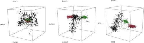
We choose the 0's, 6's and 9's, three hardly classified digits, as an illustration. In this subset of the database, there are 2,219 cases in the training data and 1,035 cases in the test data. We apply the dimension reduction methods to the 16-dimensional predictor vector for the training set, which serves as a preparatory step for the three-group classification problem. Because the response has three slices, SIR estimates only two directions in the dimension reduction subspace. The other methods, SAVE, DCOV and ECD, all estimate three directions. Figure 1 presents the two-dimensional plot of (SIR1, SIR2) and Figure 2 shows the three dimensional plots of (SAVE1, SAVE2, SAVE3), (DCOV1, DCOV2, DCOV3) and (ECD1, ECD2, ECD3). SIR provides only location separation of the three groups. SAVE implies there are covariance differences among three groups, but no clear location separation is provided. Both DCOV and ECD get the location separation and covariance differences, but ECD presents a more clear separation among the three groups.The three-dimensional plot of (ECD1, ECD2, ECD3) gives a comprehensive demonstration of the different features of the three groups.

Figure 1. 2D-plot for the two predictors estimated by SIR.

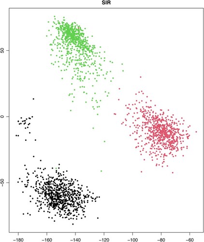
Figure 2. 3D-plots for the three predictors estimated by SAVE, DCOV and ECD.

5. Discussion

In this article, we proposed a new sufficient dimension reduction method. We studied its asymptotic properties and introduced the kNN procedure to estimate the structural dimension d. The numerical studies show that our method can estimate the CS accurately and efficiently. In the future, we consider to develop a variable selection method by combining our method with the penalized method such as LASSO (Tibshirani, 1996). Furthermore, it can be extended to large p small n problems by using the framework of Yin and Hilafu (2015).

Disclosure statement

No potential conflict of interest was reported by the author(s).

Appendix A

Proofs of Propositions 2.1 and 2.2

In order to prove Propositions 2.1 and 2.2 in Section 2.3 in the article, we first provide and prove the following Lemma A.1.

Lemma A.1

Suppose $\eta$ is a basis of the central subspace. Let $({\eta }_1,{\eta }_2)$ be any partition of $\eta$, where ${\eta }^{\mathrm{\top }}{\mathrm{\Sigma }}_{\mathbf{X}}\eta =I_d$. We have ${\mathcal{C}}^2\left({\eta }_i^{\mathrm{\top }}\mathbf{X}|\mathbf{Y}\right)<{\mathcal{C}}^2\left({\eta }^{\mathrm{\top }}\mathbf{X}|\mathbf{Y}\right)$, i = 1, 2.

Proof

Let ${\tilde{\mathbf{X}}}_1={\eta }_1^{\mathrm{\top }}\mathbf{X}$, ${\tilde{\mathbf{X}}}_2={\eta }_2^{\mathrm{\top }}\mathbf{X}$, $F(a,b)={\mathcal{C}}^2\left(\left(\begin{array}{c}a{\tilde{\mathbf{X}}}_1\\ b{\tilde{\mathbf{X}}}_2\end{array}\right)|\mathbf{Y}\right)$, $a\in \mathbb{R}$ and $b\in \mathbb{R}$, and $G_1(a,b)=\mathrm{\partial }F(a,b)/\mathrm{\partial }a$, $G_2(a,b)=\mathrm{\partial }F(a,b)/\mathrm{\partial }b$. A simple calculation shows that $a{G}_1(a,b)+b{G}_2(a,b)=F(a,b)$.

If $({\eta }_1,{\eta }_2)\in \mathcal{S}\left(\eta \right)$, then F(0,1), F(1,0) > 0; otherwise, the conclusion automatically holds.

Claim, if $0\le \lambda <1$, then $F(1,\lambda )<F(1,1)$ and $F(\lambda ,1)<F(1,1)$.

If not, then there exists a $0\le {\lambda }_0<1$ such that $F(1,{\lambda }_0)\ge F(1,1)$ or $F({\lambda }_0,1)\ge F(1,1)$. Without loss of generality, we assume there exists a $0\le {\lambda }_0<1$ such that $F(1,{\lambda }_0)\ge F(1,1)$.

But $F(1,\lambda )=\lambda F(\frac{1}{\lambda },1)$, and as $\lambda \to \mathrm{\infty }$, $F(\frac{1}{\lambda },1)\to F(0,1)>0$. Thus $F(1,\lambda )\to \mathrm{\infty }$, as $\lambda \to \mathrm{\infty }$. That means, there exists a ${\lambda }_1\in ({\lambda }_0,\mathrm{\infty })$ such that $F(1,{\lambda }_1)$ achieves a minimum in $({\lambda }_0,\mathrm{\infty })$. Hence, $G_2(1,{\lambda }_1)=0$. Note that function $F(a,b)$ is a ‘ray’ function, i. e. $F(ca,cb)=cF(a,b)$. Thus using the fact that $F(1,\lambda )=\lambda F(\frac{1}{\lambda },1)$, we can have $G_1(\frac{1}{{\lambda }_1},1)=0$. And it is easy to calculate that $G_1(1,{\lambda }_1)=G_1(\frac{1}{{\lambda }_1},1)=0$.

But $0=1G_1(1,{\lambda }_1)+{\lambda }_1{G}_2(1,{\lambda }_1)=F(1,{\lambda }_1)$. $F(1,{\lambda }_1)=0$ means that $\left(\begin{array}{c}{\tilde{\mathbf{X}}}_1\\ {\lambda }_1{\tilde{\mathbf{X}}}_2\end{array}\right)⫫\mathbf{Y}$, which conflicts with our assumption.

Proof of Proposition 2.1

Since $\mathcal{S}\left(\text{β}\right)\subseteq \mathcal{S}\left(\eta \right)=S_{\mathbf{Y}|\mathbf{X}}$, $d_1\le d$, there exists a matrix $A$, which satisfies $\text{β}=\eta A$. Therefore, ${\mathcal{C}}^2\left({\text{β}}^{\mathrm{\top }}\mathbf{X}|\mathbf{Y}\right)={\mathcal{C}}^2\left(A^{\mathrm{\top }}{\eta }^{\mathrm{\top }}\mathbf{X}|\mathbf{Y}\right)$.

Assume the single value decomposition of A is $U\mathrm{\Sigma }{V}^{\mathrm{\top }}$, where U is a $d\times d$ orthogonal matrix, V is a $d_1\times d_1$ orthogonal matrix and Σ is a $d\times d_1$ diagonal matrix with nonnegative numbers on the diagonal, and it is easy to prove that all nonnegative numbers on the diagonal of Σ are 1. Based on Theorem 3, part (2) of Yin and Yuan (2020), ${\mathcal{C}}^2\left({\text{β}}^{\mathrm{\top }}\mathbf{X}|\mathbf{Y}\right)={\mathcal{C}}^2\left(V{\mathrm{\Sigma }}^{\mathrm{\top }}{U}^{\mathrm{\top }}{\eta }^{\mathrm{\top }}\mathbf{X}|\mathbf{Y}\right)={\mathcal{C}}^2\left({\mathrm{\Sigma }}^{\mathrm{\top }}{U}^{\mathrm{\top }}{\eta }^{\mathrm{\top }}\mathbf{X}|\mathbf{Y}\right)$.

Let $U^{\mathrm{\top }}{\eta }^{\mathrm{\top }}\mathbf{X}=({\tilde{\mathbf{X}}}_1,\dots ,{\tilde{\mathbf{X}}}_d{)}^{\mathrm{\top }}$. Since all nonnegative numbers on the diagonal of Σ are 1 and ${\mathrm{\Sigma }}^{\mathrm{\top }}{U}^{\mathrm{\top }}{\eta }^{\mathrm{\top }}\mathbf{X}=({\tilde{\mathbf{X}}}_1,\dots ,{\tilde{\mathbf{X}}}_{d_1}{)}^{\mathrm{\top }}$, by Lemma A.1, we get ${\mathcal{C}}^2\left({\mathrm{\Sigma }}^{\mathrm{\top }}{U}^{\mathrm{\top }}{\eta }^{\mathrm{\top }}\mathbf{X}|\mathbf{Y}\right)\le {\mathcal{C}}^2\left(U^{\mathrm{\top }}{\eta }^{\mathrm{\top }}\mathbf{X}|\mathbf{Y}\right)$. The equality holds if and only if $d=d_1$. And again based on Theorem 3, part (2) of Yin and Yuan (2020), ${\mathcal{C}}^2\left(U^{\mathrm{\top }}{\eta }^{\mathrm{\top }}\mathbf{X}|\mathbf{Y}\right)={\mathcal{C}}^2\left({\eta }^{\mathrm{\top }}\mathbf{X}|\mathbf{Y}\right)$. Thus, ${\mathcal{C}}^2\left({\text{β}}^{\mathrm{\top }}\mathbf{X}|\mathbf{Y}\right)\le {\mathcal{C}}^2\left({\eta }^{\mathrm{\top }}\mathbf{X}|\mathbf{Y}\right)$, and equality holds if and only if $\mathcal{S}\left(\text{β}\right)=\mathcal{S}\left(\eta \right)$.

Proof of Proposition 2.2

For the $\text{β}$ and $\eta$ described in Proposition 2.2, there exists a rotation matrix $\mathbf{Q}$ such that $\text{β}\mathbf{Q}=({\eta }_a,{\eta }_b)$, and $\mathcal{S}\left({\eta }_a\right)\subseteq \mathcal{S}\left(\eta \right)$, $\mathcal{S}\left({\eta }_b\right)\subseteq \mathcal{S}(\eta {)}^{\mathrm{\perp }}$, where $\mathcal{S}(\eta {)}^{\mathrm{\perp }}$ is the orthogonal space of $\mathcal{S}\left(\eta \right)$.

Since $\mathbf{Y}⫫{\eta }_b^{\mathrm{\top }}\mathbf{X}|{\eta }^{\mathrm{\top }}\mathbf{X}$ and $P_{\eta \left({\mathrm{\Sigma }}_{\mathbf{X}}\right)}^{\mathrm{\top }}\mathbf{X}⫫Q_{\eta \left({\mathrm{\Sigma }}_{\mathbf{X}}\right)}^{\mathrm{\top }}\mathbf{X}$, $\left(\begin{array}{c}\mathbf{Y}\\ {\eta }^{\mathrm{\top }}\mathbf{X}\end{array}\right)⫫{\eta }_b^{\mathrm{\top }}\mathbf{X}$, and according to Proposition 4.3 (Cook, 1998), $\left(\begin{array}{c}\mathbf{Y}\\ {\eta }_a^{\mathrm{\top }}\mathbf{X}\end{array}\right)⫫{\eta }_b^{\mathrm{\top }}\mathbf{X}$. Let $W_1=\left(\begin{array}{c}{\eta }_a^{\mathrm{\top }}\mathbf{X}\\ \mathbf{0}\end{array}\right)$, $V_1=\mathbf{Y}$, $W_2=\left(\begin{array}{c}\mathbf{0}\\ {\eta }_b^{\mathrm{\top }}\mathbf{X}\end{array}\right)$, and $V_2=0$. Then $(W_1,V_1)⫫(W_2,V_2)$. According to Yin and Yuan (2020) Theorem 1, part (2), $\mathcal{C}(W_1+W_2|V_1+V_2)<\mathcal{C}\left(W_1|V_1\right)+\mathcal{C}\left(W_2|V_2\right)$, that is ${\mathcal{C}}^2\left({\mathbf{Q}}^{\mathrm{\top }}{\text{β}}^{\mathrm{\top }}\mathbf{X}|\mathbf{Y}\right)={\mathcal{C}}^2\left({\text{β}}^{\mathrm{\top }}\mathbf{X}|\mathbf{Y}\right)<{\mathcal{C}}^2\left({\eta }_a^{\mathrm{\top }}\mathbf{X}|\mathbf{Y}\right)\le {\mathcal{C}}^2\left({\eta }^{\mathrm{\top }}\mathbf{X}|\mathbf{Y}\right)$.

Appendix B

Proof of Proposition 2.3

In order to prove Proposition 2.3 in Section 2.5 of this article, we provide and prove the following Lemma B.1 first.

Lemma B.1

If the support of X, say S, is compact and furthermore, ${\eta }_n\stackrel{P}{⟶}\eta$, then ${\mathcal{C}}_n^2\left({\eta }_n^{\mathrm{\top }}\mathbf{X}|\mathbf{Y}\right)-{\mathcal{C}}_n^2\left({\eta }^{\mathrm{\top }}\mathbf{X}|\mathbf{Y}\right)\stackrel{P}{⟶}0$.

Proof

Based on Yin and Yuan (2020) Corollary 1, we have that $\begin{array}{rl}& {\mathcal{C}}_n^2\left({\eta }_n^{\mathrm{\top }}\mathbf{X}|\mathbf{Y}\right)=\frac{1}{n^2}\sum _{k,l=1}^{n,n}|{\eta }_n^{\mathrm{\top }}{\mathbf{X}}_k-{\eta }_n^{\mathrm{\top }}{\mathbf{X}}_l|-\frac{1}{n}\sum _{y=1}^H\frac{1}{n_y}\sum _{k,l=1}^{n_y,n_y}|{\eta }_n^{\mathrm{\top }}{\mathbf{X}}_{y,k_y}-{\eta }_n^{\mathrm{\top }}{\mathbf{X}}_{y,l_y}|,\\ & {\mathcal{C}}_n^2\left({\eta }^{\mathrm{\top }}\mathbf{X}|\mathbf{Y}\right)=\frac{1}{n^2}\sum _{k,l=1}^{n,n}|{\eta }^{\mathrm{\top }}{\mathbf{X}}_k-{\eta }^{\mathrm{\top }}{\mathbf{X}}_l|-\frac{1}{n}\sum _{y=1}^H\frac{1}{n_y}\sum _{k,l=1}^{n_y,n_y}|{\eta }^{\mathrm{\top }}{\mathbf{X}}_{y,k_y}-{\eta }^{\mathrm{\top }}{\mathbf{X}}_{y,l_y}|.\end{array}$ Because ${\eta }_n\to \eta$ in probability, let ${\eta }_n=\eta +{ϵ}_n$. Then for any $ϵ>0$, $||{ϵ}_n||<ϵ$, when $n\to \mathrm{\infty }$, where $||\cdot ||$ is the Frobenius norm. Hence, by the condition on X, we have that for a positive constant $c_x$, and large n, $|{\mathcal{C}}_n^2\left({\eta }_n^{\mathrm{\top }}\mathbf{X}|\mathbf{Y}\right)-{\mathcal{C}}_n^2\left({\eta }^{\mathrm{\top }}\mathbf{X}|\mathbf{Y}\right)|\le ϵc_x$. Hence the conclusion follows.

Proof of Proposition 2.3

To simplify the proof, we restrict the support of $\mathbf{X}$ to be a compact set, and it can be shown that ${\mathcal{S}}_{\mathbf{Y}|\mathbf{X}}={\mathcal{S}}_{\mathbf{Y}|{\mathbf{X}}_S}$ (Yin et al., 2008, Proposition 10), where ${\mathbf{X}}_S$ is $\mathbf{X}$ restricted onto S. Without loss of generality, we assume $Q=I_d$. Suppose ${\eta }_n$ is not a consistent estimator of ${\mathcal{S}}_{\mathbf{Y}|\mathbf{X}}$. Then there exists a subsequence, still to be indexed by n, and an ${\eta }^{\ast }$ satisfying ${\eta }^{\ast \mathrm{\top }}{\hat{\mathrm{\Sigma }}}_{\mathbf{X}}{\eta }^{\ast }=I_d$ such that ${\eta }_n\stackrel{P}{⟶}{\eta }^{\ast }$ but $\mathrm{S}\mathrm{p}\mathrm{a}\mathrm{n}\left({\eta }^{\ast }\right)\ne \mathrm{S}\mathrm{p}\mathrm{a}\mathrm{n}\left(\eta \right)$.

By Lemma B.1, we have ${\mathcal{C}}_n^2\left({\eta }_n^{\mathrm{\top }}\mathbf{X}|\mathbf{Y}\right)-{\mathcal{C}}_n^2\left({{\eta }^{\ast }}^{\mathrm{\top }}\mathbf{X}|\mathbf{Y}\right)\stackrel{P}{⟶}0$ and by Lemma 3 in Yin and Yuan (2020), we have ${\mathcal{C}}_n^2({{\eta }^{\ast }}^{\mathrm{\top }}\mathbf{X},\mathbf{Y})\stackrel{\mathrm{a}.\mathrm{s}.}{⟶}{\mathcal{C}}^2\left({{\eta }^{\ast }}^{\mathrm{\top }}X|\mathbf{Y}\right)$. Therefore, ${\mathcal{C}}_n^2\left({\eta }_n^{\mathrm{\top }}\mathbf{X}|\mathbf{Y}\right)\stackrel{P}{⟶}{\mathcal{C}}^2\left({{\eta }^{\ast }}^{\mathrm{\top }}\mathbf{X}|\mathbf{Y}\right)$.

On the other hand, because ${\eta }_n={\arg max}_{{\text{β}}^{\mathrm{\top }}{\hat{\mathrm{\Sigma }}}_{\mathbf{X}}\text{β}=I_d}{\mathcal{C}}_n^2\left({\text{β}}^{\mathrm{\top }}\mathbf{X}|\mathbf{Y}\right)$, we have ${\mathcal{C}}_n^2\left({\eta }_n^{\mathrm{\top }}\mathbf{X}|\mathbf{Y}\right)\ge {\mathcal{C}}_n^2\left({\eta }^{\mathrm{\top }}\mathbf{X}|\mathbf{Y}\right)$. If we take the limit on both sides of the above inequality, we get ${\mathcal{C}}^2\left({{\eta }^{\ast }}^{\mathrm{\top }}\mathbf{X}|\mathbf{Y}\right)\ge {\mathcal{C}}^2\left({\eta }^{\mathrm{\top }}\mathbf{X}|\mathbf{Y}\right)$. However, we have proved that under the assumption $P_{\eta \left({\mathrm{\Sigma }}_{\mathbf{X}}\right)}^{\mathrm{\top }}\mathbf{X}⫫Q_{\eta \left({\mathrm{\Sigma }}_{\mathbf{X}}\right)}^{\mathrm{\top }}\mathbf{X}$, $\eta ={\arg max}_{{\text{β}}^{\mathrm{\top }}{\mathrm{\Sigma }}_{\mathbf{X}}\text{β}=I_d}{\mathcal{C}}^2\left({\text{β}}^{\mathrm{\top }}\mathbf{X}|\mathbf{Y}\right)$, and we also assume that the central subspace is unique. Therefore, ${\mathcal{C}}^2\left({{\eta }^{\ast }}^{\mathrm{\top }}\mathbf{X}|\mathbf{Y}\right)\ge {\mathcal{C}}^2\left({\eta }^{\mathrm{\top }}\mathbf{X}|\mathbf{Y}\right)$ conflicts with the above assumption, so ${\eta }_n$ is a consistent estimator of a basis of the central subspace.

Appendix C

Proof of Proposition 2.4

Lagrange multiplier technique is used to prove the $\sqrt{n}$-consistency of vec$\left({\eta }_n\right)$ in the Proposition 2.4 in Section 2.5 of the article. First, we introduce the following notations and conditions and we also give a new definition.

For a random sample $(\mathbf{X},\mathbf{Y})=\left\{\right({\mathbf{X}}_k,{\mathbf{Y}}_k):k=1,\dots ,n\}$ from the joint distribution of random vectors $\mathbf{X}$ in ${\mathbb{R}}^p$ and $\mathbf{Y}$ in $\mathbb{R}$, let $\mathcal{L}\left(\zeta \right)={\mathcal{C}}^2\left({\text{β}}^{\mathrm{\top }}\mathbf{X}|\mathbf{Y}\right)+{\lambda }^{\mathrm{\top }}\left(\mathrm{v}\mathrm{e}\mathrm{c}\right({\text{β}}^{\mathrm{\top }}{\mathrm{\Sigma }}_{\mathbf{X}}\text{β})-\mathrm{v}\mathrm{e}\mathrm{c}(I_d\left)\right)$ and ${\mathcal{L}}_n\left(\zeta \right)={\mathcal{C}}_n^2\left({\text{β}}^{\mathrm{\top }}\mathbf{X}|\mathbf{Y}\right)+{\lambda }^{\mathrm{\top }}\left(\mathrm{v}\mathrm{e}\mathrm{c}\right({\text{β}}^{\mathrm{\top }}{\hat{\mathrm{\Sigma }}}_{\mathbf{X}}\text{β})-\mathrm{v}\mathrm{e}\mathrm{c}(I_d\left)\right)$. Here $\zeta =\left(\begin{array}{c}\left(\text{β}\right)\\ \lambda \end{array}\right)\in {\mathbb{R}}^{pd+d^2}$, $\text{β}\in {\mathbb{R}}^{p\times d}$, $\lambda \in {\mathbb{R}}^{d^2}$, ${\mathrm{\Sigma }}_{\mathbf{X}}$ is the covariance matrix of X, and ${\hat{\mathrm{\Sigma }}}_{\mathbf{X}}$ is the sample estimate for ${\mathrm{\Sigma }}_{\mathbf{X}}$. Let ${\eta }_n=\arg \underset{{\text{β}}^{\mathrm{\top }}{\hat{\mathrm{\Sigma }}}_{\mathbf{X}}\text{β}=I_d}{max}{\mathcal{C}}_n^2\left({\text{β}}^{\mathrm{\top }}\mathbf{X}|\mathbf{Y}\right)$. Then there exists a ${\lambda }_n$ such that $\left(\begin{array}{c}\mathrm{v}\mathrm{e}\mathrm{c}\left({\eta }_n\right)\\ {\lambda }_n\end{array}\right)$ is a stationary point for ${\mathcal{L}}_n\left(\zeta \right)$. Let ${\theta }_n=\left(\begin{array}{c}\mathrm{v}\mathrm{e}\mathrm{c}\left({\eta }_n\right)\\ {\lambda }_n\end{array}\right)$. Then ${\mathcal{L}}_n^{\mathrm{\prime }}\left({\theta }_n\right)=0$. Let $\eta$ be a basis of CS. Then under the assumption $P_{\eta \left({\mathrm{\Sigma }}_{\mathbf{X}}\right)}^{\mathrm{\top }}\mathbf{X}⫫Q_{\eta \left({\mathrm{\Sigma }}_{\mathbf{X}}\right)}^{\mathrm{\top }}\mathbf{X}$, there exists a rotation matrix $Q:Q^{\mathrm{\top }}Q=I_d$, such that $\eta Q=\arg \underset{{\text{β}}^{\mathrm{\top }}{\mathrm{\Sigma }}_{\mathbf{X}}\text{β}=I_d}{max}{\mathcal{C}}^2\left({\text{β}}^{\mathrm{\top }}\mathbf{X}|\mathbf{Y}\right)$. Without loss of generality, we assume $Q=I_d$ here. Therefore, there exists a ${\lambda }_0$ such that $\left(\begin{array}{c}\mathrm{v}\mathrm{e}\mathrm{c}\left(\eta \right)\\ {\lambda }_0\end{array}\right)$ is a stationary point for $\mathcal{L}\left(\zeta \right)$. Let $\theta =\left(\begin{array}{c}\mathrm{v}\mathrm{e}\mathrm{c}\left(\eta \right)\\ {\lambda }_0\end{array}\right)$.

In the proof, we need to take derivatives of ${\mathcal{C}}^2\left({\eta }^{\mathrm{\top }}\mathbf{X}|\mathbf{Y}\right)$ and ${\mathcal{C}}_n^2\left({\eta }^{\mathrm{\top }}\mathbf{X}|\mathbf{Y}\right)$ with respect to vec$\left(\eta \right)$, so for the simplicity of notation, when we consider the derivatives of ${\mathcal{C}}^2\left({\eta }^{\mathrm{\top }}\mathbf{X}|\mathbf{Y}\right)$ and ${\mathcal{C}}_n^2\left({\eta }^{\mathrm{\top }}\mathbf{X}|\mathbf{Y}\right)$, we use $\mathcal{C}\left(\eta \right)$ and ${\mathcal{C}}_n\left(\eta \right)$ to denote ${\mathcal{C}}^2\left({\eta }^{\mathrm{\top }}\mathbf{X}|\mathbf{Y}\right)$ and ${\mathcal{C}}_n^2\left({\eta }^{\mathrm{\top }}\mathbf{X}|\mathbf{Y}\right)$, respectively.

Here are additional notations, which will be used later in the following proof. $I_{(d,d)}$ is the vec-permutation matrix. $I_m$ is a identity matrix with rank m, and $I_m(:,i)$ denotes the ith column of $I_m$. $\mathbf{A}\otimes \mathbf{B}$ denotes the Kronecker product between matrix $\mathbf{A}$ and $\mathbf{B}$. vec(·) is a vec operator.

Furthermore, we give the following definition and assumptions.

Definition A.1

Let $\mathrm{\Delta }\left(\eta \right)=\{\alpha :||\alpha -\eta ||\le c\}$, where α is a $p\times d$ matrix, ${\alpha }^{\mathrm{\top }}{\mathrm{\Sigma }}_{\mathbf{X}}\alpha =I_d$, c is a fixed small constant, and $||\cdot ||$ is the Frobenius norm. We define an indicator function $\rho (\mathbf{X},{\mathbf{X}}^{\prime })=\{\begin{array}{cc}0,& \text{if}|{\alpha }^{\mathrm{\top }}(\mathbf{X}-{\mathbf{X}}^{\prime })|\le {ϵ}_0,\mathrm{f}\mathrm{o}\mathrm{r}\alpha \in \mathrm{\Delta }\left(\eta \right),\\ 1,& \text{if}|{\alpha }^{\mathrm{\top }}(\mathbf{X}-{\mathbf{X}}^{\prime })|>{ϵ}_0,\mathrm{f}\mathrm{o}\mathrm{r}\alpha \in \mathrm{\Delta }\left(\eta \right),\end{array}$ where ${\mathbf{X}}^{\prime }$ is an i.i.d. copy of $\mathbf{X}$ and ${ϵ}_0$ is a small number. We define the second and third derivatives of $\mathcal{C}\left(\eta \right)$ with respect to vec($\eta$) as ${\mathcal{C}}^{{}^{″}}\left(\eta \right)\rho (\mathbf{X},{\mathbf{X}}^{\prime })$ and ${\mathcal{C}}^{{}^{‴}}\left(\eta \right)\rho (\mathbf{X},{\mathbf{X}}^{\prime })$. For the simplicity of notation, we will still use ${\mathcal{C}}^{{}^{″}}\left(\eta \right)$ and ${\mathcal{C}}^{{}^{‴}}\left(\eta \right)$ to denote ${\mathcal{C}}^{{}^{″}}\left(\eta \right)\rho (\mathbf{X},{\mathbf{X}}^{\prime })$ and ${\mathcal{C}}^{{}^{‴}}\left(\eta \right)\rho (\mathbf{X},{\mathbf{X}}^{\prime })$, respectively.

The reason we use this definition is that under Definition C.1, the second and third derivatives of $\mathcal{C}\left(\eta \right)$ and ${\mathcal{C}}_n\left(\eta \right)$ are bounded, near the neighbourhood of the central subspace.

Assumption C.1

Var$\left[{\varphi }^{\left(1\right)}\right(\mathbf{X},{\mathbf{X}}^{\mathrm{\prime }}\left)\right]$, Var$\left[{\varphi }^{\left(2\mathbf{Y}\right)}\right({\mathbf{X}}_y,{\mathbf{X}}_y^{\mathrm{\prime }}\left)\right],y=1,\dots ,H$, Var$\left[{\varphi }^{\left(3\right)}\right(\mathbf{X}\left)\right]$, Var$\left[{\varphi }^{\left(4\right)}\right((\mathbf{X},{\mathbf{X}}^{\mathrm{\prime }})\left)\right]$, Var$\left[{\varphi }^{\left(5\right)}\right(\mathbf{X}\left)\right]$, Var$\left[{\varphi }^{\left(6\right)}\right((\mathbf{X},{\mathbf{X}}^{\mathrm{\prime }})\left)\right]$, Var$\left[{\varphi }^{\left(7\right)}\right(\mathbf{X}\left)\right]$ are all $<\mathrm{\infty }$. Here $\begin{array}{rl}{\varphi }^{\left(1\right)}(\mathbf{X},{\mathbf{X}}^{\mathrm{\prime }})& =\frac{(I_d\otimes (\mathbf{X}-{\mathbf{X}}^{\mathrm{\prime }}\left)\right)(I_d\otimes (\mathbf{X}-{\mathbf{X}}^{\mathrm{\prime }}{)}^{\mathrm{\top }}\left)\mathrm{v}\mathrm{e}\mathrm{c}\right(\eta )}{|(I_d\otimes (\mathbf{X}-{\mathbf{X}}^{\mathrm{\prime }}{)}^{\mathrm{\top }}\left)\mathrm{v}\mathrm{e}\mathrm{c}\right(\eta )|},\\ {\varphi }^{\left(2y\right)}({\mathbf{X}}_y,{\mathbf{X}}_y^{\mathrm{\prime }})& =\frac{(I_d\otimes ({\mathbf{X}}_y-{\mathbf{X}}_y^{\mathrm{\prime }}\left)\right)(I_d\otimes ({\mathbf{X}}_y-{\mathbf{X}}_y^{\mathrm{\prime }}{)}^{\mathrm{\top }}\left)\mathrm{v}\mathrm{e}\mathrm{c}\right(\eta )}{|(I_d\otimes ({\mathbf{X}}_y-{\mathbf{X}}_y^{\mathrm{\prime }}{)}^{\mathrm{\top }}\left)\mathrm{v}\mathrm{e}\mathrm{c}\right(\eta )|},y=1,\dots ,H,\\ {\varphi }^{\left(3\right)}\left(\mathbf{X}\right)& =(I_d\otimes \mathbf{X}{\mathbf{X}}^{\mathrm{\top }}\eta )(I_{d^2}+I_{d,d}^{\mathrm{\top }}){\lambda }_0,\\ {\varphi }^{\left(4\right)}(\mathbf{X},{\mathbf{X}}^{\mathrm{\prime }})& =\frac{1}{2}(I_d\otimes ({\mathbf{X}{\mathbf{X}}^{\mathrm{\prime }}}^{\mathrm{\top }}+{\mathbf{X}}^{\mathrm{\prime }}{\mathbf{X}}^{\mathrm{\top }}\left)\eta \right)(I_{d^2}+I_{d,d}^{\mathrm{\top }}){\lambda }_0,\\ {\varphi }^{\left(5\right)}\left(\mathbf{X}\right)& =\mathrm{v}\mathrm{e}\mathrm{c}\left({\eta }^{\mathrm{\top }}\mathbf{X}{\mathbf{X}}^{\mathrm{\top }}\eta \right),\\ {\varphi }^{\left(6\right)}(\mathbf{X},{\mathbf{X}}^{\mathrm{\prime }})& =\frac{1}{2}\mathrm{v}\mathrm{e}\mathrm{c}\left({\eta }^{\mathrm{\top }}\right({\mathbf{X}{\mathbf{X}}^{\mathrm{\prime }}}^{\mathrm{\top }}+{\mathbf{X}}^{\mathrm{\prime }}{\mathbf{X}}^{\mathrm{\top }}\left)\eta \right),\\ {\varphi }^{\left(7\right)}\left(\mathbf{X}\right)& =\mathrm{v}\mathrm{e}\mathrm{c}(\mathbf{X}-E\mathbf{X})(\mathbf{X}-E\mathbf{X}{)}^{\mathrm{\top }}.\end{array}$ Here $(\mathbf{X},\mathbf{Y}),({\mathbf{X}}^{\mathrm{\prime }},{\mathbf{Y}}^{\mathrm{\prime }})$ are i.i.d copies and $({\mathbf{X}}_y,{\mathbf{Y}}_y),({\mathbf{X}}_y^{\mathrm{\prime }},{\mathbf{Y}}_y^{\mathrm{\prime }})$ are i.i.d copies in the yth slice.

Assumption C.2

$\left(\begin{array}{cc}{\mathcal{C}}^{{}^{″}}\left(\eta \right)+L& (I_d\otimes {\mathrm{\Sigma }}_{\mathbf{X}}\eta )(I_{d^2}+I_{(d,d)})\\ (I_{d^2}+I_{(d,d)}^{\mathrm{\top }})(I_d\otimes {\eta }^{\mathrm{\top }}{\mathrm{\Sigma }}_{\mathbf{X}})& 0\end{array}\right)$ is nonsingular.

Assumption C.1 is needed for Proposition 2.4 in the main article and Lemma C.1 in the next section, which is similar to the assumed conditions of Theorem 6.1.6 (Lehmann, 1999, Ch. 6). This assumption is required by the asymptotic properties of U-statistics.

Assumption C.2 is in the spirit of von Mises proposition (Serfling, 1980, Section 6.1). In this proposition, it claims that if the first nonvanishing term of Taylor expansion is the linear term, then the $\sqrt{n}$-consistency of the differentiable statistical function can be achieved. In our case, we assume the corresponding matrix is nonsingular, which guarantees the $\sqrt{n}$-consistency. If the matrix is singular, then n or higher order consistency of some parts of our estimates can be proved.

In order to prove Proposition 2.4 in Section 2.5 of the paper, we provide and prove the following Lemma C.1 first.

Lemma C.1

Under Assumptions C.1, C.2 and the assumptions in Proposition 2.4, then $\sqrt{n}({\theta }_n-\theta )\stackrel{\mathcal{D}}{⟶}N(0,\mathbf{V})$. The explicit expression for $\mathbf{V}$ is in the proof.

Proof

The Taylor expansion of ${\mathcal{L}}_n^{\mathrm{\prime }}\left({\theta }_n\right)$ at $\theta$ is $0={\mathcal{L}}_n^{\mathrm{\prime }}\left({\theta }_n\right)={\mathcal{L}}_n^{\mathrm{\prime }}\left(\theta \right)+{\mathcal{L}}_n^{{}^{″}}\left(\theta \right)({\theta }_n-\theta )+{\mathcal{R}}_1\left({\theta }_n^{\ast }\right)$, where $||{\theta }_n^{\ast }-\theta ||\le ||{\theta }_n-\theta ||$, where $||\cdot ||$ is the Frobenius norm and ${\theta }_n^{\ast }=\left(\begin{array}{c}\mathrm{v}\mathrm{e}\mathrm{c}\left({\eta }_n^{\ast }\right)\\ {\lambda }_n^{\ast }\end{array}\right)$. Next, we will give explicit expressions of ${\mathcal{L}}_n^{\mathrm{\prime }}\left(\theta \right)$, ${\mathcal{L}}_n^{{}^{″}}\left(\theta \right)$ and ${\mathcal{R}}_1\left({\theta }_n^{\ast }\right)$. With simple calculation, ${\mathcal{L}}_n^{\mathrm{\prime }}\left(\theta \right)=\left(\begin{array}{c}{\mathcal{C}}_n^{\mathrm{\prime }}\left(\eta \right)+(I_d\otimes {\hat{\mathrm{\Sigma }}}_{\mathbf{X}}\eta )(I_{d^2}+I_{(d,d)}){\lambda }_0\mathrm{v}\mathrm{e}\mathrm{c}\left({\eta }^{\mathrm{\top }}{\hat{\mathrm{\Sigma }}}_{\mathbf{X}}\eta \right)-\mathrm{v}\mathrm{e}\mathrm{c}\left(I_d\right)\end{array}\right)$, ${\mathcal{L}}_n^{{}^{″}}\left(\theta \right)=\left(\begin{array}{cc}{\mathcal{C}}_n^{{}^{″}}\left(\eta \right)+\hat{L}& (I_d\otimes {\hat{\mathrm{\Sigma }}}_{\mathbf{X}}\eta )(I_{d^2}+I_{(d,d)})\\ (I_{d^2}+I_{(d,d)}^{\mathrm{\top }})(I_d\otimes {\eta }^{\mathrm{\top }}{\hat{\mathrm{\Sigma }}}_{\mathbf{X}})& 0\end{array}\right),$ where $\hat{L}=\left(\mathrm{v}\mathrm{e}\mathrm{c}\right({\hat{L}}_{11}),\mathrm{v}\mathrm{e}\mathrm{c}({\hat{L}}_{21}),\dots ,\mathrm{v}\mathrm{e}\mathrm{c}({\hat{L}}_{p1}),\dots ,\mathrm{v}\mathrm{e}\mathrm{c}({\hat{L}}_{1d}),\mathrm{v}\mathrm{e}\mathrm{c}({\hat{L}}_{2d}),\dots ,\mathrm{v}\mathrm{e}\mathrm{c}({\hat{L}}_{pd}){)}^{\mathrm{\top }}$ and ${\hat{L}}_{ij}={\hat{\mathrm{\Sigma }}}_{\mathbf{X}}^{\mathrm{\top }}{I}_p(:,i){\lambda }_0^{\mathrm{\top }}(I_{d^2}+I_{(d,d)}^{\mathrm{\top }})\left(I_d\right(:,j)\otimes I_d).$ It is obvious that $\hat{L}\stackrel{\mathrm{a}.\mathrm{s}.}{⟶}L$, where $L=\left(\mathrm{v}\mathrm{e}\mathrm{c}\right(L_{11}),\mathrm{v}\mathrm{e}\mathrm{c}(L_{21}),\dots ,\mathrm{v}\mathrm{e}\mathrm{c}(L_{p1}),\dots ,\mathrm{v}\mathrm{e}\mathrm{c}(L_{1d}),\mathrm{v}\mathrm{e}\mathrm{c}(L_{2d}),\dots ,\mathrm{v}\mathrm{e}\mathrm{c}(L_{pd}){)}^{\mathrm{\top }}$ and $L_{ij}={\mathrm{\Sigma }}_X^{\mathrm{\top }}{I}_p(:,i){\lambda }_0^{\mathrm{\top }}(I_{d^2}+I_{(d,d)}^{\mathrm{\top }})\left(I_d\right(:,j)\otimes I_d).$ Here $i=1,\dots ,p$ and $j=1,\dots ,d.$

The remainder term ${\mathcal{R}}_1\left({\theta }_n^{\ast }\right)$ involves the third derivative of $\mathcal{L}\left(\zeta \right)$ at ${\theta }_n^{\ast }$. Let $T_n={\mathcal{L}}_n^{{}^{‴}}\left({\theta }_n^{\ast }\right)$, where $T_n$ is a $(pd+d^2)\times (pd+d^2)\times (pd+d^2)$ array and each $T_n(j,:,:),j=1,\dots ,pd+d^2$, is a $(pd+d^2)\times (pd+d^2)$ matrix. Therefore, the form of ${\mathcal{R}}_1\left({\theta }_n^{\ast }\right)$ can be written as ${\mathcal{R}}_1\left({\theta }_n^{\ast }\right)=\frac{1}{2}\left(\begin{array}{c}({\theta }_n-\theta {)}^{\mathrm{\top }}{T}_n(1,:,:\left)\right({\theta }_n-\theta )\\ ({\theta }_n-\theta {)}^{\mathrm{\top }}{T}_n(2,:,:\left)\right({\theta }_n-\theta )\\ ⋮\\ ({\theta }_n-\theta {)}^{\mathrm{\top }}{T}_n(pd+d^2,:,:\left)\right({\theta }_n-\theta )\end{array}\right).$ Based on the above explicit expression of ${\mathcal{L}}_n^{\mathrm{\prime }}\left(\theta \right)$, ${\mathcal{L}}_n^{{}^{″}}\left(\theta \right)$ and ${\mathcal{R}}_1\left({\theta }_n^{\ast }\right)$, the Taylor expansion of ${\mathcal{L}}_n^{\mathrm{\prime }}\left({\theta }_n\right)$ at $\theta$ can be written as $\begin{array}{rl}0& =\left(\begin{array}{c}{\mathcal{C}}_n^{\prime }\left(\mathit{\eta }\right)+(I_d\otimes {\hat{\mathrm{\Sigma }}}_{\mathbf{X}}\mathit{\eta })(I_{d^2}+I_{(d,d)}{\lambda }_0)\\ \mathrm{v}\mathrm{e}\mathrm{c}\left({\mathit{\eta }}^{\mathrm{\top }}{\hat{\mathrm{\Sigma }}}_{\mathbf{X}}\mathit{\eta }\right)-\mathrm{v}\mathrm{e}\mathrm{c}\left(I_d\right)\end{array}\right)\\ & +\left(\begin{array}{cc}{\mathcal{C}}_n^{″}\left(\mathit{\eta }\right)+\hat{L}& (I_d\otimes {\hat{\mathrm{\Sigma }}}_{\mathbf{X}}\mathit{\eta })(I_{d^2}+I_{(d,d)})\\ (I_{d^2}+I_{(d,d)}^{\mathrm{\top }})(I_d\otimes {\mathit{\eta }}^{\mathrm{\top }}{\hat{\mathrm{\Sigma }}}_{\mathbf{X}}\mathit{\eta })& 0\end{array}\right)({\mathit{\theta }}_n-\mathit{\theta })\\ & +\frac{1}{2}\left(\begin{array}{c}({\mathit{\theta }}_n-\mathit{\theta }{)}^{\mathrm{\top }}{T}_n(1,:,:\left)\right({\mathit{\theta }}_n-\mathit{\theta })\\ ({\mathit{\theta }}_n-\mathit{\theta }{)}^{\mathrm{\top }}{T}_n(2,:,:\left)\right({\mathit{\theta }}_n-\mathit{\theta })\\ ⋮\\ ({\mathit{\theta }}_n-\mathit{\theta }{)}^{\mathrm{\top }}{T}_n(pd+d^2,:,:\left)\right({\mathit{\theta }}_n-\mathit{\theta })\end{array}\right).\end{array}$ From the above Taylor expansion of ${\mathcal{L}}_n^{\mathrm{\prime }}\left({\theta }_n\right)$ at $\theta$, we get $\begin{array}{rl}& -{\left(\begin{array}{cc}{\mathcal{C}}_n^{″}\left(\mathit{\eta }\right)+\hat{L}& (I_d\otimes {\hat{\mathrm{\Sigma }}}_{\mathbf{X}}\mathit{\eta })(I_{d^2}+I_{(d,d)})\\ (I_{d^2}+I_{(d,d)}^{\mathrm{\top }})(I_d\otimes {\mathit{\eta }}^{\mathrm{\top }}{\hat{\mathrm{\Sigma }}}_{\mathbf{X}}\mathit{\eta })& 0\end{array}\right)}^{-1}\\ & \times \sqrt{n}\left(\begin{array}{c}{\mathcal{C}}_n^{\prime }\left(\mathit{\eta }\right)+(I_d\otimes {\hat{\mathrm{\Sigma }}}_{\mathbf{X}}\mathit{\eta })(I_{d^2}+I_{(d,d)}{\lambda }_0)\\ \mathrm{v}\mathrm{e}\mathrm{c}\left({\mathit{\eta }}^{\mathrm{\top }}{\hat{\mathrm{\Sigma }}}_{\mathbf{X}}\mathit{\eta }\right)-\mathrm{v}\mathrm{e}\mathrm{c}\left(I_d\right)\end{array}\right)\\ & =[I_{pd+d^2}+\frac{1}{2}{\left(\begin{array}{cc}{\mathcal{C}}_n^{″}\left(\mathit{\eta }\right)+\hat{L}& (I_d\otimes {\hat{\mathrm{\Sigma }}}_{\mathbf{X}}\mathit{\eta })(I_{d^2}+I_{(d,d)})\\ (I_{d^2}+I_{(d,d)}^{\mathrm{\top }})(I_d\otimes {\mathit{\eta }}^{\mathrm{\top }}{\hat{\mathrm{\Sigma }}}_{\mathbf{X}}\mathit{\eta })& 0\end{array}\right)}^{-1}\\ & \times \left(\begin{array}{c}({\mathit{\theta }}_n-\theta {)}^{\mathrm{\top }}{T}_n(1,:,:)\\ ({\mathit{\theta }}_n-\theta {)}^{\mathrm{\top }}{T}_n(2,:,:)\\ ⋮\\ ({\mathit{\theta }}_n-\theta {)}^{\mathrm{\top }}{T}_n(pd+d^2,:,:)\end{array}\right)]\sqrt{n}({\mathit{\theta }}_n-\theta ).\end{array}$ Next, we will prove two parts.

Part 1: $\begin{array}{rl}& -{\left(\begin{array}{cc}{\mathcal{C}}_n^{{}^{″}}\left(\eta \right)+\hat{L}& (I_d\otimes {\hat{\mathrm{\Sigma }}}_{\mathbf{X}}\eta )(I_{d^2}+I_{(d,d)})\\ (I_{d^2}+I_{(d,d)}^{\mathrm{\top }})(I_d\otimes {\eta }^{\mathrm{\top }}{\hat{\mathrm{\Sigma }}}_{\mathbf{X}})& 0\end{array}\right)}^{-1}\\ & \times \sqrt{n}\left(\begin{array}{c}{\mathcal{C}}_n^{\mathrm{\prime }}\left(\eta \right)+(I_d\otimes {\hat{\mathrm{\Sigma }}}_{\mathbf{X}}\eta )(I_{d^2}+I_{(d,d)}){\lambda }_0\\ \$vec\$\left({\eta }^{\mathrm{\top }}{\hat{\mathrm{\Sigma }}}_{\mathbf{X}}\eta \right)-\$vec\$\left(I_d\right)\end{array}\right)⟶N(0,\mathbf{V}).\end{array}$

Part 2: $\begin{array}{rl}\sqrt{n}({\theta }_n-\theta )& \stackrel{\mathcal{D}}{=}[I_{pd+d^2}+\frac{1}{2}{\left(\begin{array}{cc}{\mathcal{C}}_n^{{}^{″}}\left(\eta \right)+\hat{L}& (I_d\otimes {\hat{\mathrm{\Sigma }}}_{\mathbf{X}}\eta )(I_{d^2}+I_{(d,d)})\\ (I_{d^2}+I_{(d,d)}^{\mathrm{\top }})(I_d\otimes {\eta }^{\mathrm{\top }}{\hat{\mathrm{\Sigma }}}_{\mathbf{X}})& 0\end{array}\right)}^{-1}\\ & \times \left(\begin{array}{c}({\theta }_n-\theta {)}^{\mathrm{\top }}{T}_n(1,:,:)\\ ({\theta }_n-\theta {)}^{\mathrm{\top }}{T}_n(2,:,:)\\ ⋮\\ ({\theta }_n-\theta {)}^{\mathrm{\top }}{T}_n(pd+d^2,:,:)\end{array}\right)]\sqrt{n}({\theta }_n-\theta ).\end{array}$

Proof of part 1

We will show that both ${\mathcal{C}}_n^{\mathrm{\prime }}\left(\eta \right)+(I_d\otimes {\hat{\mathrm{\Sigma }}}_{\mathbf{X}}\eta )(I_{d^2}+I_{(d,d)}){\lambda }_0$ and vec$\left({\eta }^{\mathrm{\top }}{\hat{\mathrm{\Sigma }}}_{\mathbf{X}}\eta \right)-\mathrm{v}\mathrm{e}\mathrm{c}\left(I_d\right)$ are linear combinations of U-statistics and the asymptotic distribution can be achieved by the asymptotic property of U-statistics.

Based on Corollary 1 in Yin and Yuan (2020), ${\mathcal{C}}_n\left(\eta \right)=\frac{1}{n^2}\sum _{k,l=1}^{n,n}|{\eta }^{\mathrm{\top }}({\mathbf{X}}_k-{\mathbf{X}}_l)|-\frac{1}{n}\sum _{y=1}^H\frac{1}{n_y}\sum _{k,l=1}^{n_y,n_y}|{\eta }^{\mathrm{\top }}({\mathbf{X}}_{y,k_y}-{\mathbf{X}}_{y,l_y})|.$ With some calculation, we can get ${\mathcal{C}}_n^{\mathrm{\prime }}\left(\eta \right)+(I_d\otimes {\hat{\mathrm{\Sigma }}}_{\mathbf{X}}\eta )(I_{d^2}+I_{(d,d)}){\lambda }_0=\frac{n-1}{n}{\mathbf{U}}_{1n}-\frac{1}{n}\sum _{y=1}^H(n_y-1){\mathbf{U}}_{2y}+\frac{n-1}{n}{\mathbf{U}}_{3n}-\frac{n-1}{n}{\mathbf{U}}_{4n},$ where $\begin{array}{rl}{\mathbf{U}}_{1n}& ={(\genfrac{}{}{0ex}{}{n}{2})}^{-1}\sum _{1\le k<l\le n}\frac{(I_d\otimes ({\mathbf{X}}_k-{\mathbf{X}}_l\left)\right)(I_d\otimes ({\mathbf{X}}_k-{\mathbf{X}}_l{)}^{\mathrm{\top }}\left)\mathrm{v}\mathrm{e}\mathrm{c}\right(\eta )}{|(I_d\otimes ({\mathbf{X}}_k-{\mathbf{X}}_l{)}^{\mathrm{\top }}\left)\mathrm{v}\mathrm{e}\mathrm{c}\right(\eta )|},\\ {\mathbf{U}}_{2y}& ={(\genfrac{}{}{0ex}{}{n_y}{2})}^{-1}\sum _{1\le k_y<l_y\le n_y}\frac{(I_d\otimes ({\mathbf{X}}_{y,k_y}-{\mathbf{X}}_{y,l_y}\left)\right)(I_d\otimes ({\mathbf{X}}_{y,k_y}-{\mathbf{X}}_{y,l_y}{)}^{\mathrm{\top }}\left)\mathrm{v}\mathrm{e}\mathrm{c}\right(\eta )}{|(I_d\otimes ({\mathbf{X}}_{y,k_y}-{\mathbf{X}}_{y,l_y}{)}^{\mathrm{\top }}\left)\mathrm{v}\mathrm{e}\mathrm{c}\right(\eta )|},y=1,\dots ,H,\\ {\mathbf{U}}_{3n}& =\frac{1}{n}\sum _{i=1}^n(I_d\otimes {\mathbf{X}}_i{\mathbf{X}}_i^{\mathrm{\top }}\eta )(I_{d^2}+I_{d,d}^{\mathrm{\top }}){\lambda }_0,\\ {\mathbf{U}}_{4n}& ={(\genfrac{}{}{0ex}{}{n}{2})}^{-1}\sum _{i<j}\frac{1}{2}(I_d\otimes ({\mathbf{X}}_i{\mathbf{X}}_j^{\mathrm{\top }}+{\mathbf{X}}_j{\mathbf{X}}_i^{\mathrm{\top }}\left)\eta \right)(I_{d^2}+I_{d,d}^{\mathrm{\top }}){\lambda }_0.\end{array}$ Here ${\mathbf{U}}_{1n}$, ${\mathbf{U}}_{2y}(y=1,\dots ,H)$, ${\mathbf{U}}_{3n}$, ${\mathbf{U}}_{4n}$ are U-statistics. In the notation ${\mathbf{U}}_{2y}$, $y=1,\dots ,H$, $k_y,l_y=1,\dots ,n_y$, where H denotes the number of slices and $n_y$ is the number of samples in the yth slice.

Considering the term vec$\left({\eta }^{\mathrm{\top }}{\hat{\mathrm{\Sigma }}}_{\mathbf{X}}\eta \right)$, which is also a linear combination of U-statistics, let $\begin{array}{rl}{\mathbf{U}}_{5n}& =\frac{1}{n}\sum _{i=1}^n\mathrm{v}\mathrm{e}\mathrm{c}\left({\eta }^{\mathrm{\top }}{\mathbf{X}}_i{\mathbf{X}}_i^{\mathrm{\top }}\eta \right),\\ {\mathbf{U}}_{6n}& ={(\genfrac{}{}{0ex}{}{n}{2})}^{-1}\sum _{i<j}\frac{1}{2}\mathrm{v}\mathrm{e}\mathrm{c}\left({\eta }^{\mathrm{\top }}\right({\mathbf{X}}_i{\mathbf{X}}_j^{\mathrm{\top }}+{\mathbf{X}}_j{\mathbf{X}}_i^{\mathrm{\top }}\left)\eta \right),\end{array}$ and then vec$\left({\eta }^{\mathrm{\top }}{\hat{\mathrm{\Sigma }}}_{\mathbf{X}}\eta \right)=\frac{n-1}{n}{\mathbf{U}}_{5n}-\frac{n-1}{n}{\mathbf{U}}_{6n}$.

Let $\begin{array}{rl}{\mu }_1& =E\frac{(I_d\otimes (\mathbf{X}-{\mathbf{X}}^{\mathrm{\prime }}\left)\right)(I_d\otimes (\mathbf{X}-{\mathbf{X}}^{\mathrm{\prime }}{)}^{\mathrm{\top }}\left)\mathrm{v}\mathrm{e}\mathrm{c}\right(\eta )}{|(I_d\otimes (\mathbf{X}-{\mathbf{X}}^{\mathrm{\prime }}{)}^{\mathrm{\top }}\left)\mathrm{v}\mathrm{e}\mathrm{c}\right(\eta )|},\\ {\mu }_{2y}& =E\frac{(I_d\otimes ({\mathbf{X}}_y-{\mathbf{X}}_y^{\mathrm{\prime }}\left)\right)(I_d\otimes ({\mathbf{X}}_y-{\mathbf{X}}_y^{\mathrm{\prime }}{)}^{\mathrm{\top }}\left)\mathrm{v}\mathrm{e}\mathrm{c}\right(\eta )}{|(I_d\otimes ({\mathbf{X}}_y-{\mathbf{X}}_y^{\mathrm{\prime }}{)}^{\mathrm{\top }}\left)\mathrm{v}\mathrm{e}\mathrm{c}\right(\eta )|},y=1,\dots ,H,\\ {\mu }_3& =E(I_d\otimes \mathbf{X}{\mathbf{X}}^{\mathrm{\top }}\eta )(I_{d^2}+I_{(d,d)}^{\mathrm{\top }}){\lambda }_0,\\ {\mu }_4& =(I_d\otimes (E\mathbf{X}\left)\right(E\mathbf{X}{)}^{\mathrm{\top }}\eta \left)\right(I_{d^2}+I_{(d,d)}^{\mathrm{\top }}){\lambda }_0,\\ {\mu }_5& =\mathrm{v}\mathrm{e}\mathrm{c}\left({\eta }^{\mathrm{\top }}\right(E\mathbf{X}{\mathbf{X}}^{\mathrm{\top }}\left)\eta \right),\\ {\mu }_6& =\mathrm{v}\mathrm{e}\mathrm{c}\left({\eta }^{\mathrm{\top }}\right(E\mathbf{X}\left)\right(E\mathbf{X}{)}^{\mathrm{\top }}\eta ).\end{array}$ Here $(\mathbf{X},\mathbf{Y}),({\mathbf{X}}^{\mathrm{\prime }},{\mathbf{Y}}^{\mathrm{\prime }})$ are i.i.d copies and $({\mathbf{X}}_y,{\mathbf{Y}}_y)({\mathbf{X}}_y^{\mathrm{\prime }},{\mathbf{Y}}_y^{\mathrm{\prime }})$ are i.i.d copies in the yth slice.

According to Theorem 6.1.6 (Lehmann, 1999, Ch.6), $\sqrt{n}\left(\begin{array}{c}{\mathbf{U}}_{1n}-{\mu }_1\\ {\mathbf{U}}_{21}-{\mu }_{21}\\ ⋮\\ {\mathbf{U}}_{2H}-{\mu }_{2H}\\ {\mathbf{U}}_{3n}-{\mu }_3\\ {\mathbf{U}}_{4n}-{\mu }_4\\ {\mathbf{U}}_{5n}-{\mu }_5\\ {\mathbf{U}}_{6n}-{\mu }_6\end{array}\right)\stackrel{\mathcal{D}}{⟶}N(0,\mathrm{\Sigma }),$ where $\mathrm{\Sigma }=\left(\begin{array}{ccc}{\mathrm{\Sigma }}_{11}& \cdots & {\mathrm{\Sigma }}_{1(H+5)}\\ ⋮& \ddots & ⋮\\ {\mathrm{\Sigma }}_{(H+5)1}& \cdots & {\mathrm{\Sigma }}_{(H+5)(H+5)}\end{array}\right).$

Let $\mathbf{B}=\left(\begin{array}{cccccccc}{I}_{pd}& (-\frac{1}{H})I_{pd}& \cdots & (-\frac{1}{H})I_{pd}& I_{pd}& -I_{pd}& \mathbf{0}& \mathbf{0}\\ {\mathbf{0}}^{\mathrm{\top }}& {\mathbf{0}}^{\mathrm{\top }}& \cdots & {\mathbf{0}}^{\mathrm{\top }}& {\mathbf{0}}^{\mathrm{\top }}& {\mathbf{0}}^{\mathrm{\top }}& I_{d^2\times d^2}& -I_{d^2\times d^2}\end{array}\right)$, where $\mathbf{0}$ is a $pd\times d^2$ zero matrix. Then $\sqrt{n}\mathbf{B}\left(\begin{array}{c}{\mathbf{U}}_{1n}-{\mu }_1\\ {\mathbf{U}}_{21}-{\mu }_{21}\\ ⋮\\ {\mathbf{U}}_{2H}-{\mu }_{2H}\\ {\mathbf{U}}_{3n}-{\mu }_3\\ {\mathbf{U}}_{4n}-{\mu }_4\\ {\mathbf{U}}_{5n}-{\mu }_5\\ {\mathbf{U}}_{6n}-{\mu }_6\end{array}\right)=\sqrt{n}\left(\begin{array}{c}{\mathbf{U}}_{1n}-\frac{1}{H}\sum _{y=1}^H{\mathbf{U}}_{2y}+{\mathbf{U}}_{3n}-{\mathbf{U}}_{4n}\\ {\mathbf{U}}_{5n}-{\mathbf{U}}_{6n}-\mathrm{v}\mathrm{e}\mathrm{c}\left(I_d\right)\end{array}\right).$

Note that $$\begin{gathered} \sqrt{n}\left(\begin{array}{c}{\mathcal{C}}_n^{\mathrm{\prime }}\left(\eta \right)+(I_d\otimes {\hat{\mathrm{\Sigma }}}_{\mathbf{X}}\eta )(I_{d^2}+I_{(d,d)}){\lambda }_0\\ \mathrm{v}\mathrm{e}\mathrm{c}\left({\eta }^{\mathrm{\top }}{\hat{\mathrm{\Sigma }}}_{\mathbf{X}}\eta \right)-\mathrm{v}\mathrm{e}\mathrm{c}\left(I_d\right)\end{array}\right)= \\ \sqrt{n}\left(\begin{array}{c}\frac{n-1}{n}{\mathbf{U}}_{1n}-\frac{1}{n}\sum _{y=1}^H(n_y-1){\mathbf{U}}_{2y}+\frac{n-1}{n}{\mathbf{U}}_{3n}-\frac{n-1}{n}{\mathbf{U}}_{4n}\\ \frac{n-1}{n}{\mathbf{U}}_{5n}-\frac{n-1}{n}{\mathbf{U}}_{6n}-\mathrm{v}\mathrm{e}\mathrm{c}\left(I_d\right)\end{array}\right), \end{gathered}$$ and under Assumption C.1, $\begin{array}{rl}& \sqrt{n}\left(\begin{array}{c}\frac{(n-1)}{n}{\mathbf{U}}_{1n}-\frac{1}{n}\sum _{y=1}^H(n_y-1){\mathbf{U}}_{2y}+\frac{n-1}{n}{\mathbf{U}}_{3n}-\frac{n-1}{n}{\mathbf{U}}_{4n}\\ \frac{n-1}{n}{\mathbf{U}}_{5n}-\frac{n-1}{n}{\mathbf{U}}_{6n}-\mathrm{v}\mathrm{e}\mathrm{c}\left(I_d\right)\end{array}\right)\\ & -\sqrt{n}\left(\begin{array}{c}{\mathbf{U}}_{1n}-\frac{1}{H}\sum _{y=1}^H{\mathbf{U}}_{2y}+{\mathbf{U}}_{3n}+{\mathbf{U}}_{4n}\\ {\mathbf{U}}_{5n}-{\mathbf{U}}_{6n}-\mathrm{v}\mathrm{e}\mathrm{c}\left(I_d\right)\end{array}\right)\stackrel{P}{⟶}0.\end{array}$ Therefore, according to Slutsky's theorem, $\begin{array}{r}\sqrt{n}\left(\begin{array}{c}{\mathcal{C}}_n^{\mathrm{\prime }}\left(\eta \right)+(I_d\otimes {\hat{\mathrm{\Sigma }}}_{\mathbf{X}}\eta )(I_{d^2}+I_{(d,d)}){\lambda }_0\\ \mathrm{v}\mathrm{e}\mathrm{c}\left({\eta }^{\mathrm{\top }}{\hat{\mathrm{\Sigma }}}_{\mathbf{X}}\eta \right)-\mathrm{v}\mathrm{e}\mathrm{c}\left(I_d\right)\end{array}\right)\stackrel{D}{=}\sqrt{n}\mathbf{B}\left(\begin{array}{c}{\mathbf{U}}_{1n}-{\mu }_1\\ {\mathbf{U}}_{21}-{\mu }_{21}\\ ⋮\\ {\mathbf{U}}_{2H}-{\mu }_{2H}\\ {\mathbf{U}}_{3n}-{\mu }_3\\ {\mathbf{U}}_{4n}-{\mu }_4\\ {\mathbf{U}}_{5n}-{\mu }_5\\ {\mathbf{U}}_{6n}-{\mu }_6\end{array}\right).\end{array}$

Let $\begin{array}{rl}{A}_n& ={\left(\begin{array}{cc}{\mathcal{C}}_n^{{}^{″}}\left(\eta \right)+\hat{L}& (I_d\otimes {\hat{\mathrm{\Sigma }}}_{\mathbf{X}}\eta )(I_{d^2}+I_{(d,d)})\\ (I_{d^2}+I_{(d,d)}^{\mathrm{\top }})(I_d\otimes {\eta }^{\mathrm{\top }}{\hat{\mathrm{\Sigma }}}_{\mathbf{X}})& 0\end{array}\right)}^{-1},\\ A& ={\left(\begin{array}{cc}{\mathcal{C}}^{{}^{″}}\left(\eta \right)+L& (I_d\otimes {\mathrm{\Sigma }}_{\mathbf{X}}\eta )(I_{d^2}+I_{(d,d)})\\ (I_{d^2}+I_{(d,d)}^{\mathrm{\top }})(I_d\otimes {\eta }^{\mathrm{\top }}{\mathrm{\Sigma }}_{\mathbf{X}})& 0\end{array}\right)}^{-1}.\end{array}$

Under Assumption C.2 and our definition of second derivative of ${\mathcal{C}}_n\left(\eta \right)$, by SLLN of U-statistics, $A_n\stackrel{\mathrm{a}.\mathrm{s}.}{⟶}A$. Therefore, $\begin{array}{rl}& {\left(\begin{array}{cc}{\mathcal{C}}_n^{{}^{″}}\left(\eta \right)+\hat{L}& (I_d\otimes {\hat{\mathrm{\Sigma }}}_{\mathbf{X}}\eta )(I_{d^2}+I_{(d,d)})\\ (I_{d^2}+I_{(d,d)}^{\mathrm{\top }})(I_d\otimes {\eta }^{\mathrm{\top }}{\hat{\mathrm{\Sigma }}}_{\mathbf{X}})& 0\end{array}\right)}^{-1}\\ & \times \sqrt{n}\left(\begin{array}{c}{\mathcal{C}}_n^{\mathrm{\prime }}\left(\eta \right)+(I_d\otimes {\hat{\mathrm{\Sigma }}}_{\mathbf{X}}\eta )(I_{d^2}+I_{(d,d)}){\lambda }_0\\ \mathrm{v}\mathrm{e}\mathrm{c}\left({\eta }^{\mathrm{\top }}{\hat{\mathrm{\Sigma }}}_{\mathbf{X}}\eta \right)-\mathrm{v}\mathrm{e}\mathrm{c}\left(I_d\right)\end{array}\right)\stackrel{D}{=}\sqrt{n}\mathbf{A}\mathbf{B}\left(\begin{array}{c}{\mathbf{U}}_{1n}-{\mu }_1\\ {\mathbf{U}}_{21}-{\mu }_{21}\\ ⋮\\ {\mathbf{U}}_{2H}-{\mu }_{2H}\\ {\mathbf{U}}_{3n}-{\mu }_3\\ {\mathbf{U}}_{4n}-{\mu }_4\\ {\mathbf{U}}_{5n}-{\mu }_5\\ {\mathbf{U}}_{6n}-{\mu }_6\end{array}\right)⟶N(0,\mathbf{V}),\end{array}$ where $\mathbf{V}=\mathbf{A}\mathbf{B}\mathrm{\Sigma }{\mathbf{B}}^{\mathrm{\top }}{\mathbf{A}}^{\mathrm{\top }}$.

Proof of part 2

Under Assumption C.2 and Definition C.1, $$\begin{gathered} I_{pd+d^2}+\frac{1}{2}{\left(\begin{array}{cc}{\mathcal{C}}_n^{{}^{″}}\left(\eta \right)+\hat{L}& (I_d\otimes {\hat{\mathrm{\Sigma }}}_{\mathbf{X}}\eta )(I_{d^2}+I_{(d,d)})\\ (I_{d^2}+I_{(d,d)}^{\mathrm{\top }})(I_d\otimes {\eta }^{\mathrm{\top }}{\hat{\mathrm{\Sigma }}}_{\mathbf{X}})& 0\end{array}\right)}^{-1}\left(\begin{array}{c}({\theta }_n-\theta {)}^{\mathrm{\top }}{T}_n(1,:,:)\\ ({\theta }_n-\theta {)}^{\mathrm{\top }}{T}_n(2,:,:)\\ ⋮\\ ({\theta }_n-\theta {)}^{\mathrm{\top }}{T}_n(pd+d^2,:,:)\end{array}\right) \\ \stackrel{P}{⟶}{I}_{pd+d^2}. \end{gathered}$$ Therefore, by Slutsky's theorem, $\begin{array}{rl}\sqrt{n}({\theta }_n-\theta )& \stackrel{\mathcal{D}}{=}[I_{pd+d^2}+\frac{1}{2}{\left(\begin{array}{cc}{\mathcal{C}}_n^{{}^{″}}\left(\eta \right)+\left(\begin{array}{c}{\mathrm{v}\mathrm{e}\mathrm{c}}^{\mathrm{\top }}\left({\hat{L}}_{11}\right)\\ ⋮\\ {\mathrm{v}\mathrm{e}\mathrm{c}}^{\mathrm{\top }}\left({\hat{L}}_{pd}\right)\end{array}\right)& (I_d\otimes {\hat{\mathrm{\Sigma }}}_{\mathbf{X}}\eta )(I_{d^2}+I_{(d,d)})\\ (I_{d^2}+I_{(d,d)}^{\mathrm{\top }})(I_d\otimes {\eta }^{\mathrm{\top }}{\hat{\mathrm{\Sigma }}}_{\mathbf{X}})& 0\end{array}\right)}^{-1}\left(\begin{array}{c}({\theta }_n-\theta {)}^{\mathrm{\top }}{T}_n(1,:,:)\\ ({\theta }_n-\theta {)}^{\mathrm{\top }}{T}_n(2,:,:)\\ ⋮\\ ({\theta }_n-\theta {)}^{\mathrm{\top }}{T}_n(pd+d^2,:,:)\end{array}\right)]\\ & \times \sqrt{n}({\theta }_n-\theta ).\end{array}$ Therefore, $\sqrt{n}({\theta }_n-\theta )\stackrel{\mathcal{D}}{⟶}N(0,\mathbf{V})$, or in other words, ${\theta }_n$ is $\sqrt{n}$-consistent estimation of $\theta$.

In the above proof, without loss of generality, we assume that $\mathbf{Q}=I_d$. Note that with an orthogonal matrix $\mathbf{Q}$, ${\mathcal{C}}_n^2({\mathbf{Q}}^{\mathrm{\top }}{\text{β}}^{\mathrm{\top }}\mathbf{X},\mathbf{Y})={\mathcal{C}}_n^2({\text{β}}^{\mathrm{\top }}\mathbf{X},\mathbf{Y})$ and ${\mathcal{C}}^2({\mathbf{Q}}^{\mathrm{\top }}{\text{β}}^{\mathrm{\top }}\mathbf{X},\mathbf{Y})={\mathcal{C}}^2({\text{β}}^{\mathrm{\top }}\mathbf{X},\mathbf{Y})$ (Yin & Yuan, 2020). If define ${\eta }_{\mathbf{Q}}=\eta \mathbf{Q}$, without assuming $\mathbf{Q}=I_d$, then Lemma C.1 holds by using $\mathcal{C}\left({\eta }_{\mathbf{Q}}\right)$ which is obtained by replacing every $\eta$ in $\mathcal{C}\left(\eta \right)$ with ${\eta }_{\mathbf{Q}}$. (Of course, then $\mathcal{C}\left({\eta }_{I_d}\right)=\mathcal{C}\left(\eta \right)$ in the proof).

Proof of Proposition 2.4

Let $G=(I_{pd},0)$ be a $pd\times (pd+d^2)$ matrix, where $I_{pd}$ is a $pd\times pd$ identity matrix. Then vec$\left({\eta }_n\right)=G{\theta }_n$ and vec$\left(\eta \mathbf{Q}\right)=G\theta$. By Lemma C.1, we have $\sqrt{n}\left(\mathrm{v}\mathrm{e}\mathrm{c}\right({\eta }_n)-\mathrm{v}\mathrm{e}\mathrm{c}(\eta \mathbf{Q}\left)\right)=\sqrt{n}G({\theta }_n-\theta )\stackrel{\mathcal{D}}{⟶}N(0,{\mathbf{V}}_{11}({\eta }_{\mathbf{Q}}\left)\right)$, or in other word, $\sqrt{n}\left[\mathrm{v}\mathrm{e}\mathrm{c}\right({\eta }_n)-\mathrm{v}\mathrm{e}\mathrm{c}(\eta \mathbf{Q}\left)\right]\stackrel{\mathcal{D}}{⟶}N(0,{\mathbf{V}}_{11}({\eta }_{\mathbf{Q}}\left)\right)$, where ${\mathbf{V}}_{11}\left({\eta }_{\mathbf{Q}}\right)=G\mathbf{V}\left({\eta }_{\mathbf{Q}}\right)G^{\mathrm{\top }}$.

References

- Bellman, R. (1961). Adaptive control processes. Princeton University Press.
- Byrd, R. H., Gilbert, J. C., & Nocedal, J. (2000). A trust region method based on interior point techniques for nonlinear programming. Mathematical Programming, 89(1), 149–185. https://doi.org/10.1007/PL00011391
- Byrd, R. H., Mary, E. H., & Nocedal, J. (1999). An interior point algorithm for large-scale nonlinear programming. SIAM Journal on Optimization, 9(4), 877–900. https://doi.org/10.1137/S1052623497325107
- Cook, R. D. (1994). Using dimension-reduction subspaces to identify important inputs in models of physical systems. Proc. Phys. Eng. Sci. Sect. (pp. 18–25).
- Cook, R. D. (1996). Graphics for regressions with a binary response. Journal of the American Statistical Association, 91(435), 983–992. https://doi.org/10.1080/01621459.1996.10476968
- Cook, R. D. (1998). Regression graphics: ideas for studying regressions through graphics. Wiley.
- Cook, R. D., & Forzani, L. (2009). Likelihood-Based sufficient dimension reduction. Journal of the American Statistical Association, 104(485), 197–208. https://doi.org/10.1198/jasa.2009.0106
- Cook, R. D., & Ni, L. (2005). Sufficient dimension reduction via inverse regression: a minimum discrepancy approach. Journal of the American Statistical Association, 100(470), 410–428. https://doi.org/10.1198/016214504000001501
- Cook, R. D., & Weisberg, S. (1991). Sliced inverse regression for dimension reduction: comment. Journal of the American Statistical Association, 86(414), 328–332.
- Cook, R. D., & Zhang, X. (2014). Fused estimators of the central subspace in sufficient dimension reduction. Journal of the American Statistical Association, 109(506), 815–827. https://doi.org/10.1080/01621459.2013.866563
- Cui, X., Härdle, W., & Zhu, L. (2011). The EFM approach for single-index models. The Annals of Statistics, 12(3), 793–815.
- Dong, Y., & Li, B. (2010). Dimension reduction for non-elliptically distributed predictors: second-order methods. Biometrika, 97(2), 279–294. https://doi.org/10.1093/biomet/asq016
- Fung, W., He, X., Liu, L., & Shi, P. (2002). Dimension reduction based on canonical correlation. Statistica Sinica, 12(4), 1093–1113.
- Härdle, W., & Stoker, T. (1989). Investigating smooth multiple regression by the method of average derivatives. Journal of the American Statistical Association, 84(408), 986–995.
- Hristache, M., Juditsky, A., Polzehl, J., & Spokoiny, V. (2001). Structure adaptive approach for dimension reduction. The Annals of Statistics, 29(6), 1537–1811. https://doi.org/10.1214/aos/1015345954
- Lehmann, E. L. (1999). Elements of large-sample theory. Springer-Verlag.
- Li, K.-C. (1991). Sliced inverse regression for dimension reduction. Journal of the American Statistical Association, 86(414), 316–327. https://doi.org/10.1080/01621459.1991.10475035
- Li, K.-C. (1992). On principal Hessian directions for data visualization and dimension reduction: another application of stein's lemma. Journal of the American Statistical Association, 87(420), 1025–1039. https://doi.org/10.1080/01621459.1992.10476258
- Li, B., & Wang, S. (2007). On directional regression for dimension reduction. Journal of American Statistical Association, 102(479), 997–1008. https://doi.org/10.1198/016214507000000536
- Li, L., & Yin, X. (2009). Longitudinal data analysis using sufficient dimension reduction method. Computational Statistics and Data Analysis, 53(12), 4106–4115. https://doi.org/10.1016/j.csda.2009.04.018
- Li, B., Zha, H., & Chiaromonte, F. (2005). Contour regression: a general approach to dimension reduction. The Annals of Statistics, 33(4), 1580–1616. https://doi.org/10.1214/009053605000000192
- Luo, W., & Li, B. (2016). Combining eigenvalues and variation of eigenvectors for order determination. Biometrika, 103(4), 875–887. https://doi.org/10.1093/biomet/asw051
- Luo, R., Wang, H., & Tsai, C. L. (2009). Contour projected dimension reduction. The Annals of Statistics, 37(6B), 3743–3778. https://doi.org/10.1214/08-AOS679
- Ma, Y., & Zhu, L. (2013). Efficient estimation in sufficient dimension reduction. The Annals of Statistics, 41(1), 250–268. https://doi.org/10.1214/12-AOS1072
- Powell, J., Stock, J., & Stoker, T. (1989). Semiparametric estimation of index coefficients. Econometrica: Journal of the Econometric Society, 57(6), 1403–1430. https://doi.org/10.2307/1913713
- Serfling, R. J. (1980). Approximation theorems of mathematical statistics. Wiley.
- Sheng, W., & Yin, X. (2013). Direction estimation in single-index models via distance covariance. Journal of Multivariate Analysis, 122, 148–161. https://doi.org/10.1016/j.jmva.2013.07.003
- Sheng, W., & Yin, X. (2016). Sufficient dimension reduction via distance covariance. Journal of Computational and Graphical Statistics, 25(1), 91–104. https://doi.org/10.1080/10618600.2015.1026601
- Sheng, W., & Yuan, Q. (2020). Sufficient dimension folding in regression via distance covariance for matrix-valued predictors. Statistical Analysis and Data Mining, 13(1), 71–82. https://doi.org/10.1002/sam.v13.1
- Tibshirani, R. (1996). Regression shrinkage and selection via the lasso. Journal of the Royal Statistical Society. Series B (Methodological), 58(1), 267–288. https://doi.org/10.1111/rssb.1996.58.issue-1
- Waltz, R. A., Morales, J. L., & Orban, D. (2006). An interior algorithm for nonlinear optimization that combines line search and trust region steps. Mathematical Programming, 107(3), 391–408. https://doi.org/10.1007/s10107-004-0560-5
- Wang, H., & Xia, Y. (2008). Sliced regression for dimension reduction. Journal of the American Statistical Association, 103(482), 811–821. https://doi.org/10.1198/016214508000000418
- Wang, Q., Yin, X., & Critchley, F. (2015). Dimension reduction based on the hellinger integral. Biometrika, 102(1), 95–106. https://doi.org/10.1093/biomet/asu062
- Xia, Y. (2007). A constructive approach to the estimation of dimension reduction directions. The Annals of Statistics, 35(6), 2654–2690. https://doi.org/10.1214/009053607000000352
- Xia, Y., Tong, H., Li, W. K., & Zhu, L.-X. (2002). An adaptive estimation of dimension reduction space. Journal of the Royal Statistical Society. Series B (Statistical Methodology), 64(3), 363–410. https://doi.org/10.1111/rssb.2002.64.issue-3
- Ye, Z., & Weiss, R. E. (2003). Using the bootstrap to select one of a new class of dimension reduction methods. Journal of the American Statistical Association, 98(464), 968–979. https://doi.org/10.1198/016214503000000927
- Yin, X., & Hilafu, H. (2015). Sequential sufficient dimension reduction for large p, small n problems. Journal of the Royal Statistical Society: Series B (Statistical Methodology), 77(4), 879–892. https://doi.org/10.1111/rssb.2015.77.issue-4
- Yin, X., Li, B., & Cook, R. D. (2008). Successive direction extraction for estimating the central subspace in a multiple-index regression. Journal of Multivariate Analysis, 99(8), 1733–1757. https://doi.org/10.1016/j.jmva.2008.01.006
- Yin, X., & Yuan, Q. (2020). A new class of measures for testing independence. Statistica Sinica, 30(4), 2131–2154.
- Zeng, P., & Zhu, Y. (2010). An integral transform method for estimating the central mean and central subspace. Journal of Multivariate Analysis, 101(1), 271–290. https://doi.org/10.1016/j.jmva.2009.08.004
- Zhu, L., & Fang, K. (1996). Asymptotics for kernel estimate of sliced inverse regression. The Annals of Statistics, 24(3), 1053–1068. https://doi.org/10.1214/aos/1032526955
- Zhu, Y., & Zeng, P. (2006). Fourier methods for estimating the central subspace and the central mean subspace in regression. Journal of the American Statistical Association, 101(476), 1638–1651. https://doi.org/10.1198/016214506000000140