
 ?Mathematical formulae have been encoded as MathML and are displayed in this HTML version using MathJax in order to improve their display. Uncheck the box to turn MathJax off. This feature requires Javascript. Click on a formula to zoom.
Abstract
Cui and Zhong (2019), (Computational Statistics & Data Analysis, 139, 117–133) proposed a test based on the mean variance (MV) index to test independence between a categorical random variable Y with R categories and a continuous random variable X. They ingeniously proved the asymptotic normality of the MV test statistic when R diverges to infinity, which brings many merits to the MV test, including making it more convenient for independence testing when R is large. This paper considers a new test called the integral Pearson chi-square (IPC) test, whose test statistic can be viewed as a modified MV test statistic. A central limit theorem of the martingale difference is used to show that the asymptotic null distribution of the standardized IPC test statistic when R is diverging is also a normal distribution, rendering the IPC test sharing many merits with the MV test. As an application of such a theoretical finding, the IPC test is extended to test independence between continuous random variables. The finite sample performance of the proposed test is assessed by Monte Carlo simulations, and a real data example is presented for illustration.
1. Introduction
As a fundamental task in statistical inference and data analysis, testing independence of random variables has been explored for decades in the literature. Based on different types of random variables, many approaches to test independence have been proposed. For instance, if one wants to test independence between two categorical random variables, then the contingency table analysis and the Pearson chi-square test can be used. If both variables are continuous, there are also many important tests, such as, Hoeffding (Citation1948), Rosenblatt (Citation1975), Csörgö (Citation1985) and Zhou and Zhu (Citation2018), among others. Testing independence between random vectors has also received much attention in recent years, for instance, Székely et al. (Citation2007), Székely and Rizzo (Citation2009), Heller et al. (Citation2012), Zhu et al. (Citation2017), Pfister et al. (Citation2018) and Xu et al. (Citation2020).
It is also important to test independence between a continuous variable and a categorical variable. Suppose X is a continuous variable with support and
is a categorical variable with R categories. We are interested in the following test of hypothesis:
Or, equivalently,
(1)
(1) where
,
, and
,
. Thus, testing independence between X and Y is equivalent to testing the equality of conditional distributions, which is known as the k-sample problem in the literature (see e.g., Jiang et al., Citation2015).
Recently, Cui and Zhong (Citation2019) proposed the mean variance (MV) test based on a new measure of dependence between X and Y, the MV index (Cui et al., Citation2015), to test hypothesis (Equation1(1)
(1) ). The MV index is defined as
where
. Given
with sample size n, the MV test statistic is proposed:
where
,
and
are the empirical counterparts of
,
and
, respectively. An important theoretical finding of Cui and Zhong (Citation2019) is that when the number of categories of Y is allowed to diverge with the sample size, the standardized MV test statistic is a standard normal distribution. Cui and Zhong (Citation2019) has argued many appealing merits of this finding. For instance, this makes it convenient for obtaining any critical value of the MV test by using an approximated normal distribution when R is large.
For any fixed , dividing MV test statistic's integrand by
leads to the Pearson chi-square test statistic
(2)
(2)
(3)
(3) which is widely used in practice to test independence between the indicator function
and Y. Here
(
) are the counts in a
contingency table (Table ) determined in the following way
where
denotes the cardinality of a set A, and
,
, for
. As the Pearson chi-square test is more widely used in testing independence, we can imitate the MV test statistic to take the integral of
with respect to
, and propose the following test statistic:
(4)
(4) We call
as the integral Pearson chi-squared (IPC) statistic, and
as the IPC test statistic.
It is not difficult to see that the IPC test statistic is essentially a reestablishment of the k-sample Anderson Darling test statistic proposed by Scholz and Stephens (Citation1987). The reader is referred to He et al. (Citation2019) and Ma et al. (Citation2022) for some recent work on this statistics. The asymptotic null distribution of the IPC test statistic when R is fixed was established in Scholz and Stephens (Citation1987). The promising performance of the k-sample Anderson Darling statistic (IPC test statistic) has been verified by many subsequent works in the literature and a variety of applications in practice. However, to our best knowledge, its theoretical property when the number of categories of Y is diverging remains unknown. The main goal of this paper is to fill in gaps in this area. In analogy to the MV test, we find that the IPC test also enjoys an appealing property, that is, the asymptotic null distribution of the standardized IPC test statistic when R is diverging is a standard normal distribution. This important theoretical finding allows the IPC test to share many distinguished merits with the MV test. Our work, together with Cui and Zhong (Citation2019), establishes a solid theoretical foundation and empirical evidence for independence testing between a continuous variable and a categorical variable with a diverging number of categories. As an application of such a theoretical finding, we also extend the IPC test to test independence between two continuous random variables. The approach is carried out by slicing one of the variables on its support to get a categorical variable, and then the IPC test can be applied. We allow the slicing scheme to be finer as the sample size increases, which ensures us to obtain a satisfactory test power. Slicing technique is widely used across many statistical fields, such as feature screening (Mai & Zou, Citation2015b; Yan et al., Citation2018; Zhong et al., Citation2021) and k-sample test (Jiang et al., Citation2015). It has also been used for testing independence. For instance, it is commonly seen in practice to slice two univariate variables into categorical variables and apply Pearson chi-squared test to test their independence. Please refer to Zhang et al. (Citation2022) for more recent development of sliced independence test. Our research enriches the application of the slicing skill in the field of independence testing. The proposed approach also provides a computationally tractable way to compute the p-value efficiently. Simulation studies show that the proposed test has satisfactory test power in many scenarios.
Table 1. Empirical bivariate distribution for a fixed x.
The rest of the paper is organized as follows. Section 2 introduces some preliminaries of the IPC test. Section 3 presents the main results, including the asymptotic null distribution of the test statistic when R is diverging with the sample size. Simulation studies of the proposed test and a real data application are included in Section 4. Section 5 concludes the paper. Due to the limited space, all the technical proofs of theorems are given in Appendix.
2. Preliminaries
Let X be a continuous random variable with support ,
be a categorical variable with R categories. Motivated by the IPC statistic in (Equation4
(4)
(4) ), we define the following IPC index between X and Y.
(5)
(5) The IPC statistic is a natural estimator of the IPC index. Note that the
in the denominator of the right-hand side of the first equality of (Equation4
(4)
(4) ) will take zero when
is the largest or smallest one among all
. A solution is to follow Mai and Zou (Citation2015a) and consider the Winsorized empirical CDF
at a predefined pair of number
. The Winsorization will cause bias in estimating the IPC index. Though such bias can automatically vanish if we let
and
as
. However, how to properly choose a and b is beyond the scope of this paper. At the same time we notice that, if
is the largest or smallest one, the numerator of the first equality of (Equation4
(4)
(4) ) will also take zero. Therefore, we hereafter denote
following the common practice in the literature (see for example, He et al., Citation2019; Ma et al., Citation2022) to avoid confusion. Then we have the following lemmas.
Lemma 2.1
Let be a categorical variable with R categories and X a continuous variable with support
,
(6)
(6) as
.
Lemma 2.1 shows that is a consistent estimate of the IPC index.
Lemma 2.2
and
if and only if X and Y are independent.
According to Lemma 2.2, the IPC index is an effective measure of dependence between a continuous variable and a categorical variable. Thus we can construct test of independence via the IPC statistic.
Let . Note that
is essentially the k-sample Anderson Darling test statistic proposed by Scholz and Stephens (Citation1987), and then we can directly derive the asymptotic null distribution of
.
Theorem 2.3
Suppose X is a continuous random variable and Y is a categorical random variable with a fixed class number R. Under ,
(7)
(7) where
's,
, are identically and independent distributed (i.i.d.)
random variables with R−1 degree of freedom, and
denotes the convergence in distribution.
Though Theorem 2.3 gives an explicit form of the asymptotic null distribution, the exact distribution of is not accessible since it is a summation of infinitely many chi-square random variables. To address this issue, a widely adopted approach is to approximate
by
for a sufficiently large N, where
, and
is the expectation of
. However, as a chi-square type mixture,
's cumulative distribution function does not have a known closed form. In practice, we usually generate many samples from
and then use the empirical distribution as a surrogate of the true distribution. We can also use permutation test or bootstrap to compute the p-value for the IPC test. However, though these numerical methods are valid, they do make the IPC test less convenient for independence testing.
Lemma 2.1 declares that converges in probability to
, which is a new result not discussed in Scholz and Stephens (Citation1987). Furthermore, we have a better result about the convergence rate.
Theorem 2.4
Under the conditions of Lemma 2.1, for any ,
(8)
(8) as
. Here
is a positive constant, and
depends only on
.
Theorem 2.4 follows directly from Theorem 3.2 in Section 3.1. The probability inequality in (Equation8(8)
(8) ) allows us to give a lower bound of the power of the test with finite sample size. In specific, according to Theorem 2.3, we compute the critical value
for a given significance level
. Then under
, the power is
According to Lemma 2.2, we have
under
. Therefore, the power of the test converges to 1 as the sample size increases to infinity. In other words, this ensures that the IPC test of independence is a consistent test.
We would like to conclude this section by introducing two relevant recent work in the literature on IPC index. The application of the dependence measure in marginal feature screening has received increasing attention. Recently, He et al. (Citation2019) proposed a novel feature screening procedure based on the IPC index (which they referred to as the AD index) for ultrahigh-dimensional discriminant analysis where the response is a categorical variable with a fixed number of classes. The theoretical guarantee of the IPC statistic in He et al. (Citation2019) has focused primarily on concentration inequality, rather than the asymptotic distribution. They showed that the proposed screening method is more competitive than many other existing methods. The promising numerical performance of He et al. (Citation2019)'s method soon inspired subsequent work. Later, Ma et al. (Citation2022) extended He et al. (Citation2019)'s work with the help of slicing technique, and proposed an IPC index-based screening procedure which can handle many types of response variable, including continuous variable, categorical variable and discrete variable taking finite or infinite values. Especially, the slicing technique used in Ma et al. (Citation2022) is further considered in this article to develop method for testing independence between two continuous random variables. The details are postponed in Section 3.2.
3. Main results
In this section, we allow the number of categories of Y to approach infinity with the sample size n, and consider the properties of the IPC test. Research on the categorical variable with a diverging number of categories has received increasing attention in the literature. For instance, Cui et al. (Citation2015) established the sure screening property of the MV index for discriminant analysis with a diverging number of response classes. In their setting, they allow the number of categories R to approach infinity at a slow rate of n. And Ni and Fang (Citation2016) also proposed an entropy-based feature screening for ultrahigh dimensional multiclass classification allowing the number of response classes to diverge. Readers are also referred to Ni et al. (Citation2017), Yan et al. (Citation2018), Ni et al. (Citation2020) and Ma et al. (Citation2022), among others, for more examples.
Here, we emphasize that it is also important to study test of independence between a continuous variable and a categorical variable with a diverging number of categories. One of its applications is to provide a feasible approach for testing independence between a continuous variable and a categorical variable taking infinite values. To be specific, suppose Y is a categorical variable taking infinite values (e.g., Poisson variable) and X is a continuous variable. To test independence between X and Y, we can define a new variable for some R, where
. The IPC test is then applied to test independence between X and
, which gives us important information about whether X and Y are independent. Then a natural question is how to choose an appropriate R. A reasonable approach is to allow R to go to infinity with the sample size n so as to obtain satisfactory test power. This is one of the reasons that motivates us to study the asymptotic properties of the IPC statistic when R is diverging.
3.1. Asymptotic properties when R is diverging
In the following, we establish the large sample properties of the IPC statistic when R is diverging with the sample size n. To avoid any ambiguity, in Section 3.1, we actually consider a sequence of problems indexed by k, . For each k,
denotes the categorical variable with
categories,
, for
,
denotes the continuous variable, and
is a random sample with sample size
from
. The following theorem shows the asymptotic normality of the standardized test statistic if
and
are independent for any
.
Theorem 3.1
Assume that as
. Let
. If
and
as
, and
and
are independent for
, we have
(9)
(9) as
.
If where
, then we derive that
for some
, namely, we allow the number of categories to go to infinity with the sample size n at the relatively slow rate. Cui and Zhong (Citation2019) also gave a similar result for the MV test with R diverging.
Let be the asymptotic null distribution in Theorem 2.3 where R is fixed. A direct application of Theorem 3.1 is that we can use a normal distribution with mean R−1 and variance
to approximate the asymptotic null distribution of the IPC test (i.e.,
) when R is large. Denote
. To gain more insight into the connection between the normal distribution
and
, one can notice that the mean and the variance of
are also R−1 and
, respectively. This result is a distinguished merit of the IPC test. It enables us to reduce the computational cost since it is more easy to calculate the critical value of
than of
.
To further check the validity of using as a surrogate for
to compute the critical value of the IPC test when R is large, we compare the empirical quantiles of the IPC test statistic with the theoretical quantiles of the normal distribution
in (Equation9
(9)
(9) ) and the asymptotic null distribution
in (Equation7
(7)
(7) ). We generate
with equal probabilities and X independently from
. We consider
. For each R, let
, and we repeat the simulation 1000 times to obtain 1000 values of the IPC test statistic
. We report the
and
quantiles of 1000
's (denoted by empirical quantile in Table ), as these two quantiles are most widely used in hypothesis testing. The
and
quantiles of
(denoted by theoretical quantile 1) and
(denoted by theoretical quantile 2) are also computed. The results are gathered in Table . The empirical quantiles are close to the theoretical quantiles of
even when R = 10, which further supports our proposed method of using the approximated normal distribution to calculate the critical value of the IPC test when R is relatively large. Looking further into the results in Table , we can see that
's empirical quantiles seem to be almost systematically smaller than the quantiles of
(with the exception of the
quantile when R = 35), while larger than the quantiles of
(both by a very small amount). Note that the asymptotic distribution
can be viewed as a chi-square-type mixture. Such chi-square-type mixture follows an asymmetrical, positively skewed (or right-skewed) distribution, in which the left tail is shorter while the right tail is longer. To be specific, the skewness of
is
, which will tend to zero as R goes to infinity. While the normal distribution
is symmetric, its skewness is 0. Since
is a better approximation of the exact distribution of
, it makes sense that the
and
quantiles of both the
's empirical distribution and
will be slightly larger than that of
. It is also interesting that the
's empirical quantiles fall between the quantiles of
and the quantiles of
. This may implicate that the skewness of the exact distribution of
seems to be smaller than that of
.
Table 2. Comparison of empirical quantiles with two theoretical quantiles.
We further compare the empirical null distribution with . Still generate
with equal probabilities and X independently from
. Consider four scenarios: (a) R = 5,
; (b) R = 10,
; (c) R = 20,
; (d) R = 50,
. We run the simulation 100000 times for each scenario to obtain 100000 values of the IPC test statistic
. Then we compare the empirical distribution of the standardized IPC test statistic
with the standard normal distribution
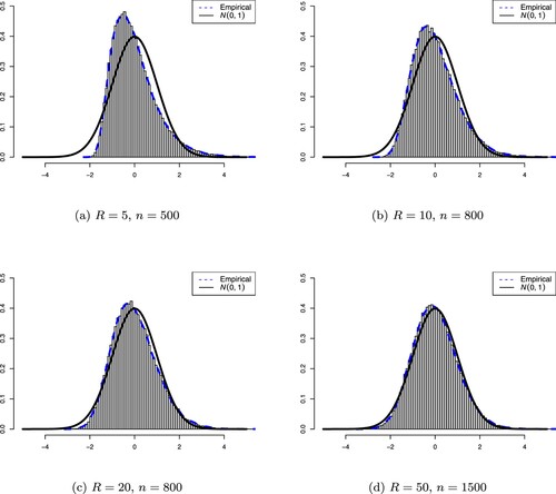
in Figure . In scenario (a) when R = 5 is too small, the empirical density curve of the standardized IPC test statistic deviates to some extent from the normal density function, even though the sample size n = 500 is large. Also, when R = 5, the empirical density is positively skewed, with more values clustered around the left tail while the right tail is slightly longer. The empirical density curve, however, is very well matched to the standard normal density curve when R increases, such as in scenario (c) when R = 20. This further emphasizes that R should be large enough (say, larger than 10) to ensure the normal approximation in Theorem 3.1 to hold.
Figure 1. Comparing the empirical distribution of the standardized IPC test statistic with the standard normal distribution. The blue broken line represents the empirical density and the black solid line represents the standard normal density. The empirical density is a kernel density estimate using Gaussian kernels based on 100000 values of . In each panel, the histogram of the standardized IPC test statistic is also displayed. (a) R = 5, n = 500. (b) R = 10, n = 800. (c) R = 20, n = 800 and (d) R = 50, n = 1500.
The following theorem allows us to bound the deviation of the IPC statistic when R is diverging, which is parallel to Theorem 3.1 in Ma et al. (Citation2022).
Theorem 3.2
Suppose for some
and there exists a positive constant
such that
for
,
. Then for any
,
(10)
(10) where
is a positive constant and
depends only on
.
Remark 3.1
He et al. (Citation2019) has also established a concentration inequality for the IPC statistic. However, their theoretical guarantee relies on a fixed number of categories (i.e., ). Thus, Theorem 3.2 is different to Lemma 4 in He et al. (Citation2019).
The condition for
, which is also used in Cui et al. (Citation2015) and Cui and Zhong (Citation2019), requires that the proportion of each category of
can not be too small. Indeed, the condition can be relaxed in a way that
is allowed to tend to 0 at a slow rate. Specifically, if we assume
for some
, then the probability in (Equation10
(10)
(10) ) will still converge to zero, but the convergence rate will be relatively slower. Note that Theorem 2.4 is a special case of Theorem 3.2 when
, i.e.,
is fixed, and the condition on
is automatically satisfied.
3.2. Extension of the IPC test
A natural application of Theorem 3.1 is to extend the IPC test to test independence between two continuous variables via the slicing technique. Consider two continuous random variables X and Z. Without loss of generality, we assume that the supports of X and Z are . We define a partition of the support of Z with a given positive integer R:
(11)
(11) where
,
. Each interval
is called a slice in the literature (Mai & Zou, Citation2015b; Yan et al., Citation2018). And a new random variable can be accordingly defined as
if and only if
for
. The IPC test can be applied to test independence between X and
. If the distribution of Z is known, we suggest a uniform slicing to partition Z such that
for
, where
is the cumulative distribution function of Z. However, in practice,
is usually unknown. But given observations
with sample size n, we can use
to estimate
for
, where
is the empirical distribution of Z. And
is regarded as an intuitive uniform slicing scheme (Yan et al., Citation2018). We also define
if and only if
for
,
. Now, we compute
as
where
, and
is the empirical conditional distribution of X based on the subjects for which
. We reject hypothesis
, if
for some given significance value
, where
is the standard normal distribution function.
Obviously, it is important to choose an appropriate R for testing independence. If R is too large, then the sample size in each slice is too small, making the estimate of the IPC index inaccurate. And if R is too small, then much information of Z may be lost, making the test power poor. In the slicing literature (Mai & Zou, Citation2015b; Yan et al., Citation2018; Zhong et al., Citation2021), a common choice is to set , where
is the integer part of x. And according to Theorem 3.1, we can also choose
. In practice, we recommend choosing
for some
, so that the sample size in each slice is about 20 to 50.
3.3. Comparison with the MV test
In this subsection, we would like to discuss the advantages of the IPC test compared to the MV test. As explained in Cui and Zhong (Citation2019), the MV index can be considered as the weighted average of Cramr-von Mises distances between
, the conditional distribution of X given Y = r, and
, the unconditional distribution function of X. Note that the IPC index can be viewed as a modification of the MV index by adding a weight function
. Such weight function is large for
near 0 and 1, and smaller near
. Hence, the IPC test emphasizes more on the difference between
and
near the tail of
. As it is known,
. Accordingly, the IPC test is more sensitive to tail differences among the conditional distributions. In the following, we consider the test of independence between a continuous random variable and a categorical variable with a relatively large number of classes (i.e., R is large) and the test of independence for two continuous random variables, and further illustrate the IPC test's sensitivity to differences in the tails of the conditional distributions through numerical simulations.
1. When R is large or is allowed to diverge. In this case, we recommend using a normal distribution to approximate the IPC test's null distribution due to Theorem 3.1. It is not surprising that given a large R, IPC test still retains sensitivity to tail differences when using a normal distribution instead of to calculate p-value. The following example is used to illustrate this issue.
Let with
, for
. When Y = r, generate
, where
, W and
are independent,
and
. To intuitively gain some understanding of our simulation setting, set p = 0.8. We draw the conditional distributions of X given Y = 1 and Y = 5, respectively in Figure . It is easy to see that the conditional distributions differ from each other only at their right tails. We choose the sample size n = 400, and p = 0.7, 0.75, 0.8, 0.85, 0.9. We apply the IPC test and the MV test, and compute the p-values for these two tests by using their approximated normal distributions. The empirical powers of these two tests based on 500 replicates at the significance level
are presented in Table . To further validate the robustness of the IPC test against heavy-tails, we further consider
in the above setting. The empirical powers are also shown in Table . A larger p indicates that the differences among the conditional distributions occur in a more extreme right tail end, and thus are more difficult to detect the dependence between X and Y. We can see from Table that the IPC test is significantly more powerful than the MV test when p<0.9. When p = 0.9, neither the IPC nor the MV has sufficient statistical power to detect the dependence between X and Y. The simulation validates that the IPC test has a better power to tail differences among the conditional distributions. In Example 4.1 we will compare with other existing methods to further validate the IPC test's sensitivity towards tail differences.
Figure 2. Panel (a) shows the pair of conditional distributions. The blue solid line represents the conditional distribution of X given Y = 1, that is, where
; and the red dot-dash line represents the conditional distribution of X given Y = 5, that is,
where
. Panel (b) shows the corresponding conditional density functions.
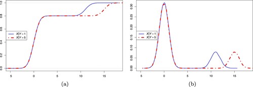
Table 3. Test of independence between a continuous variable and a categorical variable with R = 20 classes.
2. Testing independence between continuous random variables. We follow the notation in Section 3.2. Let X and Z be two continuous random variables. It is natural to expect that the IPC test will be more powerful than the MV test to detect the tail differences among the conditional distribution of X given Z. Consider a straightforward extension of the IPC index in (Equation5(5)
(5) ) and define the following index between X and Z:
(12)
(12) where
is the conditional distribution of X given Z = z, and
and
are the distributions of X and Z, respectively. Given a positive integer R and a corresponding uniform slicing scheme
defined as in (Equation11
(11)
(11) ) with
for
, recall that
if and only if
. Under certain mild conditions, Ma et al. (Citation2022) has shown that
, as
.
From (Equation12(12)
(12) ), again, we have some insights that the IPC test of independence emphasizes more on the difference between
and
near the tail of
. We use a toy sample to further illustrate this issue. Generate
, and generate
, where
. We still consider two settings of W: (i)
and (ii)
. Choose the sample size n = 400, and p = 0.7, 0.75, 0.8, 0.85, 0.9. We follow the step in Section 3.2 and choose R = 20 to conduct the test of independence. Table presents the empirical powers of IPC and MV tests based on 500 replicates at the significance level
. IPC test outperforms the MV test in these settings. Note that when p = 0.8, the MV test is almost invalid. However, the IPC test still has a reasonably acceptable power.
Table 4. Test of independence between two continuous random variables.
4. Numerical studies and data application
4.1. Numerical studies
In this section, we assess the finite-sample performance of the IPC test by comparing with some powerful methods proposed in recent years: the MV test (Cui & Zhong, Citation2019), the distance correlation (DC) test (Székely et al., Citation2007), the HHG test (Heller et al., Citation2012, Citation2016) and the Hilbert-Schmidt independence criterion (HSIC) test (Gretton et al., Citation2005, Citation2007; Pfister et al., Citation2018). The R packages energy, HHG, and dHSIC are used to implement the DC test, the HHG test and the HSIC test, respectively. Note that the DC test can not be directly applied to a categorical variable, so in our simulations we will transfer a categorical variable with R categories into a random vector with R−1 binary dummy variables and apply dcov.test to this dummy vector instead of the original data. For the DC, HHG, and HSIC tests, the permutation test with K = 200 is used to calculate the p-value.
Example 4.1
In this example, we evaluate the performance of IPC test for the large-R case. Let R = 15, and we consider the following two cases.
Model 1.1. Generate with equal probabilities. And let
, where
for
, and
for l = 4, 5, j = 0, 1, 2. For Y = r, generate
, where
,
,
.
Model 1.2. Generate . And let
, where
. B, U are the same as in Model 1.1.
Let n = 400. In Model 1.2, we uniformly slice Y into a categorical variable with R = 15 classes in order to apply the IPC and MV tests. Let p vary from 0 to 1 in both two models. We compute the p-value for the IPC test by using the asymptotic distribution in Theorem 3.1. The empirical power of each test based on 500 simulations at the significance level is shown in Figure . Note that, when p = 1, X is independent with Y in both models. We deliberately report the results, i.e., the type I error rates of each test, in Table . The type I error rates of the IPC test (and other tests) are close to the nominal significance level
, which further supports Theorem 3.1. Figure clearly shows that the IPC test outperforms other competitors. And the power differences between IPC test and MV test exceed 0.25 when p = 0.6 for both models.
Figure 3. Comparison of powers of several tests of independence against different p in Example 4.1. In each case, 500 simulations are used to estimate the power. (a) Model 1.1 and (b) Model 1.2.
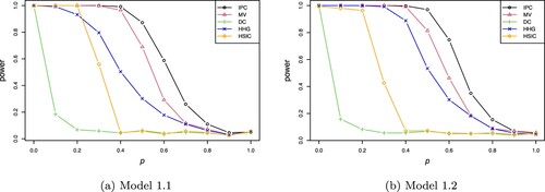
Table 5. Empirical type I error rates at the significance level in Example 4.1.
Looking further into the models considered in this example. In both Model 1.1 and Model 1.2, the conditional distributions of X given Y differ from each other only in their right tails when p>0.5. A larger p indicates that the conditional distribution functions differ from each other in a more extreme tail end. And when p = 1, X and Y are independent. Thus it could be more difficult to detect the dependence between X and Y for a larger p<1. As a result, we can see from Figure that the power of each test decreases with the growth of p. Among the tests considered, the DC test and the HSIC test perform the worst in both models. Their powers rapidly decrease to near 0 when p increases to 0.4. It can be seen that the IPC test and the MV test have a better performance compared to other tests. Furthermore, the IPC test has a significant higher power than the MV test when p is between 0.6 and 0.8 in both models. This further supports our observation in Section 3.3 that the IPC test is more sensitive to tail differences.
Example 4.2
This example considers a Poisson regression model. Let , where
,
,
. Let Y = Z if
; otherwise Y = 9. As a consequence, Y is a 10-categories variable. Consider
. We apply the testing methods to test independence between Y and
, Y and
, respectively. And the asymptotic normal distribution in Theorem 3.1 is used to compute p-value for the IPC test. The empirical powers of each test based on 500 replications are summarized in Table . The IPC test has most excellent power performances in all settings. The HHG test and the HSIC test perform poorly when the sample size
.
Table 6. Empirical powers of each test at the significance level against the sample sizes in Example 4.2.
The power of the IPC test is only slightly higher than that of the MV test. However, it is significantly higher than that of HHG and HSIC. The DC test has moderate performance, inferior to the MV test, but better than HSIC.
Example 4.3
In this example, we evaluate the power of the IPC test in testing independence between continuous variables. Simulations are carried out with sample size n = 400. We choose R = 15 to implement the IPC test. Generating , the following alternatives are considered.
Linear:
, where γ is a noise parameter ranging from 0 to 1, and
Quadratic:
Step function:
W-shaped:
Sinusoid:
Ellipse:
To conduct the IPC test and the MV test, we uniformly slice Z into a categorical variable Y with R = 15 classes. The choices of the coefficients in all of the above are to make sure that a full range of powers can be observed when γ varies from 0 to 1. In addition to the test methods mentioned before, in this example, we further consider a comparison with a new test, the modified Blum-Kiefer-Rosenblatt (MBKR) test (Zhou & Zhu, Citation2018) which is applied for testing independence between continuous variables. Figure presents the empirical power of each test based on 500 simulations at the significance level . We see from the figure that the IPC test performs quite excellent when the relationship has an oscillatory nature (the W-shaped and the sinusoid). It is also better than other competitors for the step function, and comparably well to the MBKR test for the quadratic function. However, the IPC test has poor performance compared to other tests for some smooth alternatives: the linear and the ellipse. For the linear function, the MBKR test has the highest performance. IPC test has comparable performance to HSIC. For the ellipse function, HHG test has the highest power and DC test performs the poorest. The performance of the IPC test, on the other hand, is moderate.
Figure 4. Comparison of powers of several tests of independence in Example 4.3. The noise level increases from left to right. In each case, 500 simulations are used to estimate the power of each test. (a) Linear. (b) Quadratic. (c) Step function. (d) W-shaped. (e) Sinusoid and (f) Ellipse.
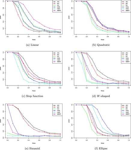
We give an intuitive explanation here for the excellent performance of the IPC test in detecting oscillatory relationships. Denote as the random variable which follows the conditional distribution of X given Y = r. By simple calculation, we find that if X and Z have an oscillatory relationship, then the variances of
differ from each other more significantly. As a comparison, if X and Z have a linear relationship, then
. Consequently, the IPC test has a higher test power when there is an oscillatory relationship between X and Z.
4.2. Real data application
Example 4.4
We consider a data set from AIDS Clinical Trials Group Protocol 175 (ACTG175), which is available from the R package speff2trial. Many researchers have studied this data set, such as Tsiatis et al. (Citation2008), Zhang et al. (Citation2008), Lu et al. (Citation2013) and Zhou et al. (Citation2020). The data set contains 2139 HIV-infected subjects. And all the subjects were randomized to four different treatment groups with equal probability: zidovudine (ZDV) monotherapy, ZDV+didanosine (ddI), ZDV+zalcitabine, and ddI monotherapy. In addition to the treatment indicators indicating which group each subject was assigned to, the data contains many other important variables, such as the CD4 count at weeks post-baseline (CD420), the CD4 count at baseline (CD40), the history of intravenous drug use, et al.
In this study, in order to get more elaborated results, we only consider the subjects under ZDV+zalcitabine groups (524 subjects) in the following analysis. The goal of our study is to check whether the treatment effect under ZDV + zalcitabine groups is dependent on some other covariates. Following Hammer et al. (Citation1996) and Tsiatis et al. (Citation2008), we use the change from baseline to weeks in CD4 cell count, i.e., CD420−CD40, to measure the treatment effect. And the covariates of interest are listed below: history of intravenous drug use (
no,
yes), gender (
female,
male), antiretroviral history (
naive,
experienced), age, and CD8 count at baseline (CD80). Thus the first three covariates are categorical, and the last two are continuous covariates. Let
, and then there are 5 candidates Y. The null hypotheses are listed as follows.
We apply the IPC, MV, DC, HHG and HSIC tests to these five hypotheses. The permutation test with K = 1000 permutated times is used for DC, HHG and HSIC tests to compute the p-values. And for and
, we follow the approach in Section 3.2 to slice Y into a categorical variable with 15 classes to implement the IPC test and MV test. Table summarizes the p-values of each test. If we only consider the significance level
, then we observe that all the tests reject
,
and
, and accept
. That is, the treatment effect under the ZDV+zalcitabine group depends on antiretroviral history, age and CD80, but not on gender. Regarding the history of intravenous drug use, the IPC, DC, HHG and HSIC tests declare statistical dependence between this and the treatment effect. However, the MV test has a p-value larger than 0.05, and thus it can not reject
. We draw the empirical conditional distributions of X given Y = 0 and 1 as well as the side-by-side boxplots in Figure , where
. We see that the conditional distributions of X are different across different Y. However, the difference is relatively small and mainly occurs in the right tails. According to the discussion in Section 3.3, IPC test will be more powerful in such case. Also, the categories of Y are very unbalanced with
and
, making the MV test more difficult to detect the dependence between X and Y.
Figure 5. The left panel shows the empirical conditional distributions of given Y = 0 and Y = 1. And the right panel shows the side-by-side boxplots of
against Y = 0 and Y = 1. Here
history of intravenous drug use.
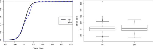
Table 7. The p-values of each test in Example 4.4.
5. Discussion
In this paper, we studied the IPC test of independence between a continuous variable X and a categorical variable Y. When the number of categories of Y is fixed, the IPC test statistic is in essence the k-sample Anderson Darling test statistic, and its theoretical properties were studied in Scholz and Stephens (Citation1987). Our work mainly focused on two aspects. First, we derived the convergence rate of the IPC statistic to the IPC index and thus a lower bound of the power of the test at a given significance level with a finite sample size could be derived. Second, we showed that the standardized test statistic has an asymptotic normal distribution when the number of categories R diverges to infinity with the sample size. A distinguished merit is thereby shared by the IPC test, that is, its critical values can be easily obtained by using an approximated normal distribution when R is relatively large. As an application, we extended the IPC test to test independence between two continuous random variables. We uniformly slice a continuous variable into a discrete variable in order to apply the IPC test. And by allowing more slices as the sample size increases, the IPC test is allowed to gain more test power. The proposed test was compared to the DC test, HHG test, HSIC test and MV test on many simulation experiments. The results showed that the IPC test has a better performance in many scenarios. It is also possible to consider more different slicing schemes for independence testing of continuous variables. We left it for further research.
Disclosure statement
No potential conflict of interest was reported by the author(s).
Additional information
Funding
References
- Csörgö, S. (1985). Testing for independence by the empirical characteristic function. Journal of Multivariate Analysis, 16(3), 290–299. https://doi.org/10.1016/0047-259X(85)90022-3
- Cui, H., Li, R., & Zhong, W. (2015). Model-free feature screening for ultrahigh dimensional discriminant analysis. Journal of the American Statistical Association, 110(510), 630–641. https://doi.org/10.1080/01621459.2014.920256
- Cui, H., & Zhong, W. (2018). A distribution-free test of independence and its application to variable selection. Available at arXiv:1801.10559.
- Cui, H., & Zhong, W. (2019). A distribution-free test of independence based on mean variance index. Computational Statistics & Data Analysis, 139, 117–133. https://doi.org/10.1016/j.csda.2019.05.004
- Dvoretzky, A., Kiefer, J., & Wolfowitz, J. (1956). Asymptotic minimax character of the sample distribution function and of the classical multinomial estimator. The Annals of Mathematical Statistics, 27(3), 642–669. https://doi.org/10.1214/aoms/1177728174
- Gretton, A., Bousquet, O., Smola, A., & Schölkopf, B. (2005). Measuring statistical dependence with hilbert-schmidt norms. In S. Jain, H. U. Simon, & E. Tomita (Eds.), Algorithmic learning theory (pp. 63–77). Springer Berlin Heidelberg.
- Gretton, A., Fukumizu, K., Teo, C. H., Song, L., Schölkopf, B., & Smola, A. J. (2007). A kernel statistical test of independence. In Proceedings of the 20th International Conference on Neural Information Processing Systems (pp 585–592). Curran Associates Inc. NIPS'07.
- Hall, P., & Heyde, C. C (1980). Martingale limit theory and its application, Probability and mathematical statistics, Inc, Academic Press [Harcourt Brace Jovanovich, Publishers].
- Hammer, S. M., Katzenstein, D. A., Hughes, M. D., Gundacker, H., Schooley, R. T., Haubrich, R. H., Henry, W. K., Lederman, M. M., Phair, J. P., Niu, M., Hirsch, M. S., & Merigan, T. C. (1996). A trial comparing nucleoside monotherapy with combination therapy in hiv-infected adults with cd4 cell counts from 200 to 500 per cubic millimeter. New England Journal of Medicine, 335(15), 1081–1090. https://doi.org/10.1056/NEJM199610103351501
- He, S., Ma, S., & Xu, W. (2019). A modified mean-variance feature-screening procedure for ultrahigh-dimensional discriminant analysis. Computational Statistics & Data Analysis, 137, 155–169. https://doi.org/10.1016/j.csda.2019.02.003
- Heller, R., Heller, Y., & Gorfine, M. (2012). A consistent multivariate test of association based on ranks of distances. Biometrika, 100(2), 503–510. https://doi.org/10.1093/biomet/ass070
- Heller, R., Heller, Y., Kaufman, S., Brill, B., & Gorfine, M. (2016). Consistent distribution-free k-sample and independence tests for univariate random variables. Journal of Machine Learning Research, 17(29), 1–54.
- Hoeffding, W. (1948). A non-parametric test of independence. The Annals of Mathematical Statistics, 19(4), 546–557. https://doi.org/10.1214/aoms/1177730150
- Jiang, B., Ye, C., & Liu, J. S. (2015). Nonparametric k-sample tests via dynamic slicing. Journal of the American Statistical Association, 110(510), 642–653. https://doi.org/10.1080/01621459.2014.920257
- Lu, W., Zhang, H. H., & Zeng, D. (2013). Variable selection for optimal treatment decision. Statistical Methods in Medical Research, 22(5), 493–504. https://doi.org/10.1177/0962280211428383
- Ma, W., Xiao, J., Yang, Y., & Ye, F. (2022). Model-free feature screening for ultrahigh dimensional data via a Pearson chi-square based index. Journal of Statistical Computation and Simulation, 92(15), 3222–3248. https://doi.org/10.1080/00949655.2022.2062358
- Mai, Q., & Zou, H. (2015a). Sparse semiparametric discriminant analysis. Journal of Multivariate Analysis, 135, 175–188. https://doi.org/10.1016/j.jmva.2014.12.009
- Mai, Q., & Zou, H. (2015b). The fused Kolmogorov filter: A nonparametric model-free screening method. The Annals of Statistics, 43(4), 1471–1497. https://doi.org/10.1214/14-AOS1303
- Ni, L., & Fang, F. (2016). Entropy-based model-free feature screening for ultrahigh-dimensional multiclass classification. Journal of Nonparametric Statistics, 28(3), 515–530. https://doi.org/10.1080/10485252.2016.1167206
- Ni, L., Fang, F., & Shao, J. (2020). Feature screening for ultrahigh dimensional categorical data with covariates missing at random. Computational Statistics & Data Analysis, 142, Article 106824. https://doi.org/10.1016/j.csda.2019.106824
- Ni, L., Fang, F., & Wan, F. (2017). Adjusted Pearson chi-square feature screening for multi-classification with ultrahigh dimensional data. Metrika, 80(6–8), 805–828. https://doi.org/10.1007/s00184-017-0629-9
- Pfister, N., Bühlmann, P., Schölkopf, B., & Peters, J. (2018). Kernel-based tests for joint independence. Journal of the Royal Statistical Society. Series B. Statistical Methodology, 80(1), 5–31. https://doi.org/10.1111/rssb.12235
- Rosenblatt, M. (1975). A quadratic measure of deviation of two-dimensional density estimates and a test of independence. The Annals of Statistics, 3(1), 1–14. https://doi.org/10.1214/aos/1176342996
- Scholz, F.-W., & Stephens, M. A. (1987). k-sample Anderson–Darling tests. Journal of the American Statistical Association, 82(399), 918–924. https://doi.org/10.2307/2288805
- Székely, G. J., & Rizzo, M. L. (2009). Brownian distance covariance. The Annals of Applied Statistics, 3(4), 1236–1265. https://doi.org/10.1214/09-AOAS312
- Székely, G. J., Rizzo, M. L., & Bakirov, N. K. (2007). Measuring and testing dependence by correlation of distances. The Annals of Statistics, 35(6), 2769–2794. https://doi.org/10.1214/009053607000000505
- Tsiatis, A. A., Davidian, M., Zhang, M., & Lu, X. (2008). Covariate adjustment for two-sample treatment comparisons in randomized clinical trials: A principled yet flexible approach. Statistics in Medicine, 27(23), 4658–4677. https://doi.org/10.1002/sim.3113
- Xu, K., Shen, Z., Huang, X., & Cheng, Q. (2020). Projection correlation between scalar and vector variables and its use in feature screening with multi-response data. Journal of Statistical Computation and Simulation, 90(11), 1923–1942. https://doi.org/10.1080/00949655.2020.1753057
- Yan, X., Tang, N., Xie, J., Ding, X., & Wang, Z. (2018). Fused mean-variance filter for feature screening. Computational Statistics & Data Analysis, 122, 18–32. https://doi.org/10.1016/j.csda.2017.10.008
- Zhang, M., Tsiatis, A. A., & Davidian, M. (2008). Improving efficiency of inferences in randomized clinical trials using auxiliary covariates. Biometrics, 64(3), 707–715. https://doi.org/10.1111/j.1541-0420.2007.00976.x
- Zhang, Y., Chen, C., & Zhu, L. (2022). Sliced independence test. Statistica Sinica, 32(Special onlline issue), 2477–2496. https://doi.org/10.5705/ss.202021.0203
- Zhong, W., Wang, J., & Chen, X. (2021). Censored mean variance sure independence screening for ultrahigh dimensional survival data. Computational Statistics & Data Analysis, 159, Article 107206. https://doi.org/10.1016/j.csda.2021.107206
- Zhou, N., Guo, X., & Zhu, L. (2020). A projection-based model checking for heterogeneous treatment effect. Available at arXiv:2009.10900.
- Zhou, Y., & Zhu, L. (2018). Model-free feature screening for ultrahigh dimensional datathrough a modified Blum-Kiefer-Rosenblatt correlation. Statistica Sinica, 28(3), 1351–1370. https://doi.org/10.5705/ss.202016.0264
- Zhu, L., Xu, K., Li, R., & Zhong, W. (2017). Projection correlation between two random vectors. Biometrika, 104(4), 829–843. https://doi.org/10.1093/biomet/asx043
Appendix
Proof of theorems
This appendix contains the technical proofs of Lemma 2.2 and Theorem 3.1. Lemma 2.1 and Theorem 2.4 are direct corollaries of Theorem 3.2, and the proof of Theorem 3.2 follows from Lemma 4 in Ma et al. (Citation2022), and thus their proofs are omitted.
A.1. Notations and preliminaries
Recall that the IPC index of , where X is a continuous random variable with support
and
is a categorical variable with R categories is defined as
where
is the distribution function of X,
,
,
and
,
. And given i.i.d. samples
for
, the IPC statistic is defined as
where
,
,
,
, and
for
.
We first provide a proof of Lemma 2.2.
Proof of Lemma 2.2.
It is obvious that if and only if X and Y are independent. By noticing that
and
, we have
Hence we have
.
Next, we give some preparations for the proof of Theorem 3.1. For given constant C>0, let ,
,
and
. Then we have the following lemmas.
Lemma A.1
Let and
. Then
Proof.
It is easy to show that
Hence by Dvoretzky–Kiefer–Wolfowitz (DKW) inequality (Dvoretzky et al., Citation1956),
Similarly, we have
.
Lemma A.2
.
Proof.
Note that
Then,
A.2. Proof of Theorem 3.1
To avoid any ambiguity, Theorem 3.1 considers a sequence of problems indexed by ,
where the sample size
, the number of categories
, and let
denote the categorical variable with
categories and
,
. From now on, we shall omit the subscript unless specifically mentioned. Moreover, in Section A.2, we should keep in mind that X and Y are independent.
A.2.1. Architecture of the proof
Our aim here is to provide a general overview of the proof of Theorem 3.1. At a high level, the general structure is fairly simple. And to make the structure clear, we divide the proof into three parts.
First, given a positive constant C, we substitute
Fixing C = 6, let
Finally, consider
Combined with Lemmas A.1 and A.2, the proof in part 1 is not difficult. And the proofs in part 2 and part 3 follow from Cui and Zhong (Citation2018) and Cui and Zhong (Citation2019) with a small modification.
A.2.2. Part 1
We summarize the conclusion we want to prove in part 1 into the following lemma.
Lemma A.3
For a fixed constant C, let
For simplicity, write
, and
. Then if
, and under condition that X and Y are independent, we have
Proof.
Let
Then
Since
we have
So,
. Then
Since
, we have
Hence,
. Next, let
Let
be the ordered statistics of
. Since X is continuous, there are no ties among
. We can assume that
. Let
, and define
Indeed, we have
. And
Similarly, we also have
. Therefore,
Finally, according to Lemma A.2,
Hence
A.2.3. Part 2
Recall that
and
The following lemma is what we want to prove in part 2.
Lemma A.4
If , and Under
: X and Y are independent, then
Proof.
For simplicity, write . Given C = 6, according to Lemma A.3, and under the condition that
, we have
(A1)
(A1) Let
Next, we follow the proof of Lemma A.1 in Cui and Zhong (Citation2019), and show that
Let
. By the DKW inequality, we have
Here, the second equality follows by
and the last equality follows by
Indeed,
and
where the first inequality follows by the DKW inequality. Hence,
and similarly
. Therefore, we have
(A2)
(A2) Combining (EquationA1
(A1)
(A1) ) and (EquationA2
(A2)
(A2) ), we have
To complete the proof, we only need to show that
It is enough to show that
Without loss of generality, let
be the uniform distribution function, since we can make the transformation
for the continuous random variable X. And
For any
, it can be easily proved that
where
and
. Then
where
. And be careful here that
is different from
defined above.
Since under
, we have
under
if one of
is different from the other three. Then we have
And also, we have
and
Hence,
So,
A.2.4. Part 3
Now, we will complete the proof of Theorem 3.1.
Proof of Theorem 3.1.
Let . Without loss of generality, we assume that
. Then
for
. According to Lemma A.4, we have
Then under the condition
, we have
, and thus
, i.e.,
Hence, we only need to prove that
as
.
Recall that , where
and
. We first give some important facts:
for all ,
, where C is a constant and
if r = s and
, otherwise.
We prove (ii). Without loss of generality, we assume that .
And
The last inequality is because, if
, then
; if
, then
; if
, then
.
(iii) . This result can be found in Cui and Zhong (Citation2018) and Cui and Zhong (Citation2019).
Write
where
and
Note that,
and
Hence,
where C is a constant. Next, we only need to show that
Note that
, and
The last equality holds because
Let
be the σ-field generated by a set of random variables
,
. We see that
is the summation of a martingale difference sequence with
and
. According to Hall and Heyde (Citation1980), we need to prove
.
Thus we have
where
and
Since
, and
where C and
are constants. Thus
. And
, and
Thus,
. On the other hand
where C,
and
are constants. By the central limit theorem of the martingale difference (Hall & Heyde, Citation1980), we have
as
. This completes the proof.