
 ?Mathematical formulae have been encoded as MathML and are displayed in this HTML version using MathJax in order to improve their display. Uncheck the box to turn MathJax off. This feature requires Javascript. Click on a formula to zoom.
Abstract
Missing data are unavoidable in longitudinal clinical trials, and outcomes are not always normally distributed. In the presence of outliers or heavy-tailed distributions, the conventional multiple imputation with the mixed model with repeated measures analysis of the average treatment effect (ATE) based on the multivariate normal assumption may produce bias and power loss. Control-based imputation (CBI) is an approach for evaluating the treatment effect under the assumption that participants in both the test and control groups with missing outcome data have a similar outcome profile as those with an identical history in the control group. We develop a robust framework to handle non-normal outcomes under CBI without imposing any parametric modeling assumptions. Under the proposed framework, sequential weighted robust regressions are applied to protect the constructed imputation model against non-normality in the covariates and the response variables. Accompanied by the subsequent mean imputation and robust model analysis, the resulting ATE estimator has good theoretical properties in terms of consistency and asymptotic normality. Moreover, our proposed method guarantees the analysis model robustness of the ATE estimation in the sense that its asymptotic results remain intact even when the analysis model is misspecified. The superiority of the proposed robust method is demonstrated by comprehensive simulation studies and an AIDS clinical trial data application.
1. Introduction
1.1. Missing data in clinical trials
Analysis of longitudinal clinical trials often presents difficulties as, inevitably, some participants do not complete the study, thereby creating missing outcome data. Additionally, outcomes among participants who complete the study may not be of interest on account of intercurrent events such as the initiation of rescue therapy before the analysis time point. With the primary interest focusing on evaluating the treatment effect, the approach to handling missingness plays an essential role and has gained substantial attention from the US Food and Drug Administration (FDA) and National Research Council (R. J. Little et al., Citation2012). The ICH E9(R1) addendum provides a detailed framework for defining estimands to target the major clinical question in a population-level summary considering intercurrent events that may cause additional missingness (ICH, Citation2021).
The missing at random (MAR; Rubin, Citation1976) mechanism is often invoked in analyses that seek to evaluate treatment efficacy. However, MAR is unverifiable and may not be practical in some clinical trials. Further, if the response at the primary time point is of interest regardless of whether participants have complied with the test or comparator treatments through the primary time point (corresponding to a ‘treatment policy’ intercurrent event strategy), an analysis based on the MAR assumption would not be appropriate, because such an analysis would assume that responses in those who dropped out followed the same trajectory as in those who remained on treatment. A more plausible assumption would be that any treatment effect obtained while a participant was in the study was lost after discontinuation from the study, leading to a missing not at random (MNAR) assumption that responses in participants who failed to complete treatments in both groups behaved similarly to the observed responses in the control group. Drawn on the idea of the zero-dose model in R. Little and Yau (Citation1996), Carpenter et al. (Citation2013) referred to this scenario as control-based imputation (CBI). Since CBI represents a deviation from MAR, it is widely used in sensitivity analyses to explore the robustness of the study results against the untestable MAR assumption (e.g., Carpenter et al., Citation2013; Cro et al., Citation2016; Mack et al., Citation2019). Furthermore, an increasing number of clinical studies have applied this approach to primary analyses irrespective of the compliance status, such as clinical trials that target weight loss or chronic disease (e.g., O'Neil et al., Citation2018; Tan et al., Citation2021). Several specific CBI settings, which include jump-to-reference (J2R), copy reference (CR), copy increments in reference (CIR), and last mean carried forward (LMCF) and will be summarized in Section 3, are proposed by Carpenter et al. (Citation2013) to characterize different types of similarity between the missing outcomes in the treated group and the observed outcomes in the control group. Throughout the paper, we focus on J2R as one application of CBI that is frequently seen in the FDA statistical review and evaluation reports (e.g., US Food & Drug Administration, Citation2016) with the assumption that the missing outcomes in the treatment group will have the same outcome mean profile as those with identical historical information in the control group. Our goal is to assess the average treatment effect (ATE) under J2R. Extensions to other CBI scenarios follow the same idea.
1.2. Multiple imputation and the existing robust methods
Multiple imputation (MI; Rubin, Citation2004) followed by a mixed-model with repeated measures (MMRM) analysis is a common approach to analyzing longitudinal clinical trial data under CBI. The simple implementation and high flexibility of MI underlie the recommendation of this approach by the regulatory agencies (R. J. Little et al., Citation2012). In the implementation of MI, distributional assumptions such as normality are often assumed for simplicity and robustness against moderate model misspecification (Mehrotra et al., Citation2012). One common MI procedure in longitudinal clinical trials under J2R is summarized in the following steps.
| Step 1. | For the control group, fit a sequential regression for the observed data at each visit point against the available history to construct the imputation model under J2R. | ||||
| Step 2. | Impute the missing data sequentially to form multiple imputed datasets: for individuals who have missing values at each visit, impute the missing components from the estimated imputation model in Step 1 and create the imputed dataset. | ||||
| Step 3. | For each imputed dataset, perform the complete data analysis and assess the ATE. | ||||
| Step 4. | Combine the estimation results from those imputed datasets and obtain the MI estimator along with its variance estimator by Rubin's rule. | ||||
Traditionally, the imputation model in Step 1 and the analysis model in Step 3 are obtained from an MMRM analysis and rely heavily on the parametric modeling assumptions, where we assume an underlying normal distribution for both the observed and the imputed data. In reality, the distribution of the outcomes may contradict the normality assumption on account of the existence of extreme values. A motivating CD4 count dataset in Section 2 further addresses that a simple transformation such as the log transformation sometimes cannot fix the non-normality issue (Mehrotra et al., Citation2012). Applying the methods that rely on the normal distribution to the dataset may produce bias and power loss. To tackle this issue in longitudinal clinical trials under MAR, Mogg and Mehrotra (Citation2007) and Mehrotra et al. (Citation2012) modified the analysis model in Step 3 by substituting the conventional least squares (LS) regression in the full-data analysis step of MI with rank-based regression (Jaeckel, Citation1972) or Huber robust regression (Huber, Citation1973) to down-weight the impact of non-normal response values. However, the imputation model still depends on normality as required by MI in their modified robust approaches.
Moreover, the MI estimator is not efficient in general. The inefficiency becomes more serious when it comes to interval estimation. The variance estimation using Rubin's rule may be inconsistent even when the imputation and analysis models are the same correctly specified models (Robins & Wang, Citation2000). Under MNAR, overestimation raised by Rubin's variance estimator is more pronounced (e.g., Guan & Yang, Citation2019; G. F. Liu & Pang, Citation2016; S. Liu et al., Citation2022; Yang & Kim, Citation2016; Yang et al., Citation2021). One can instead use bootstrap to obtain a consistent variance estimator, but this exaggerates the computational cost. These unsatisfactory performances of MI motivate us to develop a robust approach to accommodate outliers or heavy-tailed errors and obtain a valid variance estimator without the reliance on parametric models under non-normality and MNAR.
1.3. Our contribution: a robust framework
We develop a robust framework to evaluate the ATE for non-normal longitudinal outcomes with missingness under CBI, where the robust regression in conjunction with mean imputation is applied to relax the parametric modeling assumption required by MI in both the imputation and analysis stages. Inspired by the sequential linear regression model in many longitudinal studies, where the current outcomes are regressed recursively on the historical information (Tang, Citation2017), we replace the LS estimator with the estimator obtained by minimizing the robust loss function such as the Huber loss, the absolute loss (Huber, Citation2004), and the ε-insensitive loss (Smola & Schölkopf, Citation2004), to mitigate the impact of non-normality in the response variable. While robust regression lacks the protection against outliers in the covariates (Chang et al., Citation2018), a weighted sequential robust regression model is put forward using the idea in Carroll and Pederson (Citation1993) to down-weight the influential covariates by a robust Mahalanobis distance. Followed by mean imputation and a robust analysis step, the estimator from our proposed method has solid theoretical guarantees in terms of consistency and asymptotic normality.
Rosenblum and Van Der Laan (Citation2009) establish a robustness result of the hypothesis test for randomized clinical trials with complete data; i.e., for a wide range of analysis models, testing the existence of the non-zero ATE has an asymptotically correct type-1 error even under model misspecification. However, they focus only on LS estimators when no ATE exists; and the properties of robustness remain unclear when the parameters are estimated via the robust loss function under any arbitrary ATE value. To avoid this ambiguity, we extend the robustness properties to our proposed method for ATE estimation in the context of missing data. We formally show that the ATE estimator obtained from the non-LS loss functions, including the Huber loss, the absolute loss, and the ϵ-insensitive loss, is analysis model-robust in the sense that its asymptotic properties remain the same even when the analysis model is incorrectly specified.
The rest of the paper is organized as follows. Section 2 uses a real-data example to motivate the need for a robust method. Section 3 introduces the setup and presents an overview of the existing methods. Section 4 describes the proposed robust method. Section 5 provides the asymptotic results of the ATE estimator. Section 6 conducts comprehensive simulation studies to validate the proposed method. Section 7 returns to the motivating example to illustrate the performance of the robust method in practice. Concluding thoughts are provided in Section 8.
2. A motivating application
Study 193A conducted by the AIDS Clinical Trial Group compared the effects of dual or triple combinations of the HIV-1 reverse transcriptase inhibitors (Henry et al., Citation1998). The data consist of the longitudinal CD4 counts collected at baseline and during the first 40 weeks of follow-up, with the fully-observed baseline covariates as age and gender. Participants were randomly assigned among four treatments regarding dual or triple therapies. We focused on the treatment comparison between arm 1 (zidovudine alternating monthly with 400 mg didanosine) and arm 2 (zidovudine plus 400 mg of didanosine plus 400 mg of nevirapine). As arm 1 involves fewer combinations of inhibitors, we viewed it as the control group. We then deleted the individuals in these arms with missing baseline CD4 counts, partitioned the time into discrete intervals ,
,
,
and
, and created a dataset with a monotone missingness pattern. The detailed data manipulation procedure is given in Section S4 in the supplementary material.
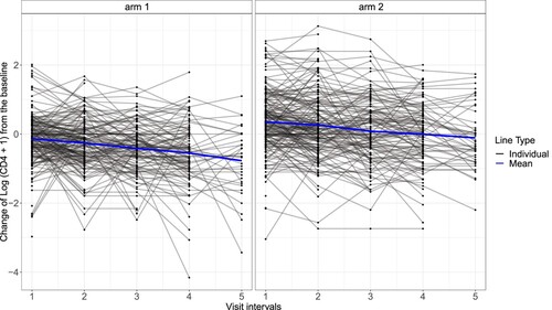
Since the original CD4 counts were highly skewed, we performed a log transformation to get the transformed CD4 counts as and used them as the outcomes of interest. Figure presents spaghetti plots of the transformed CD4 counts change from the baseline. Although there were no notable outliers, severe missingness was evident, with only 34 of 320 participants in arm 1 and 46 of 330 participants in arm 2 completing the trial. The high dropout rates reflected a typical missing data issue in longitudinal clinical trials, leading to the need to impute the missing values to prevent substantial information loss and potential bias from focusing on only the complete data.
Figure 1. Spaghetti plots of the change of the log-transformed CD4 count data from the baseline separated by the two treatments. The blue line represents the mean of the observed outcomes at each visit point. The black lines refer to the individual outcome profiles.
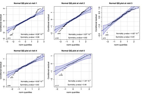
We checked the normality of the transformed data by fitting sequential linear regressions on the current outcomes against all historical information and examining the conditional residuals at each visit point for model diagnosis. Figure presents the results from the Shapiro-Wilk test and normal QQ plots. Each normality test indicates a violation of the normal assumption, and the normal QQ plots reveal that the CD4 counts remained heavy-tailed even after the log transformation. Under this circumstance, potentially biased and inefficient treatment effect estimates may occur when applying the conventional MI method along with the MMRM analysis. It motivates the development of a robust method to assess the treatment effect under non-normality.
Figure 2. Normal QQ plots of the conditional residuals at each visit. The conditional residuals were obtained by fitting the sequential linear regressions on the current outcomes against the available history and calculating the residuals at each visit. The p-values for the Shapiro-Wilk test and the symmetry test are also provided.
3. Basic setup
Consider a longitudinal clinical trial with n participants and t follow-up visits. Let be the binary treatment without loss of generality,
be the p-dimensional fully-observed baseline covariates including the intercept term with full-column rank,
be the continuous outcome of interest at visit s, where
and
. In longitudinal clinical trials, participants are randomly assigned to different treatment groups with non-zero probabilities. When missingness is involved, denote the observed indicator at visit s as
, where
if
is observed and
otherwise. We assume a monotone missingness pattern throughout the paper, i.e., if the missingness begins at visit s, we have
for
and
for
. Denote
as the history up to visit s, with
. Since the outliers in the baseline covariates can be identified and removed by data inspection before further analysis, throughout we assume that no outliers exist in the baseline covariates. However, outliers may exist in the longitudinal outcomes due to data-collection error in the long period of study.
In most longitudinal clinical trials with continuous outcomes, the endpoint of interest is the outcome mean difference at the last visit between the two groups. We utilize the pattern-mixture model (PMM; R. J. Little, Citation1993) framework to express the ATE as a weighted average over the missingness patterns, i.e., where
if we let
and
for each individual. Therefore, imposing assumptions for the missing components formulates the pattern-specific expectation
and aids the ATE identification.
The CBI model (Carpenter et al., Citation2013) is motivated by the zero-dose model (R. Little & Yau, Citation1996) and provides a way to model missingness in longitudinal clinical trials. By imposing an MAR pattern on individuals in the control group and imagining a scenario in which participants in the active treatment group after dropping out will behave similarly to the observed ones in the control group, CBI takes advantage of the observed data without introducing any external parameters to quantify the missingness. Different ways to model the outcome profiles for dropouts in the treated group create different CBI models. Among the commonly used CBI models, we focus on J2R in the paper and present the following assumptions for the ATE identification.
Assumption 3.1
Partial ignorability of missingness
for
.
Assumption 3.1 characterizes the conventional MAR pattern for the control group under general CBI settings and holds if the history captures all the variables that affect the outcomes and the decision to drop out among the individuals in the control group. As the control group in clinical trials often corresponds to the placebo or standard of care, it is reasonable to assume the dropouts have the same performance as the observed participants. However, we do not impose any missing assumptions on the treatment group.
Assumption 3.2
J2R outcome mean model
For individuals who receive treatment a with historical information and drop out at visit s,
.
Assumption 3.2 offers a strategy to model the missing component through its conditional outcome mean and characterizes the MNAR missingness mechanism under J2R. It envisions a scenario where participants adhere to the same future trajectory of the outcome mean as the ones in the control group after accounting for the available history prior to dropout. When the standard therapy is assigned to the control group and the individuals in the active treatment are most likely to switch back to the usual care after dropping out, J2R delivers a reasonable assumption that targets the ‘as-treated’ model (Ratitch et al., Citation2013), revealing its plausibility for drugs with a short-term effect.
Combining with Assumption 3.1, the conditional expectation is identified through a series of sequential regressions on the current outcome against the available historical information among the observed individuals in the control group. Throughout the paper, we assume a linear relationship between the outcomes and the historical covariates for simplicity. Extensions to nonlinear relationships are manageable, if the sequential regressions of the observed data are fitted in backward order, i.e., we start from the available data at the last visit point and use the predicted value as the outcome to regress on the previous history recursively to construct the imputation model. The elaboration of the sequential fitting procedure is provided in Section S2 of the supplementary material.
Compared with the assumptions for implementing MI under J2R, Assumption 3.1 is essential since it ensures the sufficiency of the observed data in the control group to infer the missing information. On the other hand, Assumption 3.2 simplifies the distributional assumption of the outcome profile from MI, where one has to impose to impute the missing component and obtain a valid ATE estimator under J2R. Only the specification of the conditional outcome mean is needed here to apply our proposed framework, which will be elaborated on in the next section.
Apart from J2R, there are alternative formations of the outcome mean provided by diverse CBI models. Another CBI setting called CR imposes a scenario where the individuals possess the same outcome mean as the observed ones in the control group both before and after dropping out, capturing a gradual transition for the missing components from the active treatment to the control group and validating its use for drugs with a long target half-life. The way of modeling the available history for dropouts before treatment discontinuation distinguishes CR from J2R, as CR believes that the observed outcomes for dropouts in the treated group also behave like the ones in the control group. CIR assumes the outcomes after treatment discontinuation share the same incremental behaviour in both groups, which is suitable for the disease-modifying drugs due to enduring treatment benefits (Mallinckrodt et al., Citation2013). LMCF expects the same outcome mean of missing outcomes as the last observed outcome mean from the same individual and shows its applicability when the treatment effect before the discontinuation is stable (Leurent et al., Citation2020). Throughout the paper, we focus on the specific J2R scenario under CBI to illustrate the idea, while extensions to other scenarios can be accomplished by modifying Assumption 3.2 accordingly. We summarize different formations of the outcome mean model under CBI in Table .
Table 1. The outcome mean model assumption specified by common CBI scenarios.
As discussed in Section 1.2, the existing methods under CBI are likely to produce bias and power loss due to the potential existence of extreme outliers and heavy-tailed errors. To overcome these drawbacks, a weighted robust regression model with mean imputation is proposed in the following sections.
4. Proposed robust method
We propose a mean imputation procedure based on robust regression in both the imputation and the analysis models to obtain valid inferences when the data suffer from a heavy tail or extreme outliers. To relax the strong parametric modeling assumption required by MI, mean imputation is preferred. Mehrotra et al. (Citation2012) shed light on the possibility of incorporating the robust regression in the analysis step of MI to handle non-normality. Based on this idea, we further suggest using the sequential robust regression model in the imputation step to protect against deviations from normality for the observed data. Our proposed robust method consists of three major steps: first, we estimate the imputation model via sequential weighted robust regressions; second, mean imputation is conducted on the missing components to create the imputed dataset; and third, we obtain the final ATE estimator through a robust regression on the imputed data.
Throughout this section, we focus on the robust estimators obtained from minimizing the robust loss functions such as the Huber loss, the absolute loss (Huber, Citation2004), and the ε-insensitive loss (Smola & Schölkopf, Citation2004) to account for the impact of outliers or heavy-tailed data. To obtain a valid mean-type estimator, a symmetric error distribution assumption is imposed whenever a robust regression is applied.
Motivated by the sequential linear regression model under normality, where we regress the current outcomes on the historical information at each visit point to produce the sequential inferences, we develop a sequential robust regression procedure for the observed data to obtain valid inferences that are less likely to be influenced by non-normality. For the longitudinal data with a monotone missingness pattern, a robust regression is fitted on the observed data at each visit point, incorporating the observed historical information. Specifically, for the available data at visit s for , the imputation model parameter estimate
minimizes the loss function
, where
is the robust loss function. Thorough discussions on the selection of the robust loss functions and the tuning parameters are given in Remarks 4.1 and 4.2 at the end of this section.
While the estimator from the robust loss function provides protection against extreme outliers in the response variables, it is not robust against outliers in the covariates (Chang et al., Citation2018), leading to an imprecise estimation of the imputation model parameter and a loss of efficiency. In longitudinal data with the use of sequential regressions, the issue becomes more profound where the outcome is treated both as the response variable in the current regression and as the covariate in the subsequent regression. To deal with the outliers in the covariates, we utilize the idea in Carroll and Pederson (Citation1993) to down-weight the high leverage point in the covariates via a robust Mahalanobis distance. Specifically, for a p-dimensional covariate X, we calculate the robust Mahalanobis distance as , where
is a robust estimate of the center and
is a robust estimate of the covariance matrix. The trisquared redescending function is applied to form the assigned weights as
, where
and
is a tuning parameter to control the down-weight level. We provide guidance for choosing the tuning parameter in Remark 4.3. Therefore, in the sequential weighted robust regression model, the robust estimate
minimizes the weighted loss
(1)
(1) After obtaining the robust estimates of the imputation model parameters, we impute the missing components by their conditional outcome means sequentially based on Assumptions 3.1 and 3.2 and construct the imputed data
, where
. Complete data analysis is then conducted on the imputed data, where we again minimize the robust loss function to mitigate the impact of outliers in the response variable. Note that since we assume that there are no outliers in the baseline covariates, assigning the weights to the loss function becomes unnecessary. Consider a general form of the working model in the analysis step as
(2)
(2) where
and
are integrable functions bounded on compact sets, and
. The robust estimator
can be found by minimizing the loss
(3)
(3) and the resulting ATE estimator
is estimated by the mean differences between the two groups as
.
The modeling form (Equation2(2)
(2) ) is commonly satisfied in randomized trials when constructing the working model for analysis. For example, the standard analysis model without the interaction term between the treatment and the baseline covariates as
satisfies this form when
and
; a similar logic applies to the interaction model
. As we will elaborate in the next section, the ATE estimator
is analysis model-robust, in the sense that its asymptotic results stay intact regardless of the specification of the analysis model. The detailed implementation of the proposed mean imputation-based robust method is as follows.
| Step 1. | For the observed data in the control group, fit the sequential weighted robust regression at each visit point and get the sequential model parameter estimates | ||||
| Step 2. | Impute missing data sequentially by the conditional outcome mean according to Assumptions 3.1 and 3.2 and obtain the imputed data | ||||
| Step 3. | Set up an appropriate working model | ||||
Remark 4.1
Selection of the robust loss function
One can select the most suitable robust loss function from a class of candidates. While the absolute loss function mitigates the extreme deviations by replacing the traditional squared loss with the absolute loss, it may require additional computation efforts since it is not differentiable at the origin (Huber, Citation2004). The Huber loss function is defined as
, where the constant l>0 controls the influence of the non-normal data points and
is an indicator function (Huber, Citation1973). When
, the Huber-type robust estimator is equivalent to the conventional LS estimator. It combines the features of the squared loss and the absolute loss and preserves differentiability at the same time, therefore easing the computational burden as it resorts to standard optimization methods (Sadeghkhani et al., Citation2019). The robustness and smoothness of Huber loss make it appeal in the robust learning literature (e.g., Mehrotra et al., Citation2012; Meyer, Citation2021; Sun et al., Citation2020). The ε-insensitive loss only imposes penalizations to large residuals in a linear way, with a specific form as
and
as a prespecified threshold. It frequently appears in the support vector regression literature to improve the robustness against outliers (Ye et al., Citation2020).
Remark 4.2
Tuning constant l in the Huber loss function
Due to the prevalence of the Huber loss in literature, we focus on this specific loss function and discuss the selection of the tuning constant l. The tuning constant l in the Huber loss function mitigates the impact of extreme values and heavy-tailed errors in the data. Kelly (Citation1992) argued the existence of trade-offs between the bias and variance in the selection of the tuning constant. A small value of l provides more protections against non-normal values, yet suffers from the loss of efficiency if the data are indeed normal. In practice, a common recommendation of the tuning constant is , where σ is the standard deviation of the errors (Fox & Monette, Citation2002). We use the Huber loss function with this tuning parameter to get the robust estimators throughout the simulation studies and real data application.
Remark 4.3
Tuning constants in the trisquared redescending function
When selecting the tuning parameters in the trisquared redescending function in Step 1, Carroll and Pederson (Citation1993) used a fixed constant to illustrate a specific down-weight behaviour for cross-sectional studies. In longitudinal clinical trials involving multiple weighted sequential regressions, the tuning parameter
can be selected via cross-validation at each visit point, for
. The main idea is to conduct a K-fold cross-validation for the observed data at each visit point and determine the optimal tuning parameter
which minimizes the squared errors. Specifically, we first partition the observed data at visit s into K parts denoted as
. The part
is then left for the test, and the remaining
folds are utilized to learn the robust estimator
, for
. The optimal
minimizes the cross-validation sum of the squared errors
.
The theoretical properties of the ATE estimator along with a linearization-based variance estimator are provided in the next section.
5. Theoretical properties and analysis model robustness
We present the asymptotic theory of the ATE estimator in terms of consistency and asymptotic normality along with a variance estimator based on three robust loss functions as the Huber loss, the absolute loss, and the ε-insensitive loss. To illustrate the theorems in a straightforward way, we introduce additional notation. Denote as the function derived from minimizing the weighted loss function (Equation1
(1)
(1) ) in the imputation model, where
is the derivative of the robust loss function, and
as the true parameter such that
. Let
be the combination of the model estimators from t sequential regression models in the imputation, and
be the corresponding true model parameters. In terms of the components in the analysis model, denote
, where
represents the imputed data in the model,
is the true parameter such that
, and
is the true ATE such that
. Suppose
is a
-dimensional vector, and
is a
-dimensional vector.
Theorem 5.1
Under the regularity conditions listed in Section S1.1 of the supplementary material, the ATE estimator as the sample size
, for
.
Theorem 5.2
Under the regularity conditions listed in Section S1.2 of the supplementary material, as the sample size ,
, where
,
for s<t,
, and
Here,
is a matrix where
is a
-dimensional identity matrix and
is a
-dimensional zero matrix,
is a
-dimensional zero vector,
where
and
refers to the imputed value
based on the true imputation parameters
which satisfy
and
.
The asymptotic variance in Theorem 5.2 motivates us to obtain a linearization-based variance estimator by plugging in the estimated values as , where
and the specific form of
is given in Section S1.2 of the supplementary material. Since the ATE estimator is asymptotically linear, we can also use bootstrap to obtain a replication-based variance estimator.
We consider a specific working model as the interaction model for analysis and present the asymptotic theories of the ATE estimator in Section S1.3 of the supplementary material. The interaction model is one of the most common models in clinical trials suggested in ICH (Citation2021), which is also used in the simulation studies and real data application in the paper.
Theorems 5.1 and 5.2 extend the robustness of test (Rosenblum & Van Der Laan, Citation2009) to the analysis model robustness in two aspects. First, the robustness expands its plausibility from the hypothesis test to the ATE estimation. Second, the robust estimator obtained from minimizing the loss function further broadens the types of estimators used in the analysis model. The resulting ATE estimator via the robust loss remains consistent and has the asymptotic normality even when the analysis model is misspecified.
6. Simulations
We conducted simulation studies to validate the finite-sample performance of the proposed robust method. The simulations considered a longitudinal clinical trial with two treatment groups and five visits. The sample size was 500 per group. The baseline covariates were a combination of a continuous variable generated from the standard normal distribution and a binary variable generated from a Bernoulli distribution with the success probability of 0.3. The longitudinal outcomes were generated in a sequential manner, regressing the history separately for each group based on some specific distributions. The group-specific data generating parameters are given in Section S3.1 of the supplementary material. We created a monotone missingness pattern, i.e., at the visit point s, if
, then
for
; otherwise, let
, and we modeled the observed probability
at visit s>1 as a function of the observed information as
, where
and
were the tuning parameters for the observed probabilities. The parameters were tuned to achieve the observed probability of around 0.8 in each group.
We selected the Huber loss function to obtain robust estimators due to its prevalence and compared seven different estimators. Table (a) summarizes the seven methods we compared. We applied distinct estimation approaches for each method in the imputation and analysis models, along with different imputation methods. Oracle denotes the oracle estimator obtained by imputing the missing components via mean imputation based on the true imputation model and fitting a robust regression to complete the analysis. The observe-only estimator (Observed) directly evaluates the ATE by treating the available data as complete data and applying a robust regression on the observed outcomes at the last visit against the baseline covariates without the imputation stage. The method denoted as No-intermediate discards all the intermediate information and imputes the missing components from the imputation model estimated by fitting a robust regression on the observed outcomes at the last visit against the baseline covariates in the control group. MI stands for the conventional method used in longitudinal clinical trials. MI Robust refers to the robust MI approach proposed by Mehrotra et al. (Citation2012), which replaces the LS estimate with the robust estimate in the analysis model. LSE can be viewed as a transition from the conventional MI method to the proposed robust method (Robust).
Table 2. Summary of the simulation methods and results.
The simulation results are based on 10000 Monte Carlo (MC) simulations under and 1000 MC simulations under one specific alternative hypothesis
, with the number of bootstrap replicates B = 100 and the imputation size M = 10 for MI. The tuning parameter of Huber robust regression was
, and the tuning parameters of the sequential weighted robust models were fixed as
for
to save the computation time. We assessed the estimators using the point estimate (Point est), the MC variance (True var), the variance estimate (Var est), the relative bias of the variance estimate computed by
, the coverage rate of
confidence interval (CI), the type-1 error under
, the power under
, and the root mean squared error (RMSE). We chose the
Wald-type CI estimated by
.
6.1. Data with extreme outliers
We first focus on the settings when the outcomes were generated sequentially from the normal distribution with or without severe outliers. To produce the outliers in the longitudinal outcomes, we randomly selected 15 and 10 individuals from the top 30 completers with the highest outcomes at the last visit point and multiplied the original values by three for all post-baseline outcomes in the control and treatment groups, respectively. We also considered adding extreme values only to one specific group and presented the results in Section S3.2 of the supplementary material.
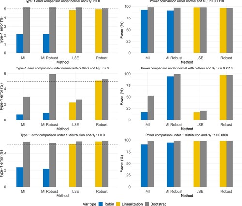
Table (b) and the first two rows of Figure illustrate the simulation results of the original data and the data with extreme outliers under the normal distribution. The observed-only estimator generates a biased ATE estimate as it ignores the information from the dropouts and fails to utilize the J2R imputation model. The no-intermediate estimator also departs from the true value since it lacks using the observed outcomes at intermediate visits and results in a misspecified imputation model. Apart from these two estimators, other methods produced unbiased point estimates when there were no outliers. The robust methods under MI and mean imputation were slightly less efficient compared to MI and LSE, as they had larger MC variances and smaller powers. For MI, Rubin's variance estimates were conservative and inefficient, causing the coverage rates to be far away from the empirical value and the powers to be smaller, which matched the observations in previous literature regarding J2R in longitudinal clinical trials (e.g., G. F. Liu & Pang, Citation2016; S. Liu et al., Citation2022). However, using bootstrap fixed the overestimation issue and produced reasonable coverage rates and power. When outliers existed, only the mean imputation-based robust method produced an unbiased point estimate, a well-controlled type-1 error under , and a satisfying coverage rate under
with a smaller RMSE.
Figure 3. Simulation results under different distributions based on 1000 MC simulations for the methods MI, MI Robust, LSE, and Robust. It visualizes the numerical results in Table and Tables S1–S3 in the supplementary material. The first row shows the type-1 error and power when the outcomes are normally distributed without outliers. The second row presents the results with the incorporation of the outliers in the simulated data. The third row illustrates the results under a heavy-tailed dataset.
6.2. Data from a heavy-tailed distribution
To assess the performance of the estimator from our proposed robust method in heavy-tailed distributions, we generated the longitudinal outcomes sequentially from a -distribution with the degrees of freedom as 5 in time order. Table (c) and the last row of Figure show the simulation results. Similar to Table (b), all methods except the observed-only and no-intermediate methods resulted in unbiased point estimates. The mean imputation-based robust method produced the ATE estimator with the smallest MC variance, indicating the superiority of Huber robust regression under a heavy-tailed distribution. The linearization-based variance estimates behaved similarly to the bootstrap variance estimates for the two mean imputation-based methods, with comparable coverage rates and powers.
6.3. Data under MNAR in the treated group
In the simulations above, the missingness mechanism was set to be MAR in both groups for simplicity. While Assumption 3.1 only imposes missingness ignorability in the control group, we now adjusted the missingness pattern in the active treatment group to MNAR and set the observed probability such that
, where we kept
,
, and
in the control group but set
,
, and
in the active treatment group to get an approximately
missingness rate. Table shows the simulation results under this setting. Apart from the observe-only and no-intermediate methods, all other methods have unbiased estimates when there are no outliers in the data since Assumptions 3.1 and 3.2 are still satisfied. In the presence of extreme outliers, our proposed method has proximal results to the oracle method, showing its superiority in preserving unbiasedness and maintaining satisfying coverage rates.
Table 3. Simulation results under the normal distribution without or with extreme outliers, where the true value and the missingness pattern is MNAR in the treated group.
The overall simulation results supported a recommendation of the proposed robust approach with the linearization-based variance estimation to obtain unbiased point estimates and save computation time. The advocated method worked well in terms of consistency, well-controlled type-1 errors, higher power under , and smaller RMSEs. Even under the normality assumption, our proposed method had comparable performance to MI, with only a slight loss in the power. When encountering a heavy-tailed distribution or extreme outliers, the proposed method outperformed with more reasonable coverage rates and higher powers. Analogous interpretations apply to the simulation results under
given in Section S3.2 of the supplementary material. Moreover, we conducted sensitivity analyses against Assumptions 3.1 and 3.2 to emphasize their importance in Section S3.3 of the supplementary material.
7. Estimating effects of HIV-1 reverse transcriptase inhibitors
We now apply our proposed robust method to the motivating example introduced in Section 2. The primary goal is to assess the ATE between the two arms at the study endpoint in the presence of missing data. The results of the normality test and the symmetry test proposed by Miao et al. (Citation2006) in Figure indicate that the data are symmetrically distributed without severe outliers, yet suffer from a heavy tail that deviates from normality. MI, MI with robust estimators in the analysis step, mean imputation with LS estimators, and the proposed robust method using the Huber loss function are compared with respect to the point estimation, the variance estimation based on Rubin's variance estimator or the linearization-based variance estimator, Wald-type CI and CI length. For MI, the imputation size is M = 100. The tuning parameters for the weights in the robust method are selected via cross-validation, with the procedure described in Section S4 of the supplementary material.
Suppose we believe that the participants no longer enjoy treatment benefits and switch to standard treatment after dropping out of the trial. In that case, J2R offers an attractive assumption to model the missing components. Table shows the analysis results of the group means and the ATE under J2R. The two MI approaches use the sequential LS regressions for the imputation model, resulting in different point estimates compared to other mean imputation-based methods, where the imputation model is obtained via robust regressions. Using LS or Huber loss in the analysis model also slightly differs in the estimation because of the heavy tail in the mean imputation-based methods. While the conventional MI method may contaminate the inference when the data deviates from the normal distribution, the proposed robust method preserves an unbiased estimate and a narrower CI, which coincides with the conclusions drawn from the simulation studies. All the implemented methods show a statistically significant treatment effect under J2R, uncovering the superiority of triple therapies.
Table 4. Analysis of the repeated CD4 count data under J2R.
8. Conclusion
Non-normality frequently occurs in longitudinal clinical trials due to extreme outliers or heavy-tailed errors. With growing attention to evaluating the treatment effect with an MNAR missingness mechanism, we establish a robust method with weighted robust regression and mean imputation under CBI for longitudinal data, without relying on parametric models. Weighted robust regression provides double-layer protection against non-normality in both the covariates and the response variable, ensuring a valid imputation model estimator. Mean imputation and the subsequent robust analysis model further guarantee a valid ATE estimator with good theoretical properties. The proposed method also enjoys the analysis model robustness property, i.e., the consistency and asymptotic normality of the ATE estimator are satisfied even when the analysis model is incorrectly specified.
The symmetrical error distribution, which is an essential assumption in the regression using the robust loss, must be satisfied to obtain a grounded inference for the ATE. However, it may not always be the case in practice. When encountering skewed distributions with asymmetric noise, biases may be detected in our proposed robust method. Takeuchi et al. (Citation2002) provide a novel robust regression method motivated by data mining to handle asymmetric tails and obtain reasonable mean-type estimators. The extension of the proposed robust method may be plausible by replacing the robust regression with their proposed regression model.
While we focus solely on a monotone missingness pattern throughout the development of the robust method, intermittent missingness is also ubiquitous in longitudinal clinical trials. To handle intermittent missing data with a non-ignorable missingness mechanism when the outcomes are non-normal, Elashoff et al. (Citation2012) suggest incorporating the Huber loss function in the pseudo-log-likelihood expression to obtain robust inferences. It is possible to extend our proposed robust method using their idea. We leave it as a future working direction.
Supplemental Material
Download PDF (362.7 KB)Disclosure statement
No potential conflict of interest was reported by the author(s).
Additional information
Funding
References
- Carpenter, J. R., Roger, J. H., & Kenward, M. G. (2013). Analysis of longitudinal trials with protocol deviation: a framework for relevant, accessible assumptions, and inference via multiple imputation. Journal of Biopharmaceutical Statistics, 23(6), 1352–1371. https://doi.org/10.1080/10543406.2013.834911
- Carroll, R. J., & Pederson, S. (1993). On robustness in the logistic regression model. Journal of the Royal Statistical Society. Series B, Statistical Methodology, 55(3), 693–706.
- Chang, L., Roberts, S., & Welsh, A. (2018). Robust lasso regression using Tukey's biweight criterion. Technometrics, 60(1), 36–47. https://doi.org/10.1080/00401706.2017.1305299
- Cro, S., Morris, T. P., Kenward, M. G., & Carpenter, J. R. (2016). Reference-based sensitivity analysis via multiple imputation for longitudinal trials with protocol deviation. The Stata Journal, 16(2), 443–463. https://doi.org/10.1177/1536867X1601600211
- Elashoff, R., Li, G., Li, N., & Tseng, C. H. (2012). Robust inference for longitudinal data analysis with non-ignorable and non-monotonic missing values. Statistics and its Interface, 5(4), 479–490. https://doi.org/10.4310/SII.2012.v5.n4.a11
- Fox, J., & Monette, G. (2002). An R and S-Plus companion to applied regression. Sage.
- Guan, Q., & Yang, S. (2019). A unified framework for causal inference with multiple imputation using martingale. arXiv:1911.04663.
- Henry, K., Erice, A., Tierney, C., Balfour, H. H., Fischl, M. A., Kmack, A., Liou, S. H., Kenton, A., Hirsch, M. S., Phair, J., & Martinez, A. (1998). A randomized, controlled, double-blind study comparing the survival benefit of four different reverse transcriptase inhibitor therapies (three-drug, two-drug, and alternating drug) for the treatment of advanced AIDS. Journal of Acquired Immune Deficiency Syndromes, 19(4), 339–349. https://doi.org/10.1097/00042560-199812010-00004
- Huber, P. J. (1973). Robust regression: Asymptotics, conjectures and Monte Carlo. Annals of Statistics, 1(5), 799–821. https://doi.org/10.1214/aos/1176342503
- Huber, P. J. (2004). Robust statistics (Vol. 523). John Wiley & Sons.
- ICH (2021). E9(R1) statistical principles for clinical trials: Addendum: Estimands and sensitivity analysis in clinical trials. FDA Guidance Documents.
- Jaeckel, L. A. (1972). Estimating regression coefficients by minimizing the dispersion of the residuals. The Annals of Mathematical Statistics, 1449–1458. https://doi.org/10.1214/aoms/1177692377
- Kelly, G. E. (1992). Robust regression estimators-the choice of tuning constans. Journal of the Royal Statistical Society Series D: The Statistician, 41(3), 303–314.
- Leurent, B., Gomes, M., Cro, S., Wiles, N., & Carpenter, J. R. (2020). Reference-based multiple imputation for missing data sensitivity analyses in trial-based cost-effectiveness analysis. Health Economics, 29(2), 171–184. https://doi.org/10.1002/hec.v29.2
- Little, R., & Yau, L. (1996). Intent-to-treat analysis for longitudinal studies with drop-outs. Biometrics, 1324–1333. https://doi.org/10.2307/2532847
- Little, R. J. (1993). Pattern-mixture models for multivariate incomplete data. Journal of the American Statistical Association, 88(421), 125–134.
- Little, R. J., D'Agostino, R., Cohen, M. L., Dickersin, K., Emerson, S. S., Farrar, J. T., Frangakis, C., Hogan, J. W., Molenberghs, G., Murphy, S. A., & Neaton, J. D. (2012). The prevention and treatment of missing data in clinical trials. N Engl J Med, 367(14), 1355–1360. https://doi.org/10.1056/NEJMsr1203730
- Liu, G. F., & Pang, L. (2016). On analysis of longitudinal clinical trials with missing data using reference-based imputation. Journal of Biopharmaceutical Statistics, 26(5), 924–936. https://doi.org/10.1080/10543406.2015.1094810
- Liu, S., Yang, S., Zhang, Y., & Liu, G. F. (2022). Sensitivity analysis in longitudinal clinical trials via distributional imputation. Statistical Methods in Medical Research, 32(1), 181–194. https://doi.org/10.1177/0962280222113525
- Mack, M. J., Leon, M. B., Thourani, V. H., Makkar, R., Kodali, S. K., Russo, M., Kapadia, S. R., Malaisrie, S. C., Cohen, D. J., Pibarot, P., & Leipsic, J. (2019). Transcatheter aortic-valve replacement with a balloon-expandable valve in low-risk patients. N Engl J Med, 380(18), 1695–1705. https://doi.org/10.1056/NEJMoa1814052
- Mallinckrodt, C., Lin, Q., & Molenberghs, M. (2013). A structured framework for assessing sensitivity to missing data assumptions in longitudinal clinical trials. Pharmaceutical Statistics, 12(1), 1–6. https://doi.org/10.1002/pst.1547
- Mehrotra, D. V., Li, X., Liu, J., & Lu, K. (2012). Analysis of longitudinal clinical trials with missing data using multiple imputation in conjunction with robust regression. Biometrics, 68(4), 1250–1259. https://doi.org/10.1111/j.1541-0420.2012.01780.x
- Meyer, G. P. (2021). An alternative probabilistic interpretation of the huber loss. In Proceedings of the IEEE/CVF conference on computer vision and pattern recognition (pp. 5261–5269). IEEE Computer Society.
- Miao, W., Gel, Y. R., & Gastwirth, J. L. (2006). A new test of symmetry about an unknown median. In Random walk, sequential analysis and related topics: A festschrift in honor of Yuan-Shih Chow (pp. 199–214). World Scientific.
- Mogg, R., & Mehrotra, D. V. (2007). Analysis of antiretroviral immunotherapy trials with potentially non-normal and incomplete longitudinal data. Statistics in Medicine, 26(3), 484–497. https://doi.org/10.1002/(ISSN)1097-0258
- O'Neil, P. M., Birkenfeld, A. L., McGowan, B., Mosenzon, O., Pedersen, S. D., Wharton, S., Carson, C. G., Jepsen, C. H., Kabisch, M., & Wilding, J. P. (2018). Efficacy and safety of semaglutide compared with liraglutide and placebo for weight loss in patients with obesity: a randomised, double-blind, placebo and active controlled, dose-ranging, phase 2 trial. The Lancet, 392(10148), 637–649. https://doi.org/10.1016/S0140-6736(18)31773-2
- Ratitch, B., O'Kelly, M., & Tosiello, R. (2013). Missing data in clinical trials: from clinical assumptions to statistical analysis using pattern mixture models. Pharmaceutical Statistics, 12(6), 337–347. https://doi.org/10.1002/pst.1549
- Robins, J. M., & Wang, N. (2000). Inference for imputation estimators. Biometrika, 87(1), 113–124. https://doi.org/10.1093/biomet/87.1.113
- Rosenblum, M., & Van Der Laan, M. J. (2009). Using regression models to analyze randomized trials: Asymptotically valid hypothesis tests despite incorrectly specified models. Biometrics, 65(3), 937–945. https://doi.org/10.1111/j.1541-0420.2008.01177.x
- Rubin, D. B. (1976). Inference and missing data. Biometrika, 63(3), 581–592. https://doi.org/10.1093/biomet/63.3.581
- Rubin, D. B. (2004). Multiple imputation for nonresponse in surveys (Vol. 81). John Wiley & Sons.
- Sadeghkhani, A., Peng, Y., & Lin, C. D. (2019). A parametric Bayesian approach in density ratio estimation. Stats, 2(2), 189–201. https://doi.org/10.3390/stats2020014
- Smola, A. J., & Schölkopf, B. (2004). A tutorial on support vector regression. Statistics and Computing, 14(3), 199–222. https://doi.org/10.1023/B:STCO.0000035301.49549.88
- Sun, Q., Zhou, W. X., & Fan, J. (2020). Adaptive huber regression. Journal of the American Statistical Association, 115(529), 254–265. https://doi.org/10.1080/01621459.2018.1543124
- Takeuchi, I., Bengio, Y., & Kanamori, T. (2002). Robust regression with asymmetric heavy-tail noise distributions. Neural Computation, 14(10), 2469–2496. https://doi.org/10.1162/08997660260293300
- Tan, P. T., Cro, S., Van Vogt, E., Szigeti, M., & Cornelius, V. R. (2021). A review of the use of controlled multiple imputation in randomised controlled trials with missing outcome data. BMC Medical Research Methodology, 21(1), 1–17. https://doi.org/10.1186/s12874-021-01261-6
- Tang, Y. (2017). An efficient multiple imputation algorithm for control-based and delta-adjusted pattern mixture models using SAS. Statistics in Biopharmaceutical Research, 9(1), 116–125. https://doi.org/10.1080/19466315.2016.1225595
- US Food and Drug Administration (2016). Statistical review and evaluation of Tresiba and Ryzodeg 70/30. Retrieved May 26, 2016, from https://www.fda.gov/media/102782/download.
- Yang, S., & Kim, J. K. (2016). A note on multiple imputation for method of moments estimation. Biometrika, 103(1), 244–251. https://doi.org/10.1093/biomet/asv073
- Yang, S., Zhang, Y., Liu, G. F., & Guan, Q. (2021). SMIM: A unified framework of survival sensitivity analysis using multiple imputation and martingale. Biometrics. https://doi.org/10.1111/biom.13555
- Ye, Y., Gao, J., Shao, Y., Li, C., Jin, Y., & Hua, X. (2020). Robust support vector regression with generic quadratic nonconvex ε-insensitive loss. Applied Mathematical Modelling, 82, 235–251. https://doi.org/10.1016/j.apm.2020.01.053