FragmGAN: generative adversarial nets for fragmentary data imputation and prediction

Abstract

Modern scientific research and applications very often encounter ‘fragmentary data’ which brings big challenges to imputation and prediction. By leveraging the structure of response patterns, we propose a unified and flexible framework based on Generative Adversarial Nets (GAN) to deal with fragmentary data imputation and label prediction at the same time. Unlike most of the other generative model based imputation methods that either have no theoretical guarantee or only consider Missing Completed At Random (MCAR), the proposed FragmGAN has theoretical guarantees for imputation with data Missing At Random (MAR) while no hint mechanism is needed. FragmGAN trains a predictor with the generator and discriminator simultaneously. This linkage mechanism shows significant advantages for predictive performances in extensive experiments.

Keywords:

• Data integration
• fragmentary data
• generative adversarial nets
• imputation
• missing at random

1. Introduction

Modern scientific research and applications very often encounter data from multiple data sources, and for each data source, various variables can be collected for data analysis. Such increasing data sources bring big opportunities for predicting people's behaviours with huge potential social and commercial benefits. However, these different data sources usually can not be available for every sample, which leads to ‘fragmentary data’ and brings big challenges to data imputation and label prediction. To be more specific, we introduce two motivating examples that represent the most typically practical scenarios for fragmentary data.

Internet Loan: A leading company of wealth management is exploring its internet loan business and trying to predict the applicants' income for risk management purpose. There are five possibly available data sources (Table 1). (i) Card: the credit card information; (ii) Shopping: the shopping history at internet; (iii) Mobile: the monthly bill of mobile phone; (iv) Bureau: the credit report from the Central Bank; (v) Fraud: the information from an anti-fraud platform. However, some applicants are not willing to provide their shopping or mobile information, not all the applicants have credit reports, and many of them are never included in the database of the anti-fraud platform. As a result, there are 10 ‘response patterns’ in the Internet Loan data as shown in Table 1, where ‘√’ means the data source is available for the applicants with the corresponding response pattern.

Table 1. The response patterns of the Internet Loan data.

Response	Data source
Pattern	Card	Shopping	Mobile	Bureau	Fraud
1	√	√	√	√	√
2	√	√	√	√
3	√	√	√
4	√	√		√	√
5	√	√		√
6	√	√
7	√		√
8	√			√	√
9	√			√
10	√

ADNI: The Alzheimer's Disease Neuroimaging Initiative http://adni.loni.usc.edu is a widely used data by researchers for the Alzheimer's disease which has four data sources. (i) CSF: cerebrospinal fluid; (ii) PET: positron emission tomography; (iii) MRI: magnetic resonance imaging; (iv) Gene: the gene expression. As show in Table 2, it has 8 different response patterns corresponding to different data availability for each data source.

Table 2. The response patterns of the ADNI data.

Response	Data source
Pattern	CSF	PET	MRI	Gene
1	√	√	√	√
2	√	√	√
3	√	√		√
4		√	√	√
5		√		√
6		√	√
7				√
8			√

Such kind of fragmentary data, also known as ‘block-wise missing data’ in the statistics literature, are very common in the area of risk management, marketing research, social sciences, medical studies and so on. Data imputation and label prediction are two main goals for the analysis of such data. But the extremely high missing rate and complicated missing patterns bring big challenges to the achievement of the goals.

Some work has been done to deal with fragmentary data in both areas of statistics and computer sciences in recent years. From the statistics perspective, methods based on model averaging (Fang et al., 2019), factor models (Zhang et al., 2020), generalized methods of moments (Xue & Qu, 2021), iterative least squares (Lin et al., 2021) and integrative factor regression (Li & Li, 2021) are proposed. These statistical methods provide useful theoretical properties but exhibit notable shortcomings. (i) They depend on certain statistical models, for example, linear regression models. (ii) They are not flexible in handling mixed data types that include continuous and categorical variables. (iii) Only a couple of methods consider imputation and prediction at the same time.

From the computer science perspective, GAIN (Yoon et al., 2018) first uses a Generative Adversarial Net (GAN) to impute data Missing Completed At Random (MCAR), which means the missingness occurs entirely at random without depending on any of the variables. MisGAN (Li et al., 2019) trains a mask generator along with the data generator for imputation. GAMIN (Yoon & Sull, 2020) proposes a generative adversarial multiple imputation network for highly missing data. HexaGAN (Hwang et al., 2019) deals with missing data imputation, conditional generation and semi-supervised learning together. GRAPE (You et al., 2020) proposes a graph-based framework for data imputation and label prediction. MIWAE (Mattei & Frellsen, 2019) and Not-MIWAE (Ipsen et al., 2021) propose imputation methods based on variational auto-encoding (VAE) framework instead of GAN. Ma and Chen (2019) proposes a matrix completion algorithm when the data is missing not at random. However, these generative methods have various drawbacks. For instance, some of them (Ipsen et al., 2021; Mattei & Frellsen, 2019; Yoon & Sull, 2020; You et al., 2020) do not have the theoretical guarantee that the imputed data has the same distribution as the original data. Some of them (Hwang et al., 2019; Li et al., 2019; Yoon et al., 2018) only have theoretical results for data MCAR, which is highly unlikely in the practice. Most of them either consider data imputation and label prediction separately or only consider data imputation.

In this paper, by leveraging the structure of response patterns, we propose a ‘FragmGAN’ for fragmentary data imputation and prediction. The main contributions are as follows.

• FragmGAN is a unified framework based on GAN to deal with fragmentary data imputation and label prediction at the same time. It's flexible in the sense that (i) it's applicable to both continuous and categorical data and label, and (ii) users can adjust the relative importance of the task of imputation to prediction by an ‘adjusting factor’.

• FragmGAN has theoretical guarantees for imputation with data Missing At Random (MAR), which is much more general than MCAR and will be defined in Section 3.2. Also, the theoretical results do not need a hint mechanism that is required by GAIN.

• Using similar technical skills, we extend the theoretical results of GAIN to MAR.

• Other than the generator and discriminator, FragmGAN trains a predictor simultaneously. This linkage mechanism shows significant advantages for predictive performances in extensive experiments.

2. Related work

There are lots of discriminative and generative imputation methods that will be considered in our experiments, including Expectation Maximization (García-Laencina et al., 2010), matrix completion (Mazumder et al., 2010), MICE (van Buuren & Groothuis-Oudshoorn, 2011), MissForest (Stekhoven & Buhlmann, 2011) and Auto-Encoder (Gondara & Wang, 2017).

There are several other GAN based imputation methods. CollaGAN (Lee et al., 2019) proposes a collaborative GAN for missing data imputation but it focuses on image data. WGAIN (Friedjungová et al., 2020), CGAIN (Awan et al., 2021), PC-GAIN (Wang et al., 2021) and S-GAIN (Neves et al., 2021) extend GAIN in various ways. IFGAN (Qiu et al., 2020) conducts missing data imputation using a feature-specific GAN and MCFlow (Richardson et al., 2020) proposes a Monte Carlo flow method for data imputation but no theoretical result is provided. When all the variables are assumed to be categorical, theoretical results of GAN based methods are extended to an uncommon concept of Extended Always Missing At Random (Deng et al., 2020).

Although they are not our main interest, we also mention some other VAE based imputation methods including VAEAC (Ivanov et al., 2019), variational inference of deep subspaces (Dalca et al., 2019), iterative imputation using AE dynamics (Smieja et al., 2020), VAE using pattern-set mixtures (Ghalebikesabi et al., 2021) and VSAE (Gong et al., 2021). Some of them only focus on image data. A common disadvantage of VAE based methods is the lack of theoretical guarantee for imputation. Some results of empirical comparison of GAN and VAE based methods are presented in Camino et al. (2019).

3. GAN-Based fragmentary data imputation

We first formulate the problem and discuss the method and theory of fragmentary data imputation in this section. The problem of label prediction will be addressed in Section 4.

Throughout the paper we usually use bold type letters to denote vectors and use the regular letters for scalars. The upper-case letters are used for random variables and the corresponding lower-case letters are their realizations. Abusing notation slightly, we use a generic notation $p(\cdot )$ or $p(\cdot |\cdot )$ to denote the distribution/probability or conditional distribution/probability for various continuous/categorical variables as long as there is no ambiguity.

3.1. Imputation method

Let $\mathbf{X}=(X_1,\dots ,X_d)$ be the d-dimensional data vector of interested variables that could take continuous or categorical values. Note that d is the number of variables but not the number of data sources since each data source may have multiple variables.

Define the mask vector $\mathbf{M}=(M_1,\dots ,M_d)\in \{0,1{\}}^d$ such that $M_i=1$ means $X_i$ is observed and $M_i=0$ means $X_i$ is missing, $i=1,\dots ,d$. So what we actually observe is $\tilde{\mathbf{X}}=\mathbf{M}\odot \mathbf{X}=(M_1{X}_1,\dots ,M_d{X}_d),$where ⊙ denotes element-wise multiplication.

Assume overall there are K (a fixed number) possible response patterns in the data and define $\mathbf{W}=(W_1,\dots ,W_K)$ as the pattern indicator, where $W_k=1$ if the sample belongs to the kth response pattern and $W_k=0$ otherwise, $k=1,\dots ,K$. Note that $\sum _{k=1}^K{W}_k=1$. In the fragmentary data setting, $\mathbf{M}$ can actually only take K (rather than $2^d$) different values and there is a one-to-one mapping between $\mathbf{M}$ and $\mathbf{W}$. In the two motivating examples, K = 10 and 8 respectively.

Generator

Let $\mathbf{Z}=(Z_1,\dots ,Z_d)$ be a d-dimensional noise vector that is independent of all other variables. It is typically taken as Gaussian white noise. We then feed $\tilde{\mathbf{X}}=\mathbf{M}\odot \mathbf{X}$, $\mathbf{Z}$ and $\mathbf{W}$ into the generator G and obtain $\overline{\mathbf{X}}=G(\mathbf{M}\odot \mathbf{X},(1-\mathbf{M})\odot \mathbf{Z},\mathbf{W}),$where G is a function from ${\mathbb{R}}^d\times {\mathbb{R}}^d\times \{{\mathbf{W}}^{\left(1\right)},\dots ,{\mathbf{W}}^{\left(K\right)}\}$ to ${\mathbb{R}}^d$, and $\{{\mathbf{W}}^{\left(1\right)},\dots ,{\mathbf{W}}^{\left(K\right)}\}$ are the K possible values of $\mathbf{W}$. $\overline{\mathbf{X}}$ is the generated data vector but we are only interested in the missing variables. So the complete data vector after imputation is $\hat{\mathbf{X}}=\mathbf{M}\odot \tilde{\mathbf{X}}+(1-\mathbf{M})\odot \overline{\mathbf{X}}=\mathbf{M}\odot \mathbf{X}+(1-\mathbf{M})\odot \overline{\mathbf{X}}.$Our target is to make sure the distribution of $\hat{\mathbf{X}}$ is the same as the distribution of $\mathbf{X}$, i.e., $p\left(\hat{\mathbf{X}}\right)=p\left(\mathbf{X}\right)$. The randomness of $\mathbf{Z}$ makes our method a random imputation method rather than fixed imputation. Although we focus on single imputation in the paper, but by modelling the distribution of the data, we are able to make multiple imputation capture the uncertainty for the imputation value (Rubin, 2004; van Buuren & Groothuis-Oudshoorn, 2011).

Discriminator

The discriminator D tries to figure out which part of $\hat{\mathbf{X}}$ is from the generator. The vanilla GAIN (Yoon et al., 2018) aims to distinguish each component of $\hat{\mathbf{X}}$ is real (observed) or fake (imputed). It's a hard task since d is usually a large number. Consequently, a hint mechanism, which reveals all but one of the components of $\mathbf{M}$ to D, is required for GAIN to solve the model identifiability problem and make sure the generated distribution is what we want.

In the fragmentary data setting, each sample should exactly belong to one of the K response patterns. By leveraging this informative structure, our discriminator D just needs to figure out which pattern $\hat{\mathbf{X}}$ belongs to. So D is a function from ${\mathbb{R}}^d$ to $[0,1{]}^K$ (instead of $[0,1{]}^d$ in GAIN) such that $\hat{\mathbf{W}}=D\left(\hat{\mathbf{X}}\right)=({\hat{W}}_1,\dots ,{\hat{W}}_K)$is the predicted probability vector for $\mathbf{W}$, where ${\hat{W}}_k$ is the predicted probability that $\hat{\mathbf{X}}$ is from the kth response pattern and $\sum _{k=1}^K{\hat{W}}_k=1$. Note that the output layer of D has a softmax form.

We train the discriminator D to maximize the probability of correctly predicting $\mathbf{W}$. On the other hand, the generator G is trained to minimize the probability of D correctly predicting $\mathbf{W}$. The objective function is defined to be the negative cross-entropy loss (1) $V(G,D)={\mathbb{E}}_{(\hat{\mathbf{X}},\mathbf{W})}[\sum _{k=1}^K{W}_k\log D_k(\hat{\mathbf{X}}\left)\right],$(1) where $D_k\left(\hat{\mathbf{X}}\right)$ is just ${\hat{W}}_k$. Note that the objective function depends on G through $\hat{\mathbf{X}}$. Then the minimax problem is given by (2) $\underset{G}{min}\underset{D}{max}V(G,D).$(2)

Remark 3.1

The key difference of our imputation method to GAIN is that we use a different objective function by taking the response patterns into consideration. This adjustment makes sure the model is identifiable even no hint mechanism is used as we show in the next subsection.

3.2. Theoretical results

Most previous theoretical results for GAN-based imputation methods including GAIN (Yoon et al., 2018), MisGAN (Li et al., 2019) and HexaGAN (Hwang et al., 2019) are established under the MCAR assumption, which means the missingness occurs entirely at random without depending on any of the variables. This is a very restrictive assumption and rarely satisfied in the real world. In contrast, our theoretical results will be established under the MAR assumption.

Assume $\mathbf{X}$ can be decomposed into $({\mathbf{X}}^o,{\mathbf{X}}^m)$, where ${\mathbf{X}}^o$ is an always observed subvector of $\mathbf{X}$, and ${\mathbf{X}}^m$ could be missing. The missing mechanism is characterized (Little & Rubin, 2014) into three types.

• Missing Completed At Random (MCAR): $\mathbf{M}$ is independent of $\mathbf{X}$.

• Missing At Random (MAR): $p\left(\mathbf{M}|\mathbf{X}\right)=p\left(\mathbf{M}|{\mathbf{X}}^o\right)$, or equivalently, $\mathbf{M}$ is conditionally independent of ${\mathbf{X}}^m$ given ${\mathbf{X}}^o$.

• Missing Not At Random (MNAR): $p\left(\mathbf{M}|\mathbf{X}\right)$ depends on ${\mathbf{X}}^m$.

Remark 3.2

For a random vector $\mathbf{X}$, it could be ambiguous for the definition of MAR. Another way to define MAR is $p\left(\mathbf{M}|\mathbf{X}\right)=p\left(\mathbf{M}|\right\{X_i:M_i=1,i=1,\dots ,d\left\}\right)$. However, since $\mathbf{M}$ appears in both sides of the condition, there is no way to generate a group of independently and identically distributed samples satisfying this equation, unless there exists an always observed subvector ${\mathbf{X}}^o$ such that $p\left(\mathbf{M}|\mathbf{X}\right)=p\left(\mathbf{M}|{\mathbf{X}}^o\right)$. This is the reason why we use the MAR definition as above.

The complete data vector $\hat{\mathbf{X}}$ can be decomposed into $({\hat{\mathbf{X}}}^o,{\hat{\mathbf{X}}}^m)$ correspondingly. Note that ${\hat{\mathbf{X}}}^o={\mathbf{X}}^o$. So $p\left(\hat{\mathbf{X}}\right)=p\left({\hat{\mathbf{X}}}^o\right)p\left({\hat{\mathbf{X}}}^m|{\hat{\mathbf{X}}}^o\right)=p\left({\mathbf{X}}^o\right)p\left({\hat{\mathbf{X}}}^m|{\mathbf{X}}^o\right).$To verify that the solution to the minimax problem (2(2) $\underset{G}{min}\underset{D}{max}V(G,D).$(2) ) satisfies $p\left(\hat{\mathbf{X}}\right)=p\left(\mathbf{X}\right)$, we just need to show $p\left({\hat{\mathbf{X}}}^m|{\mathbf{X}}^o\right)=p\left({\mathbf{X}}^m|{\mathbf{X}}^o\right)$. First we present a lemma.

Lemma 3.1

Let $\hat{\mathbf{x}}$ is a realization of $\hat{\mathbf{X}}$ such that $p\left(\hat{\mathbf{x}}\right)>0$. For a fixed generator G, the kth component of the optimal discriminator $D^{\ast }\left(\hat{\mathbf{x}}\right)$ to the minimax problem (2(2) $\underset{G}{min}\underset{D}{max}V(G,D).$(2) ) is given by $D_k^{\ast }\left(\hat{\mathbf{x}}\right)=p(\mathbf{W}={\mathbf{w}}_k^0|\hat{\mathbf{x}})$for $k=1,\dots ,K$, where ${\mathbf{w}}_k^0=(0,\dots ,1,\dots ,0)$ is a K-dimensional vector with only the kth element being 1, and $\mathbf{W}={\mathbf{w}}_k^0$ means that the sample belongs to the kth response pattern.

Proof.

All proofs are provided in A.1.

We now rewrite (1(1) $V(G,D)={\mathbb{E}}_{(\hat{\mathbf{X}},\mathbf{W})}[\sum _{k=1}^K{W}_k\log D_k(\hat{\mathbf{X}}\left)\right],$(1) ) by substituting $D^{\ast }$ to obtain the objective function for G to minimize $\begin{array}{rl}C\left(G\right)& =V(D^{\ast },G)\\ & ={\mathbb{E}}_{(\hat{\mathbf{X}},\mathbf{W})}[\sum _{k=1}^K{W}_k\log p(\mathbf{W}={\mathbf{w}}_k^0|\hat{\mathbf{X}}\left)\right].\end{array}$

Theorem 3.2

A global minimum for $C\left(G\right)$ is achieved if and only if (3) $p({\hat{\mathbf{x}}}^m|{\mathbf{x}}^o,\mathbf{W}={\mathbf{w}}_k^0)=p\left({\hat{\mathbf{x}}}^m|{\mathbf{x}}^o\right)$(3) for each $k\in \{1,\dots ,K\}$ and $\hat{\mathbf{x}}=({\mathbf{x}}^o,{\hat{\mathbf{x}}}^m)$ such that $p\left(\hat{\mathbf{x}}\right)>0$ and $p({\mathbf{x}}^o|\mathbf{W}={\mathbf{w}}_k^0)>0$.

It's worthy to mention that Lemma 3.1 and Theorem 3.2 do not depend on the MAR assumption and they are generally true even under MNAR.

Theorem 3.2 tells us that the optimal generator will generate data so that the conditional distributions of ${\hat{\mathbf{X}}}^m$ given ${\mathbf{X}}^o$ across different response patterns are the same. But it does not guarantee $p\left({\hat{\mathbf{X}}}^m|{\mathbf{X}}^o\right)=p\left({\mathbf{X}}^m|{\mathbf{X}}^o\right)$ yet.

To further explore, we assume the first response pattern is the case that all the variables are observed, i.e., $M_i=1$ for all $i\in \{1,\dots ,d\}$. Note the first response patterns in the two motivating examples are exactly the case. Then given $\mathbf{W}={\mathbf{w}}_1^0$, there is no missing variable and we have ${\hat{\mathbf{X}}}^m={\mathbf{X}}^m$. So following (3(3) $p({\hat{\mathbf{x}}}^m|{\mathbf{x}}^o,\mathbf{W}={\mathbf{w}}_k^0)=p\left({\hat{\mathbf{x}}}^m|{\mathbf{x}}^o\right)$(3) ), we have (4) $p\left({\hat{\mathbf{X}}}^m|{\mathbf{X}}^o\right)=p({\hat{\mathbf{X}}}^m|{\mathbf{X}}^o,\mathbf{W}={\mathbf{w}}_1^0)=p({\mathbf{X}}^m|{\mathbf{X}}^o,\mathbf{W}={\mathbf{w}}_1^0).$(4)

Under the MAR assumption, $\mathbf{M}$ is conditionally independent of ${\mathbf{X}}^m$ given ${\mathbf{X}}^o$, and so is $\mathbf{W}$ since there is a one-to-one mapping between $\mathbf{M}$ and $\mathbf{W}$. Therefore (5) $p({\mathbf{X}}^m|{\mathbf{X}}^o,\mathbf{W}={\mathbf{w}}_1^0)=p\left({\mathbf{X}}^m|{\mathbf{X}}^o\right).$(5) Combining (4(4) $p\left({\hat{\mathbf{X}}}^m|{\mathbf{X}}^o\right)=p({\hat{\mathbf{X}}}^m|{\mathbf{X}}^o,\mathbf{W}={\mathbf{w}}_1^0)=p({\mathbf{X}}^m|{\mathbf{X}}^o,\mathbf{W}={\mathbf{w}}_1^0).$(4) ) and (5(5) $p({\mathbf{X}}^m|{\mathbf{X}}^o,\mathbf{W}={\mathbf{w}}_1^0)=p\left({\mathbf{X}}^m|{\mathbf{X}}^o\right).$(5) ) gives us the final theorem that provides theoretical guarantees for our proposed imputation method.

Theorem 3.3

Under the MAR assumption, the density solution to (3(3) $p({\hat{\mathbf{x}}}^m|{\mathbf{x}}^o,\mathbf{W}={\mathbf{w}}_k^0)=p\left({\hat{\mathbf{x}}}^m|{\mathbf{x}}^o\right)$(3) ) is unique and satisfies $p\left({\hat{\mathbf{x}}}^m|{\mathbf{x}}^o\right)=p\left({\mathbf{x}}^m|{\mathbf{x}}^o\right).$So the distribution of $\hat{\mathbf{X}}$ is the same as the distribution of $\mathbf{X}$.

This theorem tells us that the optimal solution is uniquely identified and it is the one we need. Compared to GAIN (Yoon et al., 2018), our method does not need a hint mechanism for model identifiability. An intuitive explanation is that we just need to classify each sample into one of the K response patterns. It requires much fewer model parameters than GAIN, in which d binary classifiers need to be modelled if the hint mechanism is not applied. Note that we only require K to be a fixed number and it could be as large as $2^d$. So theoretically FragmGAN can be applied to any kind of dataset with arbitrary missing patterns when the data vector is low-dimensional, for example, d = 4, and the associated computation is not too heavy. However, FragmGAN is not necessary better than GAIN in such cases. The most suitable scenario for FragmGAN is when K is relatively small compared to $2^d$.

Our theoretical results are established under MAR assumption while the vanilla GAIN (Yoon et al., 2018) assumes MCAR. However, we find that GAIN (with hint) also guarantees that $p\left(\hat{\mathbf{X}}\right)=p\left(\mathbf{X}\right)$ under the MAR assumption, which is consistent to a recent theoretical result (Deng et al., 2020) considering a special case that all the variables are categorical. We provide a direct proof of this conclusion of GAIN in A.2.

4. A unified framework for imputation and prediction

Many previous methods including GAIN (Yoon et al., 2018) consider label prediction as a post-imputation problem, that is, they first impute the data and then develop a prediction model as if the data were fully observed. The disconnection between imputation and prediction mostly likely damages the accuracy of prediction. In this section we propose a unified framework that considers data imputation and label prediction together. The key idea is to train a predictor P with the generator and discriminator simultaneously.

Predictor

Let $\mathbf{Y}$ be the interested q-dimensional label that could be continuous or categorical. Unlike the semi-supervised learning, the label $\mathbf{Y}$ is assumed to be available for all the training samples. A predictor P is a function from ${\mathbb{R}}^d$ to ${\mathbb{R}}^q$ such that $\hat{\mathbf{Y}}=P\left(\hat{\mathbf{X}}\right)$ is a predicted value of $\mathbf{Y}$.

To evaluate the prediction performance of P, we define a loss function $L(\mathbf{Y},P(\hat{\mathbf{X}}\left)\right)$ where L is from ${\mathbb{R}}^d\times {\mathbb{R}}^d$ to $\mathbb{R}$. The explicit form of L depends on the data type of $\mathbf{Y}$ and is very flexible. For example, if $\mathbf{Y}$ is continuous, we may use $L(\mathbf{Y},P(\hat{\mathbf{X}}\left)\right)=\Vert \mathbf{Y}-P\left(\hat{\mathbf{X}}\right){\Vert }^2$. If $\mathbf{Y}\in \{0,1\}$ is a binary scalar and the predicted value is the probability of being 1, then we may use $L(\mathbf{Y},P(\hat{\mathbf{X}}\left)\right)=-\mathbf{Y}\log P\left(\hat{\mathbf{X}}\right)-(1-\mathbf{Y})\log (1-P(\hat{\mathbf{X}}\left)\right)$.

To train G, D and P together, define the linked objective function as (6) $U(G,D,P)=\mathrm{\gamma V}(G,D)+(1-\gamma ){\mathbb{E}}_{(\mathbf{Y},\hat{\mathbf{X}})}L(\mathbf{Y},P(\hat{\mathbf{X}}\left)\right),$(6) where $V(G,D)$ is from (1(1) $V(G,D)={\mathbb{E}}_{(\hat{\mathbf{X}},\mathbf{W})}[\sum _{k=1}^K{W}_k\log D_k(\hat{\mathbf{X}}\left)\right],$(1) ) and $\gamma \in [0,1]$ is an ‘adjusting factor’ that controls the relative importance of data imputation to label prediction.

The second part of (6(6) $U(G,D,P)=\mathrm{\gamma V}(G,D)+(1-\gamma ){\mathbb{E}}_{(\mathbf{Y},\hat{\mathbf{X}})}L(\mathbf{Y},P(\hat{\mathbf{X}}\left)\right),$(6) ) does not involve D, so the target of D is still to maximize $V(G,D)$. The first part of (6(6) $U(G,D,P)=\mathrm{\gamma V}(G,D)+(1-\gamma ){\mathbb{E}}_{(\mathbf{Y},\hat{\mathbf{X}})}L(\mathbf{Y},P(\hat{\mathbf{X}}\left)\right),$(6) ) does not involve P, so the target of P is to minimize the predictive loss ${\mathbb{E}}_{(\mathbf{Y},\hat{\mathbf{X}})}L(\mathbf{Y},P(\hat{\mathbf{X}}\left)\right)$. Both parts of (6(6) $U(G,D,P)=\mathrm{\gamma V}(G,D)+(1-\gamma ){\mathbb{E}}_{(\mathbf{Y},\hat{\mathbf{X}})}L(\mathbf{Y},P(\hat{\mathbf{X}}\left)\right),$(6) ) involve G, but fortunately they both require G to minimize. So the minimax optimization problem is given by (7) $\underset{P}{min}\underset{G}{min}\underset{D}{max}U(G,D,P).$(7)

The choice of γ is quite flexible. If the user is just interested in data imputation, he can take $\gamma =1$ and $U(G,D,P)$ is reduced to $V(G,D)$. If the user is mainly interested in label prediction, he may use a cross-validation procedure to choose an appropriate γ or simply take $\gamma =0.5$ which works quite well as shown in the experiments. Note that $\gamma =0$ is not a good choice since it will lead to overfitting. If the user cares about both imputation and prediction, he may decide γ by the relative importance of the two tasks in his mind.

The pseudo code to implement (7(7) $\underset{P}{min}\underset{G}{min}\underset{D}{max}U(G,D,P).$(7) ) is given in Algorithm 1. Several issues are discussed as follows.

First, although the hint mechanism is not required for our theoretical results, it is still empirically helpful. So we also use the same hint mechanism as Yoon et al. (2018) in implementation. The impact of including the hint mechanism or not will be checked in the experiments.

Second, the generator also generates data even for the observed variables, which can be used to check the generation performance. An extra loss function ${\mathcal{L}}_M:\{0,1{\}}^d\times {\mathbb{R}}^d\times {\mathbb{R}}^d\to \mathbb{R}$ defined as $\alpha \sum _{i=1}^d{M}_i{L}_M({\tilde{X}}_i,{\overline{X}}_i)$ is added to $V(G,D)$ for training G, where $L_M:\mathbb{R}\times \mathbb{R}\to \mathbb{R}$ is a user-specified loss function depending on the variable type of $X_i$. The algorithm result is not sensitive to the choice of hyper-parameter α. Actually, as long as α is relatively large ($\alpha =10$ in the experiments), its main effect is to force ${\overline{X}}_i=X_i$ for the variable with $M_i=1$.

Third, when $\gamma =1$, Algorithm 1 actually implements (2(2) $\underset{G}{min}\underset{D}{max}V(G,D).$(2) ) and the post-imputation prediction.

5. Experiments

In this section we check the imputation and prediction performance of FragmGAN in multiple datasets.

First we consider five UCI datasets (Lichman, 2013) used in GAIN (Yoon et al., 2018): Breast, Spam, Letter, Credit and News. Since the original datasets do not have any missing value, we randomly remove part of data by variable groups to make it fragmentary. Unless otherwise stated, the miss rate is 20%. By designing the removing strategy, we can make it MCAR or MAR. Specifically, we manually set several response patterns in advance. For MCAR, each sample is assigned to the patterns totally at random. For MAR, the probability of each sample being assigned to each pattern depends on the always observed covariate vector ${\mathbf{X}}^o$. For this group of datasets, we are able to check the performance of data imputation along with label prediction since the true data values are known.

Then we consider two datasets Internet Loan and ADNI for the motivating examples introduced in Section 1. The miss rates of them are 46.6% and 22.3%, respectively. More details of these two datasets are provided in A.3. Since the missing values are unknown, we can only check the label prediction performance for these two datasets.

For the purpose of comparison, we consider MICE, MissForest, matrix completion (Matrix), Auto-Encoder (AE), Expectation Maximization (EM) and MisGAN that have been mentioned in Section 1. For the prediction task for Internet Loan and ADNI, we also consider two statistical methods: Model Averaging (Fang et al., 2019) and FR-FI (Zhang et al., 2020).

The hyperparameters of FragmGAN and some implementation details are provided in A.3.

For each dataset, we randomly split it into a training set (80%) and a test set (20%) by response patterns. All the methods are fitted in the training set and then applied to the test set. The imputation and prediction performances are evaluated at the test set. We repeat this experiment 10 times and report the averages and standard deviations of the evaluation criteria (RMSE or AUC). In each table, the best result for each dataset is marked in bold type.

5.1. Results for the UCI datasets

Imputation Performance. Table 3 reports the RMSEs of the imputation errors for the UCI datasets. We take $\gamma =1$ for FragmGAN since imputation is the focus here. For both FragmGAN and GAIN, we consider two versions with or without the hint mechanism.

Table 3. Imputation performance for UCI datasets in terms of RMSE (Average $\pm$ Std) of imputation error.

Algorithm	Breast	Spam	Letter	Credit	News
MCAR, miss rate=20%
FragmGAN	0.0599 $\pm$ .0021	0.0537 $\pm$ .0014	0.1251 $\pm$ .0026	0.1781 $\pm$ .0057	0.1484 $\pm$ .0008
FragmGAN no hint	0.0715 $\pm$ .0022	0.0545 $\pm$ .0007	0.1313 $\pm$ .0078	0.1833 $\pm$ .0020	0.1595 $\pm$ .0049
GAIN	0.0658 $\pm$ .0030	0.0544 $\pm$ .0005	0.1295 $\pm$ .0032	0.1814 $\pm$ .0033	0.1580 $\pm$ .0063
GAIN no hint	0.0736 $\pm$ .0036	0.0574 $\pm$ .0004	0.1338 $\pm$ .0058	0.1899 $\pm$ .0056	0.1606 $\pm$ .0051
MICE	0.0872 $\pm$ .0019	0.0715 $\pm$ .0011	0.1611 $\pm$ .0045	0.1875 $\pm$ .0051	0.2152 $\pm$ .0095
MissForest	0.0608 $\pm$ .0012	0.0594 $\pm$ .0003	0.1371 $\pm$ .0012	0.2033 $\pm$ .0080	0.1932 $\pm$ .0049
Matrix	0.1148 $\pm$ .0021	0.0562 $\pm$ .0012	0.1530 $\pm$ .0035	0.2449 $\pm$ .0033	0.2291 $\pm$ .0061
AE	0.0727 $\pm$ .0011	0.0620 $\pm$ .0007	0.1361 $\pm$ .0020	0.2137 $\pm$ .0026	0.1963 $\pm$ .0004
EM	0.0754 $\pm$ .0027	0.0680 $\pm$ .0002	0.1679 $\pm$ .0005	0.2312 $\pm$ .0008	0.2687 $\pm$ .0003
MisGAN	0.0707 $\pm$ .0016	0.0582 $\pm$ .0004	0.1347 $\pm$ .0020	0.1913 $\pm$ .0008	0.1746 $\pm$ .0034
MAR, miss rate=20%
FragmGAN	0.0667 $\pm$ .0084	0.0512 $\pm$ .0007	0.1364 $\pm$ .0072	0.1844 $\pm$ .0029	0.1630 $\pm$ .0043
FragmGAN no hint	0.0730 $\pm$ .0063	0.0519 $\pm$ .0007	0.1495 $\pm$ .0052	0.1966 $\pm$ .0046	0.1737 $\pm$ .0060
GAIN	0.0671 $\pm$ .0092	0.0526 $\pm$ .0008	0.1457 $\pm$ .0084	0.1909 $\pm$ .0040	0.1690 $\pm$ .0047
GAIN no hint	0.0756 $\pm$ .0099	0.0526$\pm$ 0010	0.1505 $\pm$ .0055	0.1901 $\pm$ .0040	0.1747 $\pm$ .0097
MICE	0.0931 $\pm$ .0060	0.0705 $\pm$ .0008	0.1531 $\pm$ .0059	0.2487 $\pm$ .0078	0.2159 $\pm$ .0096
MissForest	0.0625 $\pm$ .0003	0.0576 $\pm$ .0004	0.1331 $\pm$ .0059	0.2626 $\pm$ .0025	0.1977 $\pm$ .0086
Matrix	0.1146 $\pm$ .0031	0.0556 $\pm$ .0008	0.1488 $\pm$ .0048	0.2268 $\pm$ .0056	0.2337 $\pm$ .0086
AE	0.0843 $\pm$ .0038	0.0618 $\pm$ .0017	0.1427 $\pm$ .0018	0.2110 $\pm$ .0024	0.2048 $\pm$ .0008
EM	0.0869 $\pm$ .0016	0.0678 $\pm$ .0030	0.1784 $\pm$ .0050	0.2412 $\pm$ .0006	0.2659 $\pm$ .0010
MisGAN	0.0713 $\pm$ .0014	0.0577 $\pm$ .0007	0.1428 $\pm$ .0037	0.2014 $\pm$ .0046	0.1883 $\pm$ .0035

As we can see from Table 3, FragmGAN outperforms all the other methods in most cases. For the two cases that FragmGAN is not the best (Breast and Letter with MAR, in which MissForest performs the best), it performs the second best. Both FragmGAN and GAIN perform better than their corresponding versions without hint, indicating that the hint mechanism really helps empirically. This is expected since the hint mechanism provides useful information to the discriminator. Note that the results here can not be directly compared to the results in the paper of GAIN (Yoon et al., 2018) since here we consider fragmentary data with certain response patterns while the missing data in GAIN is generated totally at random.

To check the imputation performance under different miss rates, we take the dataset Credit and generate missing data with miss rate from 10% to 80%. Figure 1 presents the RMSEs of imputation errors under different miss rates. We can see that FragmGAN consistently performs the best. Again, both FragmGAN and GAIN perform better than their corresponding versions without hint. FragmGAN outperforms GAIN in both versions with or without hint.

Figure 1. RMSE of imputation error of the Credit data under different miss rates. Left: MCAR. Right: MAR.

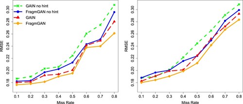
Overall speaking, FragmGAN performs quite well in data imputation in the sense that it has smaller RMSE of imputation error compared to the competitors. Specifically it is better than GAIN, indicating that considering the structure of response patterns in the algorithm is really useful.

Prediction Performance. Table 4 reports the AUCs for the prediction performance in the datasets Breast, Spam, Credit and News. The dataset Letter is not considered here since it does not have a binary label. We include hint for both FragmGAN and GAIN. The adjusting factor γ is taken as 1 or 0.5 for FragmGAN. Note that when $\gamma =1$, FragmGAN first imputes data and then makes the prediction as if the data were fully observed. When $\gamma =0.5$, the imputation and prediction are considered simultaneously.

Table 4. Prediction performance for UCI datasets in terms of AUC (Average ± Std).

Algorithm	Breast	Spam	Credit	News
MCAR, miss rate=20%
FragmGAN $\gamma =0.5$	0.9932 ± .0035	0.9534 ± .0029	0.7643 ± .0034	0.9709 ± .0020
FragmGAN $\gamma =1$	0.9920 ± .0056	0.9528 ± .0030	0.7557 ± .0021	0.9620 ± .0017
GAIN	0.9912 ± .0055	0.9513 ± .0037	0.7521 ± .0022	0.9607 ± .0026
MICE	0.9809 ± .0045	0.9444 ± .0032	0.7492 ± .0038	0.9294 ± .0021
MissForest	0.9892 ± .0060	0.9466 ± .0069	0.7495 ± .0026	0.9409 ± .0029
Matrix	0.9827 ± .0062	0.9021 ± .0057	0.7273 ± .0074	0.8438 ± .0054
AE	0.9850 ± .0078	0.9392 ± .0053	0.7463 ± .0044	0.9211 ± .0025
EM	0.9853 ± .0029	0.9172 ± .0059	0.7418 ± .0068	0.8754 ± .0028
MisGAN	0.9858 ± .0025	0.9485 ± .0042	0.7488 ± .0017	0.9505 ± .0012
MAR, miss rate=20%
FragmGAN $\gamma =0.5$	0.9936 ± .0056	0.9530 ± .0034	0.7622 ± .0027	0.9696 ± .0024
FragmGAN $\gamma =1$	0.9928 ± .0045	0.9521 ± .0029	0.7518 ± .0015	0.9598 ± .0017
GAIN	0.9914 ± .0040	0.9511 ± .0032	0.7505 ± .0021	0.9592 ± .0023
MICE	0.9878 ± .0063	0.9375 ± .0036	0.7366 ± .0033	0.9325 ± .0040
MissForest	0.9839 ± .0035	0.9519 ± .0042	0.7355 ± .0026	0.9405 ± .0026
Matrix	0.9815 ± .0083	0.9033 ± .0045	0.7342 ± .0028	0.8596 ± .0036
AE	0.9895 ± .0056	0.9347 ± .0041	0.7485 ± .0056	0.9291 ± .0041
EM	0.9892 ± .0064	0.9134 ± .0036	0.7427 ± .0063	0.8828 ± .0061
MisGAN	0.9863 ± .0023	0.9499 ± .0050	0.7483 ± .0021	0.9492 ± .0020

As we can see, FragmGAN with $\gamma =0.5$ outperforms the other methods in all the cases. This result shows that the linkage mechanism of training generator and predictor together can improve the prediction performance as we expected. Also note that although FragmGAN with $\gamma =1$ performs worse than FragmGAN with $\gamma =0.5$, it still performs better than all the other methods.

5.2. Results for the motivating examples

For the dataset Internet Loan, the original label is the applicant's income, which is a continuous variable. In the analysis we use $\log \left(\mathrm{income}\right)$ as the label Y. For the dataset ADNI, the original label Y is the score of Mini-Mental State Examination (MMSE) taking value from 0 to 30, in which higher score means better cognitive function. In the real analysis, we consider two labels. (i) The normalized MMSE which can be considered as a continuous variable. (ii) A binary label Y = 1 if MMSE≥28 and Y = 0 otherwise.

Prediction Performance. Table 5 reports the RMSEs for the continuous label prediction and AUCs for the binary label prediction. The last two methods (Model Averaging and FR-FI) rely on linear regression models so they are not applicable to the binary label prediction. For the proposed FragmGAN, we take $\gamma =$1, 0.75, 0.5 and 0.25, indicating different relative importance of imputation to prediction. Also, we use a 5-fold cross-validation to select the best (for label prediction) γ. The CV criterion is defined as the averaged prediction performance in the leave-out samples.

Table 5. Prediction performance for the two motivation examples (Average ± Std).

Algorithm	Internet Loan (RMSE)	ADNI (RMSE)	ADNI (AUC)
FragmGAN ${\gamma }_{\mathrm{cv}}$	0.8865 ± .0015	0.0851 ± .0019	0.7823 ± .0026
FragmGAN $\gamma =1$	0.9267 ± .0036	0.0897 ± .0022	0.7701 ± .0036
FragmGAN $\gamma =0.75$	0.9151 ± .0029	0.0883 ± .0023	0.7721 ± .0028
FragmGAN $\gamma =0.5$	0.8928 ± .0026	0.0871 ± .0020	0.7773 ± .0023
FragmGAN $\gamma =0.25$	0.9286 ± .0044	0.0895 ± .0028	0.7719 ± .0018
GAIN	0.9246 ± .0034	0.0921 ± .0014	0.7622 ± .0028
MICE	0.9934 ± .0036	0.1034 ± .0029	0.6587 ± .0029
MissForest	0.9982 ± .0041	0.1124 ± .0019	0.7583 ± .0022
Matrix	0.9913 ± .0039	0.1134 ± .0016	0.7343 ± .0018
AE	0.9884 ± .0035	0.0994 ± .0017	0.7400 ± .0036
EM	0.9896 ± .0034	0.1042 ± .0023	0.7020 ± .0048
MisGAN	0.9889 ± .0021	0.0997 ± .0024	0.7384 ± .0026
Model Averaging	0.9831 ± .0071	0.1000 ± .0095	not applicable
FR-FI	1.0560 ± .0112	0.1057 ± .0087	not applicable

Table 5 shows that FragmGAN with the ${\gamma }_{\mathrm{cv}}$ selected by cross-validation outperforms all the other methods in all the three cases, indicating that cross-validation is a good way to choose γ. FragmGAN with $\gamma =0.5$ always performs the second best. Note that γ controls the relative importance of data imputation to label prediction. As γ decreases from 1 to 0.25, the prediction performances first increase and then decrease. This result confirms two points that we have made: first, the linkage mechanism of training generator and predictor together can improve the prediction performance; second, a small γ close to 0 will lead to overfitting and damage the label prediction performance at the test data. Base on the results, we believe $\gamma =0.5$ is a reasonable choice if the users are not willing to apply cross validation to choose the best γ due to the computational burden.

6. Concluding remarks

Fragmentary data is becoming more and more popular in many areas and it is not easy to handle. By leveraging the structure in the response patterns, we propose a unified and flexible GAN based framework to deal with data imputation and label prediction simultaneously. An adjusting factor γ is used to adjust the relative importance of imputation to prediction. Theoretical guarantees for imputation are provided under the MAR assumption. Extensive experiments confirm the superiority of our proposed FragmGAN. It has wide application prospects especially in personal internet credit investigation, individual patient data (IPD) meta analysis in medical research and so on.

Based on the theoretical explorations and results of the experiments, we provide several practical suggestions for implementing FragmGAN in the practice.

• Always use the hint mechanism although it is not required for the theoretical results.

• Use $\gamma =1$ if there is no label in the analysis or you are only interested in data imputation.

• If you are interested in label prediction, use cross-validation to select the best γ or simply use $\gamma =0.5$.

Possible future work includes the following. (i) We find that the best performances of data imputation (requires $\gamma =1$) and label prediction (requires a γ between 0 and 1) are not achieved at the same time. This is an interesting phenomenon and further investigation may lead to some thought-provoking results. (ii) In this paper we assume that the label is always available in the training data. We may explore FragmGAN under a semi-supervised setting in which some labels are not available. A naive method is to consider the label as part of the data vector and apply GAIN or FragmGAN directly. But this method is trying to recover the distribution of $\mathbf{X}$ and the conditional distribution of $\mathbf{Y}|\mathbf{X}$, which may not be desirable as we just mentioned in the first point. (iii) In this paper we assume that data are MAR. The extension of the results to the more general case of MNAR is a difficult but interesting task.

Disclosure statement

No potential conflict of interest was reported by the author(s).

Additional information

Funding

The authors gratefully acknowledge the research support from the National Key R&D Program of China [Grant Numbers 2021YFA1000100 and 2021YFA1000101], National Natural Science Foundation of China [Grant Numbers 72331005, 12071143 and 11831008] and the Basic Research Project of Shanghai Science and Technology Commission [Grant Number 22JC1400800].

Appendices

Appendix 1.

A.1. Proofs of the proposed FragmGAN

1.1. Proof of Lemma 3.1

Proof.

Let ${\pi }_k=P(\mathbf{W}={\mathbf{w}}_k^0)$. (A1) $\begin{array}{rl}V(G,D)& ={\mathbb{E}}_{(\hat{\mathbf{X}},\mathbf{W})}[\sum _{k=1}^K{W}_k\log D_k(\hat{\mathbf{X}}\left)\right]\\ & =\sum _{k=1}^{K}P(\mathbf{W}={\mathbf{w}}_k^0){\int }_{\hat{\mathbf{x}}}p(\hat{\mathbf{x}}|\mathbf{W}={\mathbf{w}}_k^0)\log D_k\left(\hat{\mathbf{x}}\right)\mathrm{d}\hat{\mathbf{x}}\\ & ={\int }_{\hat{\mathbf{x}}}\left[\sum _{k=1}^K{\pi }_{k}p\right(\hat{\mathbf{x}}|\mathbf{W}={\mathbf{w}}_k^0)\log D_k(\hat{\mathbf{x}}\left)\right]\mathrm{d}\hat{\mathbf{x}}.\end{array}$(A1) Note that $\sum _{k=1}^K{D}_k\left(\hat{\mathbf{x}}\right)=1$. By the fact that $\sum _{k=1}^K{c}_k\log x_k$ with $\sum _{k=1}^K{x}_k=1$ achieving its maximum when $x_k=\frac{c_k}{\sum _{k=1}^K{c}_k}$, (A1(A1) $\begin{array}{rl}V(G,D)& ={\mathbb{E}}_{(\hat{\mathbf{X}},\mathbf{W})}[\sum _{k=1}^K{W}_k\log D_k(\hat{\mathbf{X}}\left)\right]\\ & =\sum _{k=1}^{K}P(\mathbf{W}={\mathbf{w}}_k^0){\int }_{\hat{\mathbf{x}}}p(\hat{\mathbf{x}}|\mathbf{W}={\mathbf{w}}_k^0)\log D_k\left(\hat{\mathbf{x}}\right)\mathrm{d}\hat{\mathbf{x}}\\ & ={\int }_{\hat{\mathbf{x}}}\left[\sum _{k=1}^K{\pi }_{k}p\right(\hat{\mathbf{x}}|\mathbf{W}={\mathbf{w}}_k^0)\log D_k(\hat{\mathbf{x}}\left)\right]\mathrm{d}\hat{\mathbf{x}}.\end{array}$(A1) ) is maximized (for fixed G) when $D_k\left(\hat{\mathbf{x}}\right)=\frac{{\pi }_{k}p(\hat{\mathbf{x}}|\mathbf{W}={\mathbf{w}}_k^0)}{\sum _{k=1}^K{\pi }_{k}p(\hat{\mathbf{x}}|\mathbf{W}={\mathbf{w}}_k^0)}=p(\mathbf{W}={\mathbf{w}}_k^0|\hat{\mathbf{x}}):=D_k^{\ast }\left(\hat{\mathbf{x}}\right)$for the $\hat{\mathbf{x}}$ such that $p\left(\hat{\mathbf{x}}\right)>0$.

1.2. Proof of Theorem 3.2

Proof.

(A2) $\begin{array}{rl}C\left(G\right)& =V(D^{\ast },G)\\ & ={\mathbb{E}}_{(\hat{\mathbf{X}},\mathbf{W})}[\sum _{k=1}^K{W}_k\log p(\mathbf{W}={\mathbf{w}}_k^0|\hat{\mathbf{X}}\left)\right]\\ & =\sum _{k=1}^K{\pi }_k{\int }_{\hat{\mathbf{x}}}p(\hat{\mathbf{x}}|\mathbf{W}={\mathbf{w}}_k^0)\log p(\mathbf{W}={\mathbf{w}}_k^0|\hat{\mathbf{x}})\mathrm{d}\hat{\mathbf{x}}\\ & =\sum _{k=1}^K{\pi }_k{\int }_{\hat{\mathbf{x}}}p(\hat{\mathbf{x}}|\mathbf{W}={\mathbf{w}}_k^0)\log \frac{p(\hat{\mathbf{x}}|\mathbf{W}={\mathbf{w}}_k^0){\pi }_k}{p\left(\hat{\mathbf{x}}\right)}\mathrm{d}\hat{\mathbf{x}}\\ & =\sum _{k=1}^K{\pi }_k{\int }_{\hat{\mathbf{x}}}p(\hat{\mathbf{x}}|\mathbf{W}={\mathbf{w}}_k^0)\log \frac{p(\hat{\mathbf{x}}|\mathbf{W}={\mathbf{w}}_k^0)}{p\left(\hat{\mathbf{x}}\right)}\mathrm{d}\hat{\mathbf{x}}+\sum _{k=1}^K{\pi }_k{\int }_{\hat{\mathbf{x}}}p(\hat{\mathbf{x}}|\mathbf{W}={\mathbf{w}}_k^0)\log {\pi }_k\mathrm{d}\hat{\mathbf{x}}\\ & \propto \sum _{k=1}^K{\pi }_k{\int }_{\hat{\mathbf{x}}}p({\hat{\mathbf{x}}}^m|{\mathbf{x}}^o,\mathbf{W}={\mathbf{w}}_k^0)p({\mathbf{x}}^o|\mathbf{W}={\mathbf{w}}_k^0)\log \frac{p({\hat{\mathbf{x}}}^m|{\mathbf{x}}^o,\mathbf{W}={\mathbf{w}}_k^0)p({\mathbf{x}}^o|\mathbf{W}={\mathbf{w}}_k^0)}{p\left({\hat{\mathbf{x}}}^m|{\mathbf{x}}^o\right)p\left({\mathbf{x}}^o\right)}\mathrm{d}\hat{\mathbf{x}}\end{array}$(A2) (A3) $\begin{array}{rl}& =\sum _{k=1}^K{\pi }_k{\int }_{{\mathbf{x}}^o}p({\mathbf{x}}^o|\mathbf{W}={\mathbf{w}}_k^0)\left[{\int }_{{\hat{\mathbf{x}}}^m}p\right({\hat{\mathbf{x}}}_m|{\mathbf{x}}^o,\mathbf{W}={\mathbf{w}}_k^0)\log \frac{p({\hat{\mathbf{x}}}^m|{\mathbf{x}}^o,\mathbf{W}={\mathbf{w}}_k^0)}{p\left({\hat{\mathbf{x}}}^m|{\mathbf{x}}^o\right)}\mathrm{d}{\hat{\mathbf{x}}}^m]\mathrm{d}{\mathbf{x}}^o\\ & +\sum _{k=1}^K{\pi }_k{\int }_{{\mathbf{x}}^o}p({\mathbf{x}}^o|\mathbf{W}={\mathbf{w}}_k^0)\left[{\int }_{{\hat{\mathbf{x}}}^m}p\right({\hat{\mathbf{x}}}_m|{\mathbf{x}}^o,\mathbf{W}={\mathbf{w}}_k^0)\log \frac{p({\mathbf{x}}^o|\mathbf{W}={\mathbf{w}}_k^0)}{p\left({\mathbf{x}}^o\right)}\mathrm{d}{\hat{\mathbf{x}}}^m]\mathrm{d}{\mathbf{x}}^o,\end{array}$(A3) where ‘∝’ means equation holds by ignoring terms unrelated to G, and (A2(A2) $\begin{array}{rl}C\left(G\right)& =V(D^{\ast },G)\\ & ={\mathbb{E}}_{(\hat{\mathbf{X}},\mathbf{W})}[\sum _{k=1}^K{W}_k\log p(\mathbf{W}={\mathbf{w}}_k^0|\hat{\mathbf{X}}\left)\right]\\ & =\sum _{k=1}^K{\pi }_k{\int }_{\hat{\mathbf{x}}}p(\hat{\mathbf{x}}|\mathbf{W}={\mathbf{w}}_k^0)\log p(\mathbf{W}={\mathbf{w}}_k^0|\hat{\mathbf{x}})\mathrm{d}\hat{\mathbf{x}}\\ & =\sum _{k=1}^K{\pi }_k{\int }_{\hat{\mathbf{x}}}p(\hat{\mathbf{x}}|\mathbf{W}={\mathbf{w}}_k^0)\log \frac{p(\hat{\mathbf{x}}|\mathbf{W}={\mathbf{w}}_k^0){\pi }_k}{p\left(\hat{\mathbf{x}}\right)}\mathrm{d}\hat{\mathbf{x}}\\ & =\sum _{k=1}^K{\pi }_k{\int }_{\hat{\mathbf{x}}}p(\hat{\mathbf{x}}|\mathbf{W}={\mathbf{w}}_k^0)\log \frac{p(\hat{\mathbf{x}}|\mathbf{W}={\mathbf{w}}_k^0)}{p\left(\hat{\mathbf{x}}\right)}\mathrm{d}\hat{\mathbf{x}}+\sum _{k=1}^K{\pi }_k{\int }_{\hat{\mathbf{x}}}p(\hat{\mathbf{x}}|\mathbf{W}={\mathbf{w}}_k^0)\log {\pi }_k\mathrm{d}\hat{\mathbf{x}}\\ & \propto \sum _{k=1}^K{\pi }_k{\int }_{\hat{\mathbf{x}}}p({\hat{\mathbf{x}}}^m|{\mathbf{x}}^o,\mathbf{W}={\mathbf{w}}_k^0)p({\mathbf{x}}^o|\mathbf{W}={\mathbf{w}}_k^0)\log \frac{p({\hat{\mathbf{x}}}^m|{\mathbf{x}}^o,\mathbf{W}={\mathbf{w}}_k^0)p({\mathbf{x}}^o|\mathbf{W}={\mathbf{w}}_k^0)}{p\left({\hat{\mathbf{x}}}^m|{\mathbf{x}}^o\right)p\left({\mathbf{x}}^o\right)}\mathrm{d}\hat{\mathbf{x}}\end{array}$(A2) ) holds since ${\int }_{\hat{\mathbf{x}}}p(\hat{\mathbf{x}}|\mathbf{W}={\mathbf{w}}_k^0)\mathrm{d}\hat{\mathbf{x}}=1$ is a constant and $\hat{\mathbf{x}}=({\mathbf{x}}^o,{\hat{\mathbf{x}}}^m)$. Note that $\log \frac{p({\mathbf{x}}^o|\mathbf{W}={\mathbf{w}}_k^o)}{p\left({\mathbf{x}}^o\right)}$ is unrelated to ${\hat{\mathbf{x}}}^m$ and ${\int }_{{\hat{\mathbf{x}}}^m}p({\hat{\mathbf{x}}}^m|{\mathbf{x}}^o,\mathbf{W}={\mathbf{w}}_k^0)\mathrm{d}{\hat{\mathbf{x}}}^m=1$, so the second term of (A3(A3) $\begin{array}{rl}& =\sum _{k=1}^K{\pi }_k{\int }_{{\mathbf{x}}^o}p({\mathbf{x}}^o|\mathbf{W}={\mathbf{w}}_k^0)\left[{\int }_{{\hat{\mathbf{x}}}^m}p\right({\hat{\mathbf{x}}}_m|{\mathbf{x}}^o,\mathbf{W}={\mathbf{w}}_k^0)\log \frac{p({\hat{\mathbf{x}}}^m|{\mathbf{x}}^o,\mathbf{W}={\mathbf{w}}_k^0)}{p\left({\hat{\mathbf{x}}}^m|{\mathbf{x}}^o\right)}\mathrm{d}{\hat{\mathbf{x}}}^m]\mathrm{d}{\mathbf{x}}^o\\ & +\sum _{k=1}^K{\pi }_k{\int }_{{\mathbf{x}}^o}p({\mathbf{x}}^o|\mathbf{W}={\mathbf{w}}_k^0)\left[{\int }_{{\hat{\mathbf{x}}}^m}p\right({\hat{\mathbf{x}}}_m|{\mathbf{x}}^o,\mathbf{W}={\mathbf{w}}_k^0)\log \frac{p({\mathbf{x}}^o|\mathbf{W}={\mathbf{w}}_k^0)}{p\left({\mathbf{x}}^o\right)}\mathrm{d}{\hat{\mathbf{x}}}^m]\mathrm{d}{\mathbf{x}}^o,\end{array}$(A3) ) is unrelated to G. Following (A3(A3) $\begin{array}{rl}& =\sum _{k=1}^K{\pi }_k{\int }_{{\mathbf{x}}^o}p({\mathbf{x}}^o|\mathbf{W}={\mathbf{w}}_k^0)\left[{\int }_{{\hat{\mathbf{x}}}^m}p\right({\hat{\mathbf{x}}}_m|{\mathbf{x}}^o,\mathbf{W}={\mathbf{w}}_k^0)\log \frac{p({\hat{\mathbf{x}}}^m|{\mathbf{x}}^o,\mathbf{W}={\mathbf{w}}_k^0)}{p\left({\hat{\mathbf{x}}}^m|{\mathbf{x}}^o\right)}\mathrm{d}{\hat{\mathbf{x}}}^m]\mathrm{d}{\mathbf{x}}^o\\ & +\sum _{k=1}^K{\pi }_k{\int }_{{\mathbf{x}}^o}p({\mathbf{x}}^o|\mathbf{W}={\mathbf{w}}_k^0)\left[{\int }_{{\hat{\mathbf{x}}}^m}p\right({\hat{\mathbf{x}}}_m|{\mathbf{x}}^o,\mathbf{W}={\mathbf{w}}_k^0)\log \frac{p({\mathbf{x}}^o|\mathbf{W}={\mathbf{w}}_k^0)}{p\left({\mathbf{x}}^o\right)}\mathrm{d}{\hat{\mathbf{x}}}^m]\mathrm{d}{\mathbf{x}}^o,\end{array}$(A3) ), we have $C\left(G\right)\propto \sum _{k=1}^K{\pi }_k{\int }_{{\mathbf{x}}^o}p({\mathbf{x}}^o|\mathbf{W}={\mathbf{w}}_k^0)\text{KL}(p({\hat{\mathbf{x}}}^m|{\mathbf{x}}^o,\mathbf{W}={\mathbf{w}}_k^0)||p\left({\hat{\mathbf{x}}}^m|{\mathbf{x}}^o\right))\mathrm{d}{\mathbf{x}}^o,$where KL$(\cdot ||\cdot )$ denotes the KL divergence. Its minimum is achieved when $p({\hat{\mathbf{x}}}^m|{\mathbf{x}}^o,\mathbf{W}={\mathbf{w}}_k^0)=p\left({\hat{\mathbf{x}}}^m|{\mathbf{x}}^o\right)$ for each $k\in \{1,\dots ,K\}$ and (almost) every $\mathbf{x}$ such that $p\left(\hat{\mathbf{x}}\right)>0$ and $p({\mathbf{x}}^o|\mathbf{W}={\mathbf{w}}_k^0)>0$.

1.3. Proof of Theorem 3.3

Proof.

Actually we have proved this theorem in the statements between Theorem 3.2 and Theorem 3.3 in Section 3.2.

A.2. Extend theoretical results of GAIN (Yoon et al., 2018) to missing at random

We first rewrite the formulation of GAIN under MAR with our notation (just a little bit different from the original GAIN paper).

The original data $\mathbf{X}=({\mathbf{X}}^o,{\mathbf{X}}^m)\in {\mathbb{R}}^d$, dim$\left({\mathbf{X}}^o\right)=d^o$, dim$\left({\mathbf{X}}^m\right)=d^m$ and $d^o+d^m=d$. Denote $\mathbf{M}\in \{0,1{\}}^{d^m}$ as the response indicator for ${\mathbf{X}}^m$. We assume ${\mathbf{X}}^m$ is missing at random, i.e., $p\left(\mathbf{M}|\mathbf{X}\right)=p\left(\mathbf{M}|{\mathbf{X}}^o\right)$. Let $\mathbf{Z}=(Z_1,\dots ,Z_{d^m})$ be a $d^m$-dimensional noise vector. Denote $\begin{array}{rl}{\overline{\mathbf{X}}}^m& =G({\mathbf{X}}^o,\mathbf{M}\odot {\mathbf{X}}^m,(1-\mathbf{M})\odot \mathbf{Z},\mathbf{M})\in {\mathbb{R}}^{d^m},\\ {\hat{\mathbf{X}}}^m& =\mathbf{M}\odot {\mathbf{X}}^m+(1-\mathbf{M})\odot {\overline{\mathbf{X}}}^m\in {\mathbb{R}}^{d^m},\end{array}$and $\hat{\mathbf{X}}=({\mathbf{X}}^o,{\hat{\mathbf{X}}}^m)\in {\mathbb{R}}^d$ is the complete data after imputation. Let $\mathbf{H}\in {\mathbb{R}}^{d^m}$ be the hint vector. The discriminator D is a function from ${\mathbb{R}}^d\times {\mathbb{R}}^{d^m}$ to $[0,1{]}^{d^m}$ such that $\hat{\mathbf{M}}=D(\hat{\mathbf{X}},\mathbf{H})=({\hat{M}}_1,\dots ,{\hat{M}}_{d_m})$is the predicted probability vector for $\mathbf{M}$. The minimax problem is (A4) $\underset{G}{min}\underset{D}{max}V(G,D)=\underset{G}{min}\underset{D}{max}{\mathbb{E}}_{(\hat{\mathbf{X}},\mathbf{M},\mathbf{H})}[{\mathbf{M}}^{\mathrm{\top }}\log D(\hat{\mathbf{X}},\mathbf{H})+(1-\mathbf{M}{)}^{\mathrm{\top }}\log (1-D(\hat{\mathbf{X}},\mathbf{H}\left)\right)],$(A4) where log is element-wise logarithm and dependence on G is through $\hat{\mathbf{X}}$.

The proof of Lemma 1 in GAIN (Yoon et al., 2018) does not depend on the decomposition of $\mathbf{X}$. So the result still holds: the optimal D for given G is given by $D_i^{\ast }(\hat{\mathbf{x}},\mathbf{h})=p(M_i=1|\hat{\mathbf{x}},\mathbf{h})$for $i\in \{1,\dots ,d^m\}$.

Denote ${\mathcal{H}}_t^i=\{\mathbf{h}:p(\mathbf{h}|m_i=t)>0\}$ for $t\in \{0,1\}$ and $i\in \{1,\dots ,d^m\}$. Substituting $D^{\ast }=(D_1^{\ast },\dots ,D_{d^m}^{\ast })$ into $V(G,D)$ in (A4(A4) $\underset{G}{min}\underset{D}{max}V(G,D)=\underset{G}{min}\underset{D}{max}{\mathbb{E}}_{(\hat{\mathbf{X}},\mathbf{M},\mathbf{H})}[{\mathbf{M}}^{\mathrm{\top }}\log D(\hat{\mathbf{X}},\mathbf{H})+(1-\mathbf{M}{)}^{\mathrm{\top }}\log (1-D(\hat{\mathbf{X}},\mathbf{H}\left)\right)],$(A4) ), we have the objective function for G (to minimize): (A5) $\begin{array}{rl}C\left(G\right)& ={\mathbb{E}}_{(\hat{\mathbf{X}},\mathbf{M},\mathbf{H})}[\sum _{i:M_i=1}\log p(m_i=1|\hat{\mathbf{X}},\mathbf{H})+\sum _{i:M_i=0}\log p(m_i=0|\hat{\mathbf{X}},\mathbf{H}\left)\right]\\ & ={\int }_{\hat{\mathbf{x}}}{\int }_{\mathbf{h}}\sum _{i=1}^{d^m}\left[p\right(\hat{\mathbf{x}},\mathbf{h},m_i=1)\log p(m_i=1|\hat{\mathbf{x}},\mathbf{h})+p(\hat{\mathbf{x}},\mathbf{h},m_i=0)\log p(m_i=0|\hat{\mathbf{x}},\mathbf{h}\left)\right]\mathrm{d}\mathbf{h}\mathrm{d}\hat{\mathbf{x}}\\ & =\sum _{i=1}^{d_m}\sum _{t\in \{0,1\}}{\int }_{{\mathcal{H}}_t^i}{\int }_{\hat{\mathbf{x}}}p(\hat{\mathbf{x}},\mathbf{h},m_i=t)\log p(m_i=t|\hat{\mathbf{x}},\mathbf{h})\mathrm{d}\mathbf{h}\mathrm{d}\hat{\mathbf{x}}\\ & =\sum _{i=1}^{d_m}\sum _{t\in \{0,1\}}{\int }_{{\mathcal{H}}_t^i}{\int }_{\hat{\mathbf{x}}}p(\hat{\mathbf{x}},\mathbf{h},m_i=t)\log \frac{p(\hat{\mathbf{x}},m_i=t|\mathbf{h})}{p\left(\hat{\mathbf{x}}|\mathbf{h}\right)}\mathrm{d}\mathbf{h}\mathrm{d}\hat{\mathbf{x}}\\ & =\sum _{i=1}^{d_m}\sum _{t\in \{0,1\}}{\int }_{{\mathcal{H}}_t^i}{\int }_{\hat{\mathbf{x}}}p(\hat{\mathbf{x}},\mathbf{h},m_i=t)\log \frac{p(\hat{\mathbf{x}},m_i=t|\mathbf{h})p(m_i=t|\mathbf{h})}{p\left(\hat{\mathbf{x}}|\mathbf{h}\right)p(m_i=t|\mathbf{h})}\mathrm{d}\mathbf{h}\mathrm{d}\hat{\mathbf{x}}\\ & =\sum _{i=1}^{d_m}\sum _{t\in \{0,1\}}{\int }_{{\mathcal{H}}_t^i}{\int }_{\hat{\mathbf{x}}}p(\hat{\mathbf{x}},\mathbf{h},m_i=t)\log \frac{p(\hat{\mathbf{x}}|\mathbf{h},m_i=t)p(m_i=t|\mathbf{h})}{p\left(\hat{\mathbf{x}}|\mathbf{h}\right)}\mathrm{d}\mathbf{h}\mathrm{d}\hat{\mathbf{x}}\\ & =\sum _{i=1}^{d_m}\sum _{t\in \{0,1\}}{\int }_{{\mathcal{H}}_t^i}{\int }_{\hat{\mathbf{x}}}p(\hat{\mathbf{x}},\mathbf{h},m_i=t)\log \frac{p(\hat{\mathbf{x}}|\mathbf{h},m_i=t)}{p\left(\hat{\mathbf{x}}|\mathbf{h}\right)}\mathrm{d}\mathbf{h}\mathrm{d}\hat{\mathbf{x}}\\ & +\sum _{i=1}^{d_m}\sum _{t\in \{0,1\}}{\int }_{{\mathcal{H}}_t^i}{\int }_{\hat{\mathbf{x}}}p(\hat{\mathbf{x}},\mathbf{h},m_i=t)\log p(m_i=t|\mathbf{h})\mathrm{d}\mathbf{h}\mathrm{d}\hat{\mathbf{x}}.\end{array}$(A5) Note that $\log p(m_i=t|\mathbf{h})$ and ${\int }_{\hat{\mathbf{x}}}p(\hat{\mathbf{x}},\mathbf{h},m_i=t)\mathrm{d}\hat{\mathbf{x}}=p(\mathbf{h},m_i=t)$ are not related to $\hat{\mathbf{x}}$. So the second term of (A5(A5) $\begin{array}{rl}C\left(G\right)& ={\mathbb{E}}_{(\hat{\mathbf{X}},\mathbf{M},\mathbf{H})}[\sum _{i:M_i=1}\log p(m_i=1|\hat{\mathbf{X}},\mathbf{H})+\sum _{i:M_i=0}\log p(m_i=0|\hat{\mathbf{X}},\mathbf{H}\left)\right]\\ & ={\int }_{\hat{\mathbf{x}}}{\int }_{\mathbf{h}}\sum _{i=1}^{d^m}\left[p\right(\hat{\mathbf{x}},\mathbf{h},m_i=1)\log p(m_i=1|\hat{\mathbf{x}},\mathbf{h})+p(\hat{\mathbf{x}},\mathbf{h},m_i=0)\log p(m_i=0|\hat{\mathbf{x}},\mathbf{h}\left)\right]\mathrm{d}\mathbf{h}\mathrm{d}\hat{\mathbf{x}}\\ & =\sum _{i=1}^{d_m}\sum _{t\in \{0,1\}}{\int }_{{\mathcal{H}}_t^i}{\int }_{\hat{\mathbf{x}}}p(\hat{\mathbf{x}},\mathbf{h},m_i=t)\log p(m_i=t|\hat{\mathbf{x}},\mathbf{h})\mathrm{d}\mathbf{h}\mathrm{d}\hat{\mathbf{x}}\\ & =\sum _{i=1}^{d_m}\sum _{t\in \{0,1\}}{\int }_{{\mathcal{H}}_t^i}{\int }_{\hat{\mathbf{x}}}p(\hat{\mathbf{x}},\mathbf{h},m_i=t)\log \frac{p(\hat{\mathbf{x}},m_i=t|\mathbf{h})}{p\left(\hat{\mathbf{x}}|\mathbf{h}\right)}\mathrm{d}\mathbf{h}\mathrm{d}\hat{\mathbf{x}}\\ & =\sum _{i=1}^{d_m}\sum _{t\in \{0,1\}}{\int }_{{\mathcal{H}}_t^i}{\int }_{\hat{\mathbf{x}}}p(\hat{\mathbf{x}},\mathbf{h},m_i=t)\log \frac{p(\hat{\mathbf{x}},m_i=t|\mathbf{h})p(m_i=t|\mathbf{h})}{p\left(\hat{\mathbf{x}}|\mathbf{h}\right)p(m_i=t|\mathbf{h})}\mathrm{d}\mathbf{h}\mathrm{d}\hat{\mathbf{x}}\\ & =\sum _{i=1}^{d_m}\sum _{t\in \{0,1\}}{\int }_{{\mathcal{H}}_t^i}{\int }_{\hat{\mathbf{x}}}p(\hat{\mathbf{x}},\mathbf{h},m_i=t)\log \frac{p(\hat{\mathbf{x}}|\mathbf{h},m_i=t)p(m_i=t|\mathbf{h})}{p\left(\hat{\mathbf{x}}|\mathbf{h}\right)}\mathrm{d}\mathbf{h}\mathrm{d}\hat{\mathbf{x}}\\ & =\sum _{i=1}^{d_m}\sum _{t\in \{0,1\}}{\int }_{{\mathcal{H}}_t^i}{\int }_{\hat{\mathbf{x}}}p(\hat{\mathbf{x}},\mathbf{h},m_i=t)\log \frac{p(\hat{\mathbf{x}}|\mathbf{h},m_i=t)}{p\left(\hat{\mathbf{x}}|\mathbf{h}\right)}\mathrm{d}\mathbf{h}\mathrm{d}\hat{\mathbf{x}}\\ & +\sum _{i=1}^{d_m}\sum _{t\in \{0,1\}}{\int }_{{\mathcal{H}}_t^i}{\int }_{\hat{\mathbf{x}}}p(\hat{\mathbf{x}},\mathbf{h},m_i=t)\log p(m_i=t|\mathbf{h})\mathrm{d}\mathbf{h}\mathrm{d}\hat{\mathbf{x}}.\end{array}$(A5) ) is not related to G and hence $\begin{array}{rl}C\left(G\right)& \propto \sum _{i=1}^{d_m}\sum _{t\in \{0,1\}}{\int }_{{\mathcal{H}}_t^i}{\int }_{\hat{\mathbf{x}}}p(\hat{\mathbf{x}},\mathbf{h},m_i=t)\log \frac{p(\hat{\mathbf{x}}|\mathbf{h},m_i=t)}{p\left(\hat{\mathbf{x}}|\mathbf{h}\right)}\mathrm{d}\mathbf{h}\mathrm{d}\hat{\mathbf{x}}\\ & =\sum _{i=1}^{d_m}\sum _{t\in \{0,1\}}{\int }_{{\mathcal{H}}_t^i}p(\mathbf{h},m_i=t)\left[{\int }_{\hat{\mathbf{x}}}p\right(\hat{\mathbf{x}}|\mathbf{h},m_i=t)\log \frac{p(\hat{\mathbf{x}}|\mathbf{h},m_i=t)}{p\left(\hat{\mathbf{x}}|\mathbf{h}\right)}\mathrm{d}\hat{\mathbf{x}}]\mathrm{d}\mathbf{h}\\ & =\sum _{i=1}^{d_m}\sum _{t\in \{0,1\}}{\int }_{{\mathcal{H}}_t^i}p(\mathbf{h},m_i=t)\left[{\int }_{\hat{\mathbf{x}}}p\right({\hat{\mathbf{x}}}^m|{\mathbf{x}}^o,\mathbf{h},m_i=t\left)p\right({\mathbf{x}}^o|\mathbf{h},m_i=t)\log \frac{p({\hat{\mathbf{x}}}^m|{\mathbf{x}}^o,\mathbf{h},m_i=t)p({\mathbf{x}}^o|\mathbf{h},m_i=t)}{p({\hat{\mathbf{x}}}^m|{\mathbf{x}}^o,\mathbf{h})p\left({\mathbf{x}}^o|\mathbf{h}\right)}\mathrm{d}\hat{\mathbf{x}}]\mathrm{d}\mathbf{h}\\ & =\sum _{i=1}^{d_m}\sum _{t\in \{0,1\}}{\int }_{{\mathcal{H}}_t^i}p(\mathbf{h},m_i=t){\int }_{{\mathbf{x}}^o}p({\mathbf{x}}^o|\mathbf{h},m_i=t)\left[{\int }_{{\hat{\mathbf{x}}}^m}p\right({\hat{\mathbf{x}}}^m|{\mathbf{x}}^o,\mathbf{h},m_i=t)\log \frac{p({\hat{\mathbf{x}}}^m|{\mathbf{x}}^o,\mathbf{h},m_i=t)}{p({\hat{\mathbf{x}}}^m|{\mathbf{x}}^o,\mathbf{h})}\mathrm{d}{\hat{\mathbf{x}}}^m]\mathrm{d}{\mathbf{x}}^o\mathrm{d}\mathbf{h}\\ & +\sum _{i=1}^{d_m}\sum _{t\in \{0,1\}}{\int }_{{\mathcal{H}}_t^i}p(\mathbf{h},m_i=t){\int }_{{\mathbf{x}}^o}p({\mathbf{x}}^o|\mathbf{h},m_i=t)\left[{\int }_{{\hat{\mathbf{x}}}^m}p\right({\hat{\mathbf{x}}}^m|{\mathbf{x}}^o,\mathbf{h},m_i=t)\log \frac{p({\mathbf{x}}^o|\mathbf{h},m_i=t)}{p\left({\mathbf{x}}^o|\mathbf{h}\right)}\mathrm{d}{\hat{\mathbf{x}}}^m]\mathrm{d}{\mathbf{x}}^o\mathrm{d}\mathbf{h}\\ & \propto \sum _{i=1}^{d_m}\sum _{t\in \{0,1\}}{\int }_{{\mathcal{H}}_t^i}p(\mathbf{h},m_i=t){\int }_{{\mathbf{x}}^o}p({\mathbf{x}}^o|\mathbf{h},m_i=t)\left[{\int }_{{\hat{\mathbf{x}}}^m}p\right({\hat{\mathbf{x}}}^m|{\mathbf{x}}^o,\mathbf{h},m_i=t)\log \frac{p({\hat{\mathbf{x}}}^m|{\mathbf{x}}^o,\mathbf{h},m_i=t)}{p({\hat{\mathbf{x}}}^m|{\mathbf{x}}^o,\mathbf{h})}\mathrm{d}{\hat{\mathbf{x}}}^m]\mathrm{d}{\mathbf{x}}^o\mathrm{d}\mathbf{h}\\ & =\sum _{i=1}^{d_m}\sum _{t\in \{0,1\}}{\int }_{{\mathcal{H}}_t^i}p(\mathbf{h},M_i=t){\int }_{{\mathbf{x}}^o}p({\mathbf{x}}^o|\mathbf{h},m_i=t)\text{KL}(p({\hat{\mathbf{x}}}^m|{\mathbf{x}}^o,\mathbf{h},m_i=t)||p({\hat{\mathbf{x}}}^m|{\mathbf{x}}^o,\mathbf{h}))\mathrm{d}{\mathbf{x}}^o\mathrm{d}\mathbf{h},\end{array}$which achieves its minimum when (A6) $p({\hat{\mathbf{x}}}^m|{\mathbf{x}}^o,\mathbf{h},m_i=t)=p({\hat{\mathbf{x}}}^m|{\mathbf{x}}^o,\mathbf{h})$(A6) for $t\in \{0,1\}$ and $i\in \{1,\dots ,d^m\}$.

Let $\mathbf{B}=(B_1,\dots ,B_{d^m})\in \{0,1{\}}^{d^m}$ be a random vector taking value ${\mathbf{b}}_i^0$ with probability $\frac{1}{d^m}$, where ${\mathbf{b}}_i^0=(1,\dots ,1,0,1,\dots ,1)$ is a $d_m$-dimensional vector with only the ith element being 0, $i=1,\dots ,d^m$. The hint vector $\mathbf{H}=\mathbf{B}\odot \mathbf{M}+0.5(1-\mathbf{B})$. Note that $H_i=t$ means $M_i=t$ for $t\in \{0,1\}$ and $H_i=0.5$ implies nothing about $M_i$. With this $\mathbf{H}$, $D_i^{\ast }(\hat{\mathbf{x}},\mathbf{h})=t$ for $\mathbf{h}$ such that ${\mathbf{h}}_i=t$ and $t\in \{0,1\}$.

For any $\mathbf{m}=(m_1,\dots ,m_{d^m})\in \{0,1{\}}^{d_m}$ and $i\in \{1,\dots ,d^m\}$, let ${\mathbf{m}}_0$, ${\mathbf{m}}_1\in \{0,1{\}}^{d_m}$ be any two vectors such that they are the same as $\mathbf{m}$ on the jth element for $j\ne i$, and the ith components of ${\mathbf{m}}_0$ and ${\mathbf{m}}_1$ are 0 and 1, respectively. So $\mathbf{m}={\mathbf{m}}_0$ if $m_i=0$ and $\mathbf{m}={\mathbf{m}}_1$ if $m_i=1$. Define a realization of the hint vector $\mathbf{H}$ as $\mathbf{h}$ such that $h_j=m_j$ if $j\ne i$ and $h_j=0.5$ if j = i. Since $p(\mathbf{h}|m_i=t)>0$, by (A6(A6) $p({\hat{\mathbf{x}}}^m|{\mathbf{x}}^o,\mathbf{h},m_i=t)=p({\hat{\mathbf{x}}}^m|{\mathbf{x}}^o,\mathbf{h})$(A6) ) we have (A7) $p({\hat{\mathbf{x}}}^m|{\mathbf{x}}^o,\mathbf{h},m_i=0)=p({\hat{\mathbf{x}}}^m|{\mathbf{x}}^o,\mathbf{h},m_i=1).$(A7) Note (A8) $p({\hat{\mathbf{x}}}^m|{\mathbf{x}}^o,\mathbf{h},m_i=t)=p({\hat{\mathbf{x}}}^m|{\mathbf{x}}^o,\mathbf{B}={\mathbf{b}}_i^0,\mathbf{m}={\mathbf{m}}_t)=p({\hat{\mathbf{x}}}^m|{\mathbf{x}}^o,m={\mathbf{m}}_t),$(A8) where the first equation holds since $\{\mathbf{h},m_i=t\}$ is equivalent to $\{\mathbf{B}={\mathbf{b}}_i^0,\mathbf{m}={\mathbf{m}}_t\}$, and the second equality holds due to the independence of $\mathbf{B}$ to the other variables. Combing (A7(A7) $p({\hat{\mathbf{x}}}^m|{\mathbf{x}}^o,\mathbf{h},m_i=0)=p({\hat{\mathbf{x}}}^m|{\mathbf{x}}^o,\mathbf{h},m_i=1).$(A7) ) and (A8(A8) $p({\hat{\mathbf{x}}}^m|{\mathbf{x}}^o,\mathbf{h},m_i=t)=p({\hat{\mathbf{x}}}^m|{\mathbf{x}}^o,\mathbf{B}={\mathbf{b}}_i^0,\mathbf{m}={\mathbf{m}}_t)=p({\hat{\mathbf{x}}}^m|{\mathbf{x}}^o,m={\mathbf{m}}_t),$(A8) ), we have $p({\hat{\mathbf{x}}}^m|{\mathbf{x}}^o,{\mathbf{m}}_0)=p({\hat{\mathbf{x}}}^m|{\mathbf{x}}^o,{\mathbf{m}}_1)$.

Let $\mathbf{1}=(1,\dots ,1)$ and $\mathbf{m}$ be any vector in $\{0,1{\}}^{d_m}$. There exists a sequence of vectors ${\mathbf{m}}_1^{\prime },\dots ,{\mathbf{m}}_L^{\prime }$ such that ${\mathbf{m}}_l^{\prime }$ and ${\mathbf{m}}_{l+1}^{\prime }$ only differ on one component and ${\mathbf{m}}_1^{\prime }=\mathbf{m}$ and ${\mathbf{m}}_L^{\prime }=\mathbf{1}$. By the arguments above, we have $p({\hat{\mathbf{x}}}^m|{\mathbf{x}}^o,\mathbf{m})=p({\hat{\mathbf{x}}}^m|{\mathbf{x}}^o,{\mathbf{m}}_1^{\prime })=\cdots =p({\hat{\mathbf{x}}}^m|{\mathbf{x}}^o,{\mathbf{m}}_L^{\prime })=p({\hat{\mathbf{x}}}^m|{\mathbf{x}}^o,\mathbf{1}).$Note that $p({\hat{\mathbf{x}}}^m|{\mathbf{x}}^o,\mathbf{1})=p({\mathbf{x}}^m|{\mathbf{x}}^o,\mathbf{1})$. And by the MAR assumption we have $p({\mathbf{x}}^m|{\mathbf{x}}^o,\mathbf{1})=p\left({\mathbf{x}}^m|{\mathbf{x}}^o\right)$. So $p\left({\hat{\mathbf{x}}}^m|{\mathbf{x}}^o\right)=\sum _{\mathbf{m}\in \{0,1{\}}^{d_m}}p(\mathbf{M}=\mathbf{m})p({\hat{\mathbf{x}}}^m|{\mathbf{x}}^o,\mathbf{m})=\sum _{\mathbf{m}\in \{0,1{\}}^{d_m}}p(\mathbf{M}=\mathbf{m})p\left({\mathbf{x}}^m|{\mathbf{x}}^o\right)=p\left({\mathbf{x}}^m|{\mathbf{x}}^o\right),$which implies $p\left(\hat{\mathbf{X}}\right)=p\left(\mathbf{X}\right)$ as we need.

A.3. Dataset details and hyper-parameters

The details of the five UCI datasets can be found in UCI machine learning repository (Lichman, 2013) and the paper of GAIN (Yoon et al., 2018).

For the datasets Internet Loan and ADNI, the number of variables at each data source and sample size of each response pattern are presented in below tables.

Table B1. The number of variables at each data source and sample size of each response pattern for the Internet Loan data.

Response	Data source					Sample
Pattern	Card (5)	Shopping (4)	Mobile (5)	Bureau (7)	Fraud (4)	Size
1	√	√	√	√	√	115
2	√	√	√	√		29
3	√	√	√			220
4	√	√		√	√	232
5	√	√		√		113
6	√	√				222
7	√		√			11
8	√			√	√	38
9	√			√		102
10	√					302
Total						1384

Table B2. The number of variables at each data source and sample size of each response pattern for the ADNI data.

Response	Data source				Sample
Pattern	CSF (3)	PET (10)	MRI (10)	Gene (10)	Size
1	√	√	√	√	413
2	√	√	√		367
3	√	√		√	34
4		√	√	√	109
5		√		√	81
6		√	√		54
7				√	51
8			√		58
Total					1167

The original ADNI data is available at http://adni.loni.usc.edu. The number of variables from the last three sources in the original data is larger. We use feature screen methods (Fan & Lv, 2008) to screen out the 10 most important variables for each source for our experiment.

In all experiments, the depth of generator, discriminator and predictor in FragmGAN, GAIN and Auto-Encoder is set to be 3. The number of hidden nodes in each layer for generator and discriminator is $2d$, d and d, respectively. The number of hidden nodes in each layer for predictor is d, d/2 and 1, respectively. The activation function is ReLu except for the output layer that uses sigmoid. The training batch sizes $k_G$, $k_D$ and $k_P$ are all 64. The α in ${\mathcal{L}}_M$ is 10. For the cross-validation of FragmGAN, we search the value of γ on the grid of $\{0.40,0.41,\dots ,0.59,0.60\}$.

We use PyTorch to implement FragmGAN, GAIN, Auto-Encoder and MisGAN. We use Python to implement

MICE (package ‘fancyimpute’, https://github.com/iskandr/fancyimpute),

MissForest (package ‘missingpy’, https://github.com/softmechanics/missingpy),

EM (package ‘impyute’, https://github.com/eltonlaw/impyute), and Matrix (https://www.cnblogs.com/wuliytTaotao/p/10814770.html).

We use R to implement Model Averaging and FR-FI.

References

- Awan, S. E., Bennamoun, M., Sohel, F., Sanfilippo, F., & Dwivedi, G. (2021). Imputation of missing data with class imbalance using conditional generative adversarial networks. Neurocomputing, 453(17), 164–171. https://doi.org/10.1016/j.neucom.2021.04.010
- Camino, R. D., Hammerschmidt, C. A., & State, R. (2019). Improving missing data imputation with deep generative models. arXiv:1902.10666v1.
- Dalca, A. V., Guttag, J., & Sabuncu, M. R. (2019). Unsupervised data imputation via variational inference of deep subspaces. arXiv:1903.03503v1.
- Deng, G., Han, C., & Matteson, D. S. (2020). Learning to rank with missing data via generative adversarial networks. arXiv:2011.02089v2.
- Fan, J., & Lv, J. (2008). Sure independence screening for ultrahigh dimensional feature space (with discussions). Journal of Royal Statistical Society Series B, 70(5), 849–911. https://doi.org/10.1111/j.1467-9868.2008.00674.x
- Fang, F., Lan, W., Tong, J., & Shao, J. (2019). Model averaging for prediction with fragmentary data. Journal of Business & Economic Statistics, 37(3), 517–527. https://doi.org/10.1080/07350015.2017.1383263
- Friedjungová, M., Vasata, D., Balatsko, M., & Jirina, M. (2020). Missing features reconstruction using a Wasserstein generative adversarial imputation network. In International Conference on Computational Science (ICCS 2020). pp. 225–239.
- García-Laencina, P. J., Sancho-Gómez, J. -L., & Figueiras-Vidal, A. R. (2010). Pattern classification with missing data: a review. Neural Computing and Applications, 19(2), 263–282. https://doi.org/10.1007/s00521-009-0295-6
- Ghalebikesabi, S., Cornish, R., Holmes, C., & Kelly, L. (2021). Deep generative missingness pattern-set mixture models. In Proceedings of The 24th International Conference on Artificial Intelligence and Statistics (AISTATS 2021). pp. 3727–3735.
- Gondara, L., & Wang, K. (2017). Multiple imputation using deep denoising autoencoders. arXiv:1705.02737.
- Gong, Y., Hajimirsadeghi, H., He, J., Durand, T., & Mori, G. (2021). Variational selective autoencoder: Learning from partially-observed heterogeneous data. In Proceedings of The 24th International Conference on Artificial Intelligence and Statistics (AISTATS 2021). pp. 2377–2385.
- Hwang, U., Jung, D., & Yoon, S. (2019). HexaGAN: Generative adversarial nets for real world classification. In Proceedings of the 36th International Conference on Machine Learning (ICML 2019). pp. 2921–2930.
- Ipsen, N. B., Mattei, P. -A., & Frellsen, J. (2021). NOT-MIWAE: Deep generative modelling with missing not at random data. In International Conference on Learning Representations (ICLR 2021).
- Ivanov, O., Figurnov, M., & Vetrov, D. (2019). Variational autoencoder with arbitrary conditioning. In International Conference on Learning Representations (ICLR 2019).
- Lee, D., Kim, J., Moon, W.-J., & Ye, J. C. (2019). CollaGAN: Collaborative gan for missing image data imputation. In Proceedings of the IEEE/CVF Conference on Computer Vision and Pattern Recognition (CVPR 2019). pp. 2487–2496.
- Li, Q., & Li, L. (2021). Integrative factor regression and its inference for multimodal data analysis. Journal of the American Statistical Association, https://doi.org/10.1080/01621459.2021.1914635.
- Li, S. C. -X., Jiang, B., & Marlin, B. (2019). MisGAN: Learning from incomplete data with generative adversarial networks. In International Conference on Learning Representations (ICLR 2019).
- Lichman, M. (2013). UCI machine learning repository. http://archive.ics.uci.edu/ml.
- Lin, H., Liu, W., & Lan, W. (2021). Regression analysis with individual-specific patterns of missing covariates. Journal of Business & Economic Statistics, 39(1), 179–188. https://doi.org/10.1080/07350015.2019.1635486
- Little, R. J., & Rubin, D. B. (2014). Statistical analysis with missing data. (2nd ed.).John Wiley & Sons.
- Ma, W., & Chen, H. G. (2019). Missing not at random in matrix completion: The effectiveness of estimating missingness probabilities under a low nuclear norm assumption. In 33rd Conference on Neural Information Processing Systems (NeurIPS 2019).
- Mattei, P.-A., & Frellsen, J. (2019). MIWAE: Deep generative modelling and imputation of incomplete data sets. In Proceedings of the 36th International Conference on Machine Learning (ICML 2019). pp. 4413–4423.
- Mazumder, R., Hastie, T., & Tibshirani, R. (2010). Spectral regularization algorithms for learning large incomplete matrices. Journal of Machine Learning Research, 11(Aug), 2287–2322.
- Neves, D. T., Naik, M. G., & Proenca, A. (2021). SGAIN, WSGAIN-CP and WSGAIN-GP: Novel GAN methods for missing data imputation. In International Conference on Computational Science (ICCS 2021). pp. 98–113.
- Qiu, W., Huang, Y., & Li, Q. (2020). IFGAN: Missing value imputation using feature-specific generative adversarial networks. In IEEE International Conference on Big Data (Big Data2020). pp. 4715–4723.
- Richardson, T. W., Wu, W., Lin, L., Xu, B., & Bernal, E. A. (2020). MCFlow: Monte carlo flow models for data imputation. In Proceedings of the IEEE/CVF Conference on Computer Vision and Pattern Recognition (CVPR 2020). pp. 14205–14214.
- Rubin, D. B. (2004). Multiple imputation for nonresponse in surveys. John Wiley & Sons.
- Smieja, M., Kolomycki, M., Struski, L., Juda, M., & Figueiredo, M. A. T. (2020). Iterative imputation of missing data using auto-encoder dynamics. In International Conference on Neural Information Processing (ICONIP 2020).
- Stekhoven, D. J., & Buhlmann, P. (2011). MissForest — non-parametric missing value imputation for mixed-type data. Bioinformatics, 28(1), 112–118. https://doi.org/10.1093/bioinformatics/btr597
- van Buuren, S., & Groothuis-Oudshoorn, K. (2011). MICE: multivariate imputation by chained equations in R. Journal of Statistical Software, 45(3), 1–67.
- Wang, Y., Li, D., Li, X., & Yang, M. (2021). PC-GAIN: pseudo-label conditional generative adversarial imputation networks for incomplete data. Neural Networks, 141(Sep), 395–403. https://doi.org/10.1016/j.neunet.2021.05.033
- Xue, F., & Qu, A. (2021). Integrating multi-source block-wise missing data in model selection. Journal of the American Statistical Association, 116(536), 1914–1927. https://doi.org/10.1080/01621459.2020.1751176
- Yoon, J., Jordon, J., & van der Schaar, M. (2018). GAIN: Missing data imputation using generative adversarial nets. In Proceedings of the 35th International Conference on Machine Learning (ICML 2018). pp. 5689–5698.
- Yoon, S., & Sull, S. (2020). GAMIN: Generative adversarial multiple imputation network for highly missing data. In Proceedings of the IEEE/CVF Conference on Computer Vision and Pattern Recognition (CVPR 2020). pp. 8456–8464.
- You, J., Ma, X., Ding, D., Kochenderfer, M., & Leskovec, J. (2020). Handling missing data with graph representation learning. In Proceedings of the 34th Conference on Neural Information Processing Systems (NeurIPS 2020).
- Zhang, Y., Tang, N., & Annie, Q. (2020). Imputed factor regression for high-dimensional blockwise missing data. Statistica Sinica, 30(2), 631–651.