Reliability estimation of s-out-of-k system with Kumaraswamy distribution based on partially constant stress accelerated life tests

Abstract

In reliability theory, the reliability inference for s-out-of-k systems holds significant importance. In this paper, we explore the estimation of reliability for s-out-of-k systems based on partially constant stress accelerated life tests. Assume that the latent failure times of the components follow the Kumaraswamy distribution. Maximum likelihood estimates for the unknown parameters are established, and their uniqueness is demonstrated. In addition, confidence intervals for the unknown parameters are constructed using the covariance matrix. Confidence intervals for the reliability functions are determined by the Delta method, while Bootstrap intervals are provided for comparison purposes. Subsequently, Bayesian point and interval estimates based on MCMC techniques considering different loss functions are discussed. Lastly, we conduct an extensive simulation study and analyse one real data set, which reveals that the Bayesian approach yields the best results.

KEYWORDS:

• Accelerated life test
• Bayesian estimation
• maximum likelihood estimation
• s-out-of-k system
• Bootstrap
• Kumaraswamy distribution

1. Introduction

As the product's reliability greatly influences its competitiveness, manufacturers are keen to ensure the reliability of their products and develop better production processes. However, in the face of modern products with extended lifespans and exceptional reliability, collecting product failure data under normal stress conditions is growing difficult and costly. To overcome the difficulty, accelerated life tests (ALT) have been proposed by scholars, i.e., life tests are performed under high stresses such as voltage, temperature, air pressure, and humidity to accelerate the failure. The failure data from the accelerated stages is then analysed using appropriate physical or statistical models to extrapolate life characteristics at normal stress levels. Recent literature includes (Asa et al., 2022; Hua & Gui, 2022; Samanta et al., 2019; Xu et al., 2015). However, the ALT cannot model data with unknown accelerating stresses and levels from Nelson (2008). Partially accelerated life tests (PLAT) are employed in such situations and can be viewed as a reasonable alternative to estimate product reliability at normal stress. Unlike common ALT, some of the products under test in PALT will be tested under normal stress. Recent literature includes (Aljohani & Alfar, 2020; Ismail, 2014, 2016; C. Zhang et al., 2016).

As we all know, the exponential distribution and the Weibull distribution have been able to portray product lifetime characteristics satisfactorily, but they ignore the highly essential characteristic of lifetime, which is that lifetime is finite. Aban et al. (2006) stated that the product's lifetime has to be inscribed as a distribution with a bounded model. Sufficiently large sample points that occur naturally in a lifetime test where the experimenter would have to drop or replace the data would undoubtedly result in wasted test costs. In this situation, Zhang and Xie (2011) and Wang (2017) pointed out that there are advantages to fitting the data by providing greater weights to the points through a bounded model. Furthermore, in terms of reliability estimation, Barlow and Proschan (1975) and Genc (2013) pointed out that models defined on unit intervals produce more credible results. Hence, this paper describes the product lifetime in terms of the Kumaraswamy distribution.

Kumaraswamy (1980) developed the Kumaraswamy distribution, which is more suited for bounded data like atmospheric temperature, test fraction, daily rainfall, and daily stream flow, among other things. Let X be a random variable from the Kumaraswamy distribution, and then cumulative distribution function (CDF), probability density function (PDF) and hazard rate function (HRF) of X can be expressed as $\begin{array}{rl}F(x;\alpha ,\lambda )& =1-(1-x^{\lambda }{)}^{\alpha },0<x<1,\\ f(x;\alpha ,\lambda )& =\mathrm{\alpha \lambda }(1-x^{\lambda }{)}^{\alpha -1}{x}^{\lambda -1},\end{array}$and $h(x;\alpha ,\lambda )=\frac{\mathrm{\alpha \lambda }{x}^{\lambda -1}}{1-x^{\lambda }},$respectively, where $\alpha ,\lambda >0$ are both shape parameters. In recent years, Gholizadeh et al. (2011) obtained the maximum likelihood estimation and Bayesian estimation of the Kumaraswamy distribution. Kizilaslan and Nadar (2016) estimated the parameters of the Kumaraswamy distribution and predicted the future values of the records using the maximum likelihood and Bayesian methods. Ghosh and Nadarajah (2017) discussed Bayesian estimation of Kumaraswamy distributions based on three types of censored samples. Rastogi et al. (2022) estimated the parameters of the Kumaraswamy distribution based on adaptive Type-II progressive censored in the constant stress PALT. The application of the Kumaraswamy distribution to the stress strength model can be found in Kohansal (2019) and Wang et al. (2020).

Previous studies in the ALT literature focussed on products with a single component. However, products generally contain numerous components to fulfil multiple functions and increase product reliability. Such products are referred to as a multicomponent system. The classical multicomponent system is the s-out-of-k:G system introduced by Bhattacharyya and Johnson (1974). This system consists of k i.i.d. two-state (i.e., working or failed) components that function if and only if more than $s(1\le s\le k)$ components are working, or the system fails if and only if the $(k-s+1)$th component fails. Assume that the component reliability function is $R(t)$. Let X denote the number of surviving components in the system. Then, the probability that exactly s components in the system survive is $P(X=s)=(\genfrac{}{}{0ex}{}{k}{s})R(t{)}^s[1-R(t){]}^{k-s}.$Then the s-out-of-k:G system reliability function is $\begin{array}{rl}{R}_{s,k}(t)& =\sum _{i=s}^k(\genfrac{}{}{0ex}{}{k}{i})R(t{)}^i[1-R(t){]}^{k-i}\\ & =\sum _{i=s}^k(-1{)}^{i-s}(\genfrac{}{}{0ex}{}{i-1}{s-1})(\genfrac{}{}{0ex}{}{k}{i})R(t{)}^i.\end{array}$Letting d = i−s, and expanding combinatorial numbers, then $R_{s,k}(t)=\sum _{d=0}^{k-s}\frac{(-1{)}^{d}k!}{d!(s-1)!(k-s-d)!}\frac{R(t{)}^{(d+s)}}{d+s}.$We can find such examples in many real-life situations. For instance, a building structure consisting of four supporting pillars is a 3-out-of-4:G system if at least three pillars can support the weight. A V-8 engine operates properly when at least four of its eight cylinders are operating, so a V-8 engine can be considered a 4-out-of-8:G system. More examples can be found in Zuo (2003). As a result, work on deriving multicomponent systems in ALT has become more exciting and vital. Recently, when the component lifetimes are Weibull distribution, Fan and Hsu (2014) and Roy (2018) considered the maximum likelihood estimation and optimal Bayesian plan for independent series systems based on constant stress ALT, respectively. Liu et al. (2017) obtained nonparametric Bayesian reliability estimation for the masked data of parallel systems based on step stress ALT. Wang et al. (2021) and Wang et al. (2022) studied the reliability estimation for s-out-of-k:G systems when the component lifetime follows the Weibull distribution and the generalized inverted exponential distribution. In addition, some scholars have also made research on the multi-component system reliability from the perspective of stochastic order. Literature can be found in Guo et al. (2020, 2022), Yan et al. (2021, 2022), Yan and Niu (2022), Zhang and Zhang (2023) and Lu et al. (2023) and references therein.

This paper aims to study the reliability inference of the s-out-of-k system based on constant stress PALT, and the Kumaraswamy distribution is adopted as the form of component lifetime distribution. The classical MLE method, Bayesian method, and Bootstrap method are used to construct the point and interval estimates of the relevant parameters. The results show that Bayesian estimation is the best estimation method to support the model. Our main contributions and innovations are as follows.

1. In response to the proposal of log-linearity by Wang et al. (2021) and Wang et al. (2022), which can only represent a limited number of stresses, we have developed an accelerated approach based on PALT for multicomponent systems with unlimited stresses. This approach can serve as an alternative method for reliability inference when log-linearity is restricted.

2. We develop a Bayesian reliability inference framework for s-out-of-k:G systems based on PALT and demonstrate the advantages of the Bayesian approach through numerical results.

3. We construct the reliability of the s-out-of-k:G system by taking the Kumaraswamy distribution as the underlying distribution with full consideration of the bounded nature of component lifetime.

The rest of this paper is organized as follows. Section 2 presents the model description. Section 3 discusses the maximum likelihood estimate. Section 4 establishes the approximate confidence intervals. Section 5 describes how to estimate Bootstrap intervals. Section 6 uses the MCMC technique to derive Bayesian estimation. To illustrate the approach's efficacy, Section 7 performs extensive numerical simulations, and a simulation data set was analysed. Section 8 provides a real data set to illustrate the feasibility of the methods in this paper. In Section 9, conclusions are provided.

2. Description and basic assumption of model

2.1. Model description

The total sample under constant stress PALT has K s-out-of-k:G systems, and suppose that $n_1$ systems are randomly assigned to normal stress level $s_0$, while the remaining $n_1=K-n_0$ systems are set to accelerated stress level $s_1$. Stop the experiment when all the components fail.

Under this experimental procedure, the latent failure times of the system are given in Table 1.

Table 1. The latent failure times of the s-out-of-k:G system.

Stress levels	Sample size	System failure times
$s_0$	$n_0$	$\left(\begin{array}{cccc}{X}_{0:1:1}& X_{0:1:2}& \cdots & X_{0:1:k}\\ ⋮& ⋮& \ddots & ⋮\\ X_{0:n_0:1}& X_{0:n_0:2}& \cdots & X_{0:n_0:k}\end{array}\right)$
$s_1$	$n_1$	$\left(\begin{array}{cccc}{X}_{1:1:1}& X_{1:1:2}& \cdots & X_{1:1:k}\\ ⋮& ⋮& \ddots & ⋮\\ X_{1:n_1:1}& X_{1:n_1:2}& \cdots & X_{1:n_1:k}\end{array}\right)$

Denote $\{X_{i:j:1},X_{i:j:2},\dots ,X_{i:j:k},i=0,1,j=1,2,\dots ,n_i\}$ the observed sample of the ordered failure time of the components for jth system under stress $s_i$. Clearly, given i and j, we have $X_{i:j:1}<X_{i:j:2}<\cdots <X_{i:j:k}$.

2.2. Basic assumption

1. Under normal stress level $s_0$, the lifetime of the component follows the Kumaraswamy distribution, and then (1) $\begin{array}{rl}{F}_0(x;\alpha ,\lambda )& =1-(1-x^{\lambda }{)}^{\alpha },\end{array}$(1) (2) $\begin{array}{rl}{f}_0(x;\alpha ,\lambda )& =\mathrm{\alpha \lambda }(1-x^{\lambda }{)}^{\alpha -1}{x}^{\lambda -1}.\end{array}$(2)

2. Assume that the hazard rate function of the component under accelerated stress and normal stress follows the proportional hazard rate model, which can be shown as $h_1(x;\alpha ,\lambda ,\beta )=\beta h_0(x;\alpha ,\lambda ),$where β is an acceleration factor satisfying $\beta >1$.

Therefore, the reliability function of component lifetime can be calculated as $R(x;\alpha ,\lambda ,\beta )=\exp (-{\int }_0^x{h}_1(t;\alpha ,\lambda ,\beta )\mathrm{d}t)=(1-x^{\lambda }{)}^{\mathrm{\beta \alpha }}.$Then the CDF and PDF of the component lifetime can be given by (3) $F_1(x;\alpha ,\lambda ,\beta )=1-(1-x^{\lambda }{)}^{\mathrm{\beta \alpha }},$(3) and (4) $f_1(x;\alpha ,\lambda ,\beta )=\mathrm{\alpha \beta \lambda }(1-x^{\lambda }{)}^{\mathrm{\beta \alpha }-1}{x}^{\lambda -1},$(4) respectively.

Let us now focus on modelling the lifetime of s-out-of-k:G system. As discussed in the previous section, once the (k−s + 1)th component failure occurs, the system stops working. Therefore, the system reliability function of the corresponding s-out-of-k:G system with Kumaraswamy component lifetime under normal stress $s_0$ can be written as (5) $R_{s,k}(x)=\sum _{d=0}^{k-s}\frac{(-1{)}^{d}k!}{d!(s-1)!(k-s-d)!}\frac{{(1-x^{\lambda })}^{(d+s)\alpha }}{d+s}.$(5)

3. Maximum likelihood estimation

The maximum likelihood estimation method is a frequently reliable and stable method for parameter estimation. It is pivotal in statistical inference. In this section, based on the previously developed model and the corresponding likelihood function, the maximum likelihood estimations (MLE) of all unknown parameters and reliability functions are derived.

Based on basic assumption and failure data $\underset{\_}{x}$, the likelihood function for model can be expressed as (6) $L(\alpha ,\lambda ,\beta \mid \underset{\_}{x})\propto \prod _{j=1}^{n_0}\prod _{u=1}^k{f}_0(x_{0:j:u};\alpha ,\lambda )\cdot \prod _{j=1}^{n_1}\prod _{u=1}^k{f}_1(x_{1:j:u};\alpha ,\lambda ,\beta ).$(6) Substituting (2(2) $\begin{array}{rl}{f}_0(x;\alpha ,\lambda )& =\mathrm{\alpha \lambda }(1-x^{\lambda }{)}^{\alpha -1}{x}^{\lambda -1}.\end{array}$(2) ) and (4(4) $f_1(x;\alpha ,\lambda ,\beta )=\mathrm{\alpha \beta \lambda }(1-x^{\lambda }{)}^{\mathrm{\beta \alpha }-1}{x}^{\lambda -1},$(4) ) into (6(6) $L(\alpha ,\lambda ,\beta \mid \underset{\_}{x})\propto \prod _{j=1}^{n_0}\prod _{u=1}^k{f}_0(x_{0:j:u};\alpha ,\lambda )\cdot \prod _{j=1}^{n_1}\prod _{u=1}^k{f}_1(x_{1:j:u};\alpha ,\lambda ,\beta ).$(6) ), the exact form of the likelihood function can be shown as (7) $\begin{array}{rl}L(\alpha ,\lambda ,\beta \mid \underset{\_}{x})& \propto {\lambda }^{\mathrm{kn}}\cdot {\alpha }^{\mathrm{kn}}\cdot {\beta }^{k{n}_1}\prod _{j=1}^{n_0}\prod _{u=1}^k\left[(1-x_{0:j:u}^{\lambda }{)}^{\alpha -1}{x}_{0:j:u}^{\lambda -1}\right]\\ & \times \prod _{j=1}^{n_1}\prod _{u=1}^k\left[(1-x_{1:j:u}^{\lambda }{)}^{\mathrm{\beta \alpha }-1}{x}_{1:j:u}^{\lambda -1}\right],\end{array}$(7) and the associated log-likelihood function is (8) $\begin{array}{rl}l(\alpha ,\lambda ,\beta \mid \underset{\_}{x})& \propto \mathrm{knlog}\lambda +\mathrm{knlog}\alpha +k{n}_1\log \beta +(\alpha -1)\sum _{j=1}^{n_0}\sum _{u=1}^k\log (1-x_{0:j:u}^{\lambda })\\ & +(\lambda -1)\sum _{i=0}^1\sum _{j=1}^{n_i}\sum _{u=1}^k\log x_{i:j:u}+(\mathrm{\beta \alpha }-1)\sum _{j=1}^{n_1}\sum _{u=1}^k\log (1-x_{1:j:u}^{\lambda }).\end{array}$(8) For (8(8) $\begin{array}{rl}l(\alpha ,\lambda ,\beta \mid \underset{\_}{x})& \propto \mathrm{knlog}\lambda +\mathrm{knlog}\alpha +k{n}_1\log \beta +(\alpha -1)\sum _{j=1}^{n_0}\sum _{u=1}^k\log (1-x_{0:j:u}^{\lambda })\\ & +(\lambda -1)\sum _{i=0}^1\sum _{j=1}^{n_i}\sum _{u=1}^k\log x_{i:j:u}+(\mathrm{\beta \alpha }-1)\sum _{j=1}^{n_1}\sum _{u=1}^k\log (1-x_{1:j:u}^{\lambda }).\end{array}$(8) ), we can give Theorems 3.1 and 3.2 to obtain the MLE for the relevant parameters.

Theorem 3.1

Suppose $n_1\ge 1$. For given α and λ, the MLE of β exists uniquely and can be expressed as (9) $\hat{\beta }=-\frac{k{n}_1}{\alpha \sum _{j=1}^{n_1}\sum _{u=1}^k\log (1-x_{1:j:u}^{\lambda })}.$(9)

Proof.

See Appendix A.1.

Theorem 3.2

Suppose $n_0\ge 1$. For given λ, the MLE of α exists uniquely and can be expressed as (10) $\hat{\alpha }=-\frac{k{n}_0}{\sum _{j=1}^{n_0}\sum _{u=1}^k\log (1-x_{0:j:u}^{\lambda })}.$(10)

Proof.

See Appendix A.2.

Combining the above and (8(8) $\begin{array}{rl}l(\alpha ,\lambda ,\beta \mid \underset{\_}{x})& \propto \mathrm{knlog}\lambda +\mathrm{knlog}\alpha +k{n}_1\log \beta +(\alpha -1)\sum _{j=1}^{n_0}\sum _{u=1}^k\log (1-x_{0:j:u}^{\lambda })\\ & +(\lambda -1)\sum _{i=0}^1\sum _{j=1}^{n_i}\sum _{u=1}^k\log x_{i:j:u}+(\mathrm{\beta \alpha }-1)\sum _{j=1}^{n_1}\sum _{u=1}^k\log (1-x_{1:j:u}^{\lambda }).\end{array}$(8) ), the corresponding log-likelihood function including terms involving only λ is given by (11) $\begin{array}{rl}l(\lambda \mid \underset{\_}{x})& \propto \mathrm{knlog}\lambda -k\sum _{i=0}^1\{n_i\log [\sum _{j=1}^{n_i}\sum _{u=1}^k\log (1-x_{i:j:u}^{\lambda })]\}\\ & -\sum _{i=0}^1\sum _{j=1}^{n_i}\sum _{u=1}^k\log (1-x_{i:j:u}^{\lambda })+(\lambda -1)\sum _{i=0}^1\sum _{j=1}^{n_i}\sum _{u=1}^k\log x_{i:j:u}.\end{array}$(11) By taking the derivative of (11(11) $\begin{array}{rl}l(\lambda \mid \underset{\_}{x})& \propto \mathrm{knlog}\lambda -k\sum _{i=0}^1\{n_i\log [\sum _{j=1}^{n_i}\sum _{u=1}^k\log (1-x_{i:j:u}^{\lambda })]\}\\ & -\sum _{i=0}^1\sum _{j=1}^{n_i}\sum _{u=1}^k\log (1-x_{i:j:u}^{\lambda })+(\lambda -1)\sum _{i=0}^1\sum _{j=1}^{n_i}\sum _{u=1}^k\log x_{i:j:u}.\end{array}$(11) ) regarding λ and setting it to zero, we have (12) $\frac{\mathrm{kn}}{\lambda }+G_2(\lambda )=0,$(12) where $G_2(\lambda )=k\sum _{i=0}^1\left[n_i\frac{\sum _{j=1}^{n_i}\sum _{u=1}^k\frac{x_{i:j:u}^{\lambda }\log x_{i:j:u}}{1-x_{i:j:u}^{\lambda }}}{\sum _{j=1}^{n_i}\sum _{u=1}^k\log (1-x_{i:j:u}^{\lambda })}\right]+\sum _{i=0}^1\sum _{j=1}^{n_i}\sum _{u=1}^k\frac{\log x_{i:j:u}}{1-x_{i:j:u}^{\lambda }}.$It is difficult to obtain the explicit MLE of λ from (12(12) $\frac{\mathrm{kn}}{\lambda }+G_2(\lambda )=0,$(12) ), but we can obtain an approximation solution by the fixed-point approach. The iterative scheme is ${\lambda }^{(d+1)}=-\mathrm{kn}[G_2({\lambda }^{(d)}){]}^{-1}$, where ${\lambda }^{(d)}$is the dth iterate of λ. Stop iteration when $|{\lambda }^{(d)}-{\lambda }^{(d+1)}|<\epsilon$, where ε is estimation precision. Then, according to Theorems 3.1 and 3.2, we can obtain the MLE for α and β as follows: $\begin{array}{rl}\hat{\alpha }& =-\frac{k{n}_0}{\sum _{j=1}^{n_0}\sum _{u=1}^k\log (1-x_{1:j:u}^{\hat{\lambda }})},\\ \hat{\beta }& =-\frac{k{n}_1}{\hat{\alpha }\sum _{j=1}^{n_1}\sum _{u=1}^k\log (1-x_{1:j:u}^{\hat{\lambda }})}.\end{array}$Similarly, the MLE of $R_{s,k}(x)$ can be obtained from (5(5) $R_{s,k}(x)=\sum _{d=0}^{k-s}\frac{(-1{)}^{d}k!}{d!(s-1)!(k-s-d)!}\frac{{(1-x^{\lambda })}^{(d+s)\alpha }}{d+s}.$(5) ) by ${\hat{R}}_{s,k}(x)=\sum _{d=0}^{k-s}\frac{(-1{)}^{d}k!}{d!(s-1)!(k-s-d)!}\frac{{(1-x^{\hat{\lambda }})}^{(d+s)\hat{\alpha }}}{d+s}.$

4. Asymptotic confidence interval

4.1. Confidence intervals of parameters

In this subsection, we construct approximate confidence intervals (ACI) for unknown parameters α, λ, and β using the asymptotic normality of MLE. The variance-covariance matrix needs to be obtained to construct the ACI for parameters by calculating the Fisher information matrix. It is well known that obtaining an exact Fisher information matrix is difficult. We use the following observed Fisher information matrix instead, (13) $I(\alpha ,\lambda ,\beta )=-\left(\begin{array}{ccc}{\displaystyle \frac{{\mathrm{\partial }}^{2}l(\alpha ,\lambda ,\beta )}{\mathrm{\partial }{\alpha }^2}}& {\displaystyle \frac{{\mathrm{\partial }}^{2}l(\alpha ,\lambda ,\beta )}{\mathrm{\partial }\alpha \mathrm{\partial \lambda }}}& {\displaystyle \frac{{\mathrm{\partial }}^{2}l(\alpha ,\lambda ,\beta )}{\mathrm{\partial }\alpha \mathrm{\partial \beta }}}\\ {\displaystyle \frac{{\mathrm{\partial }}^{2}l(\alpha ,\lambda ,\beta )}{\mathrm{\partial }\lambda \mathrm{\partial \alpha }}}& {\displaystyle \frac{{\mathrm{\partial }}^{2}l(\alpha ,\lambda ,\beta )}{\mathrm{\partial }{\lambda }^2}}& {\displaystyle \frac{{\mathrm{\partial }}^{2}l(\alpha ,\lambda ,\beta )}{\mathrm{\partial }\lambda \mathrm{\partial \beta }}}\\ {\displaystyle \frac{{\mathrm{\partial }}^{2}l(\alpha ,\lambda ,\beta )}{\mathrm{\partial }\beta \mathrm{\partial \alpha }}}& {\displaystyle \frac{{\mathrm{\partial }}^{2}l(\alpha ,\lambda ,\beta )}{\mathrm{\partial }\beta \mathrm{\partial \lambda }}}& {\displaystyle \frac{{\mathrm{\partial }}^{2}l(\alpha ,\lambda ,\beta )}{\mathrm{\partial }{\beta }^2}}\end{array}\right).$(13) The detailed expressions of the second derivatives in (13(13) $I(\alpha ,\lambda ,\beta )=-\left(\begin{array}{ccc}{\displaystyle \frac{{\mathrm{\partial }}^{2}l(\alpha ,\lambda ,\beta )}{\mathrm{\partial }{\alpha }^2}}& {\displaystyle \frac{{\mathrm{\partial }}^{2}l(\alpha ,\lambda ,\beta )}{\mathrm{\partial }\alpha \mathrm{\partial \lambda }}}& {\displaystyle \frac{{\mathrm{\partial }}^{2}l(\alpha ,\lambda ,\beta )}{\mathrm{\partial }\alpha \mathrm{\partial \beta }}}\\ {\displaystyle \frac{{\mathrm{\partial }}^{2}l(\alpha ,\lambda ,\beta )}{\mathrm{\partial }\lambda \mathrm{\partial \alpha }}}& {\displaystyle \frac{{\mathrm{\partial }}^{2}l(\alpha ,\lambda ,\beta )}{\mathrm{\partial }{\lambda }^2}}& {\displaystyle \frac{{\mathrm{\partial }}^{2}l(\alpha ,\lambda ,\beta )}{\mathrm{\partial }\lambda \mathrm{\partial \beta }}}\\ {\displaystyle \frac{{\mathrm{\partial }}^{2}l(\alpha ,\lambda ,\beta )}{\mathrm{\partial }\beta \mathrm{\partial \alpha }}}& {\displaystyle \frac{{\mathrm{\partial }}^{2}l(\alpha ,\lambda ,\beta )}{\mathrm{\partial }\beta \mathrm{\partial \lambda }}}& {\displaystyle \frac{{\mathrm{\partial }}^{2}l(\alpha ,\lambda ,\beta )}{\mathrm{\partial }{\beta }^2}}\end{array}\right).$(13) ) are given in Appendix 2.

Then, the asymptotic variance-covariance matrix of $\hat{\alpha },\hat{\lambda },$ and $\hat{\beta }$ can be expressed as $I^{-1}(\hat{\alpha },\hat{\lambda },\hat{\beta })=\left(\begin{array}{ccc}\mathrm{Var}(\hat{\alpha })& \mathrm{Cov}(\hat{\alpha },\hat{\lambda })& \mathrm{Cov}(\hat{\alpha },\hat{\beta })\\ \mathrm{Cov}(\hat{\lambda },\hat{\alpha })& \mathrm{Var}(\hat{\lambda })& \mathrm{Cov}(\hat{\lambda },\hat{\beta })\\ \mathrm{Cov}(\hat{\beta },\hat{\alpha })& \mathrm{Cov}(\hat{\beta },\hat{\lambda })& \mathrm{Var}(\hat{\beta })\end{array}\right).$Therefore, given the significance level $1-\gamma (0<\gamma <1)$, the $100(1-\gamma )\mathrm{\%}$ asymptotic confidence interval for $\hat{\alpha },\hat{\lambda },$ and $\hat{\beta }$ can be expressed as $\begin{array}{rl}& (\hat{\alpha }-z_{\frac{\gamma }{2}}\sqrt{\mathrm{Var}(\hat{\alpha })},\hat{\alpha }+z_{\frac{\gamma }{2}}\sqrt{\mathrm{Var}(\hat{\alpha })}),\\ & (\hat{\lambda }-z_{\frac{\gamma }{2}}\sqrt{\mathrm{Var}(\hat{\lambda })},\hat{\lambda }+z_{\frac{\gamma }{2}}\sqrt{\mathrm{Var}(\hat{\lambda })}),\end{array}$and $(\hat{\beta }-z_{\frac{\gamma }{2}}\sqrt{\mathrm{Var}(\hat{\beta })},\hat{\beta }+z_{\frac{\gamma }{2}}\sqrt{\mathrm{Var}(\hat{\beta })}),$respectively, where $z_{\frac{\gamma }{2}}$ represents the upper $\frac{\gamma }{2}$th quantile of $N(0,1)$.

4.2. Confidence interval for reliability function

By the invariance property of the maximum likelihood estimation, we know that ${\hat{R}}_{s,k}(x)$ is MLE for $R_{s,k}(x)$ and asymptotically follows Normal distribution $N(R_{s,k}(x),\mathrm{Var}({\hat{R}}_{s,k}(x)))$. Now we calculate the variance of ${\hat{R}}_{s,k}(x)$ using the Delta method established by Greene (2000).

Denote $P=(\frac{\mathrm{\partial }{R}_{s,k}(x)}{\mathrm{tial\alpha }},\frac{\mathrm{tial}{R}_{s,k}(x)}{\mathrm{\partial }\lambda },\frac{\mathrm{\partial }{R}_{s,k}(x)}{\mathrm{\partial }\beta })$ the vector of partial derivatives of $R_{s,k}(x)$ with respect to the parameters α, λ and β, and then we have $\begin{array}{rl}\frac{\mathrm{\partial }{R}_{s,k}(x)}{\mathrm{\partial }\alpha }& =\sum _{d=0}^{k-s}\frac{(-1{)}^{d}k!}{d!(s-1)!(k-s-d)!}(1-x^{\lambda }{)}^{(d+s)\alpha }\log (1-x^{\lambda }),\\ \frac{\mathrm{\partial }{R}_{s,k}(x)}{\mathrm{\partial }\lambda }& =\sum _{d=0}^{k-s}\frac{(-1{)}^{d+1}k!}{d!(s-1)!(k-s-d)!}\alpha x^{\lambda }(1-x^{\lambda }{)}^{(d+s)\alpha -1}\log x,\\ \frac{\mathrm{\partial }{R}_{s,k}(x)}{\mathrm{\partial }\beta }& =0.\end{array}$According to the Delta method, the approximate asymptotic variance of ${\hat{R}}_{s,k}(x)$ can be written as $\mathrm{Var}({\hat{R}}_{s,k}(x))={(P{I}^{-1}(\alpha ,\lambda ,\beta )P^{\mathrm{\top }})}_{(\alpha ,\lambda ,\beta )=(\hat{\alpha },\hat{\lambda },\hat{\beta })},$where $P^{\mathrm{\top }}$ is the transpose of P. Then the ACI of ${\hat{R}}_{s,k}(x)$ can be obtained as $({\hat{R}}_{s,k}(x)-z_{\frac{\gamma }{2}}\sqrt{\mathrm{Var}({\hat{R}}_{s,k}(x)},{\hat{R}}_{s,k}(x)+z_{\frac{\gamma }{2}}\sqrt{\mathrm{Var}({\hat{R}}_{s,k}(x)}).$

5. Bootstrap confidence interval

In general, the ACI does not necessarily perform well when the sample size is small. Thus, we use the percentile bootstrap confidence interval (PBCI) presented by Efron (1982) to construct confidence intervals for the unknown parameters and the system reliability function. The detailed percentile bootstrap process is given as follows

Step 1:	Collect the component failure data of the system and calculate the MLE of $\mathrm{\Theta }=(\alpha ,\lambda ,\beta ,R_{s,k}(x))$, and is denoted as $\hat{\mathrm{\Theta }}=(\hat{\alpha },\hat{\lambda },\hat{\beta },{\hat{R}}_{s,k}(x)).$
Step 2:	Generate the Bootstrap samples from distributions (1(1) $\begin{array}{rl}{F}_0(x;\alpha ,\lambda )& =1-(1-x^{\lambda }{)}^{\alpha },\end{array}$(1) ) and (3(3) $F_1(x;\alpha ,\lambda ,\beta )=1-(1-x^{\lambda }{)}^{\mathrm{\beta \alpha }},$(3) ) with parameters $\hat{\mathrm{\Theta }}=(\hat{\alpha },\hat{\lambda },\hat{\beta },{\hat{R}}_{s,k}(x))$ using inverse transform sampling method.
Step 3:	Obtain the MLE of Θ based on the Bootstrap sample, denoted as ${\hat{\mathrm{\Theta }}}^{\ast }=({\hat{\alpha }}^{\ast },{\hat{\lambda }}^{\ast },{\hat{\beta }}^{\ast },{\hat{R}}_{s,k}^{\ast }(x))$.
Step 4:	Repeat steps 2-3 B times, to obtain ${\hat{\mathrm{\Theta }}}^{\ast (1)},{\hat{\mathrm{\Theta }}}^{\ast (2)},\dots ,{\hat{\mathrm{\Theta }}}^{\ast (B)}$, where ${\hat{\mathrm{\Theta }}}^{\ast (i)}=({\hat{\alpha }}^{\ast (i)},{\hat{\lambda }}^{\ast (i)},{\hat{\beta }}^{\ast (i)},{\hat{R}}_{s,k}^{\ast (i)}(x)),i=1,2,\dots ,B.$
Step 5:	Arrange ${\hat{\alpha }}^{\ast (i)},{\hat{\lambda }}^{\ast (i)},{\hat{\beta }}^{\ast (i)},{\hat{R}}_{s,k}^{\ast (i)}(x),i=1,2,\dots ,B$ in ascending order, we obtain $\{\begin{array}{l}({\hat{\alpha }}^{\ast (1)},{\hat{\alpha }}^{\ast (2)},\dots ,{\hat{\alpha }}^{\ast (B)}),\\ ({\hat{\lambda }}^{\ast (1)},{\hat{\lambda }}^{\ast (2)},\dots ,{\hat{\lambda }}^{\ast (B)}),\\ ({\hat{\beta }}^{\ast (1)},{\hat{\beta }}^{\ast (2)},\dots ,{\hat{\beta }}^{\ast (B)}),\\ ({\hat{R}}_{s,k}^{\ast (1)}(x),{\hat{R}}_{s,k}^{\ast (2)}(x),\dots ,{\hat{R}}_{s,k}^{\ast (B)}(x)).\end{array}$
Step 6:	Given $\gamma (0<\gamma <1)$, the $100(1-\gamma )\mathrm{\%}$ approximation confidence intervals for $\alpha ,\lambda ,\beta ,$ and $R_{s,k}(x)$ can be given by $\begin{array}{rl}& ({\hat{\alpha }}^{\ast ([\frac{\mathrm{B\gamma }}{2}])},{\hat{\alpha }}^{\ast ([\frac{B(1-\gamma )}{2}])}),\\ & ({\hat{\lambda }}^{\ast ([\frac{\mathrm{B\gamma }}{2}])},{\hat{\lambda }}^{\ast ([\frac{B(1-\gamma )}{2}])}),\\ & ({\hat{\beta }}^{\ast ([\frac{\mathrm{B\gamma }}{2}])},{\hat{\beta }}^{\ast ([\frac{B(1-\gamma )}{2}])}),\end{array}$and $({\hat{R}}_{s,k}^{\ast ([\frac{\mathrm{B\gamma }}{2}(x)])},{\hat{R}}_{s,k}^{\ast ([\frac{B(1-\gamma )}{2}])}(x)),$respectively, where $[h]$ stands for integers not exceeding h.

6. Bayesian estimation

The Bayesian methods have been widely popular in statistical inference. Compared with the traditional MLE method, the Bayesian method's capability of integrating a prior information based on data makes it highly valuable in related fields. See (Cai et al., 2020; Dey et al., 2022; Xu & Tang, 2011).

This section explores the Bayesian estimation for unknown parameters and the system reliability function using two different loss functions. Assuming that all parameters are independent of each other, and the prior density functions for α, λ and β are given by $\begin{array}{rl}\pi \left(\alpha \right)& =\frac{b_1^{a_1}}{\mathrm{\Gamma }\left(a_1\right)}{\alpha }^{a_1-1}{\mathrm{e}}^{-b_1\alpha },\alpha >0,\\ \pi (\lambda )& =\frac{b_2^{a_2}}{\mathrm{\Gamma }\left(a_2\right)}{\lambda }^{a_2-1}{\mathrm{e}}^{-b_2\lambda },\lambda >0,\end{array}$and $\pi (\beta )=\frac{1}{\beta },\beta >1,$respectively, where $a_i$ and $b_i(i=1,2)$ are hyper-parameters. Hence, the joint prior density function is (14) $\pi (\alpha ,\lambda ,\beta )\propto {\alpha }^{a_1-1}{\lambda }^{a_2-1}{\beta }^{-1}{\mathrm{e}}^{-b_1\alpha }{\mathrm{e}}^{-b_2\lambda }.$(14) Combining (7(7) $\begin{array}{rl}L(\alpha ,\lambda ,\beta \mid \underset{\_}{x})& \propto {\lambda }^{\mathrm{kn}}\cdot {\alpha }^{\mathrm{kn}}\cdot {\beta }^{k{n}_1}\prod _{j=1}^{n_0}\prod _{u=1}^k\left[(1-x_{0:j:u}^{\lambda }{)}^{\alpha -1}{x}_{0:j:u}^{\lambda -1}\right]\\ & \times \prod _{j=1}^{n_1}\prod _{u=1}^k\left[(1-x_{1:j:u}^{\lambda }{)}^{\mathrm{\beta \alpha }-1}{x}_{1:j:u}^{\lambda -1}\right],\end{array}$(7) ) and (14(14) $\pi (\alpha ,\lambda ,\beta )\propto {\alpha }^{a_1-1}{\lambda }^{a_2-1}{\beta }^{-1}{\mathrm{e}}^{-b_1\alpha }{\mathrm{e}}^{-b_2\lambda }.$(14) ), the joint posterior density function for $\alpha ,\lambda ,$ and β can be written as (15) $\begin{array}{rl}\pi (\alpha ,\lambda ,\beta \mid \underset{\_}{x})& \propto {\lambda }^{\mathrm{kn}+a_2-1}\cdot {\alpha }^{\mathrm{kn}+a_1-1}\cdot {\beta }^{k{n}_1-1}\prod _{j=1}^{n_0}\prod _{u=1}^k\left[(1-x_{0:j:u}^{\lambda }{)}^{\alpha -1}{x}_{0:j:u}^{\lambda -1}\right]\\ & \times \prod _{j=1}^{n_1}\prod _{u=1}^k\left[(1-x_{1:j:u}^{\lambda }{)}^{\mathrm{\beta \alpha }-1}{x}_{1:j:u}^{\lambda -1}\right]{\mathrm{e}}^{-b_1\alpha }{\mathrm{e}}^{-b_2\lambda }.\end{array}$(15) The loss function is an essential element of the Bayesian framework. Here, we consider two distinct types of loss functions: the squared error loss (SEL) function, which is symmetric, and the LINEX loss (LL) function, which is asymmetric. Suppose U represents any function of parameters; and then the SEL function and LL function can be expressed as $L(U,\hat{U})=(U-\hat{U}{)}^2$and $L(U,\hat{U})={\mathrm{e}}^{g(\hat{U}-U)}-g(\hat{U}-U)-1,g\ne 0$respectively. Then the Bayesian estimations under SEL function and LL function can be expressed as (16) ${\hat{U}}_{\mathrm{BSEL}}=E(U),$(16) and (17) ${\hat{U}}_{\mathrm{BLL}}=-\frac{1}{g}E[\exp (-\mathrm{gU})].$(17) respectively.

It is challenging to calculate complex integrals from (16(16) ${\hat{U}}_{\mathrm{BSEL}}=E(U),$(16) ) and (17(17) ${\hat{U}}_{\mathrm{BLL}}=-\frac{1}{g}E[\exp (-\mathrm{gU})].$(17) ) directly. We try to overcome this difficulty by two methods. The first one is numerical methods, such as the Lindley method and Tierney-Kadane method, but these methods do not construct interval estimates. The second one is the MCMC technique; compared to the first method, it is without the limitation of the inability to construct confidence intervals and is computationally inexpensive. As a result, we recommend employing the MCMC method to construct the Bayesian point and interval estimates.

Based on the joint posterior distribution (15(15) $\begin{array}{rl}\pi (\alpha ,\lambda ,\beta \mid \underset{\_}{x})& \propto {\lambda }^{\mathrm{kn}+a_2-1}\cdot {\alpha }^{\mathrm{kn}+a_1-1}\cdot {\beta }^{k{n}_1-1}\prod _{j=1}^{n_0}\prod _{u=1}^k\left[(1-x_{0:j:u}^{\lambda }{)}^{\alpha -1}{x}_{0:j:u}^{\lambda -1}\right]\\ & \times \prod _{j=1}^{n_1}\prod _{u=1}^k\left[(1-x_{1:j:u}^{\lambda }{)}^{\mathrm{\beta \alpha }-1}{x}_{1:j:u}^{\lambda -1}\right]{\mathrm{e}}^{-b_1\alpha }{\mathrm{e}}^{-b_2\lambda }.\end{array}$(15) ), the conditional posterior density functions of α, λ and β can be written as (18) $\begin{array}{rl}\pi (\alpha \mid \lambda ,\beta ,\underset{\_}{x})& \propto {\alpha }^{\mathrm{kn}+a_1-1}\exp \{\mathrm{\alpha B}(\lambda ,\beta )\},\end{array}$(18) (19) $\begin{array}{rl}\pi (\lambda \mid \alpha ,\beta ,\underset{\_}{x})& \propto {\lambda }^{\mathrm{kn}+a_2-1}\exp \{C(\alpha ,\lambda ,\beta )\},\end{array}$(19) and (20) $\pi (\beta \mid \lambda ,\alpha ,\underset{\_}{x})\propto {\beta }^{k{n}_1-1}\exp \{\mathrm{\beta A}(\alpha ,\lambda )\},$(20) respectively, where $\begin{array}{rl}A(\alpha ,\lambda )& =\alpha \sum _{j=1}^{n_1}\sum _{u=1}^k\log (1-x_{1:j:u}^{\lambda }),\\ B(\lambda ,\beta )& =\sum _{j=1}^{n_0}\sum _{u=1}^k\log (1-x_{0:j:u}^{\lambda })+\beta \sum _{j=1}^{n_1}\sum _{u=1}^k\log (1-x_{1:j:u}^{\lambda })-b_1,\\ C(\alpha ,\lambda ,\beta )& =(\alpha -1)\sum _{j=1}^{n_0}\sum _{u=1}^k\log (1-x_{0:j:u}^{\lambda })+(\mathrm{\beta \alpha }-1)\sum _{j=1}^{n_1}\sum _{u=1}^k\log (1-x_{1:j:u}^{\lambda })\\ & +\lambda \sum _{i=0}^1\sum _{j=1}^{n_i}\sum _{u=1}^k\log x_{1:j:u}-b_2\lambda .\end{array}$Clearly, the conditional posterior density functions for parameters α and β are the Gamma$(\mathrm{kn}+a_1,-B(\lambda ,\beta ))$ and truncated Gamma$(k{n}_1,-A(\alpha ,\lambda );\beta \ge 1)$, respectively. Hence, samples of α and β can be easily generated. Unfortunately, the conditional posterior distribution of λ cannot be considered some well-known distributions. Therefore, we employ the Metropolis-Hastings (M-H) algorithm within Gibbs sampling to generate the samples from the (20(20) $\pi (\beta \mid \lambda ,\alpha ,\underset{\_}{x})\propto {\beta }^{k{n}_1-1}\exp \{\mathrm{\beta A}(\alpha ,\lambda )\},$(20) ), (18(18) $\begin{array}{rl}\pi (\alpha \mid \lambda ,\beta ,\underset{\_}{x})& \propto {\alpha }^{\mathrm{kn}+a_1-1}\exp \{\mathrm{\alpha B}(\lambda ,\beta )\},\end{array}$(18) ), and (19(19) $\begin{array}{rl}\pi (\lambda \mid \alpha ,\beta ,\underset{\_}{x})& \propto {\lambda }^{\mathrm{kn}+a_2-1}\exp \{C(\alpha ,\lambda ,\beta )\},\end{array}$(19) ) via the following process.

Step 1:	Set the MLE of the parameters to the initial value of the iteration, denoted as $({\alpha }^{(0)},{\lambda }^{(0)},{\beta }^{(0)}=\hat{\alpha },\hat{\lambda },\hat{\beta })$.
Step 2:	In ith iteration, generate ${\alpha }^{(i)}$ and ${\beta }^{(i)}$ from the Gamma $(\mathrm{kn}+a_1,-B({\lambda }^{(i-1)},$ ${\beta }^{(i-1)}))$ distribution and truncated Gamma$(k{n}_1,-A({\alpha }^{(i-1)},{\lambda }^{(i-1)});\beta \ge 1)$, respectively.
Step 3:	Generate ${\lambda }^{\ast }$ from proposal distribution $N(\hat{\lambda },\mathrm{Var}(\hat{\lambda }))$.
Step 4:	Generate a random number ξ from $U(0,1)$.
Step 5:	Let ${\lambda }^{(i)}=\{\begin{array}{ll}{\lambda }^{\ast },& \xi \le \omega \\ {\lambda }^{i-1},& \xi >\omega \end{array},$where $\omega =min(1,\frac{\pi ({\lambda }^{\ast }\mid {\alpha }^{(i)},{\beta }^{(i)},\underset{\_}{x})}{\pi ({\lambda }^{(i-1)}\mid {\alpha }^{(i)},{\beta }^{(i)},\underset{\_}{x})})$.
Step 6:	Compute the reliability function $R_{s,k}^{(i)}(x)=R_{s,k}(x\mid {\alpha }^{(i)},{\lambda }^{(i)})$.
Step 7:	Repeat steps 2-6 N times. For the burn-in period, remove the initial M unstable points. Then, we can obtain N−M sets of random samples, which are $({\alpha }^{(j)},{\lambda }^{(j)},{\beta }^{(j)},R_{s,k}^{(j)}(x)),j=M+1,M+2,\dots ,N$. Therefore, the Bayesian estimates of $\alpha ,\lambda ,\beta$, and $R_{s,k}(x)$ under SEL and LL function can be written as $\begin{array}{rl}{\hat{\alpha }}_{\mathrm{BSEL}}& =\frac{1}{N-M}\sum _{j=M+1}^N{\alpha }^{(j)},{\hat{\alpha }}_{\mathrm{BLL}}=-\frac{1}{g}\log \left[\frac{1}{N-M}\sum _{j=M+1}^N{\mathrm{e}}^{-g{\alpha }^{(j)}}\right],\\ {\hat{\lambda }}_{\mathrm{BSEL}}& =\frac{1}{N-M}\sum _{j=M+1}^N{\lambda }^{(j)},{\hat{\alpha }}_{\mathrm{BLL}}=-\frac{1}{g}\log \left[\frac{1}{N-M}\sum _{j=M+1}^N{\mathrm{e}}^{-g{\lambda }^{(j)}}\right],\\ {\hat{\beta }}_{\mathrm{BSEL}}& =\frac{1}{N-M}\sum _{j=M+1}^N{\beta }^{(j)},{\hat{\alpha }}_{\mathrm{BLL}}=-\frac{1}{g}\log \left[\frac{1}{N-M}\sum _{j=M+1}^N{\mathrm{e}}^{-g{\beta }^{(j)}}\right],\\ {\hat{R}}_{s,k}(x{)}_{\mathrm{BSEL}}& =\frac{1}{N-M}\sum _{j=M+1}^N{R}_{s,k}^{(j)}(x),\\ {\hat{R}}_{s,k}(x{)}_{\mathrm{BLL}}& =-\frac{1}{g}\log \left[\frac{1}{N-M}\sum _{j=M+1}^N{\mathrm{e}}^{-g{R}_{s,k}^{(j)}(x)}\right].\end{array}$
Step 8:	To obtain the Bayesian credible intervals (BCI) for $\alpha ,\lambda ,\beta$ and $R_{s,k}(x)$, sort all estimations to get $\{\begin{array}{l}({\alpha }^{(M+1)},{\alpha }^{(M+2)},\dots ,{\alpha }^{(N)}),\\ ({\beta }^{(M+1)},{\beta }^{(M+2)},\dots ,{\beta }^{(N)}),\\ ({\lambda }^{(M+1)},{\lambda }^{(M+2)},\dots ,{\lambda }^{(N)}),\\ (R_{s,k}^{(M+1)}(x),R_{s,k}^{(M+2)}(x),\dots ,R_{s,k}^{(N)}(x)).\end{array}$Then $100(1-\gamma )\mathrm{\%}$ credible intervals for $\alpha ,\lambda ,\beta$, and $R_{s,k}(x)$ are given by $\begin{array}{rl}& ({\alpha }^{([\frac{(N-M)\gamma }{2})]},{\alpha }^{([\frac{(N-M)(1-\gamma )}{2}])}),\\ & ({\beta }^{([\frac{(N-M)\gamma }{2}])},{\beta }^{([\frac{(N-M)(1-\gamma )}{2}])}),\\ & ({\lambda }^{([\frac{(N-M)\gamma }{2}])},{\lambda }^{([\frac{(N-M)(1-\gamma )}{2}])}),\end{array}$and $(R_{s,k}^{([\frac{(N-M)\gamma }{2}])}(x),R_{s,k}^{([\frac{(N-M)(1-\gamma )}{2}])}(x)),$respectively.

7. Simulation study analysis

7.1. Monte Carlo simulation study

In this subsection, we evaluate the performance of the methods used in this manuscript for different combinations of sample sizes, depending on the following four criterion quantities to evaluate.

1. Mean square error (MSE) of parameter θ, calculated as $\frac{1}{K}\sum (\hat{\theta }-\theta {)}^2$.

2. Average bias (AB) of parameter θ is defined by $\frac{1}{K}\sum |\hat{\theta }-\theta |$.

3. Coverage probability (CP) of $100(1-\gamma )\mathrm{\%}$ interval estimates for θ is interpreted as the frequency at which the estimated interval contains the true value.

4. Average length (AL) of $100(1-\gamma )\mathrm{\%}$ interval estimates for θ.

In the simulation, we studied two groups of parameter values $(\alpha ,\lambda ,\beta )=(1.2,1,1.1)$ and $(\alpha ,\lambda ,\beta )=(2.1,1.3,2)$ with different scenarios based on the sample size $(n_0,n_1)$ and the system structure $(s,k)$. In Bayesian estimation, the prior information is almost selected to satisfy $a_1/b_1\simeq E(\alpha )$ and $a_2/b_2\simeq E(\lambda )$, then $(a_1,a_2,b_1,b_2)=(1.5,1.5,1.1,1.1)$ and $(a_1,a_2,b_1,b_2)=(0.2,0.5,0.1,0.4)$, respectively. The total number of iterations $N=\mathrm{10,000}$, for burn-in, the first 20% of the iterations are removed, and g = 1 is taken for simplicity of calculation. We use the fixed-point iterative approach to solve Equation (12(12) $\frac{\mathrm{kn}}{\lambda }+G_2(\lambda )=0,$(12) ), with the initial values chosen randomly around the real values of the parameter, in addition to the estimated values of α and β by Theorems 3.1 and 3.2. Thus, the performance of the estimation methods in different evaluation criteria is presented in Tables 2–8. All methods were repeated $\mathrm{10,000}$ times for a more direct comparison, and the significance level for interval estimation was taken as $\gamma =0.05$.

Table 2. MSE and AB (within bracket) for parameter α.

		$(s,k)=(2,4)$			$(s,k)=(1,3)$
$(\alpha ,\lambda ,\beta )$	$(n_0,n_1)$	MLE	BSEL	BLL	MLE	BSEL	BLL
$(1.2,1,1.1)$	$(5,5)$	0.193793	0.125031	0.138377	0.348308	0.005096	0.148188
		$(0.306038)$	$(0.352101)$	$(0.370696)$	$(0.389986)$	$(0.389962)$	$(0.383982)$
	$(10,10)$	0.070294	0.031423	0.036669	0.103103	0.110489	0.120298
		$(0.198533)$	$(0.172837)$	$(0.187641)$	$(0.234369)$	$(0.331127)$	$(0.345702)$
	$(20,20)$	0.029306	0.006583	0.007865	0.041595	0.001852	0.001725
		$(0.133038)$	$(0.072929)$	$(0.081111)$	$(0.151631)$	$(0.033901)$	$(0.033198)$
$(2.1,1.3,2)$	$(5,5)$	0.774932	0.270551	0.358491	1.327548	0.272335	0.394404
		$(0.597606$	$(0.514635)$	$(0.594815)$	$(0.748356)$	$(0.515468)$	$(0.624114)$
	$(10,10)$	0.253092	0.187765	0.228975	0.369854	0.318351	0.378752
		$(0.373064)$	$(0.426596)$	$(0.473053)$	$(0.444861)$	$(0.559681)$	$(0.611799)$
	$(20,20)$	0.106142	0.024008	0.0329346	0.152041	0.031792	0.045765
		$(0.250024)$	$(0.133691)$	$(0.162106)$	$(0.292865)$	$(0.156174)$	$(0.194779)$

Table 3. MSE and AB (within bracket) for parameter λ.

		$(s,k)=(2,4)$			$(s,k)=(1,3)$
$(\alpha ,\lambda ,\beta )$	$(n_0,n_1)$	MLE	BSEL	BLL	MLE	BSEL	BLL
$(1.2,1,1.1)$	$(5,5)$	0.055238	0.036555	0.041613	0.082879	0.043425	0.068687
		$(0.176959)$	$(0.184596)$	$(0.198156)$	$(0.213919)$	$(0.172301)$	$(0.181178)$
	$(10,10)$	0.023431	0.022002	0.023837	0.033022	0.020416	0.023002
		$(0.118913)$	$(0.140992)$	$(0.147507)$	$(0.139459)$	$(0.134725)$	$(0.144181)$
	$(20,20)$	0.010399	0.002106	0.002149	0.014504	0.002953	0.002695
		$(0.079819)$	$(0.036443)$	$(0.036987)$	$(0.093975)$	$(0.042698)$	$(0.040757)$
$(2.1,1.3,2)$	$(5,5)$	0.064299	0.014892	0.019248	0.095247	0.025635	0.035116
		$(0.193429)$	$(0.106514)$	$(0.124367)$	$(0.233107)$	$(0.147665)$	$(0.177333)$
	$(10,10)$	0.027061	0.010535	0.012125	0.037399	0.004769	0.005048
		$(0.127849)$	$(0.087831)$	$(0.095592)$	$(0.149877)$	$(0.055134)$	$(0.057035)$
	$(20,20)$	0.012648	0.007474	0.007974	0.016617	0.013742	0.012458
		$(0.080908)$	$(0.0729583)$	$(0.075801)$	$(0.101778)$	$(0.099414)$	$(0.093724)$

Table 4. MSE and AB (within bracket) for parameter β.

		$(s,k)=(2,4)$			$(s,k)=(1,3)$
$(\alpha ,\lambda ,\beta )$	$(n_0,n_1)$	MLE	BSEL	BLL	MLE	BSEL	BLL
$(1.2,1,1.1)$	$(5,5)$	0.170865	0.062984	0.044235	0.265036	0.284699	0.312887
		$(0.305331)$	$(0.250723)$	$(0.210137)$	$(0.366524)$	$(0.672607)$	$(0.514971)$
	$(10,10)$	0.070389	0.038303	0.029659	0.100091	0.293273	0.219114
		$(0.203966)$	$(0.195549)$	$(0.172078)$	$(0.240989)$	$(0.540942)$	$(0.467635)$
	$(20,20)$	0.031831	0.007526	0.006003	0.046731	0.076939	0.063565
		$(0.139703)$	$(0.086617)$	$(0.077343)$	$(0.168732)$	$(0.277071)$	$(0.251832)$
$(2.1,1.3,2)$	$(5,5)$	0.728021	0.514736	0.510096	1.273585	0.043131	0.012521
		$(0.596408)$	$(0.709755)$	$(0.379441)$	$(0.739427)$	$(0.203811)$	$(0.352676)$
	$(10,10)$	0.272179	0.056607	0.014652	0.402748	0.365015	0.154021
		$(0.392686)$	$(0.229364)$	$(0.108052)$	$(0.468624)$	$(0.599005)$	$(0.386898)$
	$(20,20)$	0.117908	0.017222	0.006327	0.160788	0.184223	0.110457
		$(0.266224)$	$(0.122787)$	$(0.068464)$	$(0.310975)$	$(0.424104)$	$(0.326748)$

Table 5. AL and CP (within bracket) for parameter α.

		$(s,k)=(2,4)$			$(s,k)=(1,3)$
$(\alpha ,\lambda ,\beta )$	$(n_0,n_1)$	ACI	BCI	PBCI	ACI	BCI	PBCI
$(1.2,1,1.1)$	$(5,5)$	1.421518	0.762333	1.290529	1.744211	1.233583	2.434902
		$(0.96100)$	$(0.90650)$	$(1.00000)$	$(0.96180)$	$(0.99950)$	$(1.00000$
	$(10,10)$	0.939931	0.676446	0.909073	1.106215	0.672878	1.087586
		$(0.95440)$	$(1.00000)$	$(1.00000)$	$(0.95800)$	$(0.97570)$	$(1.00000)$
	$(20,20)$	0.643172	0.516176	0.656321	0.753027	0.672018	0.787302
		$(0.95530)$	$(1.00000)$	$(1.00000)$	$(0.95690)$	$(1.00000)$	$(1.00000)$
$(2.1,1.3,2)$	$(5,5)$	2.563312	1.619102	2.613643	3.112226	1.931313	2.669376
		$(0.94830)$	$(0.99960)$	$(1.00000)$	$(0.95040)$	$(1.00000)$	$(1.00000)$
	$(10,10)$	1.667048	1.212152	1.291152	1.968767	1.289912	1.672412
		$(0.94050)$	$(0.98730)$	$(1.00000)$	$(0.94500)$	$(0.92210)$	$(1.00000)$
	$(20,20)$	0.138272	1.013295	1.199684	1.329175	1.163311	1.505622
		$(0.93880)$	$(0.99980)$	$(1.00000)$	$(0.93860)$	$(1.00000)$	$(1.00000)$

Table 6. AL and CP (within bracket) for parameter λ.

		$(s,k)=(2,4)$			$(s,k)=(1,3)$
$(\alpha ,\lambda ,\beta )$	$(n_0,n_1)$	ACI	BCI	PBCI	ACI	BCI	PBCI
$(1.2,1,1.1)$	$(5,5)$	0.781793	0.634643	0.746164	0.908547	1.101987	1.194841
		$(0.92450)$	$(0.96700)$	$(1.00000)$	$(0.91050)$	$(1.0000)$	$(1.00000)$
	$(10,10)$	0.547045	0.431275	0.501304	0.633524	0.526794	0.621808
		$(0.93370)$	$(0.95610)$	$(1.00000)$	$(0.92940)$	$(0.97190)$	$(1.00000)$
	$(20,20)$	0.384517	0.324124	0.393519	0.445038	0.383136	0.462829
		$(0.94360)$	$(0.99740)$	$(1.00000)$	$(0.94250)$	$(1.00000)$	$(1.00000)$
$(2.1,1.3,2)$	$(5,5)$	0.720607	0.771173	0.983131	0.830893	0.955496	0.827524
		$(0.86020)$	$(0.99920)$	$(1.00000)$	$(0.84820)$	$(0.99990)$	$(1.00000)$
	$(10,10)$	0.510682	0.519334	0.561998	0.588954	0.654639	0.754891
		$(0.88280)$	$(1.00000)$	$(1.00000)$	$(0.87470)$	$(1.00000)$	$(1.00000)$
	$(20,20)$	0.361278	0.315077	0.4121035	0.417201	0.423242	0.509704
		$(0.89510)$	$(1.00000)$	$(1.00000)$	$(0.90010)$	$(1.00000)$	$(1.00000)$

Table 7. AL and CP (within bracket) for parameter β.

		$(s,k)=(2,4)$			$(s,k)=(1,3)$
$(\alpha ,\lambda ,\beta )$	$(n_0,n_1)$	ACI	BCI	PBCI	ACI	BCI	PBCI
$(1.2,1,1.1)$	$(5,5)$	1.463812	1.12912	1.43421	1.733243	1.238542	1.466763
		$(0.93120)$	$(1.00000)$	$(1.00000)$	$(0.92090)$	$(1.00000)$	$(1.00000)$
	$(10,10)$	0.995976	0.837864	0.501304	1.165017	1.551187	1.367224
		$(0.93830)$	$(1.00000)$	$(1.00000)$	$(0.93760)$	$(1.00000)$	$(1.00000)$
	$(20,20)$	0.693266	0.515716	0.688251	0.805356	0.878086	0.804967
		$(0.94940)$	$(1.00000)$	$(1.00000)$	$(0.93680)$	$(1.00000)$	$(1.00000)$
$(2.1,1.3,2)$	$(5,5)$	2.802393	3.59632	3.637123	3.397904	2.315861	2.507154
		$(0.93210)$	$(1.00000)$	$(1.00000)$	$(0.92860)$	$(1.00000)$	$(1.00000)$
	$(10,10)$	1.878728	2.037118	2.238951	2.212273	2.759094	2.903922
		$(0.94060)$	$(0.98630)$	$(1.00000)$	$(0.93860)$	$(1.00000)$	$(1.00000)$
	$(20,20)$	1.2949	1.348357	1.372389	1.508262	1.793587	1.476156
		$(0.94720)$	$(1.00000)$	$(1.00000)$	$(0.94340)$	$(1.00000)$	$(1.00000)$

Table 8. Estimation of $R_{s,k}(x)$.

		MSE(AB)			AL(CP)
$(\alpha ,\lambda ,\beta )=(1.2,1,1.1)$	$(n_0,n_1)$	MLE	BSEL	BLL	ACI	BCI	PBCI
$R_{2,4}(x=0.4)$	(5,5)	0.170865	0.002104	0.001822	0.416131	$0.310744$	0.461421
		$(0.089139)$	$(0.044761)$	$(0.014145)$	$(0.89980)$	$(1.00000)$	$(1.00000)$
	(10,10)	0.006307	0.000173	0.000223	0.299448	0.263968	0.335476
		$(0.063007)$	$(0.10952)$	$(0.126416)$	$(0.92760)$	$(1.00000)$	$(1.00000)$
	(20,20)	0.003052	0.000602	0.000559	0.213242	0.174809	0.216029
		$(0.043852)$	$(0.022883)$	$(0.021894)$	$(0.93630)$	$(1.00000)$	$(1.00000)$
		MSE(AB)			AL(CP)
$(\alpha ,\lambda ,\beta )=(2.1,\mathrm{1.3.2})$	$(n_0,n_1)$	MLE	BSEL	BLL	ACI	BCI	PBCI
$R_{1,3}(x=0.6)$	$(5,5)$	0.026253	0.011868	0.012521	0.574522	0.477251	0.514118
		$(0.129699)$	$(0.108841)$	$(0.101043)$	$(0.88510)$	$(1.00000)$	$(1.00000)$
	$(10,10)$	0.012698	0.029904	0.028595	0.422689	0.337692	0.387117
		$(0.090197)$	$(0.172871)$	$(0.169041)$	$(0.92070)$	$(0.91470)$	$(1.00000)$
	$(20,20)$	0.006413	0.007767	0.007326	0.303552	0.277817	0.312745
		$(0.063512)$	$(0.088089)$	$(0.085541)$	$(0.93150)$	$(1.00000)$	$(1.00000)$

From Tables 2, 3, 4 and 8, one could conduct the following conclusions.

1. The MSEs and ABs of MLEs, BSELs, and BLLs decrease as the adequate sample size $(n_0,n_1)$ increases, demonstrating the associated estimates' consistency increases.

2. Fixing sample size $(n_0,n_1)$ and system structure $(s,k)$, the MSEs and ABs of BSELs and BLs are smaller than those of MLEs in most cases to parameters α, λ, and β.

3. For MLEs, BSELs, and BLLs for $R_{s,k}(x)$, the corresponding MSEs and ABs all decrease as the sample $(n_0,n_1)$ increases, and the BSEls and BLLs perform better than the MLEs in most cases.

Moreover, one can observe from Tables 5– 8 for the interval estimates the following results.

1. Fix system structure $(s,k)$, with various parameters and $R_{s,k}(x)$. Their ALs decrease as the sample size $(n_0,n_1)$ increases, while their CPs increase.

2. In general, the ALs values of BCIs are smaller than those of ACIs and PBCIs.

3. For parameters α, λ, and β and $R_{s,k}(x)$, the CPs performed best are PBCIs, followed by BCIs and ACIs.

In summary, the simulation results obtained from the Bootstrap method, the classical MLE method, and the Bayesian method show that all these methods perform satisfactorily in terms of point estimation and interval estimation. In particular, the Bayesian method outperforms MLE and Bootstrap methods when additional prior information is available.

7.2. Data analysis simulation

In this subsection, we choose the failure data set generated from s-out-of-k:G system with component lifetimes following Kumaraswamy distribution and accelerated under constant stress PALTs.

Consider that we have 10 5-out-of-6:G systems and allocate these samples equally to each stress level. Assume that the parameter vector is randomly chosen as $(\alpha ,\lambda ,\beta )=(0.5,1.3,1.3)$, and $R_{5,6}(0.8)=0.111069$. The hyper-parameters are selected as $(a_1,a_2,b_1,b_2)=(0.2,0.8,0.4,0.6)$. Iterate the MCMC algorithm and the PBCI algorithm $\mathrm{1,000}$ times.

The generated random samples are shown in Table 9, and the point estimates and corresponding interval estimates are detailed in Table 10. From the numerical results in Table 10, the conclusions we drew in the previous subsection still hold.

Table 9. The generated data.

Stress condition	Failure times of six components	System lifetime
Normal	0.770481 0.785117 0.796132 0.798391 0.919377 0.940775	0.785117
	0.394125 0.422198 0.533445 0.890362 0.950552 0.996121	0.422198
	0.566756 0.658794 0.904452 0.924726 0.972346 0.974388	0.658794
	0.548657 0.705557 0.909916 0.910172 0.971926 0.987917	0.705557
	0.288977 0.301866 0.444712 0.524611 0.925112 0.998825	0.301866
Accelerated	0.413322 0.446685 0.466423 0.783317 0.815518 0.876744	0.446685
	0.194977 0.692921 0.756745 0.895581 0.945122 0.987577	0.692921
	0.467831 0.593955 0.744521 0.952314 0.972117 0.989645	0.593955
	0.064978 0.192346 0.353974 0.441933 0.908874 0.986659	0.192346
	0.166938 0.217637 0.842575 0.845358 0.872246 0.959476	0.217637

Table 10. Estimates of the parameters of the 5-out-of-6:G system under the generated data.

	α	λ	β	$R_{5,6}(0.8)$
MLE	0.574255	1.639490	1.301967	$0.116023$
BSEL	0.501257	1.326855	1.421628	0.125611
BLL	0.497669	1.379361	$1.322210$	0.123837
ACI	$(0.339172,0.809339)$	$(0.909512,2.369468)$	$(0.642116,1.961818)$	$(-0.010224,0.242267)$
	[0.470167]	[1.459956]	[1.319702]	[0.252491]
BCI	$(0.348939,0.673788)$	$(1.141160,1.514212)$	$(1.018744,2.159603)$	$(0.041411,0.260189)$
	[0.324849]	[0.373052]	[1.140859]	[0.218778]
PBCI	$(0.405638,0.908939)$	$(1.191140,2.530840)$	$(0.814441,2.235539)$	$(0.026605,0.280813)$
	[0.503301]	[1.339700]	[1.421980]	[0.254208]

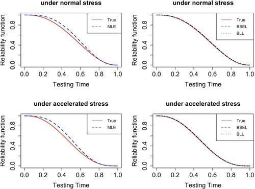
Figure 1 gives the values of all iterations obtained by the MCMC method and depicts the convergence of the method, where the white dashed line indicates the true values of the parameters. The histogram of all iteration points of the MCMC method is given in Figure 2, where the red curve represents the kernel density estimation function of the posterior density. These two graphs show that the MCMC method works very well. Also shown in Figure 3 are plots of the reliability functions obtained by different estimation methods under accelerated and normal stress.

8. A practical production example

This section uses the ALT real data set presented in Fu et al. (2009) to illustrate the feasibility of the model and statistical inference approach proposed in this paper. The real data set has also been studied in Wang et al. (2021) and Wang et al. (2022). This data set shows the failure data in constant stress ALT performed with temperature and vibration frequency as accelerated stresses for a specific type cylinder of ${\mathrm{CQ}}^2$ series product. It is mentioned in the Fu et al. (2009) that the cylinder consists of a series of grease, piston rubber ring, and piston rod, and then the cylinder system is 1-out-of-3:G system. In addition, the cylinder system has an operating temperature stress of ${35}^o\mathrm{C}$.

Figure 1. Sampling trace plot of parameters by MCMC method.

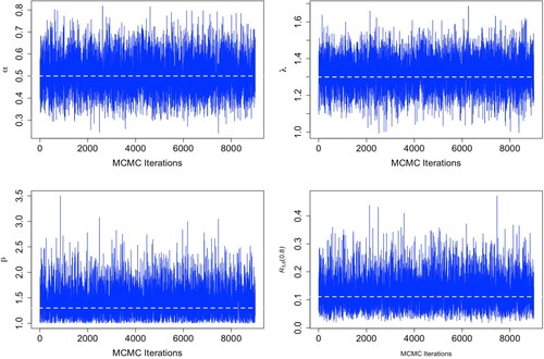
Figure 2. Histogram and kernel density estimates of parameters generated by the MCMC method.

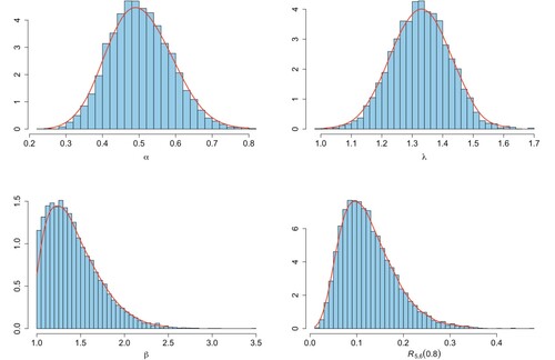
Figure 3. Comparison of the estimated reliability function with the true reliability function.

We analyse the constant stress PALT of the cylinder system and estimate the system reliability using temperature as the stress. Therefore, we fix the cylinder vibration frequency always at 50HZ, while we select the accelerated failure data at ${35}^o\mathrm{C}$, ${55}^o\mathrm{C}$ and ${75}^o\mathrm{C}$ and divide it into two groups, i.e., Group I (${35}^o\mathrm{C}$ and ${55}^o\mathrm{C}$) and Group II (${35}^o\mathrm{C}$ and ${75}^o\mathrm{C}$).

Considering the bounded property of the Kumaraswamy distribution, we divided all the data by $24\times {10}^6$. and the results are shown in the Table 11. We used the KS test to do a goodness-of-fit test on the distribution and the data. The values of the KS test statistic and the corresponding p-values are presented in Table 12, which shows that the Kumaraswamy distribution can be used as the underlying fitted distribution for the cylinder system reliability function.

Table 11. Failure times of the cylinder series system of ${\mathrm{CQ}}^2$ product.

Temperature	Failure times of three components	System lifetime
35${}^o\mathrm{C}$	0.750000 0.920833 0.979167	0.750000
	0.470833 0.470833 0.483333	0.470833
${55}^o\mathrm{C}$	0.406250 0.406250 0.425000	0.406250
	0.365417 0.389167 0.389583	0.365417
	0.067500 0.458333 0.466667	0.067500
${75}^o\mathrm{C}$	0.174167 0.195417 0.202917	0.174167
	0.202500 0.816667 0.816667	0.202500

Table 12. The KS tests under the different groups.

Group	Temperature	p-value	Value of KS statistic
I	${35}^o\mathrm{C}$	0.969400	0.252710
	${55}^o\mathrm{C}$	0.267600	0.275870
II	${35}^o\mathrm{C}$	0.621700	0.390250
	${75}^o\mathrm{C}$	0.114500	0.457270

The estimates of the correlation parameter for Kumaraswamy are presented in Tables 13 and 14. Its Bayesian estimates are obtained under non-informative prior conditions, i.e., $a_i=b_i=0.00001,i=1,2$. Furthermore, we set $\epsilon ={10}^{-16}$, $B=N=\mathrm{10,000}$, $\gamma =0.05$. Tables 13 and 14 show that the point estimates and interval estimates for α and λ are close. However, there is a minor discrepancy between the various estimates of the acceleration factor β.

In addition, although the non-informative prior leading to Bayesian estimation does not showing its full advantage, the numerical results show that the Bayesian method is still superior to the maximum likelihood estimation method in this example. The fitted CDFs and empirical distributions are compared in Figures 4 and  5.

Figure 4. Comparisons of empirical CDFs and the fitted Kumaraswamy CDFs under data group I.

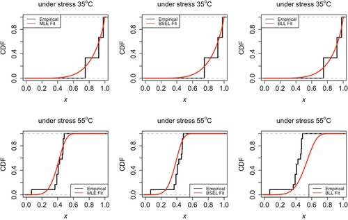
Figure 5. Comparisons of empirical CDFs and the fitted Kumaraswamy CDFs under data group II.

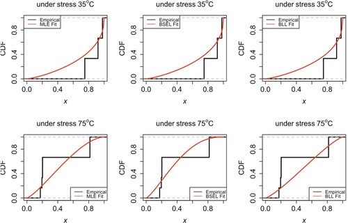
Table 13. Estimates for Kumaraswamy coefficient parameters under cylinder data group I.

	α	λ	β	$R_{1,3}(0.8)$
MLE	0.868486	5.292720	101.334900	$0.9808754$
BSEL	0.901132	5.295796	129.822000	0.967969
BLL	0.800744	5.293552	23.281220	0.966811
ACI	$(-0.112791,1.810159)$	$(4.825469,5.759971)$	$(-31.050930,233.720600)$	$(0.925418,1.036332)$
	[1.92295]	[0.934502]	[264.771530]	[0.110914]
BCI	$(0.229243,2.088398)$	$(5.183831,5.400598)$	$(33.426030,385.149600)$	$(0.850051,0.999468)$
	[1.859155]	[0.216767]	[351.723570]	[0.149417]
PBCI	$(0.365667,0.922738)$	$(3.815860,9.405010)$	$(20.249840,2734.810000)$	$(0.652495,0.999218)$
	[0.557071]	[5.58915]	[2714.560160]	[0.346723]

Table 14. Estimates for Kumaraswamy coefficient parameters under cylinder data group II.

	α	λ	β	$R_{1,3}(0.8)$
MLE	0.424785	1.300140	4.116810	0.912866
BSEL	0.417519	1.287583	5.719851	0.897099
BLL	0.393578	1.265287	3.028262	0.891172
ACI	$(-0.070523,0.920092)$	$(0.364078,2.236202)$	$(-1.744579,9.978199)$	$(0.692882,1.132850)$
	[0.990615]	[1.872124]	[11.722778]	[0.439968]
BCI	$(0.101935,0.966458)$	$(0.871584,1.693853)$	$(1.316909,18.907130)$	$(0.616779,0.997461)$
	[0.864523]	[0.822269]	[17.590221]	[0.380682]
PBCI	$(0.186424,0.922738)$	$(0.731934,4.363940)$	$(0.703576,34.997240)$	$(0.060212,0.994506)$
	[0.736314]	[3.632006]	[34.293664]	[0.934294]

9. Concluding remarks

In this paper, we study parameter estimation and reliability inference for s-out-of-k: G systems with Kumaraswamy component lifetime distributions based on a constant stress PALT. We obtained different point and interval estimates by classical maximum likelihood estimation, Bayesian, and Bootstrap methods. Extensive Monte Carlo simulations compare the performance of these methods, and the results are satisfactory. The Bayesian estimation method generally performs better in the presence of additional prior information. Moreover, we study a real data set illustrating the methods used in this paper.

Based on this paper's research methodology and results, multicomponent systems' reliability estimation and properties can continue to be investigated under step stress and progressive stress ALT in future work. Meanwhile, studying optimal Bayesian design plans for systems with components following the Kumaraswamy lifetime distribution under the control of experimental costs is an interesting issue. In addition, current studies on ALT for multicomponent systems are based on the independent case between components, while the dependent case of the components is also a very interesting topic, e.g., (Guo et al., 2024; Zhang, Yan, Wang, et al., 2022; Zhang, Yan, Zhang, et al., 2022; Zhang & Zhang, 2022) used copula theory to deal with the dependency between components, and (J. Zhang et al., 2024; Zhang et al., 2023) modelled statistical dependence with the help of stochastic arrangement increasing. Therefore, we are eager to derive the ALT framework for multicomponent systems with dependent components in the future.

Acknowledgments

The authors are very grateful for the insightful and constructive comments and suggestions from the Editor-in-Chief, an Associate Editor, and two anonymous reviewers, which have greatly improved the presentation of this manuscript.

Disclosure statement

No potential conflict of interest was reported by the author(s).

Additional information

Funding

This work is supported by the National Natural Science Foundation of China [grant number 12361060], Funds for Innovative Fundamental Research Group Project of Gansu Province [grant number 23JRRA684] and College Teachers Innovation Foundation Project of Gansu Provincial Education Department [grant number 2024A-002].

Appendices

Appendix 1. Proof of Theorem

A.1. Proof of Theorem 3.1

By taking the derivative of Equation (8(8) $\begin{array}{rl}l(\alpha ,\lambda ,\beta \mid \underset{\_}{x})& \propto \mathrm{knlog}\lambda +\mathrm{knlog}\alpha +k{n}_1\log \beta +(\alpha -1)\sum _{j=1}^{n_0}\sum _{u=1}^k\log (1-x_{0:j:u}^{\lambda })\\ & +(\lambda -1)\sum _{i=0}^1\sum _{j=1}^{n_i}\sum _{u=1}^k\log x_{i:j:u}+(\mathrm{\beta \alpha }-1)\sum _{j=1}^{n_1}\sum _{u=1}^k\log (1-x_{1:j:u}^{\lambda }).\end{array}$(8) ) to β and setting it to zero, then (9(9) $\hat{\beta }=-\frac{k{n}_1}{\alpha \sum _{j=1}^{n_1}\sum _{u=1}^k\log (1-x_{1:j:u}^{\lambda })}.$(9) ) can be obtained simply. Then, we will demonstrate that the log-likelihood function (8(8) $\begin{array}{rl}l(\alpha ,\lambda ,\beta \mid \underset{\_}{x})& \propto \mathrm{knlog}\lambda +\mathrm{knlog}\alpha +k{n}_1\log \beta +(\alpha -1)\sum _{j=1}^{n_0}\sum _{u=1}^k\log (1-x_{0:j:u}^{\lambda })\\ & +(\lambda -1)\sum _{i=0}^1\sum _{j=1}^{n_i}\sum _{u=1}^k\log x_{i:j:u}+(\mathrm{\beta \alpha }-1)\sum _{j=1}^{n_1}\sum _{u=1}^k\log (1-x_{1:j:u}^{\lambda }).\end{array}$(8) ) will reach its maximal value at $\hat{\beta }$.

Let $t=\frac{\beta }{\hat{\beta }}$, using $\log t\le t-1$, and then we can obtain $\log \beta \le -\frac{\mathrm{\alpha \beta }}{k{n}_1}\sum _{j=1}^{n_1}\sum _{u=1}^k\log (1-x_{1:j:u}^{\lambda })-1+\log \hat{\beta }.$Hence, the log-likelihood function (8(8) $\begin{array}{rl}l(\alpha ,\lambda ,\beta \mid \underset{\_}{x})& \propto \mathrm{knlog}\lambda +\mathrm{knlog}\alpha +k{n}_1\log \beta +(\alpha -1)\sum _{j=1}^{n_0}\sum _{u=1}^k\log (1-x_{0:j:u}^{\lambda })\\ & +(\lambda -1)\sum _{i=0}^1\sum _{j=1}^{n_i}\sum _{u=1}^k\log x_{i:j:u}+(\mathrm{\beta \alpha }-1)\sum _{j=1}^{n_1}\sum _{u=1}^k\log (1-x_{1:j:u}^{\lambda }).\end{array}$(8) ) can be written as $\begin{array}{rl}l(\alpha ,\lambda ,\beta \mid \underset{\_}{x})& \le \mathrm{knlog}\lambda +\mathrm{knlog}\alpha +k{n}_1\log \hat{\beta }+(\alpha -1)\sum _{j=1}^{n_0}\sum _{u=1}^k\log (1-x_{0:j:u}^{\lambda })\\ & +(\lambda -1)\sum _{i=0}^1\sum _{j=1}^{n_i}\sum _{u=1}^k\log x_{i:j:u}-\sum _{j=1}^{n_1}\sum _{u=1}^k\log (1-x_{1:j:u}^{\lambda })-k{n}_1.\end{array}$From (9(9) $\hat{\beta }=-\frac{k{n}_1}{\alpha \sum _{j=1}^{n_1}\sum _{u=1}^k\log (1-x_{1:j:u}^{\lambda })}.$(9) ), we get $k{n}_1=-\hat{\beta }\alpha \sum _{j=1}^{n_1}\sum _{u=1}^k\log (1-x_{1:j:u}^{\lambda })$ inserted into the above inequality. Then we have $\begin{array}{rl}l(\alpha ,\lambda ,\beta |\underset{\_}{x})& \le \mathrm{knlog}\lambda +\mathrm{knlog}\alpha +k{n}_1\log \hat{\beta }+(\alpha -1)\sum _{j=1}^{n_0}\sum _{u=1}^k\log (1-x_{0:j:u}^{\lambda })\\ & +(\lambda -1)\sum _{i=0}^1\sum _{j=1}^{n_i}\sum _{u=1}^k\log x_{i:j:u}+(\hat{\beta }\alpha -1)\sum _{j=1}^{n_1}\sum _{u=1}^k\log (1-x_{1:j:u}^{\lambda })\\ & =l(\alpha ,\lambda ,\hat{\beta }|\underset{\_}{x})\end{array}$The equation holds when $\beta =\hat{\beta }$, so the proof is complete.

A.2. Proof of Theorem 3.2

Replace β in (8(8) $\begin{array}{rl}l(\alpha ,\lambda ,\beta \mid \underset{\_}{x})& \propto \mathrm{knlog}\lambda +\mathrm{knlog}\alpha +k{n}_1\log \beta +(\alpha -1)\sum _{j=1}^{n_0}\sum _{u=1}^k\log (1-x_{0:j:u}^{\lambda })\\ & +(\lambda -1)\sum _{i=0}^1\sum _{j=1}^{n_i}\sum _{u=1}^k\log x_{i:j:u}+(\mathrm{\beta \alpha }-1)\sum _{j=1}^{n_1}\sum _{u=1}^k\log (1-x_{1:j:u}^{\lambda }).\end{array}$(8) ) with (9(9) $\hat{\beta }=-\frac{k{n}_1}{\alpha \sum _{j=1}^{n_1}\sum _{u=1}^k\log (1-x_{1:j:u}^{\lambda })}.$(9) ) and re-express it as $\begin{array}{rl}l(\alpha ,\lambda \mid \underset{\_}{x})& \propto \mathrm{knlog}\lambda +\mathrm{knlog}\alpha -k{n}_1\log [\alpha \sum _{j=1}^{n_1}\sum _{u=1}^k\log (1-{x^{\lambda }}_{1:j:u})]\\ & +(\alpha -1)\sum _{j=1}^{n_0}\sum _{u=1}^k\log (1-x_{0:j:u}^{\lambda })+(\lambda -1)\sum _{i=0}^1\sum _{j=1}^{n_i}\sum _{u=1}^k\log x_{i:j:u}\\ & -\sum _{j=1}^{n_1}\sum _{u=1}^k\log (1-x_{1:j:u}^{\lambda }).\end{array}$By taking the first-order partial derivative of $l(\alpha ,\lambda \mid \underset{\_}{x})$ to α and letting it be $H(\alpha )$, we can obtain $H(\alpha )=\frac{k{n}_0}{\alpha }+\sum _{j=1}^{n_0}\sum _{u=1}^k\log (1-x_{0:j:u}^{\lambda }).$For $H(\alpha )$, because $x_{0:j:u}\in (0,1)$, use $\log (1-x_{0:j:u}^{\lambda })\le -x_{0:j:u}^{\lambda }$ to easily get $\underset{\alpha \to +\mathrm{\infty }}{lim}H(\alpha )<0,\mathrm{and}\underset{\alpha \to 0^{+}}{lim}H(\alpha )>0.$These two limits implied that $\hat{\alpha }$ exists.

And then consider $\frac{{\mathrm{\partial }}^{2}l(\alpha ,\lambda ,\beta \mid \underset{\_}{x})}{\mathrm{\partial }{\alpha }^2}=\frac{-k{n}_0}{{\alpha }^2}<0,$which suggests that the (8(8) $\begin{array}{rl}l(\alpha ,\lambda ,\beta \mid \underset{\_}{x})& \propto \mathrm{knlog}\lambda +\mathrm{knlog}\alpha +k{n}_1\log \beta +(\alpha -1)\sum _{j=1}^{n_0}\sum _{u=1}^k\log (1-x_{0:j:u}^{\lambda })\\ & +(\lambda -1)\sum _{i=0}^1\sum _{j=1}^{n_i}\sum _{u=1}^k\log x_{i:j:u}+(\mathrm{\beta \alpha }-1)\sum _{j=1}^{n_1}\sum _{u=1}^k\log (1-x_{1:j:u}^{\lambda }).\end{array}$(8) ) given λ is concave. Therefore, combining the above two results, it is proved that equation $l(\alpha ,\lambda ,\beta \mid \underset{\_}{x})$ has a unique maximal value at $\hat{\alpha }$ given λ.

Appendix 2. The elements of the observed Fisher information matrix

$\begin{array}{rl}\frac{{\mathrm{\partial }}^{2}l(\alpha ,\lambda ,\beta )}{\mathrm{\partial }{\alpha }^2}& =-\frac{\mathrm{kn}}{{\alpha }^2},\\ \frac{{\mathrm{\partial }}^{2}l(\alpha ,\lambda ,\beta )}{\mathrm{\partial }\alpha \mathrm{\partial \beta }}& =\sum _{j=1}^{n_1}\sum _{u=1}^k\log (1-x_{1:j:u}^{\lambda }),\\ \frac{{\mathrm{\partial }}^{2}l(\alpha ,\lambda ,\beta )}{\mathrm{\partial }\alpha \mathrm{\partial \lambda }}& =-\sum _{j=1}^{n_0}\sum _{u=1}^k\frac{x_{0:j:u}^{\lambda }\log x_{0:j:u}}{1-x_{0:j:u}^{\lambda }}-\beta \sum _{j=1}^{n_1}\sum _{u=1}^k\frac{x_{1:j:u}^{\lambda }\log x_{1:j:u}}{1-x_{1:j:u}^{\lambda }},\\ \frac{{\mathrm{\partial }}^{2}l(\alpha ,\lambda ,\beta )}{\mathrm{\partial }\beta \mathrm{\partial \alpha }}& =\frac{{\mathrm{\partial }}^{2}l(\alpha ,\lambda ,\beta )}{\mathrm{\partial }\alpha \mathrm{\partial \beta }},\\ \frac{{\mathrm{\partial }}^{2}l(\alpha ,\lambda ,\beta )}{\mathrm{\partial }{\beta }^2}& =-\frac{k{n}_1}{{\beta }^2},\\ \frac{{\mathrm{\partial }}^{2}l(\alpha ,\lambda ,\beta )}{\mathrm{\partial }\beta \mathrm{\partial \lambda }}& =-\alpha \sum _{j=1}^{n_1}\sum _{u=1}^k\frac{x_{1:j:u}^{\lambda }\log x_{1:j:u}}{1-x_{1:j:u}^{\lambda }},\\ \frac{{\mathrm{\partial }}^{2}l(\alpha ,\lambda ,\beta )}{\mathrm{\partial }\lambda \mathrm{\partial \alpha }}& =\frac{{\mathrm{\partial }}^{2}l(\alpha ,\lambda ,\beta )}{\mathrm{\partial }\alpha \mathrm{\partial \lambda }},\\ \frac{{\mathrm{\partial }}^{2}l(\alpha ,\lambda ,\beta )}{\mathrm{\partial }\lambda \mathrm{\partial \beta }}& =\frac{{\mathrm{\partial }}^{2}l(\alpha ,\lambda ,\beta )}{\mathrm{\partial }\beta \mathrm{\partial \lambda }},\\ \frac{{\mathrm{\partial }}^{2}l(\alpha ,\lambda ,\beta )}{\mathrm{\partial }{\lambda }^2}& =-\frac{\mathrm{kn}}{{\lambda }^2}-(\alpha -1)\sum _{j=1}^{n_0}\sum _{u=1}^k\frac{x_{0:j:u}^{\lambda }(\log x_{0:j:u}{)}^2}{(1-x_{0:j:u}^{\lambda }{)}^2}-(\mathrm{\beta \alpha }-1)\sum _{j=1}^{n_1}\sum _{u=1}^k\frac{x_{1:j:u}^{\lambda }(\log x_{1:j:u}{)}^2}{(1-x_{1:j:u}^{\lambda }{)}^2}.\end{array}$

References

- Aban, I., Meerschaert, M., & Panorska, A. (2006). Parameter estimation for the truncated Pareto distribution. Journal of the American Statistical Association, 101(473), 270–277. https://doi.org/10.1198/016214505000000411
- Aljohani, H. M., & Alfar, N. M. (2020). Estimations with step-stress partially accelerated life tests for competing risks Burr XII lifetime model under type-II censored data. Alexandria Engineering Journal, 59(3), 1171–1180. https://doi.org/10.1016/j.aej.2020.01.022
- Asa, A., Mhe, A., Hma, B., & Ae, C. (2022). Estimations of accelerated Lomax lifetime distribution with a dependent competing risks model under type-I generalized hybrid censoring scheme. Alexandria Engineering Journal, 61(8), 6489–6499. https://doi.org/10.1016/j.aej.2021.12.006
- Barlow, R., & Proschan, F. (1975). Statistical theory of reliability and life testing: Probability models. Holt, Rinehart and Winston.
- Bhattacharyya, G. K., & Johnson, R. A. (1974). Estimation of reliability in multicomponent stress-strength model. Journal of the American Statistical Association, 69(348), 966–970. https://doi.org/10.1080/01621459.1974.10480238
- Cai, J., Shi, Y., & Liu, B. (2020). Bayesian analysis for dependent competing risks model with masked causes of failure in step-stress accelerated life test under progressive hybrid censoring. Communications in Statistics – Simulation and Computation, 49(9), 2302–2320. https://doi.org/10.1080/03610918.2018.1517212
- Dey, S., Wang, L., & Nassar, M. (2022). Inference on Nadarajah-Haghighi distribution with constant stress partially accelerated life tests under progressive type-II censoring. Journal of Applied Statistics, 49(11), 2891–2912. https://doi.org/10.1080/02664763.2021.1928014
- Efron, B. (1982). The Jackknife, the Bootstrap and other resampling plans. Society for industrial and applied mathematics.
- Fan, T. H., & Hsu, T. M. (2014). Constant stress accelerated life test on a multiple-component series system under Weibull lifetime distributions. Communications in Statistics-Theory and Methods, 43(11), 2370–2383. https://doi.org/10.1080/03610926.2013.809115
- Fu, Y., Han, G., Chen, J., & Ma, J. (2009). Research of accelerated life test of complex system based on pneumatic system (in Chinese version). Journal of Mechanical Strength, 31(4), 578–583.
- Genc, A. (2013). Estimation of P(X>Y) with Topp-Leone distribution. Journal of Statistical Computation and Simulation, 83(2), 326–339. https://doi.org/10.1080/00949655.2011.607821
- Gholizadeh, R. A., Shirazi, M. A., & Mosalmanza, S. (2011). Classical and Bayesian estimations on the Kumaraswamy distribution using grouped and un-grouped data under difference loss functions. Journal of Applied Sciences, 11(12), 2154–2162. https://doi.org/10.3923/jas.2011.2154.2162
- Ghosh, I., & Nadarajah, S. (2017). On the Bayesian inference of Kumaraswamy distributions based on censored samples. Communication in Statistics-Theory and Methods, 46(17), 8760–8777. https://doi.org/10.1080/03610926.2016.1193197
- Greene, W. H. (2000). Econometric analysis (4th ed.). Wiley.
- Guo, Z., Zhang, J., & Yan, R. (2020). The residual lifetime of surviving components of coherent system under periodical inspections. Mathematics, 8(12), 2227–7390. https://doi.org/10.3390/math8122181
- Guo, Z., Zhang, J., & Yan, R. (2022). On inactivity times of failed components of coherent system under double monitoring. Probability in the Engineering and Informational Sciences, 36(3), 923–940. https://doi.org/10.1017/S0269964821000152
- Guo, M., Zhang, J., Zhang, Y., & Zhao, P. (2024). Optimal redundancy allocations for series systems under hierarchical dependence structures. Quality and Reliability Engineering International, 40(4), 1540–1565. https://doi.org/10.1002/qre.3508
- Hua, R., & Gui, W. (2022). Inference for copula-based dependent competing risks model with step-stress accelerated life test under generalized progressive hybrid censoring. Computational Statistics, 37(5), 2399–2436. https://doi.org/10.1007/s00180-022-01203-w
- Ismail, A. A. (2014). Inference for a step-stress partially accelerated life test model with an adaptive type-II progressively hybrid censored data from Weibull distribution. Journal of Computational and Applied Mathematics, 260, 533–542. https://doi.org/10.1016/j.cam.2013.10.014
- Ismail, A. A. (2016). Statistical inference for a step-stress partially-accelerated life test model with an adaptive type-I progressively hybrid censored data from Weibull distribution. Statistical Papers, 57(2), 271–301. https://doi.org/10.1007/s00362-014-0639-x
- Kizilaslan, F., & Nadar, M. (2016). Estimation and prediction of the Kumaraswamy distribution based on record values and inter-record times. Journal of Statistical Computation & Simulation, 86(12), 2471–2493. https://doi.org/10.1080/00949655.2015.1119832
- Kohansal, A. (2019). On estimation of reliability in a multicomponent stress-strength model for a Kumaraswamy distribution based on progressively censored sample. Statistical Papers, 60(6), 2185–2224. https://doi.org/10.1007/s00362-017-0916-6
- Kumaraswamy, P. (1980). A generalized probability density function for double-bounded random processes. Journal of Hydrology, 46(1-2), 79–88. https://doi.org/10.1016/0022-1694(80)90036-0
- Liu, B., Shi, Y., Zhang, F., & Bai, X. (2017). Reliability nonparametric Bayesian estimation for the masked data of parallel systems in step-stress accelerated life tests. Journal of Computational & Applied Mathematics, 311, 375–386. https://doi.org/10.1016/j.cam.2016.07.029
- Lu, B., Zhang, J., & Yan, R. (2023). Optimal allocation of a coherent system with statistical dependent subsystems. Probability in the Engineering and Informational Sciences, 37(1), 29–48. https://doi.org/10.1017/S0269964821000437
- Nelson, W. (2008). Accelerated testing: Statistical models, test plans, and data analysis. Wiley.
- Rastogi, M. K., Saad, J., Farghal, A. A., & G. A. Elmougod (2022). Partially constant-stress accelerated life tests model for parameters estimation of Kumaraswamy distribution under adaptive type-II progressive censoring. Alexandria Engineering Journal, 61(7), 5133–5143. https://doi.org/10.1016/j.aej.2021.10.035
- Roy, S. (2018). Bayesian accelerated life test plans for series systems with Weibull component lifetimes. Applied Mathematical Modelling, 62, 383–403. https://doi.org/10.1016/j.apm.2018.06.007
- Samanta, D., Gupta, A., & Kundu, D. (2019). Analysis of Weibull step-stress model in presence of competing risk. IEEE Transactions on Reliability, 68(2), 420–438. https://doi.org/10.1109/TR.24
- Wang, L. (2017). Inference of constant-stress accelerated life test for a truncated distribution under progressive censoring. Applied Mathematical Modelling, 44, 743–757. https://doi.org/10.1016/j.apm.2017.02.011
- Wang, L., Dey, S., Tripathi, Y. M., & Wu, S. J. (2020). Reliability inference for a multicomponent stress-strength model based on Kumaraswamy distribution. Journal of Computational and Applied Mathematics, 376, Article 112823. https://doi.org/10.1016/j.cam.2020.112823
- Wang, L., Wu, S. J., Zhang, C., Dey, S., & Tripathi, Y. M. (2022). Analysis for constant-stress model on multicomponent system from generalized inverted exponential distribution with stress dependent parameters. Mathematics and Computers in Simulation, 193(C), 301–316. https://doi.org/10.1016/j.matcom.2021.10.017
- Wang, L., Zhang, C., Tripathi, Y. M., Dey, S., & Wu, S. (2021). Reliability analysis of Weibull multicomponent system with stress-dependent parameters from accelerated life data. Quality and Reliability Engineering International, 37(6), 2603–2621. https://doi.org/10.1002/qre.v37.6
- Xu, A., Fu, J., Tang, Y., & Guan, Q. (2015). Bayesian analysis of constant-stress accelerated life test for the Weibull distribution using noninformative priors. Applied Mathematical Modelling, 39(20), 6183–6195. https://doi.org/10.1016/j.apm.2015.01.066
- Xu, A., & Tang, Y. (2011). Objective Bayesian analysis of accelerated competing failure models under type-I censoring. Computational Statistics & Data Analysis, 55(10), 2830–2839. https://doi.org/10.1016/j.csda.2011.04.009
- Yan, R., & Niu, J. (2022). Stochastic comparisons of second-order statistics from dependent and heterogenous modified proportional hazard rate observations. Statistics, 57(2), 328–353. https://doi.org/10.1080/02331888.2023.2177999
- Yan, R., Wang, J., & Lu, B. (2021). Orderings of component level versus system level at active redundancies for coherent systems with dependent components. Probability in the Engineering and Informational Sciences, 36(4), 1275–1297. https://doi.org/10.1017/S0269964821000401
- Yan, R., Zhang, J., & Wang, J. (2022). Optimal allocation of relevations in coherent systems. Journal of Applied Probability, 58(4), 293–298.
- Zhang, J., Guo, Z., Niu, J., & Yan, R. (2024). Increasing convex order of capital allocation with dependent assets under threshold model. Statistical Theory and Related Fields, 1–12. https://doi.org/10.1080/24754269.2023.2301630
- Zhang, C., Shi, Y., & Wu, M. (2016). Statistical inference for competing risks model in step-stress partially accelerated life tests with progressively type-I hybrid censored Weibull life data. Journal of Computational & Applied Mathematics, 297, 65–74. https://doi.org/10.1016/j.cam.2015.11.002
- Zhang, T., & Xie, M. (2011). On the upper truncated Weibull distribution and its reliability implications. Reliability Engineering & System Safety, 96(1), 194–200. https://doi.org/10.1016/j.ress.2010.09.004
- Zhang, J., Yan, R., & Wang, J. (2022). Reliability optimization of parallel-series and series-parallel systems with statistically dependent components. Applied Mathematical Modelling, 102, 618–639. https://doi.org/10.1016/j.apm.2021.10.003
- Zhang, J., Yan, R., & Zhang, Y. (2022). Reliability analysis of fail-safe systems with heterogeneous and dependent components subject to random shocks. Proceedings of the Institution of Mechanical Engineers, Part O: Journal of Risk and Reliability, 237(6), 1073–1087.
- Zhang, J., Yan, R., & Zhang, Y. (2023). Stochastic comparisons of largest claim amount from heterogeneous and dependent insurance portfolios. Journal of Computational and Applied Mathematics, 431, Article 115265. https://doi.org/10.1016/j.cam.2023.115265
- Zhang, J., & Zhang, Y. (2022). A copula-based approach on optimal allocation of hot standbys in series systems. Naval Research Logistics (NRL), 69(6), 902–913. https://doi.org/10.1002/nav.v69.6
- Zhang, J., & Zhang, Y. (2023). Stochastic comparisons of relevation allocation policies in coherent systems. Test, 32(3), 865–907. https://doi.org/10.1007/s11749-023-00855-0
- Zuo, M. J. (2003). Optimal reliability modeling, principles and applications. Wiley.