Spatial-sign-based high-dimensional white noises test

Abstract

In this study, we explore the problem of hypothesis testing for white noise in high-dimensional settings, where the dimension of the random vector may exceed the sample sizes. We introduce a test procedure based on spatial-sign for high-dimensional white noise testing. This new spatial-sign-based test statistic is designed to emulate the test statistic proposed by Paindaveine and Verdebout [(2016). On high-dimensional sign tests. Bernoulli, 22(3), 1745–1769.], but under a more generalized scatter matrix assumption. We establish the asymptotic null distribution and provide the asymptotic relative efficiency of our test in comparison with the test proposed by Feng et al. [(2022). Testing for high-dimensional white noise. arXiv:2211.02964.] under certain specific alternative hypotheses. Simulation studies further validate the efficiency and robustness of our test, particularly for heavy-tailed distributions.

Keywords:

• High-dimensional data
• spatial-sign
• white noise test

1. Introduction

In this paper, we consider testing for white noise or serial correlation, which is a fundamental problem in statistical inference. For univariate time series, the famous Box-Pierce portmanteau test and its variations are very popular due to their convenience in practical application (Li, 2003; Lütkepohl, 2005). Many efforts have been devoted to extending those methods for testing multivariate time series, such as Hosking (1980) and Li and McLeod (1981). Recently, high-dimensional time series data frequently appear in many applications, including finance and econometrics, biological and environmental research, etc., where the dimensions of the time series is comparable or even larger than the observed length of the time series. In this case, the above traditional white noise tests can not directly apply for high-dimensional data.

Recently, there are two types of omnibus tests proposed to deal with high-dimensional white noise test. One is the max-type test. Chang et al. (2017) proposed a test statistic using the maximum absolute autocorrelation and cross-correlations of the component series. Tsay (2020) proposed a rank-based max-type test using the Spearman rank correlation. Chen et al. (2022) extended Tsay (2020)'s work to other types rank-based correlations, such as Kendall's tau correlation and Hoeffding's D statistic, etc. As known to all, the max-type tests perform well for the sparse alternatives where only a few auto-correlations are nonzero and large, but perform less powerful for the dense alternatives where there are many small nonzero auto-correlations. So researchers proposed sum-type tests for the high-dimensional white noise test. Li et al. (2019) proposed a test statistic by using the sum of the squared singular values of several lagged sample autocovariance matrices. Feng et al. (2022) proposed a new sum-type test statistic by excluding some terms from the test statistic proposed by Li et al. (2019) and showed that it has better size performance. However, the above two sum-type tests are both based on the independent component model, which only allows the underlying distribution of the time series to be light tailed. Unfortunately, the assumption of light-tailed distribution may be no appropriate for many applications, such as stock security returns. Thus, we need to construct a robust high-dimensional white noise test procedure for the heavy tailed distributions.

The classic spatial-sign-based procedures are very robust and efficient in traditional multivariate analysis. See Oja (2010) for an overview. Recently, many literatures show that the spatial-sign-based procedures also perform very well in high-dimensional settings. Wang et al. (2015), Feng and Sun (2016) and Feng et al. (2021) proposed some spatial-sign-based test procedures for the high-dimensional one sample locationproblem. Feng et al. (2016) and Huang et al. (2023) considered high-dimensional two sample location problem. Zou et al. (2014) and Feng and Liu (2017) also extended the spatial-sign-based method to the high-dimensional sphericity test. Some spatial-sign-based test procedures for high-dimensional alpha test in factor pricing model were proposed by Liu et al. (2023), Zhao et al. (2022) and Zhao (2023). In an important work, Paindaveine and Verdebout (2016) proposed a spatial-sign-based test for i id.ness against serial dependence. However, they assume that the random vectors have independent spherical directions, which is too limited in applications. In practice, there is always some correlations between the random vectors. So we propose a new spatial-sign-based test procedure for the high-dimensional white noise test in this article. Under the elliptical symmetric distribution assumption, we establish the asymptotical normality of the proposed test statistic under the null hypothesis and a special alternative hypothesis. We also show that the asymptotical relative efficiency of our method with respect to the test proposed by Feng et al. (2022) is equivalent to the corresponding asymptotical relative efficiency of spatial-sign-based method with respect to the least-square based procedures in high-dimensional settings (Feng & Sun, 2016; Liu et al., 2023; Wang et al., 2015; Zhao, 2023). Simulation studies also demonstrate the superiority of our method for heavy-tailed distributions.

This paper is organized as follows. In Section 2, we introduce our proposed spatial-sign-based test procedure for high-dimensional white noise test and establish the theoretical results. Simulation studies are showed in Section 3. An application involving real data are presented in Section 4. The conclusion and additional discussion are provided in Section 5. All technical details are collected in Section 6.

2. Test procedure

Let ${\mathit{\epsilon }}_1,\dots ,{\mathit{\epsilon }}_n$ be a p-dimensional weakly stationary time series with a mean of zero. We consider the following testing problem: (1) $H_0:\left\{{\epsilon }_t\right\}\text{is white noise v s }{H}_1:\left\{{\epsilon }_t\right\}\text{is not white noise},$(1) where the dimension of time series p is comparable to or even greater than the sample size n. In this context, we define a time series $\{{\epsilon }_t\}$ as white noise if the elements ${\epsilon }_t$ are all independent and identically distributed. This definition differs from those provided in Shekhar et al. (2003) and Cai and Kwan (2022). Under the null hypothesis, $E({\mathit{\epsilon }}_t{\mathit{\epsilon }}_{t+k}^{\mathrm{\top }})=\mathbf{0}$. So, Li et al. (2019) proposed the following test statistic: $G_H=\sum _{h=1}^H\text{tr}({\hat{\mathbf{S}}}_h^{\mathrm{\top }}{\hat{\mathbf{S}}}_h),{\hat{\mathbf{S}}}_h=\frac{1}{n}\sum _{t=h+1}^n{\mathit{\epsilon }}_t{\mathit{\epsilon }}_{t-h}^{\mathrm{\top }}.$They established the asymptotical normality of $G_H$ by random matrix theory. Feng et al. (2022) removed the diagonal elements ${\mathit{\epsilon }}_i^{\mathrm{\top }}{\mathit{\epsilon }}_i{\mathit{\epsilon }}_{i+h}^{\mathrm{\top }}{\mathit{\epsilon }}_{i+h}$ from the summation and proposed the following test statistic: $T_{\mathrm{FLM}}=\frac{1}{n(n-1)}\sum _{h=1}^H\underset{s\ne t}{\sum \sum }{\mathit{\epsilon }}_t^{\mathrm{\top }}{\mathit{\epsilon }}_s{\mathit{\epsilon }}_{t+h}^{\mathrm{\top }}{\mathit{\epsilon }}_{s+h}.$They also established the asymptotical normality of $T_{\mathrm{FLM}}$ by the martingale central limit theorem. Both the above two tests need the assumption of an independent component model, that is, ${\mathit{\epsilon }}_t={\mathbf{S}}^{1/2}{\mathbf{z}}_t$ and ${\mathbf{z}}_t=(z_{t1},\dots ,z_{\mathrm{tp}}{)}^{\mathrm{\top }}$ is a sequence of independent random vectors of dimensions p with independent components. However, a common drawback of the independent component model is their inability to handle many well-known heavy-tailed distributions, such as the multivariate student t and the mixture of multivariate normal distributions. Thus, we need to propose a robust and efficient test procedure for heavy-tailed distributions.

Under the assumption that ${\mathit{\epsilon }}_t$ have independent spherical directions, Paindaveine and Verdebout (2016) proposed a standardization test statistic (2) $T_{\mathrm{PV}}=\frac{\sqrt{2p^2}}{\sqrt{H}}\sum _{h=1}^H\frac{1}{n-h}\sum _{h+1\le s<t\le n}{\mathit{U}}_{s-h}^{\mathrm{\top }}{\mathit{U}}_{t-h}{\mathit{U}}_s^{\mathrm{\top }}{\mathit{U}}_t,$(2) where ${\mathit{U}}_t=U({\mathit{\epsilon }}_t)$ and $U(\mathit{x})=\frac{\mathit{x}}{||\mathit{x}||}I(\mathit{x}\ne 0)$. They showed that $T_{\mathrm{PV}}\stackrel{d}{\to }N(0,1)$ as $n,p\to \mathrm{\infty }$ under the null hypothesis. However, the assumption of independent spherical directions always does not hold in practice. In addition, they did not give the power function of $T_{\mathrm{PV}}$ under the alternative hypothesis. So we need to establish the theoretical results of the spatial-sign-based test statistic under more general scatter matrix assumption.

We consider the following test statistic: (3) $T_S=\sum _{h=1}^H\frac{1}{n-h}\sum _{h+1\le s<t\le n}{\mathit{U}}_{s-h}^{\mathrm{\top }}{\mathit{U}}_{t-h}{\mathit{U}}_s^{\mathrm{\top }}{\mathit{U}}_t,$(3) which is mimic to the test statistic (2(2) $T_{\mathrm{PV}}=\frac{\sqrt{2p^2}}{\sqrt{H}}\sum _{h=1}^H\frac{1}{n-h}\sum _{h+1\le s<t\le n}{\mathit{U}}_{s-h}^{\mathrm{\top }}{\mathit{U}}_{t-h}{\mathit{U}}_s^{\mathrm{\top }}{\mathit{U}}_t,$(2) ). Next, we will show that the asymptotic variance of $T_S$ under the null hypothesis is $\frac{H}{2}{\mathrm{tr}}^2({\mathbf{\Omega }}^2)$ and $\mathbf{\Omega }=E({\mathit{U}}_t{\mathit{U}}_t^{\mathrm{\top }})$, which is equal to $\frac{H}{2}{p}^2$ if ${\mathit{\epsilon }}_t$ have independent spherical directions.

We need the following conditions.

(C1)

(Error Distribution) The error vectors ${\mathit{\epsilon }}_1,\dots ,{\mathit{\epsilon }}_n$ are i.i.d. from the p-variate mean zero elliptical distribution with probability density function: $\text{det}(\mathbf{\Xi }{)}^{-1/2}g(\Vert {\mathbf{\Xi }}^{-1/2}\mathit{\epsilon }\Vert ),\mathit{\epsilon }\in {\mathbb{R}}^p,$where $\mathbf{\Xi }$ is a positive-definite scatter matrix.

(C2)

(Covariance Matrix) $\mathrm{tr}({\mathbf{\Sigma }}^4)=o({\mathrm{tr}}^2({\mathbf{\Sigma }}^2))$ and $\frac{{\mathrm{tr}}^4(\mathbf{\Sigma })}{{\mathrm{tr}}^2({\mathbf{\Sigma }}^2)}\exp \{-\frac{{\mathrm{tr}}^2(\mathbf{\Sigma })}{128N{\lambda }_{max}^2(\mathbf{\Sigma })}\}\to 0$, where $\mathbf{\Sigma }=\mathrm{Cov}({\mathit{e}}_t)\doteq ({\sigma }_{\mathrm{ij}}{)}_{1\le i,j\le N}$ and ${\lambda }_{max}(\mathbf{\Sigma })$ is the largest eigenvalue of $\mathbf{\Sigma }$.

Under the Condition (C1), ${\mathit{\epsilon }}_i$ can be decomposed as ${\mathbf{\Xi }}^{1/2}{R}_i{u}_i$ where $u_i$ is a random vector uniformly distributed on the unit sphere in ${\mathbb{R}}^p$ and $R_i$ is a nonnegative random variable independent of $u_i$. The covariance matrix can be written as $\mathbf{\Sigma }=p^{-1}E(R_i^2)\mathbf{\Xi }$. Condition (C2) is the same as the Conditions (C1) and (C2) in Wang et al. (2015). If the eigenvalues of $\mathbf{\Sigma }$ are all bounded, Condition (C2) will hold.

Theorem 2.1

Under Conditions (C1)-(C2), we have $T_S/{\sigma }_S\stackrel{d}{\to }N(0,1)$ where ${\sigma }_S^2=\frac{H}{2}{\mathrm{tr}}^2({\mathbf{\Omega }}^2)$.

Then, we estimate $\widehat{\mathrm{tr}({\mathbf{\Omega }}^2)}$ as follows: $\widehat{\mathrm{tr}({\mathbf{\Omega }}^2)}=\frac{2}{n(n-1)}\sum _{1\le s<t\le n}({\mathit{U}}_s^{\mathrm{\top }}{\mathit{U}}_t{)}^2.$By Proposition 1 of Zhao (2023), we have $\widehat{\mathrm{tr}({\mathbf{\Omega }}^2)}/\mathrm{tr}({\mathbf{\Omega }}^2)\stackrel{p}{\to }1$ under the null hypothesis as $n,p\to \mathrm{\infty }$. So by Theorem 2.1, we reject the null hypothesis if $T_S/{\hat{\sigma }}_S>z_{\alpha }$ where ${\hat{\sigma }}_S^2=\frac{H}{2}\widehat{{\mathrm{tr}}^2({\mathbf{\Omega }}^2)}$ and $z_{\alpha }$ is the upper α quantile of standard normal distribution.

Next, we consider the power function of our test procedure. Specially, we consider the following alternative hypothesis: (4) $H_1:{\mathit{\epsilon }}_t={\mathbf{A}}_0{r}_t{\mathit{u}}_t+{\mathbf{A}}_1{r}_{t-1}{\mathit{u}}_{t-1},$(4) where ${\mathit{u}}_t$ is a random vector uniformly distributed on the unit sphere in ${\mathbb{R}}^p$ and $r_t$ is a nonnegative random variable independent of ${\mathit{u}}_t$. Let ${\mathbf{\Sigma }}_0={\mathbf{A}}_0^{\mathrm{\top }}{\mathbf{A}}_0$, ${\mathbf{\Sigma }}_1={\mathbf{A}}_1^{\mathrm{\top }}{\mathbf{A}}_1$ and ${\mathbf{\Sigma }}_{01}={\mathbf{A}}_0^{\mathrm{\top }}{\mathbf{A}}_1$. We also assume the following condition for ${\mathbf{A}}_0$ and ${\mathbf{A}}_1$.

(C3)	The eigenvalues of ${\mathbf{\Sigma }}_0$ are all bounded and $\mathrm{tr}({\mathbf{\Sigma }}_1)=O(p/n)$, $\mathrm{tr}({\mathbf{\Sigma }}_1^2)=O(p/n)$, $\mathrm{tr}({\mathbf{\Sigma }}_0{\mathbf{\Sigma }}_1)=O(p/n)$.

Theorem 2.2

Under $H_1$ in (4(4) $H_1:{\mathit{\epsilon }}_t={\mathbf{A}}_0{r}_t{\mathit{u}}_t+{\mathbf{A}}_1{r}_{t-1}{\mathit{u}}_{t-1},$(4) ) with Condition (C3) holding, if $p/n\to \gamma \in (0,\mathrm{\infty })$, we have, for H = 1, $\frac{T_S-\frac{1}{2}{c}_1^2{\omega }^{4}n{p}^{-2}\mathrm{tr}({\mathbf{\Sigma }}_0{\mathbf{\Sigma }}_1)}{\sqrt{1/2}{p}^{-2}{\omega }^4\mathrm{tr}({\mathbf{\Sigma }}_0^2)}\stackrel{d}{\to }N(0,1),$where $c_1=E(r_t)E(r_t^{-1})$ and $\omega =p^{-1/2}{\mathrm{tr}}^{1/2}({\mathbf{\Sigma }}_0)$.

Note that under Condition (C3), we have $\mathrm{tr}({\mathbf{\Omega }}^2)=\frac{\mathrm{tr}({\mathbf{\Sigma }}_0^2)}{{\mathrm{tr}}^2({\mathbf{\Sigma }}_0)}(1+o(1))$ under the null hypothesis. So, by Theorem 2.2, the power function of $T_S$ is ${\beta }_S=\underset{n,p\to \mathrm{\infty }}{lim}\mathrm{\Phi }(-z_{\alpha }+\frac{c_1^{2}n\mathrm{tr}({\mathbf{\Sigma }}_0{\mathbf{\Sigma }}_1)}{\sqrt{2}\mathrm{tr}({\mathbf{\Sigma }}_0^2)}).$In addition, according to Theorem 5 in Feng et al. (2022), the power function of the sum-type test proposed by Feng et al. (2022) is ${\beta }_{\mathrm{FLM}}=\underset{n,p\to \mathrm{\infty }}{lim}\mathrm{\Phi }(-z_{\alpha }+\frac{n{E}^2(r_t)\mathrm{tr}({\mathbf{\Sigma }}_0{\mathbf{\Sigma }}_1)}{\sqrt{2}E(r_t^2)\mathrm{tr}({\mathbf{\Sigma }}_0^2)})$under Condition (C3). Thus, the asymptotic relative efficiency of our SS test with respect to FLM test is $\mathrm{ARE}(\mathrm{SS},\mathrm{FLM})=\underset{p\to \mathrm{\infty }}{lim}{E}^2(r_t^{-1})E(r_t^2)\ge \underset{p\to \mathrm{\infty }}{lim}\{E(r_t)E(r_t^{-1}){\}}^2\ge 1$by Cauchy inequality. Next, we consider three special distributions for ${\mathit{\epsilon }}_t$.

1. ${\mathit{\epsilon }}_t\sim N(\mathbf{0},{\mathbf{I}}_p)$. So, $r_{t}E(r_t^{-1})\stackrel{p}{\to }1$ and then $\mathrm{ARE}(\mathrm{SS},\mathrm{FLM})=1$.

2. ${\mathit{\epsilon }}_t\sim t_p(\mathbf{0},{\mathbf{I}}_p,v)$. So $E(r_t^{-1})=\frac{\mathrm{\Gamma }\{(v+1)/2\}}{v^{1/2}\mathrm{\Gamma }(v/2)}\frac{\mathrm{\Gamma }\{(p-1)/2\}}{\mathrm{\Gamma }(p/2)},E(r_t^2)=\frac{\mathrm{pv}}{v-2}$and then $\mathrm{ARE}(\mathrm{SS},\mathrm{FLM})=\frac{2}{v-2}{\left(\frac{\mathrm{\Gamma }((v+1)/2)}{\mathrm{\Gamma }(v/2)}\right)}^2>1.$For v = 3, this value is about 2.54; for v = 4, it is about 1.76; for $v=\mathrm{\infty }$ (multivariate normal distribution), it converges to one.

3. ${\mathit{\epsilon }}_t\sim (1-v)N(\mathbf{0},{\mathbf{I}}_p)+\mathrm{vN}(\mathbf{0},{\sigma }^2{\mathbf{I}}_p)$. So $E(r_t^{-1})=\frac{\{v+(1-v)/\sigma \}{\{v+(1-v){\sigma }^2\}}^{1/2}}{2^{1/2}}\frac{\mathrm{\Gamma }\{(p-1)/2\}}{\mathrm{\Gamma }(p/2)},E(r_t^2)=p(1-v+v{\sigma }^2)$and then $\mathrm{ARE}(\mathrm{SS},\mathrm{FLM})=\frac{1+v(1-v){(\sigma -{\sigma }^{-1})}^2}{1+v(1-v){(1-{\sigma }^{-1})}^2}>1.$

3. Simulations

We compare our method with the max-type test proposed by Chang et al. (2017) (abbreviated as MAX), the sum-type test (abbreviated as FLM) and the Fisher's combined probability test (abbreviated as FC) proposed by Feng et al. (2022). First, we consider the null hypothesis. To verify the robustness of the proposed testing method, we consider the following three scenarios for ${\mathit{\epsilon }}_t$:

1. Multivariate normal distribution. ${\mathit{\epsilon }}_t{\sim }^{\mathrm{iid}}N(\mathbf{0},\mathbf{\Sigma })$;

2. Multivariate t-distribution. ${\mathit{\epsilon }}_t{\sim }^{\mathrm{iid}}t(\mathbf{0},\mathbf{\Sigma },3)$;

3. Multivariate mixture normal distribution. ${\mathit{\epsilon }}_t$'s are independently generated from $\gamma f_p(\mathbf{0},\mathbf{\Sigma })+(1-\gamma )f_p(\mathbf{0},9\mathbf{\Sigma })$, denoted by ${\text{MN}}_{p,\gamma ,9}(\mathbf{0},\mathbf{\Sigma })$, where $f_p(\cdot ,\cdot )$ is the density function of p-variate multivariate normal distribution. γ is chosen to be 0.8.

Thereinto, $\mathbf{\Sigma }=({\sigma }_{\mathrm{ij}}{)}_{1\le i,j\le p}$, ${\sigma }_{\mathrm{ii}}=1$, $i=1,\dots ,p$, ${\sigma }_{\mathrm{ij}}=\frac{1}{2}(i-j{)}^{-2}$ with $i\ne j$. Table 1 reports the empirical sizes of SS, MAX, FLM, FC tests with n = 100, 200 and p = 40, 80, 100. From Table 1, we observe that both FLM and SS tests can control the empirical sizes in most cases. However, the empirical sizes of MAX test are a little conservative under the multivariate normal distribution, while a litter larger than the nominal level under the multivariate t-distribution. And the empirical sizes of FC tests also have the same performance as MAX test.

Table 1. Size performance of different tests.

		H = 1				H = 2				H = 3
n	p	MAX	SS	FLM	FC	MAX	SS	FLM	FC	MAX	SS	FLM	FC
		Multivariate normal distribution
100	40	0.011	0.053	0.055	0.042	0.005	0.051	0.052	0.028	0.008	0.042	0.044	0.023
100	80	0.008	0.035	0.041	0.022	0.008	0.038	0.039	0.019	0.007	0.059	0.058	0.03
100	120	0.003	0.049	0.049	0.029	0.008	0.057	0.059	0.029	0.006	0.053	0.052	0.017
200	40	0.015	0.069	0.061	0.046	0.017	0.062	0.058	0.048	0.017	0.037	0.044	0.037
200	80	0.014	0.054	0.051	0.038	0.018	0.053	0.059	0.031	0.012	0.05	0.05	0.038
200	120	0.01	0.05	0.051	0.035	0.011	0.054	0.05	0.031	0.012	0.044	0.039	0.016
		Multivariate t-distribution
100	40	0.068	0.053	0.049	0.079	0.082	0.059	0.052	0.079	0.097	0.065	0.044	0.104
100	80	0.067	0.049	0.047	0.074	0.11	0.047	0.054	0.118	0.115	0.039	0.044	0.116
100	120	0.088	0.04	0.045	0.091	0.11	0.045	0.036	0.113	0.132	0.045	0.036	0.129
200	40	0.075	0.06	0.046	0.095	0.097	0.058	0.056	0.115	0.126	0.061	0.046	0.133
200	80	0.1	0.049	0.04	0.107	0.14	0.048	0.029	0.131	0.177	0.061	0.037	0.173
200	120	0.113	0.05	0.053	0.11	0.162	0.047	0.048	0.166	0.22	0.06	0.05	0.207
		Mixture of multivariate normal distribution
100	40	0.035	0.057	0.058	0.072	0.047	0.068	0.05	0.056	0.029	0.043	0.052	0.051
100	80	0.047	0.046	0.048	0.075	0.039	0.041	0.038	0.051	0.043	0.036	0.037	0.045
100	120	0.04	0.046	0.045	0.058	0.046	0.048	0.041	0.057	0.033	0.05	0.053	0.049
200	40	0.031	0.054	0.055	0.068	0.031	0.052	0.047	0.052	0.025	0.059	0.045	0.049
200	80	0.044	0.053	0.061	0.064	0.045	0.052	0.063	0.073	0.038	0.051	0.036	0.066
200	120	0.035	0.054	0.049	0.058	0.049	0.049	0.048	0.067	0.045	0.034	0.039	0.064

Next, we compare the empirical power performance of the above four tests. We consider three models for ${\mathit{\epsilon }}_t$:

1. VAR(1) model: ${\mathit{\epsilon }}_t=\mathbf{A}{\mathit{\epsilon }}_{t-1}+{\mathbf{z}}_t$;

2. VMA(1) model: ${\mathit{\epsilon }}_t={\mathbf{z}}_t+\mathbf{A}{\mathbf{z}}_{t-1}$;

3. VARMA(1) model: ${\mathit{\epsilon }}_t=0.5\mathbf{A}{\mathit{\epsilon }}_{t-1}+{\mathbf{z}}_t+0.5\mathbf{A}{\mathbf{z}}_{t-1}$.

Here, ‘VAR(1)’, ‘VMA(1)’ and ‘VARMA(1)’ are the abbreviations of 1-order vector autoregressive process, vector moving average process and vector autoregressive moving average process, respectively. Here, ${\mathbf{z}}_t$ are generated from Scenarios (I)–(III) with $\mathbf{\Sigma }={\mathbf{I}}_p$. Let $\mathbf{A}=(a_{\mathrm{ij}}{)}_{1\le i,j\le p}$. We consider the alternative hypothesis with $a_{\mathrm{ij}}\ne 0,$ for $1\le i,j\le m$ and $a_{\mathrm{ij}}=0$ otherwise. Here, m controls the signal strength and sparsity of $\mathbf{A}$. We consider two cases for m : (1) dense case: $m=[0.8p]$ and $a_{\mathrm{ij}}\sim U(-\frac{1}{4\sqrt{m}},\frac{1}{4\sqrt{m}})$ for $1\le i,j\le m$; (2) sparse case: $m=[0.05p]$ and $a_{\mathrm{ij}}\sim U(-\frac{3}{4\sqrt{m}},\frac{3}{4\sqrt{m}})$ for $1\le i,j\le m$. Table 2 reports the empirical power of the above four tests with n = 200, p = 80. Under the multivariate normal distribution, the performance of SS test is similar to FLM test, which is consistent to the theoretical result. Under the dense case, the powers of sum-type tests–SS and FLM are more powerful than MAX and FC tests. However, MAX and FC tests outperform SS and FLM tests under the sparse case. For the heavy-tailed distributions, our SS test has better performance than FLM test, which shows the advantage of the spatial-sign-based method. In addition, we found that the powers of the SS and FLM tests with H = 1 are larger than those tests with H = 2, 3. It is not strange because we consider the alternative hypothesis with 1-order. How to choose the best H for the general case deserves some further studies.

Table 2. Power performance of different tests with n = 200, p = 80.

		H = 1				H = 2				H = 3
	Model	MAX	SS	FLM	FC	MAX	SS	FLM	FC	MAX	SS	FLM	FC
		Multivariate normal distribution
Dense	(i)	0.021	0.729	0.725	0.585	0.024	0.497	0.51	0.35	0.02	0.38	0.39	0.262
	(ii)	0.016	0.698	0.71	0.559	0.016	0.46	0.465	0.318	0.015	0.358	0.374	0.222
	(iii)	0.01	0.732	0.737	0.595	0.016	0.49	0.484	0.348	0.011	0.368	0.379	0.242
Sparse	(i)	0.733	0.613	0.625	0.852	0.701	0.528	0.534	0.802	0.658	0.417	0.423	0.742
	(ii)	0.464	0.371	0.374	0.603	0.383	0.234	0.24	0.482	0.326	0.185	0.191	0.411
	(iii)	0.603	0.476	0.488	0.738	0.524	0.303	0.32	0.622	0.467	0.254	0.261	0.563
		Multivariate t-distribution
Dense	(i)	0.193	0.952	0.718	0.673	0.188	0.809	0.482	0.487	0.204	0.637	0.39	0.44
	(ii)	0.195	0.939	0.709	0.669	0.192	0.745	0.445	0.456	0.213	0.588	0.366	0.427
	(iii)	0.174	0.939	0.736	0.674	0.197	0.758	0.497	0.477	0.238	0.629	0.379	0.449
Sparse	(i)	0.766	0.879	0.597	0.862	0.768	0.813	0.506	0.834	0.745	0.708	0.436	0.813
	(ii)	0.595	0.559	0.361	0.697	0.546	0.353	0.235	0.609	0.536	0.266	0.194	0.594
	(iii)	0.688	0.739	0.456	0.791	0.683	0.567	0.309	0.742	0.636	0.43	0.243	0.684
		Mixture of multivariate normal distribution
Dense	(i)	0.059	0.931	0.748	0.641	0.048	0.771	0.533	0.429	0.052	0.596	0.379	0.311
	(ii)	0.042	0.917	0.723	0.612	0.043	0.703	0.49	0.388	0.058	0.525	0.386	0.305
	(iii)	0.042	0.938	0.743	0.609	0.056	0.723	0.47	0.368	0.055	0.571	0.382	0.301
Sparse	(i)	0.75	0.846	0.597	0.86	0.736	0.771	0.513	0.807	0.697	0.667	0.444	0.778
	(ii)	0.486	0.515	0.363	0.635	0.438	0.341	0.245	0.531	0.399	0.267	0.195	0.472
	(iii)	0.635	0.711	0.488	0.778	0.585	0.544	0.323	0.669	0.523	0.413	0.255	0.605

4. Application

In this section, we are interested in testing whether the error series $\{{\mathit{\epsilon }}_t\}$ under Sharpe-Lintner Capital Asset Pricing Model (CAPM) (Lintner, 1975; Sharpe, 1964) is white noise, i.e. (5) $H_0:\{{\mathit{\epsilon }}_t\}\text{is white noise v.s.}{H}_1:\{{\mathit{\epsilon }}_t\}\text{is not white noise},$(5) where ${\mathit{\epsilon }}_t=({\epsilon }_{t1},\dots ,{\epsilon }_{\mathrm{tp}}{)}^{\mathrm{\top }}$ and p is the number of securities. The CAPM model is one of the most popular factor pricing models in finance, which has the explicit form $Y_{\mathrm{ti}}=r_{\mathrm{ti}}-r_{\mathrm{ft}}={\alpha }_i+{\beta }_{i1}(r_{\mathrm{mt}}-r_{\mathrm{ft}})+{\epsilon }_{\mathrm{ti}}$for $t\in \{1,\dots ,n\}$ and $i\in \{1,\dots ,p\}$, where $r_{\mathrm{ti}}$ is the return of the ith security at time t, $r_{\mathrm{ft}}$ is the risk free rate at time t, $Y_{\mathrm{ti}}=r_{\mathrm{ti}}-r_{\mathrm{ft}}$ is the excess return of the ith security at time t and $r_{\mathrm{mt}}$ is the market return at time t. We gathered return data for the securities listed in the S&P 500 index. Initially, we compiled the monthly returns of all the securities in the S&P 500 index from January 2005 to November 2018. As the composition of the index changes over time, we focused on p = 374 securities that remained in the S&P 500 index throughout the entire period. This resulted in a total of T = 165 consecutive observations. The time series data for the safe rate of return and the market factors were sourced from Ken French's data library web page. We selected the one-month US treasury bill rate as the risk-free rate ($r_{\mathrm{ft}}$). The value-weighted return on all NYSE, AMEX, and NASDAQ stocks from CRSP served as a proxy for the market return ($r_{\mathrm{mt}}$).

Specifically, we let ${\hat{\epsilon }}_{\mathrm{ti}}\doteq Y_{\mathrm{ti}}-{\hat{\alpha }}_i-{\hat{\beta }}_{i1}(r_{\mathrm{mt}}-r_{\mathrm{ft}}),$where ${\hat{\alpha }}_i$ and ${\hat{\beta }}_{i1}$ are the ordinary least-squares (OLS) estimators of ${\alpha }_i$ and ${\beta }_{i1}$, respectively. To demonstrate the usefulness of the proposed test, we treat ${\hat{\mathit{\epsilon }}}_t=({\hat{\epsilon }}_{t1},\dots ,{\hat{\epsilon }}_{\mathrm{tp}}{)}^{\mathrm{\top }}$ as the observation of ${\mathit{\epsilon }}_t$, instead of considering the testing problem within the CAPM model. First, we applied SS, FLM, MAX and CC tests for the total samples. All the tests reject the null hypothesis at significant level 0.05. We apply the Box-Pierce test, a conventional autocorrelation test, to the residuals of each security under the CAPM model with the total sample sizes. The histogram of p-values from the Box-Pierce test for the U.S. datasets is shown in Figure 1. We also observe some autocorrelations for some securities. So for the following application, we employ the sliding window method. With a predetermined length n, we carry out each of the necessary tests on the data gathered from the period spanning τ to $\tau +n-1$ for every τ in the range of $\{1,\dots ,T-n\}$. 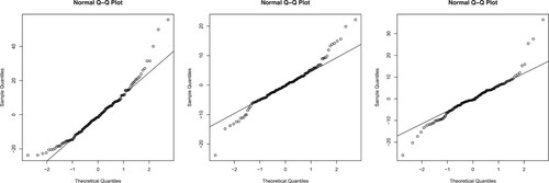Here, $\{\tau ,\dots ,\tau +n-1\}$ represents the sliding window of length n. Figure 2 displays the p-values for each test with a length of n = 36 (equivalent to three years). Our findings indicate that the MAX test is unable to reject the null hypothesis when the sample size is not sufficiently large. In most instances, the p-values of our proposed SS test are lower than those of the FLM test. Furthermore, we documented the frequency of null hypothesis rejection for the FLM and SS tests in these T−n test results, corresponding to the T−n sliding windows, which resulted in rates of 0.74 and 0.84, respectively. This indicates that our proposed SS test outperforms the other three tests in this application, primarily due to the heavy-tailed nature of the residuals. Figure 3 provides some Q-Q plots of these residuals.

Figure 1. Histogram of p-values of the Box-Pierce of residuals of CAPM model for U.S.'s datasets.

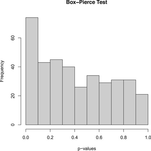
Figure 2. p-values of white noise tests for the U.S.'s datasets with CAPM model.

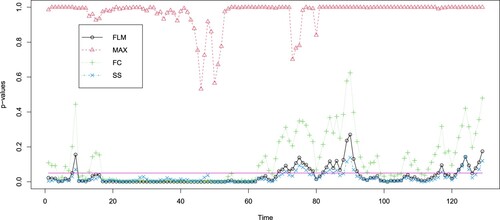
Figure 3. Q–Q plots of the residuals of three securities with CAPM model.

5. Conclusion

In this study, we develop a new test procedure for high-dimensional white noise testing based on spatial-sign. Unlike the method proposed by Feng et al. (2022), which constructs their test statistic using sample auto-covariance, our test statistic is constructed using auto-spatial-sign-covariance.We provide theoretical results for our proposed methods under the assumption of an elliptical distribution. Furthermore, we establish the asymptotic relative efficiency of our test in comparison to the sum-type test proposed by Feng et al. (2022). Our simulation studies and application to real data demonstrate the superiority of our method over the sum-type test proposed by Feng et al. (2022), particularly for heavy-tailed distributions.

As revealed in our simulation studies, our proposed test does not perform well against sparse alternatives. However, the max-type test proposed by Feng et al. (2022) can not control the empirical sizes under heavy tailed distributions. This makes it intriguing to develop a max-type test procedure based on spatial-sign for high-dimensional white noise testing. Moreover, Feng et al. (2022) demonstrated the asymptotic independence between their sum-type test statistic and the max-type test statistic. It would be interesting to investigate if the spatial-sign-based max-type test statistic also exhibits asymptotic independence with our proposed spatial-sign based sum-type test statistic. If this is the case, then we could construct a new combined test procedure based on this finding.

Disclosure statement

No potential conflict of interest was reported by the author(s).

Additional information

Funding

The research of Dachuan Chen is supported by the National Natural Science Foundation of China (Grants 12101335 and 12271271), the Natural Science Foundation of Tianjin (Grant 21JCQNJC00020), the Fundamental Research Funds for the Central Universities, Nankai University (Grants 63211088, 63221050, and 63231013) and Wukong Investment Research Funds. Zhao and Wang's research is partially supported by the China National Key R&D Program under Grant Nos. 2022YFA1003703, 2022YFA1003800, and 2019YFC1908502, the National Natural Science Foundation of China under Grant Nos. 12226007, 12271271, 11925106, 12231011, 11931001 and 11971247, the Fundamental Research Funds for the Central Universities under Grant No. ZB22000105 and Shenzhen Wukong Investment Management Co. Ltd..

Appendix

Proof of theorems

A.1. Proof of Theorem 2.1

Define $V_{\mathrm{nj}}=\sum _{l=1}^H\frac{1}{n-l}\sum _{i=l+1}^{j-1}{\mathit{U}}_{i-l}^{\mathrm{\top }}{\mathit{U}}_{j-l}{\mathit{U}}_i^{\mathrm{\top }}{\mathit{U}}_j,$for $j\in \{3,\dots ,n\}$ and $W_{\mathrm{nk}}=\sum _{i=3}^k{V}_{\mathrm{ni}}$, $k\in \{3,\dots ,n\}$. Let ${\mathcal{F}}_i\doteq \sigma \{{\mathit{U}}_1,\dots ,{\mathit{U}}_i\}$ be the σ-field generated by $\{{\mathit{U}}_j{\}}_{j\le i}$. It is easy to show that $E(V_{\mathrm{ni}}|{\mathcal{F}}_{i-1})=0$ and it follows that $\{W_{\mathrm{nk}},{\mathcal{F}}_k:3\le k\le n\}$ is a zero mean martingale. Let $v_{\mathrm{ni}}=E(V_{\mathrm{ni}}^2|{\mathcal{F}}_{i-1})$, $3\le i\le n$ and $V_n=\sum _{i=3}^n{v}_{\mathrm{ni}}$. The central limit theorem (Hall & Heyde, 1980) will hold if we can show (A1) $\frac{V_n}{\mathrm{Var}(W_{\mathrm{nn}})}\stackrel{p}{\to }1,$(A1) and for any $ϵ>0$, (A2) $\sum _{i=3}^n{\sigma }_S^{-2}E\left[V_{\mathrm{ni}}^2\mathbb{I}\{|V_{\mathrm{ni}}|>ϵ{\sigma }_S\}|{\mathcal{F}}_{i-1}\right]\stackrel{p}{\to }0.$(A2) It can be shown that $\begin{array}{rl}{v}_{\mathrm{ni}}& =\sum _{h,g=1}^H\frac{1}{(n-h)(n-g)}\sum _{s=h+1}^{i-1}\sum _{t=g+1}^{i-1}E({\mathit{U}}_{s-h}^{\mathrm{\top }}{\mathit{U}}_{i-h}{\mathit{U}}_s^{\mathrm{\top }}{\mathit{U}}_i{\mathit{U}}_{t-g}^{\mathrm{\top }}{\mathit{U}}_{i-g}{\mathit{U}}_t^{\mathrm{\top }}{\mathit{U}}_i\mid {\mathcal{F}}_{i-1})\\ & =\sum _{h=1}^H\frac{1}{(n-h{)}^2}\sum _{s=h+1}^{i-1}({\mathit{U}}_{s-h}^{\mathrm{\top }}{\mathit{U}}_{i-h}{)}^2{\mathit{U}}_s^{\mathrm{\top }}\mathbf{\Omega }{\mathit{U}}_s\\ & +\sum _{h=1}^H\frac{2}{(n-h{)}^2}\sum _{h+1\le s<t\le i-1}{\mathit{U}}_{s-h}^{\mathrm{\top }}{\mathit{U}}_{i-h}{\mathit{U}}_{t-h}^{\mathrm{\top }}{\mathit{U}}_{i-h}{\mathit{U}}_s^{\mathrm{\top }}\mathbf{\Omega }{\mathit{U}}_t.\end{array}$So $\begin{array}{rl}\frac{V_n}{\mathrm{Var}(W_{\mathrm{nn}})}& ={\sigma }_S^{-2}\sum _{i=3}^n\sum _{h=1}^H\frac{1}{(n-h{)}^2}\sum _{s=h+1}^{i-1}({\mathit{U}}_{s-h}^{\mathrm{\top }}{\mathit{U}}_{i-h}{)}^2{\mathit{U}}_s^{\mathrm{\top }}\mathbf{\Omega }{\mathit{U}}_s\\ & +{\sigma }_S^{-2}\sum _{i=3}^n\sum _{h=1}^H\frac{2}{(n-h{)}^2}\sum _{h+1\le s<t\le i-1}{\mathit{U}}_{s-h}^{\mathrm{\top }}{\mathit{U}}_{i-h}{\mathit{U}}_{t-h}^{\mathrm{\top }}{\mathit{U}}_{i-h}{\mathit{U}}_s^{\mathrm{\top }}\mathbf{\Omega }{\mathit{U}}_t\\ & \doteq C_{n1}+C_{n2}.\end{array}$Simple algebras lead to $E(C_{n1})=\frac{2}{H}\sum _{h=1}^H\frac{1}{(n-h{)}^2}\sum _{i=h+2}^n(i-h-1)=\frac{1}{H}\sum _{h=1}^H\frac{n-h-1}{n-h}\to 1$as $n\to \mathrm{\infty }$. And $\begin{array}{rl}\mathrm{Var}(C_{n1})& \le H{\sigma }_S^{-4}\sum _{h=1}^H\frac{1}{(n-h{)}^4}\mathrm{Var}[\sum _{i=3}^n\sum _{s=h+1}^{i-1}({\mathit{U}}_{s-h}^{\mathrm{\top }}{\mathit{U}}_{i-h}{)}^2{\mathit{U}}_s^{\mathrm{\top }}\mathbf{\Omega }{\mathit{U}}_s]\\ & \le \frac{H}{(n-H{)}^4{\sigma }_S^4}\sum _{h=1}^H\mathrm{Var}[\sum _{i=3}^n\sum _{s=h+1}^{i-1}({\mathit{U}}_{s-h}^{\mathrm{\top }}{\mathit{U}}_{i-h}{)}^2{\mathit{U}}_s^{\mathrm{\top }}\mathbf{\Omega }{\mathit{U}}_s]\\ & =O\left(n^{-1}\frac{E^2(({\mathit{U}}_t^{\mathrm{\top }}\mathbf{\Omega }{\mathit{U}}_t{)}^2)}{{\mathrm{tr}}^4({\mathbf{\Omega }}^2)}\right)\to 0\end{array}$by Lemma 1 in Wang et al. (2015). Thus, we have $C_{n1}\stackrel{p}{\to }1$. Similarly, $E(C_{n2})=0$ and $\mathrm{Var}(C_{n2})=O\left\{\frac{E^2\left\{{\left({\mathit{U}}_1^{\mathrm{\top }}\mathbf{\Omega }{\mathit{U}}_2\right)}^2\right\}+n^{-1}{E}^2\left\{{\left({\mathit{U}}_1^{\mathrm{\top }}\mathbf{\Omega }{\mathit{U}}_1\right)}^2\right\}}{{\mathrm{tr}}^4({\mathbf{\Omega }}^2)}\right\}\to 0.$So $C_{n2}\stackrel{p}{\to }0$. Consequently, (A1(A1) $\frac{V_n}{\mathrm{Var}(W_{\mathrm{nn}})}\stackrel{p}{\to }1,$(A1) ) holds.

To show (A2(A2) $\sum _{i=3}^n{\sigma }_S^{-2}E\left[V_{\mathrm{ni}}^2\mathbb{I}\{|V_{\mathrm{ni}}|>ϵ{\sigma }_S\}|{\mathcal{F}}_{i-1}\right]\stackrel{p}{\to }0.$(A2) ), we only need to prove that $\sum _{i=3}^{n}E(V_{\mathrm{ni}}^4)=o({\sigma }_S^4).$By Lemma 1 in Wang et al. (2015), we can show that $\sum _{i=3}^{n}E(V_{\mathrm{ni}}^4)=O(n^{-2}{E}^2({\mathit{U}}_1^{\mathrm{\top }}{\mathit{U}}_2{)}^4+n^{-1}{E}^2(({\mathit{U}}_1^{\mathrm{\top }}{\mathit{U}}_2{)}^2({\mathit{U}}_1^{\mathrm{\top }}{\mathit{U}}_3{)}^2))=o({\mathrm{tr}}^4({\mathbf{\Omega }}^2)).$Here we complete the proof.

A.2. Proof of Theorem 2

$\begin{array}{rl}U({\mathit{\epsilon }}_t)& =U({\mathbf{A}}_0{r}_t{\mathit{u}}_t+{\mathbf{A}}_1{r}_{t-1}{\mathit{u}}_{t-1})=\frac{{\mathbf{A}}_0{r}_t{\mathit{u}}_t+{\mathbf{A}}_1{r}_{t-1}{\mathit{u}}_{t-1}}{||{\mathbf{A}}_0{r}_t{\mathit{u}}_t+{\mathbf{A}}_1{r}_{t-1}{\mathit{u}}_{t-1}||}\\ & =\frac{{\mathbf{A}}_0{r}_t{\mathit{u}}_t+{\mathbf{A}}_1{r}_{t-1}{\mathit{u}}_{t-1}}{r_t{p}^{-1/2}{\mathrm{tr}}^{1/2}({\mathbf{\Sigma }}_0)}\frac{r_t{p}^{-1/2}{\mathrm{tr}}^{1/2}({\mathbf{\Sigma }}_0)}{||{\mathbf{A}}_0{r}_t{\mathit{u}}_t+{\mathbf{A}}_1{r}_{t-1}{\mathit{u}}_{t-1}||}\\ & =({\mathbf{A}}_0{p}^{-1/2}{\mathrm{tr}}^{1/2}({\mathbf{\Sigma }}_0){\mathit{u}}_t+{\mathbf{A}}_1{r}_{t-1}{r}_t^{-1}{p}^{-1/2}{\mathrm{tr}}^{1/2}({\mathbf{\Sigma }}_0){\mathit{u}}_{t-1})(1+{\gamma }_t{)}^{-1/2},\end{array}$where $\begin{array}{rl}{\gamma }_t& =\frac{||{\mathbf{A}}_0{r}_t{\mathit{u}}_t+{\mathbf{A}}_1{r}_{t-1}{\mathit{u}}_{t-1}|{|}^2}{r_t^2{p}^{-1}\mathrm{tr}({\mathbf{\Sigma }}_0)}-1\\ & =\frac{r_t^2{\mathit{u}}_t^{\mathrm{\top }}{\mathbf{\Sigma }}_0{\mathit{u}}_t+2r_t{r}_{t-1}{\mathit{u}}_t^{\mathrm{\top }}{\mathbf{\Sigma }}_{01}{\mathit{u}}_{t-1}+r_{t-1}^2{\mathit{u}}_{t-1}^{\mathrm{\top }}{\mathbf{\Sigma }}_1{\mathit{u}}_{t-1}}{r_t^2{p}^{-1}\mathrm{tr}({\mathbf{\Sigma }}_0)}-1\\ & =(\frac{{\mathit{u}}_t^{\mathrm{\top }}{\mathbf{\Sigma }}_0{\mathit{u}}_t}{p^{-1}\mathrm{tr}({\mathbf{\Sigma }}_0)}-1)+\frac{2r_{t-1}{\mathit{u}}_t^{\mathrm{\top }}{\mathbf{\Sigma }}_{01}{\mathit{u}}_{t-1}}{r_t{p}^{-1}\mathrm{tr}({\mathbf{\Sigma }}_0)}+\frac{r_{t-1}^2{\mathit{u}}_{t-1}^{\mathrm{\top }}{\mathbf{\Sigma }}_1{\mathit{u}}_{t-1}}{r_t^2{p}^{-1}\mathrm{tr}({\mathbf{\Sigma }}_0)}\\ & =G_1+G_2+G_3.\end{array}$By lemma 4 in Zou et al. (2014) and condition (C3), we have $E(G_1^2)=O(\mathrm{tr}({\mathbf{\Sigma }}_0^2)/p^2)=O(p^{-1}),E(G_2^2)=O(\mathrm{tr}({\mathbf{\Sigma }}_0{\mathbf{\Sigma }}_1)/p^2)=O(p^{-1}{n}^{-1})$ and $E(G_3^2)=O(p^{-2}({\mathrm{tr}}^2({\mathbf{\Sigma }}_1)+\mathrm{tr}({\mathbf{\Sigma }}_1^2)))=O(n^{-1}{p}^{-1}+n^{-2})$. So ${\gamma }_t=O_p(p^{-1/2})$. Thus, by taking the same procedure as the proof of Theorem 1 in Zhao et al. (2022), we have $\begin{array}{rl}{T}_S& =\frac{1}{n-1}\sum _{2\le s<t\le n}{\mathit{U}}_{s-1}^{\mathrm{\top }}{\mathit{U}}_{t-1}{\mathit{U}}_s^{\mathrm{\top }}{\mathit{U}}_t\\ & =\frac{1}{n-1}\sum _{2\le s<t\le n}({\mathbf{A}}_0{p}^{-1/2}{\mathrm{tr}}^{1/2}({\mathbf{\Sigma }}_0){\mathit{u}}_{s-1}+{\mathbf{A}}_1{r}_{s-2}{r}_{s-1}^{-1}{p}^{-1/2}{\mathrm{tr}}^{1/2}({\mathbf{\Sigma }}_0){\mathit{u}}_{s-2}{)}^{\mathrm{\top }}\\ & \times ({\mathbf{A}}_0{p}^{-1/2}{\mathrm{tr}}^{1/2}({\mathbf{\Sigma }}_0){\mathit{u}}_{t-1}+{\mathbf{A}}_1{r}_{t-2}{r}_{t-1}^{-1}{p}^{-1/2}{\mathrm{tr}}^{1/2}({\mathbf{\Sigma }}_0){\mathit{u}}_{t-2})\\ & \times ({\mathbf{A}}_0{p}^{-1/2}{\mathrm{tr}}^{1/2}({\mathbf{\Sigma }}_0){\mathit{u}}_s+{\mathbf{A}}_1{r}_{s-1}{r}_s^{-1}{p}^{-1/2}{\mathrm{tr}}^{1/2}({\mathbf{\Sigma }}_0){\mathit{u}}_{s-1}{)}^{\mathrm{\top }}\\ & \times ({\mathbf{A}}_0{p}^{-1/2}{\mathrm{tr}}^{1/2}({\mathbf{\Sigma }}_0){\mathit{u}}_t+{\mathbf{A}}_1{r}_{t-1}{r}_t^{-1}{p}^{-1/2}{\mathrm{tr}}^{1/2}({\mathbf{\Sigma }}_0){\mathit{u}}_{t-1})+o_p(p^{-1}).\end{array}$Let $\omega =p^{-1/2}{\mathrm{tr}}^{1/2}({\mathbf{\Sigma }}_0),{\delta }_t=r_{t-1}{r}_t^{-1}$. We can decompose $T_S$ as $\begin{array}{rl}{T}_S& =\frac{{\omega }^4}{n-1}\sum _{2\le s<t\le n}{\mathit{u}}_s^{\mathrm{\top }}{\mathbf{A}}_0^{\mathrm{\top }}{\mathbf{A}}_0{\mathit{u}}_t{\mathit{u}}_{t-1}^{\mathrm{\top }}{\mathbf{A}}_0^{\mathrm{\top }}{\mathbf{A}}_0{\mathit{u}}_{s-1}\\ & +\frac{{\omega }^4}{n-1}\sum _{2\le s<t\le n}{\delta }_{t-1}{\delta }_{s-1}{\mathit{u}}_{s-1}^{\mathrm{\top }}{\mathbf{A}}_1^{\mathrm{\top }}{\mathbf{A}}_1{\mathit{u}}_{t-1}{\mathit{u}}_{t-1}^{\mathrm{\top }}{\mathbf{A}}_0^{\mathrm{\top }}{\mathbf{A}}_0{\mathit{u}}_{s-1}\\ & +D_1+D_2+D_3+o_p(p^{-1}),\end{array}$where $\begin{array}{rl}{D}_1=& \frac{{\omega }^4}{n-1}\sum _{2\le s<t\le n}({\delta }_{s-1}{\delta }_{s-2}{\delta }_{t-1}{\delta }_{t-2}{\mathit{u}}_{s-1}^{\mathrm{\top }}{\mathbf{A}}_1^{\mathrm{\top }}{\mathbf{A}}_1{\mathit{u}}_{t-1}{\mathit{u}}_{t-2}^{\mathrm{\top }}{\mathbf{A}}_1^{\mathrm{\top }}{\mathbf{A}}_1{\mathit{u}}_{s-2}\\ & +{\delta }_{s-2}{\delta }_{t-2}{\mathit{u}}_s^{\mathrm{\top }}{\mathbf{A}}_0^{\mathrm{\top }}{\mathbf{A}}_0{\mathit{u}}_t{\mathit{u}}_{t-2}^{\mathrm{\top }}{\mathbf{A}}_1^{\mathrm{\top }}{\mathbf{A}}_1{\mathit{u}}_{s-2}),\\ D_2& =\frac{{\omega }^4}{n-1}\sum _{2\le s<t\le n}({\delta }_{t-1}{\mathit{u}}_s^{\mathrm{\top }}{\mathbf{A}}_0^{\mathrm{\top }}{\mathbf{A}}_1{\mathit{u}}_{t-1}{\mathit{u}}_{t-1}^{\mathrm{\top }}{\mathbf{A}}_0^{\mathrm{\top }}{\mathbf{A}}_0{\mathit{u}}_{s-1}+{\delta }_{s-1}{\mathit{u}}_{s-1}^{\mathrm{\top }}{\mathbf{A}}_1^{\mathrm{\top }}{\mathbf{A}}_0{\mathit{u}}_t{\mathit{u}}_{t-1}^{\mathrm{\top }}{\mathbf{A}}_0^{\mathrm{\top }}{\mathbf{A}}_0{\mathit{u}}_{s-1}\\ & +{\delta }_{s-1}{\delta }_{t-1}{\mathit{u}}_{s-1}^{\mathrm{\top }}{\mathbf{A}}_1^{\mathrm{\top }}{\mathbf{A}}_1{\mathit{u}}_{t-1}{\mathit{u}}_{t-1}^{\mathrm{\top }}{\mathbf{A}}_0^{\mathrm{\top }}{\mathbf{A}}_1{\mathit{u}}_{s-2}+{\delta }_{s-1}{\delta }_{t-1}{\delta }_{t-2}{\mathit{u}}_{s-1}^{\mathrm{\top }}{\mathbf{A}}_1^{\mathrm{\top }}{\mathbf{A}}_1{\mathit{u}}_{t-1}{\mathit{u}}_{t-2}^{\mathrm{\top }}{\mathbf{A}}_1^{\mathrm{\top }}{\mathbf{A}}_0{\mathit{u}}_{s-1}\\ & +{\delta }_{t-2}{\mathit{u}}_s^{\mathrm{\top }}{\mathbf{A}}_0^{\mathrm{\top }}{\mathbf{A}}_0{\mathit{u}}_t{\mathit{u}}_{t-2}^{\mathrm{\top }}{\mathbf{A}}_1^{\mathrm{\top }}{\mathbf{A}}_0{\mathit{u}}_{s-1}+{\delta }_{s-2}{\mathit{u}}_s^{\mathrm{\top }}{\mathbf{A}}_0^{\mathrm{\top }}{\mathbf{A}}_0{\mathit{u}}_t{\mathit{u}}_{t-1}^{\mathrm{\top }}{\mathbf{A}}_0^{\mathrm{\top }}{\mathbf{A}}_1{\mathit{u}}_{s-2}\\ & +{\delta }_{t-1}{\delta }_{t-2}{\delta }_{s-2}{\mathit{u}}_s^{\mathrm{\top }}{\mathbf{A}}_0^{\mathrm{\top }}{\mathbf{A}}_1{\mathit{u}}_{t-1}{\mathit{u}}_{t-2}^{\mathrm{\top }}{\mathbf{A}}_1^{\mathrm{\top }}{\mathbf{A}}_1{\mathit{u}}_{s-2}+{\delta }_{s-1}{\delta }_{t-2}{\delta }_{s-2}{\mathit{u}}_{s-1}^{\mathrm{\top }}{\mathbf{A}}_1^{\mathrm{\top }}{\mathbf{A}}_0{\mathit{u}}_t{\mathit{u}}_{t-2}^{\mathrm{\top }}{\mathbf{A}}_1^{\mathrm{\top }}{\mathbf{A}}_1{\mathit{u}}_{s-2}),\\ D_3& =\frac{{\omega }^4}{n-1}\sum _{2\le s<t\le n}({\delta }_{t-1}{\delta }_{s-2}{\mathit{u}}_s^{\mathrm{\top }}{\mathbf{A}}_0^{\mathrm{\top }}{\mathbf{A}}_1{\mathit{u}}_{t-1}{\mathit{u}}_{t-1}^{\mathrm{\top }}{\mathbf{A}}_0^{\mathrm{\top }}{\mathbf{A}}_1{\mathit{u}}_{s-2}+{\delta }_{s-1}{\delta }_{t-2}{\mathit{u}}_{s-1}^{\mathrm{\top }}{\mathbf{A}}_1^{\mathrm{\top }}{\mathbf{A}}_0{\mathit{u}}_t{\mathit{u}}_{t-2}^{\mathrm{\top }}{\mathbf{A}}_1^{\mathrm{\top }}{\mathbf{A}}_0{\mathit{u}}_{s-1}\\ & +{\delta }_{t-1}{\delta }_{t-2}{\mathit{u}}_s^{\mathrm{\top }}{\mathbf{A}}_0^{\mathrm{\top }}{\mathbf{A}}_1{\mathit{u}}_{t-1}{\mathit{u}}_{t-2}^{\mathrm{\top }}{\mathbf{A}}_1^{\mathrm{\top }}{\mathbf{A}}_0{\mathit{u}}_{s-1}+{\delta }_{s-1}{\delta }_{s-2}{\mathit{u}}_{s-1}^{\mathrm{\top }}{\mathbf{A}}_1^{\mathrm{\top }}{\mathbf{A}}_0{\mathit{u}}_t{\mathit{u}}_{t-1}^{\mathrm{\top }}{\mathbf{A}}_0^{\mathrm{\top }}{\mathbf{A}}_1{\mathit{u}}_{s-2}).\end{array}$After some tedious algebra, we have $E(D_1^2)=o(p^{-2}),E(D_2^2)=o(p^{-2}),E(D_3^2)=o(p^{-2})$by Condition (C3). Taking the same procedure as the proof of Theorem 2.1, we can show that $\frac{1}{(n-1)\sqrt{p^{-4}{\mathrm{tr}}^2({\mathbf{\Sigma }}_0^2)/2}}\sum _{2\le s<t\le n}{\mathit{u}}_s^{\mathrm{\top }}{\mathbf{A}}_0^{\mathrm{\top }}{\mathbf{A}}_0{\mathit{u}}_t{\mathit{u}}_{t-1}^{\mathrm{\top }}{\mathbf{A}}_0^{\mathrm{\top }}{\mathbf{A}}_0{\mathit{u}}_{s-1}\stackrel{d}{\to }N(0,1).$And $\begin{array}{rl}E\left(\frac{{\omega }^4}{n-1}\sum _{2\le s<t\le n}{\delta }_{t-1}{\delta }_{s-1}{\mathit{u}}_{s-1}^{\mathrm{\top }}{\mathbf{A}}_1^{\mathrm{\top }}{\mathbf{A}}_1{\mathit{u}}_{t-1}{\mathit{u}}_{t-1}^{\mathrm{\top }}{\mathbf{A}}_0^{\mathrm{\top }}{\mathbf{A}}_0{\mathit{u}}_{s-1}\right)& =\frac{1}{2}{c}_1^2{\omega }^{4}n{p}^{-2}\mathrm{tr}({\mathbf{\Sigma }}_0{\mathbf{\Sigma }}_1),\\ \mathrm{Var}\left(\frac{{\omega }^4}{n-1}\sum _{2\le s<t\le n}{\delta }_{t-1}{\delta }_{s-1}{\mathit{u}}_{s-1}^{\mathrm{\top }}{\mathbf{A}}_1^{\mathrm{\top }}{\mathbf{A}}_1{\mathit{u}}_{t-1}{\mathit{u}}_{t-1}^{\mathrm{\top }}{\mathbf{A}}_0^{\mathrm{\top }}{\mathbf{A}}_0{\mathit{u}}_{s-1}\right)& =c_1^2{\omega }^{4}n{p}^{-2}\mathrm{tr}({\mathbf{\Sigma }}_0{\mathbf{\Sigma }}_1)=o(p^{-2}).\end{array}$Thus, we have $\frac{T_S-\frac{1}{2}{c}_1^2{\omega }^{4}n{p}^{-2}\mathrm{tr}({\mathbf{\Sigma }}_0{\mathbf{\Sigma }}_1)}{\sqrt{1/2}{p}^{-2}{\omega }^4\mathrm{tr}({\mathbf{\Sigma }}_0^2)}\stackrel{d}{\to }N(0,1).$

References

- Cai, J., & Kwan, M. P. (2022). Detecting spatial flow outliers in the presence of spatial autocorrelation. Computers, Environment and Urban Systems, 96, 101833. https://doi.org/10.1016/j.compenvurbsys.2022.101833
- Chang, J., Yao, Q., & Zhou, W. (2017). Testing for high-dimensional white noise using maximum cross-correlations. Biometrika, 104(1), 111–127. https://doi.org/10.1093/biomet/asw066
- Chen, D., Song, F., & Feng, L. (2022). Rank based tests for high dimensional white noise. arXiv:2204.08402.
- Feng, L., & Liu, B. (2017). High-dimensional rank tests for sphericity. Journal of Multivariate Analysis, 155, 217–233. https://doi.org/10.1016/j.jmva.2017.01.003
- Feng, L., Liu, B., & Ma, Y. (2021). An inverse norm sign test of location parameter for high-dimensional data. Journal of Business & Economic Statistics, 39(3), 807–815. https://doi.org/10.1080/07350015.2020.1736084
- Feng, L., Liu, B., & Ma, Y. (2022). Testing for high-dimensional white noise. arXiv:2211.02964.
- Feng, L., & Sun, F. (2016). Spatial-sign based high-dimensional location test. Electronic Journal of Statistics, 10(2), 2420–2434. https://doi.org/10.1214/16-EJS1176
- Feng, L., Zou, C., & Wang, Z. (2016). Multivariate-sign-based high-dimensional tests for the two-sample location problem. Journal of the American Statistical Association, 111(514), 721–735. https://doi.org/10.1080/01621459.2015.1035380
- Hall, P., & Heyde, C. C. (1980). Martingale limit theory and its application. Academic Press.
- Hosking, J. R. (1980). The multivariate portmanteau statistic. Journal of the American Statistical Association, 75(371), 602–608. https://doi.org/10.1080/01621459.1980.10477520
- Huang, X., Liu, B., Zhou, Q., & Feng, L. (2023). A high-dimensional inverse norm sign test for two-sample location problems. Canadian Journal of Statistics, 51(4), 1004–1033. https://doi.org/10.1002/cjs.v51.4
- Li, W. K. (2003). Diagnostic checks in time series. Chapman and Hall/CRC.
- Li, Z., Lam, C., Yao, J., & Yao, Q. (2019). On testing for high-dimensional white noise. The Annals of Statistics, 47(6), 3382–3412. https://doi.org/10.1214/18-AOS1782
- Li, W. K., & McLeod, A. I. (1981). Distribution of the residual autocorrelations in multivariate ARMA time series models. Journal of the Royal Statistical Society Series B: Statistical Methodology, 43(2), 231–239. https://doi.org/10.1111/j.2517-6161.1981.tb01175.x
- Lintner, J. (1975). The valuation of risk assets and the selection of risky investments in stock portfolios and capital budgets. In Stochastic optimization models in finance (pp. 131–155). Elsevier.
- Liu, B., Feng, L., & Ma, Y. (2023). High-dimensional alpha test of linear factor pricing models with heavy-tailed distributions. Statistica Sinica, 33, 1389–1410.
- Lütkepohl, H. (2005). New introduction to multiple time series analysis. Springer.
- Oja, H. (2010). Multivariate nonparametric methods with R: An approach based on spatial signs and ranks. Springer Science & Business Media.
- Paindaveine, D., & Verdebout, T. (2016). On high-dimensional sign tests. Bernoulli, 22(3), 1745–1769. https://doi.org/10.3150/15-BEJ710
- Sharpe, W. F. (1964). Capital asset prices: A theory of market equilibrium under conditions of risk. The Journal of Finance, 19(3), 425–442.
- Shekhar, S., C. T. Lu, & Zhang, P. (2003). A unified approach to detecting spatial outliers. GeoInformatica, 7(2), 139–166. https://doi.org/10.1023/A:1023455925009
- Tsay, R. S. (2020). Testing serial correlations in high-dimensional time series via extreme value theory. Journal of Econometrics, 216(1), 106–117. https://doi.org/10.1016/j.jeconom.2020.01.008
- Wang, L., Peng, B., & Li, R. (2015). A high-dimensional nonparametric multivariate test for mean vector. Journal of the American Statistical Association, 110(512), 1658–1669. https://doi.org/10.1080/01621459.2014.988215
- Zhao, P. (2023). Robust high-dimensional alpha test for conditional time-varying factor models. Statistics, 57(2), 444–457. https://doi.org/10.1080/02331888.2023.2180003
- Zhao, P., Chen, D., & Zi, X. (2022). High-dimensional non-parametric tests for linear asset pricing models. Stat, 11(1), e490. https://doi.org/10.1002/sta4.v11.1
- Zou, C., Peng, L., Feng, L., & Wang, Z. (2014). Multivariate sign-based high-dimensional tests for sphericity. Biometrika, 101(1), 229–236. https://doi.org/10.1093/biomet/ast040