Forecasting natural gas consumption in residential and commercial sectors in the US

ABSTRACT

The paper proposes a parallel forecasting approach for weekly natural gas consumption in the US residential and commercial sectors, which models scrape data and ratio data separately and then combines the outputs to generate the forecasts. To improve forecasting accuracy, both semi-parametric and nonparametric models, including dynamic linear regression model and dynamic semi-parametric model, are adopted to model the effects of weather variables, and time series techniques are employed to address the serial correlation exhibited by the data. An algorithm focusing on forecasting accuracy is proposed to select the smoothing parameter for serially correlated data. The proposed model is empirically tested using data in the New England area from 2013 to 2018 and benchmarked against some deep learning approaches including Deep Neural Network, Long Short-Term Memory Neural Network, and Gated Recurrent Unit Neural Network methods. Overall, the results show that the proposed approach performs well in generating accurate forecasts.

KEYWORDS:

• Energy forecasting
• penalised regression
• smoothing parameter selection
• splines
• time series

1. Introduction

Natural gas represents a more efficient and cleaner fuel relative to other fossil options such as coal and petroleum and has an important role in supporting integration with renewable energy sources (Mac Kinnon et al., 2018; Sabo et al., 2011; Xu & Wang, 2010). According to the US Census Bureau’s 2012 American Community Survey, natural gas is the primary space heating fuel in Northeast, Midwest, and West, and almost half of US households use natural gas as their primary heating fuel. In the last decade, there is an increasing trend of natural gas usage in the US, which is also expected to continue in the next decades (Mac Kinnon et al., 2018). Forecasting of natural gas consumption is important to provide the stability of supply and distribution systems (Potočnik et al., 2014).

Natural gas consumption is predicted for different time horizons, ranging from long-term, medium-term, to short-term predictions (Soldo, 2012; Tamba et al., 2018). Generally, the long-term forecasting studies make annual projections of natural gas supply, demand, and consumption at the world- or national scales to provide decision support for governmental energy policy and infrastructure development (e.g., Gutierrez et al., 2005; Huntington, 2007; Karadede et al., 2017; Logan et al., 2013; Olgun et al., 2012; Ozdemir et al., 2016; Reynolds & Kolodziej, 2009; Valero & Valero, 2010; Wadud et al., 2011; Wang et al., 2013; Xu & Wang, 2010). Also, researchers have performed the medium-term projections to identify quarterly or monthly consumption of natural gas (e.g., Aras & Aras, 2004; Herbert, 1987; Herbert et al., 1987; Sailor & Munoz, 1997; Suykens et al., 1996). To predict natural gas consumption, the long- and medium-term forecasting models typically use social and economic data as inputs, such as GDP, income, population change, natural gas and other energy prices, energy reserves, productions, and consumptions data, which are less time sensitive. On the other hand, the short-term prediction of natural gas consumption focuses on high-resolution forecasting such as weekly, daily, and hourly predictions (Tamba et al., 2018), which are conducted mostly at the scales of regions (e.g., Panella et al., 2012), cities (e.g., Szoplik, 2015; Viet & Mandziuk, 2005), or distribution systems (e.g., Brown & Matin, 1995; Gelo, 2006; Piggott, 1983; Potočnik et al., 2014). In general, the short-term forecasting lies in a more dynamic setting and has high demand for accuracy.

In this study, we focus on short-term forecast of natural gas assumption in the US residential and commercial sectors. Accurate short-term forecasting is of significant economic and societal impacts for energy companies as well as consumers (Kizilaslan & Karlik, 2008). Energy companies are responsible for natural gas supply and distribution in a region. It is critical for them to have efficient forecasting models to accurately predict natural gas consumption in a timely manner to manage natural gas demand and supply. On the one hand, if the actual demand reaches over the forecast, the energy companies, especially local distribution companies, are forced to extract gas from storage, interrupt service to customers, or purchase additional gas on a spot market, but on the other hand, when the consumption is less than the forecast, those companies need to find a way to store the extra gas, spend more time to sell it, or leave it in the pipe and face the penalties imposed by the pipeline companies, which all result in higher operational costs (Pang, 2012). In the US, the agency of Energy Information Administration (EIA) is a reliable data source that provides monthly natural gas usage data for each state, which are believed to accurately represent the natural gas consumption. However, the releasing date of such data lags by 3 months, and the monthly aggregation tends to mitigate the weather sensitivity and smooth out the fluctuations in daily or weekly natural gas consumptions (please refer to the discussion of low-pass filter, Fan & Yao, 2003). Yet, day-to-day operations of natural gas supply and distribution are largely based on weekly schedules, especially for purchasing and storing. Thus, in order to effectively plan and manage their daily operations, the energy companies need to acquire accurate forecast with the forecasting horizon of several days (Potočnik & Govekar, 2010), especially considering the weather-induced volatility in the natural gas market. It is of great interest to develop forecasting models to predict natural gas consumption on a continuous week-to-week basis, which can help firms save purchasing costs as well as increase efficiency in dispatch scheduling and maintenance planning (Laib et al., 2018; Sabo et al., 2011). In the extant literature on short-term natural gas consumption forecasting, there are a number of forecasting models in daily and hourly terms, but very few studies have considered weekly consumption forecast. When the temporal scale or granularity for a forecasting problem changes, different methods need to be considered. Moreover, while research on forecasting natural gas consumption is of universal interests to all the countries, forecasting methods that are suitable for energy companies can be different because the natural gas market and regulation policy vary from country to country (Potočnik & Govekar, 2010). Currently, there lacks updated research on forecasting short-term natural gas consumption based on the US context. Therefore, to fill the gap, in this study, we specifically address the weekly natural gas consumption forecasting in the US.

It is widely recognised that the short-term natural gas consumption is subject to the strain of surging demand induced by severe weather conditions. Particularly in the US, since the deregulation in the mid-1980s, the natural gas market became highly sensitive to temperature-related demand because with no federal-regulated natural gas prices in place, abnormal weather condition and associated surge of demand for natural gas can produce significant natural gas pricing volatility (Timmer & Lamb, 2007). For example, between December 24, 2017, and January 3, 2018, due to surging consumption caused by record cold temperatures in 48 states, 9^°F lower than the 30-year (1981–2010) daily average for the same period, the natural gas prices for immediate delivery at key regional trading hubs rose dramatically. In contrast to the monthly average price of around $\mathrm{\$}3.4$ per million British thermal units (BTUs) in December for the previous 10 years, a new record price of immediate delivery was set on December 29, 2017, reaching $\mathrm{\$}64.49$ per million BTUs at the Northern Natural Ventura trading hub in Hancock County, Iowa. Accordingly, in the literature, the short-term forecasting models rely heavily on weather data, such as temperature, wind speed, or heating degree days, to capture the significant impact of weather on natural gas consumption (e.g., Brown & Matin, 1995; Piggott, 1983; Potočnik et al., 2014; Viet & Mandziuk, 2005). As found out by Sabo et al. (2011) in their study of comparing three mathematical models that use inputs such as hourly temperature and past consumption data in the city of Osijek (Croatia), the models in which natural gas consumption and temperature are related explicitly could provide most acceptable forecast. Following the same line, in this study, we build our forecasting model of weekly natural gas consumption by looking at weather-related parameters as primary explanatory variables, in addition to historical consumption data.

In the existing literature, various forecasting approaches have been applied to predict short-term natural gas consumption, including mathematical models (e.g., Sabo et al., 2011); statistical methods such as time series model (e.g., Panella et al., 2012), autoregressive integrated moving average (ARIMA; e.g., Ediger & Akar, 2007), or support vector regression (e.g., H. Liu et al., 2004; Zhu et al., 2015); artificial neural network (ANN) methods (e.g., Kaynar et al., 2011; Kizilaslan & Karlik, 2008); fuzzy logic methods (e.g., Azadeh et al., 2010; Kizilaslan & Karlik, 2008; Viet & Mandziuk, 2005); or combination of multiple approaches (Soldo et al., 2014). With many different forecasting methods being proposed for short-term natural gas consumption, researchers have made efforts to compare their performances. For example, Viet and Mandziuk (2005) examined several forecasting approaches including naive prediction, prediction using linear and quadratic regression models, prediction using a single feedforward network, prediction based on working days, combination of feedforward neural networks, temperature context networks, and prediction with a single fuzzy neural network. They tested those approaches using daily consumption, daily average temperature, and calendar data (working days or weekends) from two different regions in Poland on daily, weekly, and four weekly basis. Their results show that the temperature context networks in daily and weekly predictions and the combination of three neural modules in four-week prediction outperform the single neural and the single fuzzy neural approaches. On the other hand, in an attempt to identify the suitable forecasting tool in real-world short-term natural gas consumption, Potočnik et al. (2014) conducted a comparative study on methods such as linear models, neural network models, and support vector regression models in both their static and adaptive versions for daily natural gas consumption forecasting. They found that, in general, the adaptive models had improved forecasting performance over the static model for the local distribution company. It should be noted that the results of different studies might be affected by the data sets used in those studies. As pointed out by Chen et al. (2016), different methods have their own merits and limitations. More interestingly, Viet and Mandziuk (2005) suggested that in their experiments, because the linear and quadratic regression models appeared to be visibly worse than neural-based methods, the prediction of natural gas consumption is most probably highly nonlinear. However, Potočnik et al. (2014) revealed that nonlinear models do not outperform linear models in terms of generalisation performance. Therefore, in this study, we consider nonparametric methods to allow the data to speak for themselves, linear or nonlinear.

For the purpose of this study, we seek to propose an effective method that is practically executable for energy companies and can deliver accurate results. When making short-term forecasts, energy companies are faced with one challenge, that is, they need timely access to input data but only have limited access to exterior data sources, which affects the timeliness and accuracy of their forecast results and the subsequent decision making. Therefore, in this study, we develop a forecasting strategy with usage of only the most accessible data that energy companies in the US can have, those being the scrape data on daily basis, the EIA monthly data, and the daily temperature profile.

Specifically, to predict weekly natural gas consumption in the US, we propose a parallel forecasting approach which models scrape data and ratio data individually in two separate modules and then combines the outputs to generate the forecasts. Because forecasting accuracy is of vital importance to short-term natural gas consumption forecasting, we adopted both semi-parametric and nonparametric models, including dynamic linear regression model and dynamic semi-parametric model, to model the effects of weather variables for improved accuracy. To address the serial correlation exhibited by the data, we also applied time series autoregressive moving average model (ARMA(p, q)), considering that the ARMA method has been suggested to be a reliable and useful tool for forecasting natural gas consumption (Al-Fattah, 2005; Darbellay & Slama, 2000; Sabo et al., 2011). An algorithm with a focus on forecasting accuracy is proposed to select the smoothing parameter for serially correlated data. To verify the effectiveness of the proposed method, we apply the models on the residential and commercial natural gas consumption data in the New England area. We first train the models based on the consumption data from January 7, 2013, to January 29, 2017, and then predict the weekly residential and commercial natural gas consumption in out-of-sample forecasting tests from January 30, 2017, to February 4, 2018, on weekly basis. The proposed method successfully connects the natural gas consumption and temperature data in the setting of weekly forecast and provides satisfactory results. In particular, the proposed method achieves high forecasting accuracies with a mean absolute percentage error (MAPE) of $3.6\mathrm{\%}$.

In addition, to further evaluate the performance of the proposed method, we benchmark our method against deep learning approaches including Deep Neural Network (DNN), Long Short-Term Memory (LSTM) Neural Network, and Gated Recurrent Unit (GRU) Neural Network methods. The Artificial Neural Network (ANN) methods are widely considered an effective tool for natural gas consumption forecasting, due to their ability of nonlinear approximation, self-learning, parallel processing, and higher adaptive ability (Chen et al., 2016; Karadede et al., 2017; Kizilaslan & Karlik, 2008; Olgun et al., 2012; Ozdemir et al., 2016). In the literature, Kaynar et al. (2011) compared the ARIMA, ANN, and adaptive network-based fuzzy inference system (ANFIS) models using weekly natural gas consumption data in Turkey. Their results show that the ANN and ANFIS models outperform the ARIMA model. However, Taspinar et al. (2013) examined autoregressive integrated moving average models with exogenous inputs (SARIMAX), ANN, and ordinary least squares regression models (OLS) with 4-year consumption data of one region in Turkey and concluded that the time series method of SARIMAX for prediction of daily natural gas consumption in residences performs better than ANN approaches. While the purpose of our study is not to compare different methodologies, by benchmarking against the ANN models, we can better understand the effectiveness of our proposed method. All computations of ANN are performed on the deep learning platform, TensorFlow. The benchmarking results show that overall, compared to the state-of-the-art deep learning architectures for ANN, such as DNN, LSTM, and GRU, the proposed method can achieve better forecasting accuracy as measured by MAPE and MAD.

The rest of this paper is organised as follows. Section 2 discusses the background of the methodology used in this study. Section 3 presents the proposed forecasting modelling approach for weekly natural gas consumption. Section 4 outlines the results obtained from the application of the proposed model based on the data of 2013–2018 and compares the forecasted consumption with the actual consumption. This section also discusses the benchmarking of the proposed method against the deep learning approaches. Section 5 concludes the paper with a discussion of the implications of this study and suggestions for future research.

2. Methodology background

Time series analysis is concerned with the description, interpretation, and prediction of time series data and their associated characteristics, i.e., autocorrelations, trend, seasonal effects, and cyclic changes. Time series forecasting constitutes an important tool for business analytics. Due to the fact that business activities largely comprise operations or are affected by factors that are temporally correlated, time series forecasting is used in almost every industry. In real world situations, timely accurate forecasts are difficult to be obtained since the data are observational and usually contain much noise, and to make things even worse, data collection for crucial information lags behind the real time. In this paper, we employ a combination of different time series analysis methods to deal with the complexity underlying natural gas consumption forecasting. This section introduces the key building blocks of the proposed methodology.

2.1. ARMA model and dynamic linear regression model

The autoregressive moving average model (ARMA($p,q$)) is one of the most widely used models in time series analysis for short-term forecasting, for which the time series variable $N_t$ satisfies a stochastic difference equation given by

$N_t={\varphi }_0+{\varphi }_1{N}_{t-1}+\dots +{\varphi }_p{N}_{t-p}+e_t+{\vartheta }_1{e}_{t-1}+\dots +{\vartheta }_p{e}_{t-q},$

where $\{{\varphi }_0,{\varphi }_1,\dots ,{\varphi }_p,{\vartheta }_1,\dots ,{\vartheta }_q\}$ are the model parameters and $\{e_t\}$ is the white noise process (Box et al., 2016).

The linear regression model is often called the workhorse of applied statistical techniques, since it can be widely used in all areas of data analysis and forecasting. If it is carefully designed, the linear regression model performs reasonably well in energy forecasting (Charlton & Singleton, 2014). A dynamic linear regression model takes advantage of the powers of both linear regression and ARMA models. In a dynamic linear regression model, the evolution of the response variable along time is explained by the effects of predictor variables and the time series dynamics induced by an ARMA-type noise process

(1) $\left(\begin{array}{cc}{W}_t& ={\beta }_0+{\beta }_1{x}_{1t}+\cdots +{\beta }_k{x}_{kt}+N_t,\\ N_t& \sim \mathrm{A}\mathrm{R}\mathrm{M}\mathrm{A}(p,q),\end{array}\right.$(1)

where $W_t$ is the response variable, $\{{\beta }_0,\dots ,{\beta }_k\}$ is the parameter vector, $\{x_{1t},x_{2t},\dots ,x_{kt}\}$ are the predictor variables, and $N_t$ is the noise process following an ARMA model (Box et al., 2016).

2.2. Dynamic semi-parametric model

The above ARMA model and dynamic linear regression model are parametric models in which the data are assumed to follow prescribed models that can be determined by a small number of parameters. The parametric models enjoy the advantage of computational simplicity and easy interpretability, which is achieved at the cost of postulating global structures for underlying systems (Fan & Yao, 2003). However, the parametric models can have significant limitations in terms of predictive power. There exist serious drawbacks in terms of model goodness-of-fit and forecasting accuracy, if the pre-assumed parametric structure in the parametric model does not match the nature of the data. To alleviate this problem, the idea of using nonparametric models and semi-parametric models to replace the linearity part of the dynamic regression model has become the subject of wide discussions. The nonparametric and semi-parametric models do not impose a parametric form for the model to be fitted and thus allow data more of a chance to speak for themselves in choosing the fitted model. In this study, the dynamic linear regression model is used to benchmark and baseline the forecasting method.

Compared with the restrictive specifications of parametric models, the nonparametric and semi-parametric models, to be introduced in (2), provide more flexible frameworks for modelling the relationships among variables, which are especially appealing and useful in the big data era when massive amounts of data make it possible to explore the exquisite relationships hidden in the data. It should be noted, though, that the nonparametric and semi-parametric models may result in less interpretable models for which inferences can be more challenging to make, but in the setting of forecasting, the interpretability of fitted models is less of a concern (James et al., 2021). Therefore, in this study, the semi-parametric and nonparametric models can be used to improve the accuracy of natural gas consumption forecast, without serious concerns over model interpretation issues.

An additive model is a semi-parametric/nonparametric regression model in which the expectation of the response variable, $Y$, given the predictors, is a sum of partial response functions and assumes a specification given by

(2) $Y={\gamma }^T\mathbf{Z}+f_1(X_1)+\cdots +f_k(X_k)+\epsilon ,$(2)

where $f_j(\cdot )$‘s, $j\in \{1,\dots ,k\}$, are unspecified smooth functions, $\mathbf{Z}=(Z_1,Z_2,\dots ,Z_d{)}^{\mathrm{T}}$ and $X_j$‘s, $j\in \{1,\dots ,k\}$, are the predictor variables, and $\epsilon$ is the random error. The vector $\mathbf{Z}$ contains the covariates having linear effects on $Y$. The conditional mean of $Y$ depends on predictors $(X_1,\dots ,X_k{)}^{\mathrm{T}}$ through a sum of smooth functions, $f_j(\cdot )$. The smooth functions are also called smooth effects, which introduce the nonlinear relationship between the predictors and the response variable into the model (Wood, 2017). Different from the parametric form of the linear regression model, no specific form is given a priori to the smooth functions of the systematic part of the above additive model. The definition of (2) is specified in the form of a semi-parametric model since it is a mixture of the parametric model and the nonparametric model. An alternative definition of the additive model assumes a pure nonparametric format, for which the linear component ${\gamma }^T\mathbf{Z}$ is not included.

The estimation of $f_j(\cdot )$ in (2) can be performed based on the basis functions that define a function space containing various forms of smooth curves. In general, given a group of basis functions, $B_{j\mathrm{\ell }}(\cdot )$, $\mathrm{\ell }=1,\dots ,p_j$, where $p_j$ is the basis dimension, the function $f_j(\cdot )$, $j=1,\dots ,k$, will be represented by

$f_j(X_j)=\sum _{\mathrm{\ell }=1}^{p_j}{\beta }_{j\mathrm{\ell }}{B}_{j\mathrm{\ell }}(X_j).$

The nonparametric models and their basis function formulations offer more flexible relationships between the response variable and the predictor variables. However, fitting a more flexible model can lead to a phenomenon known as overfitting, for which the flexible model follows the random errors too closely and yields poor forecasts for future values. To prevent overfitting, the roughness of the fitted curves should be controlled. A suitable measurement of the roughness or curvature of a smooth function $f(x)$ can be computed via the integral of the squared second derivative

$\int f_j^{{ }^{\prime \prime }}(x{)}^{2}dx.$

It turns out that the curvature assumes a general expression as a quadratic form in ${\beta }_j={\left({\beta }_{j1},\dots ,{\beta }_{j{p}_j}\right)}^{\mathrm{T}}$, ${\beta }_j^{\mathrm{T}}{S}_j{\beta }_j$, where $S_j$ is a positive semi-definite matrix of known coefficients in terms of the given basis functions (Chapter 4, Wood, 2017). A penalised regression fits a model by selecting the values of $\gamma$ and ${\beta }_j$, $j=1,\dots ,p$, so that the penalised sum of squares is minimised

$\sum _{i=1}^n(Y_i-{\gamma }^T\mathbf{Z}-\sum _{j=1}^k\sum _{\mathrm{\ell }=1}^{p_j}{\beta }_{j\mathrm{\ell }}{B}_{j\mathrm{\ell }}(X_j){)}^2+\sum _{j=1}^k{\lambda }_j{\beta }_j^{\mathrm{T}}{S}_j{\beta }_j,$

where $\lambda ={\left({\lambda }_1,\dots ,{\lambda }_k\right)}^{\mathrm{T}}$ is non-negative and called the smoothing parameter. The appropriate degree of smoothness, $\lambda$, can be estimated from data using cross validation. Various choices are available for building the basis functions for the penalised least-squares estimation. We adopt the thin plate regression spline method (Wood, 2017) by the eigenvalue decomposition, because this method avoids the problems of knot placement, which usually complicate modelling with splines.

Motivated by the dynamic regression model, we consider using the additive model and the ARMA model to derive a dynamic semi-parametric model in the following format

(3) $\left(\begin{array}{cc}{Y}_t& ={\gamma }^T{\mathbf{Z}}_t+f_1(X_{t1})+\cdots +f_k(X_{tk})+N_t\\ N_t& \sim \mathrm{A}\mathrm{R}\mathrm{M}\mathrm{A}(p,q).\end{array}\right.$(3)

The model combines the flexibility of the nonparametric regression for addressing the nonlinear relationship and the capacity of the ARMR models for handling short-term serial correlations. Similar models have been explored in statistical modelling. For example, recently Wood et al. (2017) used an additive model with an AR process to model the U.K. Black Smoke Network Daily Data.

The model building and forecasting of the dynamic semi-parametric model can be implemented in the same spirit of the dynamic linear regression model as given in Box et al. (2016). To build the model, one can implement a sequential procedure:

(S1). Use the penalised regression method to find out the estimator $\hat{\gamma }$ and ${\hat{\beta }}_{j\mathrm{\ell }}$, $j\in \{1,\dots ,k\}$ and $\mathrm{\ell }\in \{1,\dots ,p_j\}$ for (3), and obtain the regression model residuals

${\hat{N}}_t=Y_t-{\hat{Y}}_t,$

where ${\hat{Y}}_t={\hat{\gamma }}^T{\mathbf{Z}}_t-{\sum }_{j=1}^k{\sum }_{\mathrm{\ell }}^{p_j}{\hat{\beta }}_{j\mathrm{\ell }}{B}_{j\mathrm{\ell }}(X_{t,j})$.

(S2). Use the Box-Jenkins method to fit a suitable ARMA model to ${\hat{N}}_t$.

The forecasting of $Y_t$ naturally follows a bottom-up approach. Let ${\mathbf{Z}}_{t+h}$ and $X_{t+h,j}$, $j=1,\dots ,k$, be the future predictor variables at lag $h$, then the h-step-ahead forecast of $Y_t$ at time $t$ is given by

$Y_t(h)=\underset{t}{\overset{\sim }{Y}}(h)+{\hat{N}}_t(h)$

where ${\hat{N}}_t(h)$ is the h-step-ahead forecast of $N_{t+h}$ by the fitted ARMA($p,q$) model and

$\underset{t}{\overset{\sim }{Y}}(h)={\hat{\gamma }}^T{\mathbf{Z}}_{t+h}+\sum _{j=1}^k\sum _{\mathrm{\ell }}^{p_j}{\hat{\beta }}_{j\mathrm{\ell }}{B}_{j\mathrm{\ell }}(X_{t+h,j}).$

Note that the estimation of the dynamic semi-parametric model (3) is a complicated issue, which makes the statistical inference of (3) a difficult enterprise (Dominici et al., 2004). It is well-known that the fitted model tends to underestimate the smoothing parameter, $\lambda$, and the fitted curves are unnecessarily wiggly when data are positively correlated and the correlation is ignored. The big caveat is that the fitted smooth function easily picks up the randomness of the time series components and treats it as systematic trend, and thus, it is difficult to estimate the effects of the true underlying smooth functions or the uncertainties of the time series components.

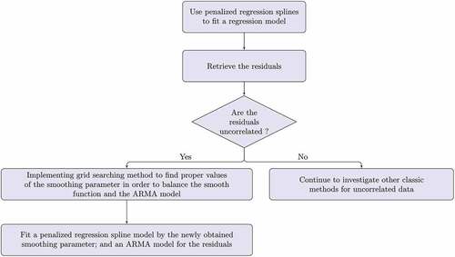
Researchers have developed various techniques to determine suitable values of the smoothing parameter, $\lambda$, for serially correlated data from the perspective of model fitting and statistical inference purpose (e.g., Han & Gu, 2008; A. Liu et al., 2010). While the impacts of the issue on forecasting accuracy are not fully characterised, the confounding of different parts of (3) is a matter of less concern in forecasting, since the primary focus is on improving forecasting accuracy. In case of unsuitable smoothing parameters in the setting of forecasting, we propose a grid search method to select proper smoothing parameters and approach the issue purely from the perspective of forecasting accuracy.

For simplicity of notation, we illustrate the method for a simple version of (3) with

(4) $Y_t=f_1(X_{t1})+f_2(X_{t2})+N_t,$(4)

where $X_{t1}$ and $X_{t2}$ are two univariate variables. Given data $\{(Y_1,X_{11},X_{12}),\dots ,(Y_n,X_{n1},X_{n2})\}$ at time $t=n$, we need to decide proper values for the smoothing parameters denoted by ${\lambda }_1^{\ast }$ and ${\lambda }_2^{\ast }$ to estimate the smooth functions in step $(\mathbf{S}\mathbf{1})$. Based on the cross validation technique (Wood, 2017), a grid search method for proper smoothing parameter, $\lambda$, can be executed as follows:

1. Fit smooth functions ${\hat{f}}_1(X)$ and ${\hat{f}}_2(X)$ to $\{(Y_1,X_{11},X_{12}),\dots ,(Y_n,X_{n1},X_{n2})\}$ for (4) by cross validation and penalised regression and retrieve the smoothing parameters ${\lambda }_1$ and ${\lambda }_2$.

2. Construct the grids of smoothing parameters by ${\upsilon }_1={\lambda }_1\{c_1,\dots ,c_m,1\}$ and ${\upsilon }_2={\lambda }_2\{c_1,\dots ,c_m,1\}$ for which $\{c_1,\dots ,c_m\}$ are $m$ evenly spaced points between some $C_{\mathrm{\ell }}$ and $C_u$ with $0<C_{\mathrm{\ell }}<1$ and $C_u>1$. Let ${\upsilon }_{1j}$ be the $j$ th element of ${\upsilon }_1$ and ${\upsilon }_{2k}$ be the $k$ th element of ${\upsilon }_2$.

3. For each combination of $\{{\upsilon }_{1j},{\upsilon }_{2k}\}$ and a predetermined $s$, examine the performance of $\{{\upsilon }_{1j},{\upsilon }_{2k}\}$ in the past $s$ periods by time $n-1$:

1. For $i=1$ to $s$:

   • Fit a smooth function to $\{(Y_1,X_1),\dots ,(Y_{n-s-1+i},X_{n-s-1+i})\}$ for ((4)) by penalised regression with fixed smoothing parameters $\{{\upsilon }_{1j},{\upsilon }_{2k}\}$ and model the residuals by an ARMA model.

   • Make a forecast for $Y_{n-s+i}$, denoted by ${\hat{Y}}_{n-s+i}$ and compute the squared forecast error $(Y_{n-s+i}-{\hat{Y}}_{n-s+i}{)}^2$.

2. Computer the mean squared errors for the resulting $s$ forecasts.

   1. The final selection of $({\lambda }_1^{\ast },{\lambda }_2^{\ast })$ will be the combination $\{{\upsilon }_{1j},{\upsilon }_{2k}\}$ that induces the minimum mean square errors for the forecasts of the past $s$ periods based on $\{{\upsilon }_{1j},{\upsilon }_{2k}\}$.

For better illustration, the algorithm is called the dynamically balanced spline regression, and its flowchart is provided in Figure 1.

Figure 1. A flowchart for dynamically balanced spline regression.

3. A parallel forecasting strategy of weekly natural gas consumption in the US

Building on the ARMA model and dynamic regression model as well as the dynamic semi-parametric model, we propose a parallel methodology to predict weekly natural gas consumption of the residential and commercial sectors in the US. The proposed model is based on historical natural gas consumption and daily temperature profile to capture the significant effect of weather on natural gas consumption. As shown in Figure 2, the parallel strategy includes three steps:

1. Model the weekly scrape data $Y_t$ and make forecast for ${\hat{Y}}_t$.

2. Model the monthly scale ratio $R_m$ and make forecast for the weekly scale ratio ${\hat{R}}_t$.

3. The forecast for weekly natural gas consumption will be given by ${\hat{Y}}_t\times {\hat{R}}_t$.

Figure 2. A parallel strategy to forecast the weekly natural gas consumption.

First, the pipeline (metre) scrape data refer to the data collected from the operational capacity postings on interstate pipeline Electronic Bulletin Boards as mandated by Order NO. 636 under the capacity release programme of the US Federal Energy Regulatory Commission. The scrape data are available on a daily basis and measured in thousand cubic feet (MSF), million cubic feet (MMcf), or billion cubic feet (BCF). The scrape data from the operational capacity postings represent the total amount of natural gas entering a state through the interstate pipelines and can serve as the major reference for gauging natural gas consumption. It should be noted that since the natural gas brought into a state by the interstate pipelines can continue to be shipped to other states according to the shipment contracts, the particular state of interest sometimes just serves as a transit point, and the total scape data reported by the interstate pipeline companies for a particular state is not equal to the total natural gas consumed by the state. To forecast the true natural gas consumption in the residential and commercial sectors, the scrape data need to be properly scaled (calibrated). Accordingly, we first define the monthly scale ratio, $R_m$, to be

$R_m=\frac{E_m}{Y_m},$

where $Y_m$ denotes the corresponding aggregated monthly scrape data and $E_m$ denotes the EIA published monthly consumption data.

The $E_m$ is monthly natural gas consumption in each state of the US and can be obtained from the EIA, which compiles the energy data from monthly or annual surveys authorised by the US Department of Energy (DOE). The surveys cover a wide range of sources, including the utility industry, energy or conservation agencies in the gas producing states, energy companies that operate underground storage facilities, and companies that deliver natural gas to consumers. The EIA provides the natural gas consumption data of all 51 states, which date back as far as 1973 at monthly or yearly time scales and is useful for scaling the scrape data to reveal the true consumption in each state.

In the forecasting models of the weekly scrape data and the weekly scale ratio, the key predictor variable is Heating Degree Days (HDD), due to the sensitivity of natural gas consumption to weather conditions, particularly temperature. The HDD measures how long (the duration) and how much (the severity) the exterior temperature was below a predetermined reference temperature. The reference temperature is also called the base temperature, with a default value equal to 65 degrees Fahrenheit (${ }^{\circ }F$). The HDD has been used extensively in predicting natural gas consumption (e.g., Brown & Matin, 1995; Gumrah et al., 2001; Herbert, 1987).

Let $(x{)}^{+}=max\{x,0\}$, and the temperature of a day at time $t$ since midnight (in hours) be $T(t)$. The daily HDD can be computed as the total $degree\times hours$ of the day or the 24-hour average of the former value expressed in degrees.

(5) ${\int }_0^{24}{\left(65-T(t)\right)}^{+}dt,or\frac{1}{24}{\int }_0^{24}{\left(65-T(t)\right)}^{+}dt.$(5)

In practice, there exist various approximation methods to calculate the daily HDD values, depending on the available climatic data (De Rosa et al., 2015). If the external temperature hourly profiles, $T_{d,h}$ for $h=1,\dots ,24$, of day $d$ are available, then we can compute its daily HDD as the mean daily $degree\times hours$ via

$\frac{1}{24}\sum _{h=1}^{24}(65-T_{d,h}{)}^{+}.$

Note that the unit for the daily HDD obtained from the above formula is in degrees, since it is obtained as an average value. For other methods of calculating HDD, including the approach proposed by the UK Meteorological Office, please refer to De Rosa et al. (2015). The Integrated Surface Database from the website of National Centers for Environmental Information (NCEI) provides the external hourly summary based on surface observational data, including the external temperature hourly profiles, along with the hourly profiles of many other weather variables, such as dew point, sea level pressure, wind direction, and wind speed.

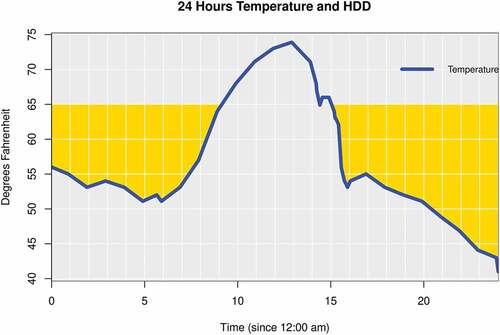
Figure 3 illustrates an example of the 24-hour temperatures recorded on a certain day during the winter time at a weather station in the North Atlantic Region. The total $degree\times hours$ for a base temperature of 65 ${ }^{\circ }F$, denoted by the shaded part between the $65$${ }^{\circ }F$ horizontal line and the temperature curve, is equal to 224, which was obtained by linear interpolation of the boundary of the shaded area. The HDD in terms of a 24-hour average value of ((5)) for Figure 3 is equal to $9.33$ degrees.

Figure 3. Calculating the HDD based on the hourly temperature data: the total area of the region enclosed by the 65 degrees line and the real temperature is around 224 $degree\times hours$.

In this study, to assess the proposed forecasting model, we obtained the HDD data (i.e., calculated as the daily average HDD in ^°F (degrees Fahrenheit) with the base temperature as 65^°F) from one weather station from each of the six states across the New England area. Population map was used to locate a weather station close to where most people live in each state. A weighted HDD was calculated to reflect the overall heating demand as a single index number. A naïve method calculates the weights for the six weather stations, denoted by $\pi =({\pi }_1,\dots ,{\pi }_6{)}^{\mathrm{T}}$, as the historical averages of each state’s proportion of consumption as compared with the total consumption of the six New England states based on the EIA monthly data. Alternatively, to find a proper weight vector, we also took an approach that has been used to solve an optimisation problem numerically with the weights as optimisation parameters (Chapter 7, Wood, 2017). Hereafter, let $Y_t$ be the weekly total sum of the scrape data of the six states in the New England area, $X_t^{\omega }$ is the weighted HDD induced by $\omega =({\omega }_1,\dots ,{\omega }_t{)}^{\mathrm{T}}$, and $U_t$ is the month of the week expressed as an integer from 1 to 12. We picked the optimiser, denoted as ${\omega }_{\ast }$, that minimised the cross validation score for the penalised regression of the model $Y_t=f_1(X_t^{\omega })+f_2(U_t)+{\epsilon }_t$, where $f_1$ and $f_2$ are smooth functions and ${\epsilon }_t$ is assumed to be uncorrelated random errors. It turned out that the performances of $\pi$ and ${\omega }^{\ast }$ are comparable for various forecasting models investigated. Our preference tilted towards $\pi$ due to its simplicity.

We also explored other weather variables in the hourly profiles from the $6$ weather stations. For example, the Wind Chill Temperature Index (WCT) combines the information of temperature and wind speed and measures the common effect of wind and temperature in loss of heat in human body. We incorporated WCT into the forecasting formula by computing a predictor variable from (5) with temperature replaced by WCT. However, compared with the HDD-based models, no significant improvements were observed for the WCT-based models. Taking into account the computational complexity, WCT was dropped from the choices. The HDD is demonstrated to be the most useful predictor variable. Throughout the remainder of this paper, we will use $X_t$ and $X_m$ to denote the weekly total and monthly total of the weighted HDD by $\pi$.

3.1. Forecasting the weekly scrape data

To forecast the weekly scrape data, we specify two groups of models. Within each group, the models are similar in their forms but differ from one another with regard to whether the serial correlations are addressed in the model and how they are addressed. The first group of models takes a common form given by

(6) $Y_t=f_1(X_t)+f_2(U_t)+{\epsilon }_t.$(6)

Let $M_{11}$ be the fitted model of (6) when ${\epsilon }_t$ is assumed to be uncorrelated. Model diagnostics reveal that model $M_{11}$ is not adequate for the data in that the residuals exhibit significant levels of autocorrelation. Further investigation indicates that the autocorrelation resembles those of the classic ARMA models. Accordingly, we propose a variant of (6), taking the form as a simple version of (3),

(7) $\left(\begin{array}{cc}{Y}_t& =f_1(X_t)+f_2(U_t)+{\epsilon }_t\\ {\epsilon }_t& \sim \mathrm{A}\mathrm{R}\mathrm{M}\mathrm{A}(p,q).\end{array}\right.$(7)

Let $M_{12}$ be the fitted model of (7) by the sequential procedure outlined in Section 2 for which the smoothing parameter is determined by the cross validation method with ${\epsilon }_t$ being treated as uncorrelated. Also, we consider a different strategy for fitting (7). Specifically, $M_{12}^{\ast }$ represents the fitted model for (7) by the proposed sequential procedure, with the smoothing parameter determined through the grid search method discussed in Section 2.

The second group of models apply the multi-scale approach of Nedellec et al. (2014). The method decomposes the scrape data into long-term trend part, medium/short-term part, and random error part in a sequence of steps. The constituting parts are modelled by separate modules, and the forecast for the scrape data comprises the sum of the forecasting results from those three parts. We assume that the weekly total of the scrape data is mainly determined by

(8) $Z_t^{\mathrm{\ell }}+Z_t^m+Z_t^s,$(8)

where $Z_t^{\mathrm{\ell }}$ is the long-term part of the weekly scrape data, corresponding to low-frequency variations such as trends, economic effects, and slow changes in natural gas usages; $Z_t^m$ is the medium-term part, incorporating all the meteorological effects; and $Z_t^s$ represents the short-term part, containing everything that could not be captured by the long-term part or medium-term part. The first multi-scale model is defined by

(9) $M_{21}:Y_t=Z_t^{\mathrm{\ell }}+Z_t^m+{\epsilon }_t,$(9)

where ${\epsilon }_t$ is the uncorrelated random error. In (9), we do not model the short-term effects in (8) explicitly and relegate them into the random error ${\epsilon }_t$. The model (9) is estimated sequentially. First, we fit a semi-parametric model through the penalised regression method to the monthly total of the scrape data $Y_m$ and the weighted HDD, $X_m$, by

$Y_m=f(X_m)+U_m+{\epsilon }_m,$

where $U_m$ is the month of the data as an integer from 1 to 12 and ${\epsilon }_m$ is the random error. The $Z_t^{\mathrm{\ell }}$ is estimated by a kernel regression model fitted to the residuals of the above monthly model and the estimation of $Z_t^{\mathrm{\ell }}$ is given by the estimation of the fitted kernel regression model denoted by ${\hat{Z}}_t^{\mathrm{\ell }}$. Second, we treat the de-trended data $W_t=Y_t-{\hat{Z}}_t^{\mathrm{\ell }}$ as the estimate of $Z_t^m+{\epsilon }_t$ and fit a nonparametric model to the de-trended data, $W_t=f_1(X_t)+f_2(U_t)+{\delta }_t$, where ${\delta }_t$ is assumed to be uncorrelated, and the estimate of $Z_t^m$ is given by ${\hat{Z}}_t^m={\hat{f}}_1(X_t)+{\hat{f}}_2(U_t)$. We use $M_{21}$ to denoted the fitted model (9) for which only the regular cross validation method (see Chapter 4, Wood, 2017) is used to select the smoothing parameter for the nonparametric model of the de-trended data and use $M_{21}^{\ast }$ to denote the fitted model when the grid search method proposed in Section 2 is applied for $W_t$.

The second multi-scale model explicitly addresses the autocorrelation

(10) $\left(\begin{array}{cc}{Y}_t& =Z_t^{\mathrm{\ell }}+Z_t^m+{\epsilon }_t\\ {\epsilon }_t& \sim \mathrm{A}\mathrm{R}\mathrm{M}\mathrm{A}(p,q),\end{array}\right.$(10)

where ${\epsilon }_t$ contains the short-term part of (8) and is assumed to follow an ARMA process. The same estimation procedure of $M_{21}$ is applied to (10) with an additional final step in which an ARMA model is fitted to the residuals of the de-trended data. And, the forecast of $Y_t$ is based on the fitted long-term part, de-trended data, and the ARMA model. We use $M_{22}$ to denote the fitted model for (10) when only cross validation is applied to obtain the smoothing parameter, and as $M_{21}^{\ast }$ above, $M_{22}^{\ast }$ denotes its variant where the possible smoothing parameter issue is considered and the proposed grid search method is applied.

3.2. Forecasting the weekly scale ratio

The monthly scale ratio data, $R_m$, exhibit the typical characteristics of seasonal time series (i.e., values are higher during the winter months and lower in the summer months) and do not show apparent trend and remain stable over time. In addition, because natural gas consumption is highly susceptible to weather impacts on residential and commercial usage, the $R_m$ data also demonstrate short-term autocorrelations. Classic seasonal ARMA models and the exponential smoothing methods all seem suffice for the data. However, one difficulty for forecasting $R_m$ is that there exists a lag time of 3 months between the data publishing time on the EIA website and the real time of consumption, which means that the forecasts by seasonal ARMA models or the exponential smoothing methods always have a lead time of $3$ months. It is known that the forecasts by ARMA models converge to a constant level exponentially fast as the lead time increases (Box et al., 2016), and the forecast accuracy of $R_m$ deteriorates quickly as the lead time of forecast increases. At the same time, the forecast accuracy of $R_m$ by exponential smoothing methods also suffers as the lead time of forecast increases. On the other hand, there exists a high correlation between the scale ratio and the daily average of the weighted HDD of each month, $X_m$. Therefore, we introduce a nonparametric model for $R_m$ with the daily average of the weighted HDD, $X_m^a$, as the predictor variable

(11) $R_m=f(X_m^a)+\epsilon ,$(11)

where $\epsilon$ is assumed to be an uncorrelated random error process. The biggest advantage of (11) is that it bypasses the three-month lag time. Let the fitted model of (11) be denoted by $M_3$. When the forecast for the weekly scale ratio is needed, one can simply plug the forecast of the average weighted HDD of the corresponding week into $M_3$ and obtain ${\hat{R}}_t$, as illustrated in Figure 2.

4. Implementation and performance of proposed forecasting strategy

4.1. Model implementation and diagnosis

In order to assess the performance of the proposed parallel strategy, we deployed the forecasting models on empirical data. Specifically, we obtained daily scrape data for the New England region from January $7$, 2013, through February $4$, 2018, for totally 265 weeks. Correspondingly, the HDD data and the EIA monthly natural gas consumption data of the same time period were collected from NCEI and EIA, respectively. 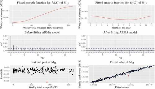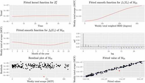The data of the first 212 weeks, from January $7$, 2013, to January $29$, 2017, were used to apply and diagnose the proposed models. Comprehensive diagnostics show that the proposed models for the scrape data are adequate, especially when time series ARMA models are incorporated. In particular, we plot the fitted smooth functions of $M_{12}$ in Figure 4. The fitted smooth curve of HDD effects on natural gas consumption, $f_1(X_t)$, revealed an S-shaped curve that comprises an initial stage with slow growth rates, then a take-off stage with faster growth rates, and a final tapering-off stage with slow growth rates. Figure 4 also indicates that the additive model alone cannot capture the full dynamic of the data, since, after fitting the additive model, the residuals are serially correlated and present the typical ACF of an ARMA model. After fitting a proper ARMA model, the residuals of $M_{12}$ appear uncorrelated. In addition, we plot the residuals of $M_{12}$. It is shown that most of the residuals are evenly distributed around zero, except for the point marked by a star for week $203$, the week from November 21, 2016, to November 27, 2016, for which the fitted value is much greater than the actual value. In the fitted value versus actual value plot, all the points except the point for week 203 are distributed around the line of $y=x$ compactly.

Figure 4. Top left: fitted smooth function of the weekly total weighted HDD for ${\mathrm{M}}_{12}$ for the data from January 7, 2013, to January 29, 2017; Top right: fitted smooth function of month for ${\mathrm{M}}_{12}$; Middle left: the ACF for the residuals of ${\mathrm{M}}_{12}$ before fitting the ARMA model; Middle right: the ACF for the final residuals of ${\mathrm{M}}_{12}$ after fitting the ARMA model; Bottom left: the scatter plot of the final residuals of ${\mathrm{M}}_{12}$; Bottom right: the scatter plot for the weekly total scrape versus the fitted values of ${\mathrm{M}}_{12}$, where the straight line is the 45^° line going through the origin.

In Figure 5, the fitted long-term trend as well as the fitted smooth functions of $f_1(X_t)$ and $f_2(U_t)$ of the de-trended data are plotted. The latter two plots are similar to those of Figure 4. Model $M_{21}$ does not model the serial correlation explicitly. It can be observed that the residuals are weakly correlated. The residual plots resemble those of model $M_{12}$. The fitted smooth functions of $f_1(X_t)$ and $f_2(U_t)$ take values with an order of magnitude equal to $6$, while in contrast, the fitted long-term trend takes values with an order of magnitude of 5. Note that the long-term trend resembles a flattened curve due to the scale of the curve. In fact, if we zoom in the graph or change the scale of the vertical axis to ${10}^5$, we can see a slowly increasing trend of natural gas consumption over time.

Figure 5. Top left: fitted long-term trend of weekly total scrape for ${\mathrm{M}}_{21}$ for the data from January 7, 2013, to January 29, 2017; Top right: fitted smooth function of weekly total weighted HDD for ${\mathrm{M}}_{21}$; Middle left: fitted smooth function of month for ${\mathrm{M}}_{21}$; Middle right: the ACF for the residuals of ${\mathrm{M}}_{21}$; Bottom left: the scatter plot of the final residuals of ${\mathrm{M}}_{21}$; Bottom right: the scatter plot for the weekly total scrape versus the fitted values of ${\mathrm{M}}_{21}$, where the straight line is the 45 ${ }^{\circ }$ line going through the origin.

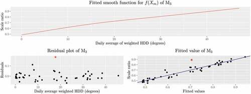
The scale ratio model was fitted to the monthly data. From Figure 6, we can see that the scale ratio and the daily average weighted HDD are positively correlated. The fitted smooth function of $f(X_m)$ demonstrates a slight curvature. The model fits the data very well except for one outlier marked by a star.

Figure 6. Top: fitted $f(X_m)$ of ${\mathrm{M}}_3$; Bottom left: the scatter plot of the residuals of ${\mathrm{M}}_3$ versus the daily average weighted HDD for the data from January 7, 2013, to January 29, 2017; Bottom right: the scatter plot for the scale ratio versus the fitted scale ratio of ${\mathrm{M}}_3$, where the straight line is the 45${ }^{\circ }$ line going through the origin.

4.2. Evaluation of forecasting accuracy

To evaluate the performance of the proposed methodology, we simulated the operations of an energy company by estimating the weekly consumption of natural gas in the residential and commercial sectors of the New England area for 1-year test period from January $30$, 2017, to February $4$, 2018, i.e., week 213 to week 265 in the data set. To mimic the forecasting in a realistic manner, the HDD 7-day forecasts were collected for the regions where the six weather stations of Table 1 are located from the Climate Prediction Center of National Weather Service (NWS). When weekly forecasts need to be made at a specific time point, called the forecasting origin, we assume that the historical scrape data and daily weather data are available up to the date of the forecasting origin, and the EIA historical monthly natural gas consumption data are available up to three months before the forecasting origin. Accordingly, the 7-day HDD forecasts from the NWS for the target week are plugged into the trained models to make forecasts. The evaluation was performed on the basis of a rolling forecasting origin method (Hyndman & Athanasopoulos, 2018) for successively 53 weeks:

1. Starting with week $i=213$, the following procedures are used to obtain the forecast of natural gas consumption for the week $i$..

   1. Use the scrape data and weather data from week $1$ to week $i-1$ to train the models for scrape data;

   2. Use the EIA monthly data, up to 3 months prior to week $i$, to train the model for scale ratio;

   3. Obtain the 7-day HDD forecast for week $i$ and make forecast for ${\hat{Y}}_t$ and ${\hat{R}}_t$;

   4. The forecast of week $i$ is given by ${\hat{V}}_t={\hat{Y}}_t\times {\hat{R}}_t$.

2. Repeat step (a) for $i=214,\dots ,265$.

Table 1. Weather stations and weights for the weighted HDD.

State	Station Code	$\pi$ (%)
MA	KBOS	56.88
CT	KHVN	26.49
RI	KWST	3.82
NH	KMHT	3.18
VT	KVSF	6.82
ME	KPWM	2.81

Prediction accuracy is the most important measure of performance of forecasting methods (Tamba et al., 2018) and the goal of our study. Therefore, to evaluate the performance of the proposed method, we used two forecasting accuracy metrics, i.e., the mean absolute deviation (MAD) and the mean absolute percentage error (MAPE), which are among the most commonly used performance measures in the literature (Tamba et al., 2018). Based on those two metrics, we examined the model’s forecasting accuracy on both weekly and monthly time scales.

For weekly total scrape, MAD is defined by $\mathrm{M}\mathrm{A}\mathrm{D}={\sum }_{t=213}^{265}\left|Y_t-{\hat{Y}}_t\right|/53$, and MAPE is defined by $\mathrm{M}\mathrm{A}\mathrm{P}\mathrm{E}={\sum }_{t=213}^{265}\left|\left(Y_t-{\hat{Y}}_t\right)/Y_t\right|/53$. The MAD and MAPE measures are defined similarly for monthly consumption data. To implement the grid search method proposed in Section 2, the values $C_{\mathrm{\ell }}=0.5$, $C_u=2$, and $s=4$ were used. Table 2 summarises the performance of the proposed models for weekly scrape data $Y_t$. It is evident by comparing the models in $\{{\mathrm{M}}_{11},{\mathrm{M}}_{12}\}$ and the models in $\{{\mathrm{M}}_{21},{\mathrm{M}}_{22}\}$ that the models improved progressively, and incorporating a time series ARMA component into the latter model in each pair increases the forecast accuracy for $Y_t$. Furthermore, the proposed grid search method induced improved accuracy in both MAD and MAPE, which can been observed by comparing the models $\{{\mathrm{M}}_{12},{\mathrm{M}}_{12}^{\ast }\}$, $\{{\mathrm{M}}_{21},{\mathrm{M}}_{21}^{\ast }\}$, and $\{{\mathrm{M}}_{22},{\mathrm{M}}_{22}^{\ast }\}$ in Table 2.

Table 2. Forecast accuracy for weekly total scrape. Running time was recorded on a laptop computer with an Intel Core i7-8550 U CUP @1.80 GHz, by R 4.0.

Model	MAD (MCF)	MAPE	Running Time (sec)
$M_{11}$	772,034.3	0.0773	8.51
$M_{12}$	443,878.6	0.0375	10.87
$M_{12}^{\ast }$	442,252.8	0.0375	1039.32
$M_{21}$	490,675.3	0.0417	10.84
$M_{21}^{\ast }$	444,550.8	0.0377	1055.45
$M_{22}$	473,569.3	0.0404	14.71
$M_{22}^{\ast }$	431,544.1	0.0369	2062.63

Table 3. Forecast accuracy for monthly natural gas consumption in residential and commercial sectors. Running time was recorded on a laptop computer with an Intel Core i7-8550 U CUP @1.80 GHz, by R 4.0.

Model	MAD (MCF)	MAPE	Running Time (sec)
$M_{11}+M_3$	1,699,087	0.0486	10.44
$M_{12}+M_3$	1,252,141	0.0386	12.83
$M_{12}^{\ast }+M_3$	1,239,234	0.0377	1067.15
$M_{21}+M_3$	1,262,696	0.0362	12.24
$M_{21}^{\ast }+M_3$	1,311,587	0.0375	1076.37
$M_{22}+M_3$	1,291,354	0.0374	19.07
$M_{22}^{\ast }+M_3$	1,312,517	0.0376	2095.93

When training scale ratio model, the apparent outlier identified in Figure 6 was deleted. Since the accurate natural gas consumption data of New England area are only available at monthly scales from EIA, the weekly forecasts $\{{\hat{V}}_t{\}}_{t=213}^{265}$ were first aggregated into monthly forecasts and then the forecast accuracy was assessed on a monthly basis. The MAD and MAPE of the proposed strategy for the monthly natural gas consumption data are presented in Table 3. All proposed models performed comparably well, except for $M_{11}+M_3$. In terms of MAD, the combination $M_{12}^{\ast }+M_3$ induced the most accurate result, while in terms of MAPE, the combination $M_{21}+M_3$ performed the best.

4.3. Benchmarking results

Forecasting techniques have been one of the most active research areas in many fields. It is no exception for natural gas consumption forecasting that many methods have been proposed to tackle the problem from various angles with specific targets (see, e.g., Chen et al., 2016; Fan et al., 2013; Olgun et al., 2012; Ozdemir et al., 2016; Karadede et al., 2017; Li et al., 2021, among others). Nevertheless, like previous studies on natural gas consumption forecasting, in this study, the problem of weekly consumption forecasting shares the following three properties..

1. The feature space is enlarged to represent the exquisite relationships between the target variable and predictors by either the kernel method, or the polynomial method, or the spline method.

2. The forecasting is derived through a sequence of steps each of which employs a different inference method to take care of one major constituent component of the target variable.

3. Some hyper-parameters are involved and need to be carefully tuned in order to obtain the best results.

In recent years, deep learning is a boiling hot area in the machine learning and artificial intelligence communities. Due to increasingly powerful computation platforms and new architectures, deep learning achieves a series of successes in dealing with high-dimensional data problems, such as computer vision, machine perception, and natural language understanding. The corner stone of deep learning is artificial neural networks (James et al., 2021). Various artificial neural networks-based methods have been applied to forecast the consumption of natural gas and other fuel types (Soldo, 2012; Tamba et al., 2018). In this study, we thus selected deep learning techniques for benchmarking to assess the performance of the proposed model against other forecasting methods.

First of all, we pilot Deep Neural Network (DNN) method on weekly scrape data forecasting. A DNN represents a neural network with a deep series of fully connected networks. Figure 7 shows the structure of a fully connected neural network with two hidden layers. In practice, a DNN can contain tens of millions of parameters. The DNN is applied with two predictor variables, weekly HDD and month of the year, which are intended to capture the main weather effects and seasonality, respectively. The training of a DNN is a complicated work. Major hyper-parameters include the mini batch size, learning rates, the number of layers, and the number of nodes in each layer. Since DNN is prone to overfitting, regularisation measures were developed to tame the overfitting tendency. Conventional regularisation measures include node dropout and weight regularisation. The dropout rates are treated as a tunable hyper-parameter. We experimented with various settings for the hyper-parameters both manually and autocratically by the auto-tuner. The best DNN delivers forecasting results with MAPE equal to 0.0748 and MAD equal to 777,795.4 MCF, which is comparable with the baseline model $M_{11}$ as reported in Table 2.

Figure 7. A fully connected neural network with two hidden layers.

Next, we investigated a class of prominent deep learning architectures in natural language processing, the so-called Recurrent Neural Network (RNN). This class of architectures possesses the ability of memorising the past information fed into the network and processes sequences of data in chronological order. Figure 8 illustrates the structure of a simple RNN with the RNN cell repeated 10 times. In Figure 8, there are totally 10 time steps involved, and the input sequence is denoted by $\{x_t,\dots ,x_{t-9}\}$. An RNN network iterates through the input sequence chronologically and keeps hidden state variables, denoted by $h_t$ through $h_{t-9}$ in Figure 8, to maintain the sequence information. Additional variants of RNN are derived when delicate mechanisms to carry past information and update state variables are built into the simple RNN. Here two variants of RNN are of interest, long short-term memory (LSTM) neural network and gated recurrent unit (GRU) neural network.

Figure 8. A simple RNN.

In addition to the hyper-parameters associated with DNN, one extra hyper-parameter we need to consider for LSTM or GRU is the number of time steps that the input sequence needs cover. We train the LSTM neural networks and the GRU neural networks both manually and automatically. The top performer, an LSTM neural network, induces a result with MAPE equal to 0.0444 and MAD equal to 520,963.9 MCF. The LSTM and GRU architectures both demonstrate abilities to address the main weather effect, seasonality, and the time series autocorrelation simultaneously. However, an ensuing study of the residuals shows that it cannot satisfactorily take care of the autocorrelations, since the residuals are still significantly serially correlated. Nevertheless, because these two RNN techniques are capable to make inference for correlated data, they perform better than the baseline model $M_{11}$, which does not consider time series serial correlation issue. However, they are not on a par with the best models achieved by our proposed method as shown in Table 2.

A possible improvement for LSTM or GRU is to add an ARMA model to address the serial correlation. But according to our repeated experiments, an LSTM and an ARMA combination or a GRU and an ARMA combination does not improve forecasting accuracy. One explanation for such results is that the resulted combination of LSTM and ARMA or GRU and ARMA overfit the data. Additionally, we investigate the architecture having a 1D convolutional layer overlaid upon a GRU layer. The best neural network with such structure gives an MAPE equal to 0.0588 and an MAD equal to 778,904.1 MCF for weekly scrape data forecast, which is inferior to the best models of the proposed method in this study.

5. Conclusion

Faced with the dynamic natural gas market nowadays, short-term forecasting of natural gas consumption is challenging (Potočnik & Govekar, 2010). For energy companies, obtaining accurate prediction of natural gas consumption in an efficient manner is particularly critical to help firms avoid regulatory penalty, reduce financial loss, and improve operational efficiency. In this study, we propose a parallel forecasting strategy to make weekly natural gas consumption in the US residential and commercial sectors. The proposed method focuses on developing an efficient approach that can deliver accurate forecast of natural gas consumption but without overburdening requirements for data access and collection. The proposed method only requires moderate data inputs, namely the HDD, scrape data, and consumption-based ratio data, which are all readily available on the websites of government agencies such as NCEI or EIA. As short-term natural gas consumption in the US is especially sensitive to weather conditions, the proposed method models temperature-based variables as the primary predictor for natural gas consumption. Both semi-parametric and nonparametric models are incorporated to improve forecast accuracy. Compared with existing methods for natural gas consumption forecasting, the methodology proposed in this paper features the use of penalised regression splines and time series models. The balance between the penalised regression model and the time series model is emphasised, which is missing in the existing literature. We develop an algorithm-based solution to strike a balance for the two competing parts. The empirical example supports the effectiveness of the proposed method. The diagnosis and evaluation of the models using empirical data show that the proposed method delivers considerably accurate predictions as indicated by the low MAPE in Tables 2 and 3. This parallel forecasting strategy is a practical approach that energy companies can use to better forecast residential and commercial natural gas consumption for more effective production, supply, and distribution planning. The proposed method in this study is readily to be extended to other domains with similar forecasting needs, such as those involving estimating the effect of a main predictor variable and addressing the serial correlations in time series. Also, the benchmarking results suggest that it is interesting to explore potential approaches to embed deep learning techniques into a sequence of steps or stages in forecasting processes to develop a refined method to improve forecasting accuracy. But such a combination of methods can be problem specific. Future research is desired to harness the power of deep learning methods in different settings.

Acknowledgement

The authors would like to thank the Associate Editor and two anonymous reviewers for their important and insightful comments that helped to improve the paper. Xiaoyin Wang and Yunwei Cui acknowledge that their work was partially supported by a grant funded by Exelon Generation Company, LLC. (Grant 5040224).

Disclosure statement

No potential conflict of interest was reported by the author(s).

References

- Al-Fattah, S. (2005). Time series modeling for U.S. Natural gas forecasting. Paper presented at the International Petroleum Technology Conference Doha, Qatar. https://doi.org/10.2523/IPTC-10592-MS
- Aras, H., & Aras, N. (2004). Forecasting residential natural gas demand. Energy Sources, 26(5), 463–472. https://doi.org/10.1080/00908310490429740
- Azadeh, A., Asadzadeh, S. M., & Ghanbari, A. (2010). An adaptive network-based fuzzy inference system for short-term natural gas demand estimation: Uncertain and complex environments. Energy Policy, 38(3), 1529–1536. https://doi.org/10.1016/j.enpol.2009.11.036
- Box, G. E., Jenkins, G. M., Reinsel, G. C., & Ljung, G. M. (2016). Time series analysis: Forecasting and control (5th ed.). John Wiley and Sons Inc.
- Brown, R. H., & Matin, I. (1995). Development of artificial neural network models to predict daily gas consumption. Proceedings of IECON ‘95 - 21st Annual Conference on IEEE Industrial Electronics. Orlando, FL, USA. 2, 1389–1394. https://doi.org/10.1109/IECON.1995.484153
- Charlton, N., & Singleton, C. (2014). A refined parametric model for short term load forecasting. International Journal of Forecasting, 30(2), 364–368. https://doi.org/10.1016/j.ijforecast.2013.07.003
- Chen, Y. H., Hong, W. C., Shen, W., & Huang, N. (2016). Electric load forecasting based on a least squares support vector machine with fuzzy time series and global harmony search algorithm. Energies, 9(2), 70. https://doi.org/10.3390/en9020070
- Darbellay, G. A., & Slama, M. (2000). Forecasting the short-term demand for electricity. Do neural networks stand a better chance? International Journal of Forecasting, 16(1), 71–83. https://doi.org/10.1016/S0169-2070(99)00045-X
- De Rosa, M., Bianco, V., Scarpa, F., & Tagliafico, L. A. (2015). Historical trends and current state of heating and cooling degree days in Italy. Energy Conversion and Management, 90, 323–335. https://doi.org/10.1016/j.enconman.2014.11.022
- Dominici, F., McDermott, A., & Hastie, T. J. (2004). Improved semiparametric time series models of air pollution and mortality. Journal of the American Statistical Association, 99(468), 938–948. https://doi.org/10.1198/016214504000000656
- Ediger, V. S., & Akar, S. (2007). ARIMA forecasting of primary energy demand by fuel in Turkey. Energy Policy, 35(3), 1701–1708. https://doi.org/10.1016/j.enpol.2006.05.009
- Fan, G.F., Qing, S., Wang, H., Hong, W.C., & Li, H.J. (2013). Support Vector Regression Model Based on Empirical Mode Decomposition and Auto Regression for Electric Load Forecasting. Energies, 6, 1887–1901. h t t ps://d o i:1 0.3390/en6041887
- Fan, J., & Yao, Q. (2003). Nonlinear time series: Nonparametric and parametric methods. Springer-Verlag.
- Gelo, T. (2006). Econometric modelling of gas demand. Ekonomski Pregled, 57(1–2), 80–96. https://hrcak.srce.hr/clanak/12206
- Gumrah, F., Katircioglu, D., Aykan, Y., Okumus, S., & Kilincer, N. (2001). Modeling of gas demand using degree day concept: Case study of Ankara. Energy Sources, 23(2), 101–114. https://doi.org/10.1080/00908310151092254
- Gutierrez, R., Nafidi, A., & Sanchez, R. G. (2005). Forecasting total natural-gas consumption in Spain by using the stochastic Gompertz innovation diffusion model. Applied Energy, 80(2), 115–124. https://doi.org/10.1016/j.apenergy.2004.03.012
- Han, C., & Gu, C. (2008). Optimal smoothing with correlated data. Sankhya: The Indian Journal of Statistics, 70(1), 38–72. http://www.jstor.org/stable/41234401
- Herbert, J. H. (1987). An analysis of monthly sales of natural gas to residential customers in the United States. Energy Systems and Policy, 10(2), 127–147. https://www.osti.gov/biblio/6667642
- Herbert, J. H., Sitzer, S., & Eades-Pryor, Y. (1987). A statistical evaluation of aggregate monthly industrial demand for natural gas in the USA. Energy, 12(12), 1233–1238. https://doi.org/10.1016/0360-5442(87)90030-2
- Huntington, H. G. (2007). Industrial natural gas consumption in the United States: An empirical model for evaluating future trends. Energy Economics, 29(4), 743–759. https://doi.org/10.1016/j.eneco.2006.12.005
- Hyndman, R. J., & Athanasopoulos, G. (2018). Forecasting: Principles and practice (2nd ed.). OTexts.
- James, G., Witten, D., Hastie, T., & Tibshirani, R. (2021). An introduction to statistical learning: With applications in R. Springer.
- Karadede, Y., Ozdemir, G., & Aydemir, E. (2017). Breeder hybrid algorithm approach for natural gas demand forecasting model. Energy, 141, 1269–1284. https://doi.org/10.1016/j.energy.2017.09.130
- Kaynar, O., Yilmiz, I., & Demirkoparan, F. (2011). Forecasting natural gas consumption with neural network and neuro fuzzy system. Energy Education Science and Technology. Part A: Energy Science and Research, 26(2), 221–238.
- Kizilaslan, R., & Karlik, B. (2008). Comparison neural networks models for short term forecasting of natural gas consumption in Istanbul. Proceedings of applications of digital information and web technologies Ostrava, Czech Republic. ICADIWT, 448–453.
- Laib, O., Khadir, M., & Mihaylova, L. (2018). A Gaussian process regression for natural gas consumption prediction based on time series data Electronics, 2, 1389–1394.21stInternational Conference on Information Fusion (FUSION). UK: Cambridge. https://doi.org/10.23919/ICIF.2018.8455447
- Li, M. W., Wang, Y. T., Geng, J. H., & Hong, W. C. (2021). Chaos cloud quantum bat hybrid optimization algorithm. Nonlinear Dynamics, 103(1), 1167–1193. https://doi.org/10.1007/s11071-020-06111-6
- Liu, H., Liu, D., Zheng, G., & Liang, Y. (2004). Research on natural gas short-term load forecasting based on support vector regression. Chinese Journal of Chemical Engineering, 12(5), 732–736.
- Liu, A., Qin, L., & Staudenmayer, J. (2010). M-type smoothing spline ANOVA for correlated data. Journal of Multivariate Analysis, 101(10), 2282–2296. https://doi.org/10.1016/j.jmva.2010.06.001
- Logan, J., Lopez, A., Mai, T., Davidson, C., Bazilian, M., & Arent, D. (2013). Natural gas in the U.S power sector. Energy Policy, 40(November), 183–195. https://doi.org/10.1016/j.eneco.2013.06.008
- Mac Kinnon, M., Brouwer, J., & Scott, S. (2018). The role of natural gas and its infrastructure in mitigating greenhouse gas emissions, improving regional air quality, and renewable resource integration. Progress in Energy and Combustion Science, 64(January), 62–92. https://doi.org/10.1016/j.pecs.2017.10.002
- Nedellec, R., Cugliari, J., & Goude, Y. (2014). GEFCom2012: Electric load forecasting and backcasting with semi-parametric models. International Journal of Forecasting, 30(2), 375–381. https://doi.org/10.1016/j.ijforecast.2013.07.004
- Olgun, M. O., Ozdemir, G., & Aydemir, E. (2012). Forecasting of Turkey’s natural gas demand using artificial neural networks and support vector machines. Energy Education Science and Technology Part A: Energy and Research, 30(1), 15–20.
- Ozdemir, G., Aydemir, E., Olgun, M. O., & Mulbay, Z. (2016). Forecasting of Turkey natural gas demand using a hybrid algorithm. Energy Sources, Part B: Economics, Planning, and Policy, 11(4), 295–302. https://doi.org/10.1080/15567249.2011.611580
- Panella, M., Barcellona, F., & D’Ecclessia, R. L. (2012). Forecasting energy commodity prices using neural networks. Advances in Decision Sciences, 2012, 1–26. https://doi.org/10.1115/2012/289810
- Pang, B. (2012). Master’s Theses. The impact of additional weather inputs on gas load forecasting. Marquette University. http://epublications.marquette.edu/theses_open/163
- Piggott, J. L. (1983). Use of Box–Jenkins modeling for the forecasting of daily and weekly gas demand. IEE Colloquium Digest, 4(1).
- Potočnik, P., & Govekar, E. (2010). Practical results of forecasting for the natural gas market. In Natural Gas (pp. 371–392). Sciyo.
- Potočnik, P., Soldo, B., Simunovic, G., Saric, T., Jeromen, A., & Govekar, E. (2014). Comparison of static and adaptive models for short-term residential natural gas forecasting in Croatia. Applied Energy, 129(C), 94–103. https://doi.org/10.1016/j.apenergy.2014.04.102
- Reynolds, D. B., & Kolodziej, M. (2009). North American natural gas supply forecast: The Hubbert method including the effects of institutions. Energies, 2(2), 269–306. https://doi.org/10.3390/en20200269
- Sabo, K., Scitovski, R., Vazler, I., & Zekic-Sušac, M. (2011). Mathematical models of natural gas consumption. Energy Conversion and Management, 52(3), 1721–1727. https://doi.org/10.1016/j.enconman.2010.10.037
- Sailor, D., & Munoz, R. (1997). Sensitivity of electricity and natural gas consumption to climate in the USA-methodology and results for eight states. Energy, 22(10), 987–998. https://doi.org/10.1016/S0360-5442(97)00034-0
- Soldo, B. (2012). Forecasting natural gas consumption. Applied Energy, 92(C), 26–37. https://doi.org/10.1016/j.apenergy.2011.11.003
- Soldo, B., Potocnik, P., Simunovic, G., Saric, T., Govekar, E. (2014). Improving the residential natural gas consumption forecasting models by using solar radiation. Energy and Buildings, 69, 498–506. https://doi.org/10.1016/j.enbuild.2013.11.032
- Suykens, J., Lemmerling, P. H., Favoreel, W., De Moor, B., Crepel, M., & Briol, P. (1996). Modelling the Belgian gas consumption using neural networks. Neural Process Letters, 4(3), 157–166. https://doi.org/10.1007/BF00426024
- Szoplik, J. (2015). Forecasting of natural gas consumption with artificial neural networks. Energy, 85(C), 208–220. https://doi.org/10.1016/j.energy.2015.03.084
- Tamba, J. G., Essiane, S. N., Sapnken, E. F., Koffi, F. D., Nsouandélé, J. L., Soldo, B., & Njomo, D., et al. (2018). Forecasting Natural Gas: A Literature Survey. International Journal of Energy Economics and Policy, 8(3), 216–249. https://www.econjournals.com/index.php/ijeep/article/view/6269
- Taspinar, F., Celebi, N., & Tutkun, N. (2013). Forecasting of daily natural gas consumption on regional basis in Turkey using various computational methods. Energy and Buildings, 56, 23–31. https://doi.org/10.1016/j.enbuild.2012.10.023
- Timmer, R. P., & Lamb, P. J. (2007). Relations between temperature and residential natural gas consumption in the Central and Eastern United States. Journal of Applied Meteorology and Climatology, 46(11), 1993–2013. https://doi.org/10.1175/2007JAMC1552.1
- Valero, A., & Valero, A. (2010). Physical geonomics: Combining the exergy and Hubbert peak analysis for predicting mineral resources depletion. Resources Conservation and Recycles, 54(12), 1074–1083. https://doi.org/10.1016/j.resconrec.2010.02.010
- Viet, N. H., & Mandziuk, J. (2005). Neural and fuzzy neural networks in prediction of natural gas consumption. Neural Parallel Scientific Computation, 13(3–4), 265–286.
- Wadud, Z., Dey, H. S., Kabir, M. A., & Khan, S. I. (2011). Modeling and forecasting natural gas demand in Bangladesh. Energy Policy, 39(11), 7372–7380. https://doi.org/10.1016/j.enpol.2011.08.066
- Wang, J., Feng, L., Zhao, L., & Snowden, S. (2013). China’s natural gas: Resources, production and its impacts. Energy Policy, 55, 690–698. https://doi.org/10.1016/j.enpol.2012.12.034
- Wood, S. N. (2017). Generalized additive models: An introduction with R (2nd ed.). Chapman & Hall/CRC.
- Wood, S. N., Li, Z., Shaddick, G., & Augustin, N. H. (2017). Generalized additive models for Gigadata: Modeling the U.K. Black smoke network daily data. Journal of the American Statistical Association, 112(519), 1199–1210. https://doi.org/10.1080/01621459.2016.1195744
- Xu, G., & Wang, W. (2010). Forecasting China’s natural gas consumption based on a combination model. Journal of Natural Gas Chemistry, 19(5), 493–496. https://doi.org/10.1016/S1003-9953(09)60100-6
- Zhu, L., Li, M. S., Wu, Q. H., & Jiang, L. (2015). Short-term natural gas demand prediction based on support vector regression with false neighbors filtered. Energy, 80, 428–436. https://doi.org/10.1016/j.energy.2014.11.083