Non-linear unit root testing with arctangent trend: Simulation and applications in finance

Abstract

We consider arctangent as the logistic function and compute the asymptotic critical values of the related non-linear unit root test via Monte Carlo simulation. While doing so, we got inspiration from some pioneering articles and use first-order Taylor approximation. We observe that this newly proposed test exhibits higher power than some well-known linear and non-linear tests. We apply our test to some stock indexes and find out that a non-linear arctangent trend can be at stage, rather than a linear unit root process.

Keywords:

• unit root test
• smooth transition
• asymptotic distribution

Public Interest Statement

Mean reversion of financial data is vital for both researchers and practitioners since unpredictable random movements deteriorates forecasting. Mean reversion is often tested via linear framework. However, it is widely explored in the literature that there can be situations where financial data involves a non-linear trend rather than a linear one. This phenomenon is particularly apparent for stock prices. We concentrate on these situations and have developed a new non-linear unit root test statistics together with its asymptotic distribution which exhibits more power compared to some other well-known linear and non-linear unit root tests. In addition to the theoretical contribution, we have evidence that our proposed methodology detects mean reversion for some real stock market data while other tests fail to do so.

1. Introduction

Despite designed to detect unit root in time series with linear trends, augmented Dickey–Fuller (ADF) (1979, 1981) test sometimes detects unit root when the series in question is stationary, but displays a smooth transition. The problems with linear detrending is discussed by Carmichael (1928) and he states that linear detrending is inappropriate in the presence of structural breaks; but would be appropriate for situations where the transition from one regime to another is smooth. He introduces the arctangent representation as an alternative to linear trend. Moreover, as Mills and Patterson (2014) points out, Carmichael’s approach displays insight into the issues affecting the choice of break dates and the nature of adjustment between regimes.

Today we encounter smooth transition functions in a different form, mainly in sigmoid-type adjustment functions, such as the logistic function (see especially Teräsvirta, 1994), which are used for testing unit roots (see for instance, Enders & Granger, 1998; Luukkonen, Saikkonen, & Terasvirta, 1988; Van Dijk, Teräsvirta, & Franses, 2002). The pioneering study of Kapetanios, Shin, & Snell (2003) (KSS) offers a very convenient way of deriving the asymptotic distribution of the null hypothesis in the exponential smooth transition autoregressive (ESTAR) framework by taking first-order Taylor approximation of the transition function.

Some studies related to ESTAR function in recent literature can be summarized as follows. Sollis (2014), took into account possible asymmetric structures. Enders and Jones (2014) constructed a unit root test by the usage of Fourier series in order to approximate smooth breaks. Further generalizations and a recent literature survey are given by Chen and Gan (2018).

In this study, we derive the asymptotic distribution of the null hypothesis of a non-stationary time series when the transition function is arctangent. Next, we show that our test has more power than both the ADF and KSS tests. We also demonstrate the size of our test. Thus, in summary, we propose a plausible new transition function which could be used as an alternative unit root testing in the presence of a non-linear trend.

Rest of the study is as follows: Section 2 states the KSS test and our modification to it. Section 3 is devoted to the presentation of the critical values and the asymptotic distribution of our new test. In Section 4, we present size and power. Section 5 is for applications of these tests to certain stock indices. Finally, Section 5 concludes.

2. KSS test and arctangent smooth transition function

As summarized in Hanck (2012), KSS test considers the unit root null H₀: θ = 0 vs. the non-linear alternative H₁: θ > 0 in the ESTAR framework as:(1) $$\mathrm{\Delta }{y}_t=\beta y_{t-1}+\gamma y_{t-1}\left\{1-exp(-\theta y_{t-1}^2)\right\}+{\epsilon }_t,{\epsilon }_t\sim N(0,{\sigma }^2)\text{i.i.d}.$$(1)

The particular choice of $\left\{1-exp(-\theta y_{t-1}^2)\right\}$ comes from the fact that its first-order Taylor approximation is a polynomial yielding an analytically tractable OLS test regression coefficient under the null hypothesis. Now if $\left\{1-exp(-\theta y_{t-1}^2)\right\}$ is replaced by arctan(θy_t-1), we end up with an alternative test statistics. In this vein, we state two propositions:

Proposition 1: Under the null hypothesis with an arctangent trend, the test statistics can be approximated by:(2) $$s=\frac{{\sum }_{t=1}^T{y}_{t-1}^2{\epsilon }_t}{\sqrt{{\sigma }^2\sum _{t=1}^T{y}_{t-1}^4}}$$(2)

where ${\widehat{\sigma }}^2$ is the least squares estimate of σ²

Proof: Testing the null hypothesis H₀: θ = 0 directly is not feasible, since γ is not identified under the null. Following Luukkonen et al. (1988), one can derive a t-type test statistic. If we compute a first-order Taylor series approximation to the arctangent model around zero from(3) $$arctan\left(x\right)=x-\frac{x^3}{3}+\frac{x^5}{5}-\frac{x^7}{7}+\dots$$(3)

we get the auxiliary relation in Equation (4)(4) $$\mathrm{\Delta }{y}_t=\delta y_{t-1}^2+\text{error}$$(4)

The error term consists of the error term ɛ_t stated in arctangent function replaced version Equation (1) already assumed to be i.i.d. and the error arising from first-order Taylor approximation. Therefore, it is denoted as “error” which corresponds to higher order epsilon terms. Hence, the test statistics becomes $t=\frac{\widehat{\delta }}{\text{std}\text{.err.}(\widehat{\delta })}$.

Proposition 2: Under the null hypothesis of the existence of a unit root, (4) has the asymptotic distribution:

(5) $$s\stackrel{d}{\Rightarrow }\frac{\frac{W{(1)}^3}{3}-{\int }_0^{1}W(r)dr}{\sqrt{{\int }_0^{1}W{(r)}^{4}dr}}$$(5)

Proof: Following the assertions in the derivation of the asymptotic distribution of the null hypothesis of the KSS test, we have:(6) $$s=\frac{{\sum }_{t=1}^T{y}_{t-1}^2{\epsilon }_t}{\sqrt{{\widehat{\sigma }}^2{\sum }_{t=1}^T{y}_{t-1}^4}}\stackrel{d}{\Rightarrow }\frac{{\int }_0^{1}W{(r)}^{2}dW(r)}{\sqrt{{\int }_0^{1}W{(r)}^{4}dr}}$$(6)

As ${\widehat{\sigma }}^2\stackrel{p}{\Rightarrow }{\sigma }^2$ under the null, we only need to derive the asymptotic expressions for $\sum _{t=1}^T{y}_{t-1}^2{\epsilon }_t$ and $\sum _{t=1}^T{y}_{t-1}^4$.

For the first expression:

$$\frac{1}{T}\sum _{t=1}^T{y}_{t-1}^2{\epsilon }_t={\sigma }^2\underset{0}{\overset{1}{\int }}W{(r)}^{2}dW(r)={\sigma }^2\left[\frac{W{(1)}^3}{3}-\underset{0}{\overset{1}{\int }}W(r)dr\right]$$

Since from Ito formula, we have:

$$d\left(\frac{W{(r)}^3}{3}\right)=W{\left(r\right)}^{2}dW\left(r\right)+W\left(r\right)dr$$

The second expression can be computed by following Chan and Wei (1988) as:

$$\frac{1}{T^2}\sum _{t=1}^T{y}_{t-1}^4={\sigma }^4\underset{0}{\overset{1}{\int }}W{(r)}^{4}dr$$

and finally,

$$s\stackrel{d}{\Rightarrow }\frac{{\sigma }^2\left[\frac{W{(1)}^3}{3}-{\int }_0^{1}W(r)dr\right]}{\sqrt{{\sigma }^4{\int }_0^{1}W{(r)}^{4}dr}}=\frac{\frac{W{(1)}^3}{3}-{\int }_0^{1}W(r)dr}{\sqrt{{\int }_0^{1}W{(r)}^{4}dr}}$$

3. Asymptotic critical values

In this section, we compare the arctangent and the KSS tests in terms of the critical values. The critical values of the tests are derived from Monte Carlo simulations with a discretization of a Brownian path into T = 1,000 intervals and producing 10,000 replications and are given in Tables 1 and 2, respectively.

Table 1. Asymptotic critical values of KSS test

Significance (%)	Case 1 (no deterministic term)	Case 2 (with constant)	Case 3 (with constant and trend)
1	−2.81	−3.47	−3.91
5	−2.23	−2.91	−3.38
10	−1.94	−2.63	−3.13

Table 2. Asymptotic critical values of the arctangent test

Significance (%)	Case 1 (no deterministic term)	Case 2 (with constant)	Case 3 (with constant and trend)
1	−2.51	−3.44	−3.94
5	−1.97	−2.87	−3.41
10	−1.61	−2.56	−3.13

Figure 1 portrays the histograms of the distribution of the test statistics under the null hypothesis of the arctangent test.

Figure 1. Histograms of the null hypothesis of arctangent test (from left to right, no deterministic term, with constant, with constant and trend).

In fact, since the exponential and arctangent logistic functions display a similar structure in the [0, 1] interval, it is quite natural to end up with close critical values for KSS and arctangent tests as evident in Tables 1 and 2. However, even a slight difference in the test statistics or critical values might change the test result for a given level of significance, depending on the form of the non-linear trend in the data. We depict them with a figure along with LSTAR function for size and power tests in Section 4.

4. Size and power

In this section, we provide size and power of the arctangent test. For all cases, we took a 5% significance level with 1,000 replications.

4.1. Size of the test

For the size test, we use a DGP which exhibits a clear unit root with constant as:

$$y_t=c+\beta y_{t-1}+{\epsilon }_t$$

where c is a positive real, β = 1 and ${\epsilon }_t\sim N\left(0,1\right)\text{i}.\text{i}.\text{d}.$

The results are portrayed in Table 3.

Table 3. Size of the arctangent test

	Case 2 (with constant)			Case 3 (with constant and trend)
β = 1	Arctan	KSS	DF	Arctan	KSS	DF
T = 50	0.04	0.06	0.05	0.04	0.06	0.03
T = 100	0.04	0.05	0.06	0.05	0.07	0.08
T = 200	0.05	0.05	0.08	0.05	0.06	0.07

4.2. Power of the test

For the power test, we will be comparing the arctangent test with KSS test. Here, c is a positive real and ${\epsilon }_t\sim N\left(0,1\right)\text{i}.\text{i}.\text{d}$. for all cases. When the data is generated via KSS DGP as $\mathrm{\Delta }{y}_t=c+\beta y_{t-1}+\gamma y_{t-1}\left\{1-exp(-\theta y_{t-1}^2)\right\}+{\epsilon }_t$ the arctangent test exhibits less power. On the other hand when the data is generated by $\mathrm{\Delta }{y}_t=c+\beta y_{t-1}+\gamma y_{t-1}\left\{arctan(\theta y_{t-1})\right\}+{\epsilon }_t$, then the power of the KSS test diminishes significantly. So in order to accurately compare the powers of these tests, we utilize the well-known LSTAR smooth transition function and use the DGP as by $\mathrm{\Delta }{y}_t=c+\beta y_{t-1}+\gamma y_{t-1}\left\{1/(1+exp\left(-\theta y_{t-1}\right))\right\}+{\epsilon }_t$. 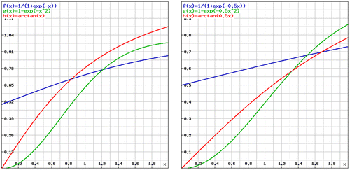Notice that all LSTAR, ESTAR, and arctangent smooth transitions are bounded. These functions are depicted in Figure 2 for different values of $\theta$.

Figure 2. LSTAR, ESTAR, and arctangent logistic functions with θ = 1 (left panel) and with θ = 0.5 (right panel).

In order to have stability β + γ < 0 needs to hold. As we took β = 0.1 (same as KSS test), we vary $\gamma$ parameters from the set $\gamma =\left\{-1.0,-0.5,-0.25,-0.15\right\}$. Moreover, we consider different curvatures $\theta =\left\{0.01,0.05,0.1,1\right\}$. We took different time interval values represented by T as 50,100, and 200 (the reader can consult KSS test for a detailed explanation and choice of parameters). The results show that arctangent test has more power than KSS for almost all cases. Since our DGP is based on a constant term without trend, we expect the powers for Case 2 to be higher than Case 3 which indeed turn out to be the case. When examined further, the more linear the LSTAR function becomes (when θ approaches to 0), the more powerful becomes the DF test compared to arctangent and KSS tests. In addition, the magnitude of $\gamma$ is crucial in the sense that it determines the pullback rate which compensates the impact of $\beta$. Although for lower values of $\gamma$, DF test outperforms the arctangent test, for higher values the opposite is the situation. Nevertheless, arctangent test exhibits higher power than KSS test regardless of the curvature of the LSTAR function. Results are presented in Table 4.

Table 4. Power of the arctangent test

Case 2 (with constant)
	θ = 0.01			θ = 0.05			θ = 0.1			θ = 1
	Arctan	KSS	DF	Arctan	KSS	DF	Arctan	KSS	DF	Arctan	KSS	DF
γ = −1.0
T = 50	0.876	0.749	0.955	0.927	0.829	0.983	0.953	0.869	0.992	0.995	0.991	0.998
T = 100	0.999	0.989	1.000	1.000	0.994	1.000	1.000	1.000	1.000	1.000	1.000	1.000
T = 200	1.000	1.000	1.000	1.000	1.000	1.000	1.000	1.000	1.000	1.000	1.000	1.000
γ = −0.5
T = 50	0.499	0.435	0.549	0.642	0.534	0.661	0.747	0.655	0.743	0.913	0.802	0.961
T = 100	0.894	0.804	0.922	0.969	0.918	0.983	0.993	0.972	0.995	1.000	0.990	1.000
T = 200	1.000	0.993	1.000	1.000	1.000	1.000	1.000	1.000	1.000	1.000	1.000	1.000
γ = −0.25
T = 50	0.340	0.351	0.271	0.553	0.540	0.481	0.652	0.615	0.543	0.486	0.414	0.534
T = 100	0.809	0.793	0.790	0.928	0.894	0.879	0.943	0.894	0.900	0.872	0.762	0.918
T = 200	0.990	0.980	0.986	1.000	0.996	0.996	1.000	0.999	1.000	1.000	0.993	1.000
γ = −0.15
T = 50	0.007	0.011	0.005	0.444	0.454	0.369	0.516	0.536	0.448	0.342	0.329	0.328
T = 100	0.800	0.834	0.639	0.972	0.963	0.939	0.946	0.931	0.931	0.717	0.648	0.709
T = 200	1.000	1.000	1.000	1.000	1.000	1.000	0.999	0.997	0.999	0.950	0.890	0.959

Case 3 (with constant and trend)
	θ = 0.01			θ = 0.05			θ = 0.1			θ = 1
	Arctan	KSS	DF	Arctan	KSS	DF	Arctan	KSS	DF	Arctan	KSS	DF
γ = −1.0
T = 50	0.694	0.517	0.846	0.799	0.644	0.910	0.851	0.720	0.936	0.980	0.970	0.992
T = 100	0.992	0.953	1.000	0.999	0.974	1.000	1.000	0.994	1.000	1.000	1.000	1.000
T = 200	1.000	1.000	1.000	1.000	1.000	1.000	1.000	1.000	1.000	1.000	1.000	1.000
γ = −0.5
T = 50	0.247	0.192	0.240	0.340	0.277	0.331	0.480	0.381	0.455	0.743	0.574	0.826
T = 100	0.666	0.563	0.645	0.841	0.733	0.873	0.950	0.879	0.940	0.999	0.973	0.998
T = 200	0.990	0.961	0.994	1.000	0.996	1.000	1.000	1.000	1.000	1.000	1.000	1.000
γ = −0.25
T = 50	0.066	0.048	0.047	0.143	0.124	0.071	0.225	0.204	0.132	0.239	0.172	0.227
T = 100	0.213	0.178	0.106	0.466	0.446	0.370	0.656	0.590	0.502	0.637	0.485	0.636
T = 200	0.663	0.615	0.547	0.944	0.911	0.920	0.994	0.975	0.978	0.985	0.928	0.991
γ = −0.15
T = 50	0.026	0.028	0.052	0.052	0.049	0.013	0.091	0.064	0.026	0.094	0.061	0.060
T = 100	0.146	0.221	0.010	0.192	0.241	0.072	0.333	0.310	0.165	0.196	0.176	0.148
T = 200	0.291	0.602	0.058	0.865	0.871	0.683	0.892	0.843	0.755	0.573	0.479	0.550

5. Application to financial data

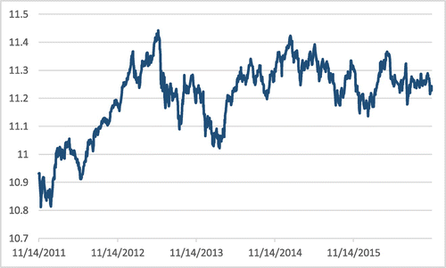
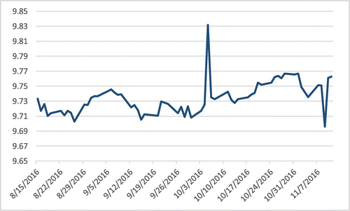
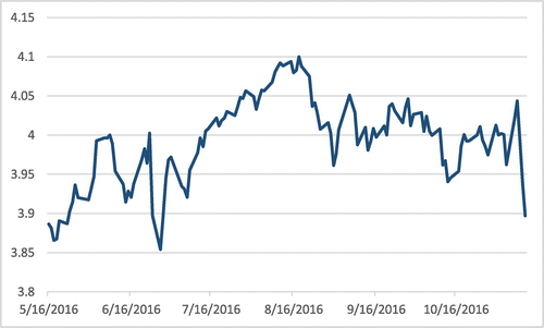
In the empirical analysis, we take time series of three stock indexes namely Turkish BIST 100, Japan Nikkei 225, and South African FTSE/JSE indexes depicted in Figures 3–5.

Figure 3. Logarithm of BIST 100 Index between December 2011 and December 2016.

Figure 4. Logarithm of Nikkei 225 Index between August 2016 and December 2016.

Figure 5. Logarithm of FTSE/JSE Index between May 2016 and December 2016.

For convenience, we take the natural logarithm of the data in question. ADF, KSS, and arctangent unit root test results are given in Tables 5, 6, and 7, respectively.

Table 5. ADF test results

Case 2 (with constant)		Case 3 (with constant and trend)
Index	t-statistics	Index	t-statistics
BIST 100	−2.5556	BIST 100	−2.5591
Nikkei 225	−2.8746*	Nikkei 225	−2.9026
FTSE/JSE	−2.5753*	FTSE/JSE	−2.1980

*Denotes 10% significance level.

**Denotes 5% significance level.

***Denotes 1% significance level.

Table 6. KSS test results

Case 2 (with constant)		Case 3 (with constant and trend)
Index	t-statistics	Index	t-statistics
BIST 100	−2.5800	BIST 100—5 year	−2.5862
Nikkei 225	−2.8785*	Nikkei 225—3 month	−2.9024
FTSE/JSE	−2.5651	FTSE/JSE—6 month	−2.1890

^*Denotes 10% significance level.

**Denotes 5% significance level.

***Denotes 1% significance level.

Table 7. Arctangent test results

Case 2 (with constant)		Case 3 (with constant and trend)
Index	t-statistics	Index	t-statistics
BIST 100—5 year	−2.5678*	BIST 100—5 year	−2.5728
Nikkei 225—3 month	−2.8785**	Nikkei 225—3 month	−2.9025
FTSE/JSE—6 month	−2.5703*	FTSE/JSE—6 month	−2.1936

*Denotes 10% significance level.

**Denotes 5% significance level.

***Denotes 1% significance level.

We clearly see that all tests claim non-stationarity for all the time series for case 3.

However, for Case 2, the ADF and KSS test claims stationarity only for Nikkei 225 index at 10% significance level, whereas arctangent test detects stationarity for all series (BIST 100, 10%, Nikkei 225, 5% and FTSE/JSE, 10%). Notice further that the significance level of the arctangent test is higher than ADF and KSS tests for Nikkei 225 index.

6. Conclusion

It is a widely known fact that certain economic and financial data exhibit smooth transition which ADF test sometimes fails to capture. In that regard, we modify one of the most cited and appreciated non-linear tests namely the KSS test. Having known the arctangent as the precursor of smooth transitions, we replace the logistic function using that particular functional form.

After the computation of critical values and asymptotic distributions, we demonstrate that arctangent test may sometimes reject the presence of unit root where a conventional linear test (ADF) or a non-linear one (KSS) fails to do so. So, we deduce that arctangent test is quite powerful compared to ADF and KSS tests when there is a smooth transition in the data. We applied our findings to three stock indexes for evidence. Researchers can apply this new arctangent test along with ADF and KSS tests in case a smooth transition is suspected in the data, but ADF and KSS tests fail to detect stationarity.

Funding

The author received no direct funding for this research.

Additional information

Notes on contributors

Deniz Ilalan

The authors are interested in stochastic modeling of asset prices and applied econometrics. They both pursue their academic career on financial mathematics. Their collective research is particularly on mean reversion concepts in interest rates and stock prices. They aim to develop other unit root testing methodologies with both theory and empirical applications as future research. Apart from their common studies, Deniz Ilalan concentrates on applications of fractal geometry in finance and Levy processes. On the other hand, Özgür Özel’s research interests include monetary policy, macroeconomy, and forecasting.

References

- Carmichael, F. L. (1928). The arctangent in trend determination. Journal of the American Statistical Association, 23, 253–262.10.1080/01621459.1928.10503020
- Chan, N. H., & Wei, C. Z. (1988). Limiting distributions of least squares estimates of unstable autoregressive processes. Annals of Statistics, 16, 367–401.10.1214/aos/1176350711
- Chen, G., & Gan, M. (2018). Generalized exponential autoregressive models for nonlinear time series: Stationarity, estimation and applications. Information Sciences, 438, 46–57.10.1016/j.ins.2018.01.029
- Dickey, D. A., & Fuller, W. A. (1979). Distribution of the estimators for autoregressive time series with a unit root. Journal of the American Statistical Association, 74, 427–431.
- Dickey, D. A., & Fuller, W. A. (1981). Likelihood ratio statistics for autoregressive time series with a unit root. Econometrica, 49(4), 1057–1072.10.2307/1912517
- Enders, W., & Granger, C. W. J. (1998). Unit root tests and asymmetric adjustment with an example using the term structure of interest rates. Journal of Business and Economics Statistics, 16, 304–311.
- Enders, W., & Jones, P. (2014). Grain prices, oil prices, and multiple smooth breaks in a VAR. Studies in Nonlinear Dynamics and Econometrics, 20(4), 399–419.
- Hanck, C. (2012). On the asymptotic distribution of a unit root test against ESTAR alternatives. Statistics and Probability Letters, 82, 360–364.10.1016/j.spl.2011.11.001
- Kapetanios, G., Shin, Y., & Snell, A. (2003). Testing for a unit root in the nonlinear STAR framework. Journal of Econometrics, 112, 359–379.10.1016/S0304-4076(02)00202-6
- Luukkonen, R., Saikkonen, P., & Terasvirta, T. (1988). Testing linearity against smooth transition autoregressive models. Biometrika, 75, 491–499.10.1093/biomet/75.3.491
- Mills, T. C., & Patterson, K. D. (2014). Modelling the trend: The historical origins of some methods and ideas. Journal of Economic Surveys, 29(3), 527–548.
- Sollis, R. (2014). Asymmetric adjustment and smooth transitions: A combination of some unit root tests. Journal of Time Series Analysis, 25, 409–417.
- Teräsvirta, T. (1994). Specification, estimation, and evaluation of smooth transition autoregressive models. Journal of the American Statistical Association, 89, 208–218.
- Van Dijk, D., Teräsvirta, T., & Franses, P. H. (2002). Smooth transition autoregressive models – A survey of recent developments. Econometric Reviews, 21, 1–47.10.1081/ETC-120008723